Regularizing thermo and magnetic contributions within nonrenormalizable theories

Abstract

The importance of implementing a proper regularization procedure in order to treat thermo and magnetic contributions within nonrenormalizable theories is investigated. Our study suggests that potential divergences should be isolated into the vacuum and purely magnetic contributions and then regularized while the convergent thermomagnetic contributions should be integrated over the full momentum range. This prescription is illustrated by applying the proper time formalism to the two flavor Polyakov–Nambu–Jona-Lasinio model, whose magnetic field dependent coupling has been recently determined. Observables such as the pressure, magnetization, speed of sound squared, and specific heat evaluated within our scheme are compared with results furnished by other three possible prescriptions. We show that these quantities display a thermomagnetic behavior which is physically more consistent when our scheme is adopted. In particular, we demonstrate that naively regulating the (entangled) vacuum, magnetic and thermomagnetic contributions leads to physically inconsistent results especially at the high temperature domain.

I Introduction

Understanding the behavior of magnetized quark matter is of fundamental importance for the correct description of physical situations that may take place in magnetars as well as in peripheral heavy ion collisions [1, 2, 3, 4]. On the theoretical side this problem has received a lot of attention recently through the use lattice QCD (LQCD) numerical simulations and analytical model approximations. One controversy has emerged when precise LQCD applications, carried out at zero baryonic densities and physical pionic masses, have indicated that the crossover pseudocritical temperature ($T_{pc}$) should decrease with increasing magnetic field values [5, 6]. This outcome contradicts early LQCD simulations [7, 8, 9], where high pionic mass values were considered, and also analytical evaluations (mostly at the mean field level) performed with effective theories such as the Nambu–Jona-Lasinio model (NJL) [11, *Nambu:1961fr] and the quark meson model (QMM)[13, 14] as well as their Polyakov loop extended versions (PNJL [15] and PQMM [16] respectively). The possible origin of this discrepancy has later been elucidated in Ref. [17] where the authors have shown that adding pionic loops to the mean field quark pressure could fix the problem. Another possible alternative is to include thermomagnetic effects on the coupling constants [18, 19, 20, 21, 22, 23, 24]. This approach has been adopted in various investigations where different possible ansatz [25, 26, 27, 28] to describe the $B$-dependent running of the coupling have been proposed leading to results for $T_{pc}$ which are in line with LQCD predictions. The same type of technique has been generalized to the SU(3) PNJL model where the six fermion coupling has also been fixed according to LQCD data [29]. The reader is referred to Ref. [30] for a comprehensive review on effective models under strong magnetic fields.

Recently, the two-flavor PNJL model coupling has been fixed by using, as input, LQCD results that determine the baryon spectrum of 1+1+1-flavors in the presence of a strong magnetic background and at physical pionic masses [26]. In this case, the running coupling, $G(B)$, has been determined by constraining the PNJL constituent quark mass to match the LQCD results including, of course, the decrease of $T_{pc}$ with $B$. For the present work, it is important to remark that to evaluate quantities such as the pressure the authors of Ref. [26] have adopted Schwinger’s proper time formalism [31] and regularized all integrals without separating the divergent (vacuum) piece from the convergent (thermomagnetic) contribution. Next, this regularization choice has been used to evaluate the effective mass, the quark condensate, and the pressure for $eB=0$ to $0.6\;{\rm GeV}^{2}$ covering temperatures up to $T\approx 0.27\;{\rm GeV}$ so that the final result for $T_{pc}(B)$ is in good agreement with LQCD predictions. Nevertheless, it is now well established that such a regularization procedure can give rise to a series of inconsistencies if the calculations are pushed to higher temperatures (when, e.g., the pressure may not converge to the Stefan-Boltzmann limit, as observed in the case $eB=0$ [32, 33, 34]) or to finite baryon chemical potentials (where the appearance of unphysical oscillations is more noticeable). For example, using a $B$-dependent regularization scheme for the calculation of the magnetization, some authors find oscillations which are unphysical while others find imaginary meson masses which are in fact spurious solutions due to the inappropriate choice of the regularization. This can be seen by comparing the meson masses results of Ref. [35] where real values can only be reproduced upon implementing a consistent regularization strategy.

The importance of using an appropriate regularization scheme to describe magnetized quark matter has been clearly demonstrated in Refs. [36, 37, 38] which suggest a strong dependence on the choice of the regularization scheme for the calculation of physical observables and, more importantly, that an inappropriate regularization scheme may give rise to spurious solutions. Here, our main goal is to investigate different regularization schemes in order to select the ones which produce physically more reliable results as far as nonrenormalizable theories are concerned. With this aim it is important to first recall the possibility that different regularization (and renormalization) procedures implemented to treat divergences in quantum field theories always introduce some degree of arbitrariness during formal evaluations. Generally, within renormalizable theories such as QCD this arbitrariness is associated to the possibility of choosing different regulators, subtraction points, and energy scales. However, physically unambiguous results may be obtained by further constraints such as the ones imposed by the renormalization group equations which require that physical observables be invariant with respect to changes in the arbitrary energy scale. The situation is less clear when it comes to nonrenormalizable theories such as the PNJL model in $3+1d$ considered here. Traditionally, this type of theory is regularized with a sharp cutoff , $\Lambda$, which instead of being removed by some subtraction prescription is formally treated as a “parameter” that sets the energy scale value (generally $\sim 0.6-1\,{\rm GeV}$) up to which the theory can be considered to be effective [40]. In the absence of control parameters such as $T$, $\mu$, and $B$, where it is free from ambiguities, this became the standard procedure to deal with NJL type of models. The case of $T=B=0$ and $\mu\neq 0$ is also unambiguous since the Fermi momentum, $p_{F}=(\mu^{2}-M^{2})^{1/2}$, naturally regularizes the convergent contributions. When finite temperatures come into play (still at $B=0$), the thermodynamical potential at the (one loop) mean field level considered here splits into two parts, $\Omega=\Omega_{V}+\Omega_{T}$. The first represents the ultraviolet (UV) divergent vacuum piece and the second one represents the convergent thermal contribution. In renormalizable theories, one usually isolates and renormalizes the divergences contained in $\Omega_{V}$ so that its final contribution is finite in the extreme UV limit and does not depend on any regulator. At the same time, the convergent thermal integrals are simply integrated over the full momentum range. When considering nonrenormalizable theories where the final vacuum contribution depends on the regulator (now a finite valued parameter), one has two options to treat the thermal part. In early works (see Ref. [41] and references therein), the preferred method was that (for “consistency”) one should also regularize the convergent thermal integrals so that $\Omega=\Omega_{V}(\Lambda)+\Omega_{T}(\Lambda)$. Later, it has been suggested that this course of action is unnecessary since the finite temperature contribution has a natural cutoff in itself specified by the temperature [42] and in this case one should consider $\Omega=\Omega_{V}(\Lambda)+\Omega_{T}(\infty)$. The drawback associated with the former approach is that thermodynamical quantities evaluated in this way do not converge to the expected Stefan-Boltzmann limit as $T\to\infty$ [41]. On the other hand, although the latter strategy does not spoil the high-$T$ behavior of quantities such as the pressure, it can generate thermal effective masses which are smaller than the actual current mass value, $m_{c}$. Although happening at temperatures of the order $T\approx M(0)\approx 300\;{\rm MeV}$, this is still an undesirable feature [34]. It should be mentioned that alternatives to recover the Stefan-Boltzmann limit while maintaining $M(T)>m_{c}$ at high-$T$ have been given in Refs. [43, 44].

Additional care is needed when regularizing a nonrenormalizable theory to describe magnetized hadronic matter due to the Landau level (LL) structure acquired by the vacuum energy. To treat this situation, a seminal work [45] employed the proper time formalism without disentangling the purely magnetic part from the vacuum so that $\Omega=\Omega_{VM}(\Lambda)$. Adding finite temperature effects brings in, once again, the question about the need to regularize (or not) the finite thermomagnetic contribution, $\Omega_{TM}$. Since these two possibilities will be examined here, let us dub standard proper time (SPT) the one in which this term is not regularized so that $\Omega=\Omega_{VM}(\Lambda)+\Omega_{TM}(\infty)$. At the same time, let us dub thermomagnetic regulated proper time scheme (TRPT), the one in which $\Omega_{TM}$ is regularized as in Ref. [26] so that $\Omega=\Omega_{VM}(\Lambda)+\Omega_{TM}(\Lambda)$. Later, the interesting possibility of isolating all the divergences within the vacuum term by separating a finite purely magnetic term (summed over all LL) has been suggested [46, 47]. This scheme, which avoids unphysical oscillations, was originally applied in the proper time (PT) framework [47] and latter generalized to the sharp cutoff framework [48] allowing for several further applications [49, 50, 51, 52, 53, 54, 38, 37, 55]. Within this magnetic field independent regularization scheme (MFIR), which uses dimensional regularization techniques, a magnetic field dependent divergence is subtracted together with other finite mass independent ($B$-dependent) terms so that, at $T=0$, one ends up with $\Omega=\Omega_{V}(\Lambda)+\Omega_{M}$ where $\Omega_{M}$ represents a purely magnetic finite contribution that does not require further integration or sum over LL. As before, when going to finite temperatures, one needs to add the thermomagnetic contribution $\Omega_{TM}(\Lambda)$ or $\Omega_{TM}(\infty)$ to $\Omega$ (here we will consider the latter case which is the one most adopted in the literature).

At this point, it is legitimate to ask how the MFIR subtraction prescription may affect physical observables since subtracting mass-independent terms means that finite $B$-dependent terms also end up by being neglected. Adopting this scheme to analyze phase transitions as in Refs. [46, 48] through order parameters such as the quark condensate, $\langle{\overline{\psi}}\psi\rangle=\partial\Omega/\partial m_{c}$, can be justified by the fact that these quantities are mass dependent. However, the same scheme is certainly not appropriate to treat quantities such as the magnetization, ${\cal M}=-\partial\Omega/\partial B$. This is because a flawless evaluation of $\cal M$ requires the knowledge of the complete $\Omega$ including all finite $B$-dependent terms (see Ref. [56] for a related discussion). In order to circumvent this eventual problem, a fourth possibility which avoids any subtractions will be proposed in the present work. Within this prescription one starts by isolating the purely magnetic part of $\Omega$ and then identifying two potential divergences: one that is $B$-independent ($M$-dependent) and another one which is $B$-dependent ($M$-independent) just as in the MFIR case. However, the most important difference is that now the $B$-dependent divergence is simply regularized but not subtracted (by renormalizing $B^{2}$) as in the MFIR case. Therefore, at $T=0$, the thermodynamical potential has the form $\Omega=\Omega_{V}(\Lambda)+\Omega_{M}(\Lambda)$ [when considering the $T\neq 0$ case in this scheme we will consider a nonregularized piece, $\Omega_{TM}(\infty)$]. We shall dub this prescription vacuum magnetic regularization (VMR) scheme since the divergences present in the vacuum and purely magnetic contributions are regulated. In summary, the fact that at $B\neq 0$ the Lagrangian density of nonrenormalizable models is enlarged by a finite QED type of sector together with the additional possible choices of regularizing the convergent thermomagnetic part generates a great number of possible regularization prescriptions. Unfortunately, dealing with divergences in nonrenormalizable theories in the presence of a magnetic field and a thermal bath cannot be dealt with in a pragmatic manner as in the case of renormalizable theories where further constraints based on a well-established renormalization programme are available. Nevertheless, one may select the most effective one by analyzing the physical behavior of different observables. With this purpose in this work, we will consider the four possible regularization schemes already described to evaluate physical quantities such as the quark condensate, pressure, magnetization, speed of sound, and specific heat at finite temperatures and in the presence of a strong magnetic field. The work is organized as follows. In the next section, we present the model and review finite temperature results in the absence of magnetic fields. Then, in Sec.III, we obtain the thermodynamical potential using four possible regularization prescriptions. Numerical results are presented in Sec. IV and the conclusions in Sec. V.

II The model

The PNJL Lagrangian density in the presence of an external magnetic field is given by [42]

$$\mathcal{L}_{PNJL}=\bar{\psi}\left(i\gamma_{\mu}D^{\mu}-\hat{m}_{c}\right)\psi+G\left[\left(\bar{\psi}\psi\right)^{2}+\left(\bar{\psi}i\gamma_{5}\boldsymbol{\tau}\psi\right)^{2}\right]-\mathcal{U}\left(\Phi,\bar{\Phi},T\right)-\dfrac{1}{4}F^{\mu\nu}F_{\mu\nu},$$ (1)

where $\psi$ represents fermionic fields (a sum in color and flavor indices is implicit), $\tau$ are isospin Pauli matrices, $\hat{m}_{c}$ are the current quark masses which, for simplicity, we set as $m_{u}=m_{d}\equiv m_{c}$ while $G$ represents the coupling constant. The covariant derivative is given by

$$D^{\mu}=\partial^{\mu}-iq_{f}A_{EM}^{\mu}-iA^{\mu}\;,$$ (2)

where $q_{f}$ represents the quark electric charge, $A_{EM}^{\mu}$ is the electromagnetic gauge field, $F^{\mu\nu}=\partial^{\mu}A_{EM}^{\mu}-\partial^{\nu}A_{EM}^{\nu}$ where $A_{EM}^{\mu}=\delta_{\mu 2}x_{1}B$ and $\vec{B}=B\hat{e}_{3}$ within the Landau gauge adopted here. We also consider the Polyakov gauge where the gluonic term, $A^{\mu}=gA^{\mu}_{a}\left(x\right)\frac{\lambda_{a}}{2}$, only contributes with the spatial components: $A^{\mu}=\delta^{0}_{\mu}A^{0}=-i\delta^{0}_{\mu}A^{4}$ where $g$ is the strong coupling, $A^{\mu}_{a}\left(x\right)$ represents the SU(3) gauge fields while $\lambda_{a}$ are the Gell-Mann matrices.  The expectation value of the Polyakov loop, $\Phi$, is then given by the expected value of the Wilson line [57], $L\left(\boldsymbol{x}\right)\equiv\mathcal{P}\exp\left[i\int^{\beta}_{0}d\tau A_{4}\left(\tau,\boldsymbol{x}\right)\right]$. That is,

$$\Phi\equiv\left<\dfrac{1}{N_{c}}\text{Tr}L\left(\boldsymbol{x}\right)\right>,\ \ \ \text{and}\ \ \ \bar{\Phi}\equiv\left<\dfrac{1}{N_{c}}\text{Tr}L^{\dagger}\left(\boldsymbol{x}\right)\right>.$$ (3)

Remark that the Polyakov potential, $\mathcal{U}\left(\Phi,\bar{\Phi},T\right)$, is fixed to reproduce pure-gauge LQCD results [15]. In the case of vanishing baryonic densities ($\mu=0$) considered here, one has $\bar{\Phi}=\Phi$ so that the ansatz proposed in Ref. [58] reads

$$\dfrac{\mathcal{U}\left(\Phi,T\right)}{T^{4}}=-\dfrac{1}{2}b_{2}\left(T\right)\Phi^{2}+b_{4}\left(T\right)\ln\left[1-6\Phi^{2}+8\Phi^{3}-3\Phi^{4}\right],$$ (4)

with

$$b_{2}\left(T\right)=a_{0}+a_{1}\left(\dfrac{T_{0}}{T}\right)+a_{2}\left(\dfrac{T_{0}}{T}\right)^{2},\ \ b_{4}\left(T\right)=b_{4}\left(\dfrac{T_{0}}{T}\right)^{3},$$ (5)

where the parametrization is given in Table 1. Following Ref. [26], we choose $T_{0}=208$ MeV in order to consider two quark flavor contributions [59].

$a_{0}$	$a_{1}$	$a_{2}$	$b_{4}$
3.51	-2.47	15.22	-1.75

Table 1: Parameter set used for the Polyakov loop potential.

III Thermodynamical potential evaluations

Let us now evaluate the thermodynamical potential, $\Omega\left(M,\Phi,T,B\right)$, by applying the MFA to the PNJL within the PT framework. As discussed in the Introduction, the divergences will be handled in four different ways.

III.1 TRPT and SPT frameworks

Within the regulated thermomagnetic integral PT formalism (TRPT) adopted in Ref. [26], the thermodynamical potential is

$$\Omega_{TRPT}(M,\Phi,T,B)=\mathcal{U}\left(\Phi,T\right)+\frac{(M-m_{c})^{2}}{4G}+\frac{N_{c}}{8\pi^{2}}\sum_{f=u,d}(|q_{f}|B)^{2}\int_{\frac{|q_{f}|B}{\Lambda^{2}}}^{\infty}\frac{ds}{s^{2}}e^{-\frac{M^{2}s}{|q_{f}|B}}\coth(s)$$

$$+\frac{1}{8\pi^{2}}\sum_{f=u,d}(|q_{f}|B)^{2}\int_{\frac{|q_{f}|B}{\Lambda^{2}}}^{\infty}\frac{ds}{s^{2}}e^{-\frac{M^{2}s}{|q_{f}|B}}\coth(s)\left\{2\sum_{n=1}^{\infty}e^{-\frac{|q_{f}|Bn^{2}}{4sT^{2}}}(-1)^{n}\left[2\cos\left(n\cos^{-1}\frac{3\Phi-1}{2}\right)+1\right]\right\}\;,$$ (6)

where the effective mass is given by the solution of the self-consistent gap equation

$$\frac{M-m_{c}}{2G}=\frac{MN_{c}}{4\pi^{2}}\sum_{f=u,d}|q_{f}|B\int_{\frac{|q_{f}|B}{\Lambda^{2}}}^{\infty}\frac{ds}{s}e^{-\frac{M^{2}s}{|q_{f}|B}}\coth(s)$$

$$+\frac{M}{4\pi^{2}}\sum_{f=u,d}|q_{f}|B\int_{\frac{|q_{f}|B}{\Lambda^{2}}}^{\infty}\frac{ds}{s}e^{-\frac{M^{2}s}{|q_{f}|B}}\coth(s)\left\{2\sum_{n=1}^{\infty}e^{-\frac{|q_{f}|Bn^{2}}{4sT^{2}}}(-1)^{n}\left[2\cos\left(n\cos^{-1}\frac{3\Phi-1}{2}\right)+1\right]\right\}\;,$$ (7)

which is to be solved simultaneously with $\frac{\partial\Omega(M,\Phi,T)}{\partial\Phi}|_{M,T}=0$. Remark the presence of the regulator $|q_{f}|B/\Lambda^{2}$ in the lower limit of the convergent thermomagnetic integrals represented by the last terms of Eqs. (6) and (7) which indicates that $\Omega_{TRPT}=\Omega_{VM}(\Lambda)+\Omega_{TM}(\Lambda)$. To obtain the equivalent SPT relation, one simply needs to consider these convergent terms upon performing the replacement $|q_{f}|B/\Lambda^{2}\to 0$ in the lower limit of those integrals so that $\Omega_{SPT}=\Omega_{VM}(\Lambda)+\Omega_{TM}(\infty)$ as already discussed. For completeness, let us also quote the $B=0$ relations,

$$\Omega_{TRPT}(M,\Phi,T,0)=\mathcal{U}\left(\Phi,T\right)+\frac{(M-m_{c})^{2}}{4G}+\frac{N_{c}N_{f}}{8\pi^{2}}\int_{\frac{1}{\Lambda^{2}}}^{\infty}\frac{ds}{s^{3}}e^{-M^{2}s}+$$

$$\frac{N_{f}}{8\pi^{2}}\int_{\frac{1}{\Lambda^{2}}}^{\infty}\frac{ds}{s^{3}}e^{-M^{2}s}\left\{2\sum_{n=1}^{\infty}e^{-\frac{n^{2}}{4sT^{2}}}(-1)^{n}\left[2\cos\left(n\cos^{-1}\frac{3\Phi-1}{2}\right)+1\right]\right\}$$ (8)

and

$$\frac{M-m_{c}}{2G}=\frac{MN_{c}N_{f}}{4\pi^{2}}\int_{\frac{1}{\Lambda^{2}}}^{\infty}\frac{ds}{s^{2}}e^{-M^{2}s}+\frac{MN_{f}}{4\pi^{2}}\int_{\frac{1}{\Lambda^{2}}}^{\infty}\frac{ds}{s^{2}}e^{-M^{2}s}\left\{2\sum_{n=1}^{\infty}e^{-\frac{n^{2}}{4sT^{2}}}(-1)^{n}\left[2\cos\left(n\cos^{-1}\frac{3\Phi-1}{2}\right)+1\right]\right\}.$$ (9)

To obtain the equivalent VMR relations one performs the replacement $1/\Lambda^{2}\to 0$ in the lower limit of the convergent thermal integrals represented by the last terms of Eqs. (8) and (9).

III.2 VMR and MFIR frameworks

The first step to implement the vacuum magnetic regularization scheme proposed here is to split the (divergent) third term of Eq. (6) in one $B$-independent integral and one pure magnetic expression (see Appendix A for details). Then,

$$\begin{split}\frac{N_{c}}{8\pi^{2}}\sum_{q_{f}=u,d}(|q_{f}|B)^{2}\int_{\frac{|q_{f}|B}{\Lambda^{2}}}^{\infty}\frac{ds}{s^{2}}e^{-\frac{M^{2}s}{|q_{f}|B}}\coth(s)=&\frac{N_{c}N_{f}}{8\pi^{2}}\int_{\frac{1}{\Lambda^{2}}}^{\infty}\frac{ds}{s^{3}}e^{-M^{2}s}+\frac{N_{c}}{24\pi^{2}}\sum_{q_{f}=u,d}(|q_{f}|B)^{2}\left[\ln\left(\frac{\Lambda^{2}}{2|q_{f}|B}\right)+1-\gamma_{E}\right]\\ &-N_{c}\sum_{f=u,d}\dfrac{(|q_{f}|B)^{2}}{2\pi^{2}}\left[\zeta^{\prime}\left(-1,x_{f}\right)-\left[x_{f}^{2}-x_{f}\right]\frac{\ln x_{f}}{2}+\dfrac{x_{f}^{2}}{4}\right],\end{split}$$ (10)

where $x_{f}=\frac{M^{2}}{2|q_{f}|B}$, and $\zeta$ represents the Hurwitz-Riemann-zeta function.

Then, considering Eq. (10) together with the finite thermomagnetic contribution, one obtains the full VMR thermodynamical potential

$$\Omega_{VMR}(M,\Phi,T,B)=\mathcal{U}\left(\Phi,T\right)+\frac{(M-m_{c})^{2}}{4G}+\frac{N_{c}N_{f}}{8\pi^{2}}\int_{\frac{1}{\Lambda^{2}}}^{\infty}\frac{ds}{s^{3}}e^{-M^{2}s}+\frac{N_{c}}{24\pi^{2}}\sum_{q_{f}=u,d}(|q_{f}|B)^{2}\left[\ln\left(\frac{\Lambda^{2}}{2|q_{f}|B}\right)+1-\gamma_{E}\right]$$

$$-N_{c}\sum_{f=u,d}\dfrac{(|q_{f}|B)^{2}}{2\pi^{2}}\left[\zeta^{\prime}\left(-1,x_{f}\right)-\dfrac{1}{2}\left[x_{f}^{2}-x_{f}\right]\ln x_{f}+\dfrac{x_{f}^{2}}{4}\right]$$

$$+\frac{1}{8\pi^{2}}\sum_{f=u,d}(|q_{f}|B)^{2}\int_{0}^{\infty}\frac{ds}{s^{2}}e^{-\frac{M^{2}s}{|q_{f}|B}}\coth(s)\left\{2\sum_{n=1}^{\infty}e^{-\frac{|q_{f}|Bn^{2}}{4sT^{2}}}(-1)^{n}\left[2\cos\left(n\cos^{-1}\frac{3\Phi-1}{2}\right)+1\right]\right\}\;,$$ (11)

which is clearly of the form $\Omega_{VMR}=\Omega_{V}(\Lambda)+\Omega_{M}(\Lambda)+\Omega_{TM}(\infty)$. For completeness, let us recall the equivalent MFIR equation [46, 48, 36, 37],

$$\Omega_{MFIR}(M,\Phi,T,B)=\mathcal{U}\left(\Phi,T\right)+\frac{(M-m_{c})^{2}}{4G}+\frac{N_{c}N_{f}}{8\pi^{2}}\int_{\frac{1}{\Lambda^{2}}}^{\infty}\frac{ds}{s^{3}}e^{-M^{2}s}$$

$$-N_{c}\sum_{f=u,d}\dfrac{(|q_{f}|B)^{2}}{2\pi^{2}}\left[\zeta^{\prime}\left(-1,x_{f}\right)-\dfrac{1}{2}\left[x_{f}^{2}-x_{f}\right]\ln x_{f}+\dfrac{x_{f}^{2}}{4}\right]$$

$$+\frac{1}{8\pi^{2}}\sum_{f=u,d}(|q_{f}|B)^{2}\int_{0}^{\infty}\frac{ds}{s^{2}}e^{-\frac{M^{2}s}{|q_{f}|B}}\coth(s)\left\{2\sum_{n=1}^{\infty}e^{-\frac{|q_{f}|Bn^{2}}{4sT^{2}}}(-1)^{n}\left[2\cos\left(n\cos^{-1}\frac{3\Phi-1}{2}\right)+1\right]\right\}\;,$$ (12)

which is of the form $\Omega_{MFIR}=\Omega_{V}(\Lambda)+\Omega_{M}+\Omega_{TM}(\infty)$. Therefore, one can relate the VMR and MFIR results as

$$\Omega_{VMR}(M,\Phi,T,B)=\Omega_{MFIR}(M,\Phi,T,B)+\frac{N_{c}}{24\pi^{2}}\sum_{q_{f}=u,d}(|q_{f}|B)^{2}\left[\ln\left(\frac{\Lambda^{2}}{2|q_{f}|B}\right)+1-\gamma_{E}\right]\,,$$ (13)

which clearly displays the most important difference between the two regularization prescriptions. Namely, within the MFIR, the divergence of the magnetic contribution represented by the $\ln[\Lambda^{2}/(2|q_{f}|B)]$ is completely subtracted by renormalizing $B^{2}$. However, in this process, important finite contributions represented by the terms proportional to $(1-\gamma_{E})$ are also canceled directly impacting the magnetization. Finally, the VMR gap equation (which is exactly the same as the MFIR one) is given by

$$\frac{M-m_{c}}{2G}=\frac{MN_{c}N_{f}}{4\pi^{2}}\int_{\frac{1}{\Lambda^{2}}}^{\infty}\frac{ds}{s^{2}}e^{-M^{2}s}+MN_{c}\sum_{f=u,d}\dfrac{|q_{f}B|}{2\pi^{2}}\left[\ln\left(\Gamma\left[x_{f}\right]\right)-\dfrac{1}{2}\ln\left(2\pi\right)+x_{f}-\dfrac{1}{2}\left(2x_{f}-1\right)\ln x_{f}\right]$$

$$+\frac{M}{4\pi^{2}}\sum_{f=u,d}|q_{f}|B\int_{0}^{\infty}\frac{ds}{s}e^{-\frac{M^{2}s}{|q_{f}|B}}\coth(s)\left\{2\sum_{n=1}^{\infty}e^{-\frac{|q_{f}|Bn^{2}}{4sT^{2}}}(-1)^{n}\left[2\cos\left(n\cos^{-1}\frac{3\Phi-1}{2}\right)+1\right]\right\}\;.$$ (14)

As one can see, the VMR extra (mass independent) term contained in Eq. (13) does not contribute to the mass gap nor to higher derivatives with respect to the mass and thus observes Goldstone’s theorem [60, 61].

IV Results

Having the thermodynamical potential, we can easily obtain some important thermodynamical observables such as the pressure, $P=-\Omega$, and the energy density, ${\cal E}=-P+T{\cal S}+B{\cal M}$, where the entropy density is ${\cal S}=\partial P/\partial T$ and the magnetization is ${\cal M}=\partial P/\partial B$. For our purposes, it will prove useful to also investigate the quark condensate

$$\langle{\overline{\psi}_{f}}\psi_{f}\rangle=-\frac{\partial P}{\partial m_{c}}\,,$$ (15)

as well as the specific heat and the speed of sound squared which are, respectively, defined as

$$C_{v}=T\frac{\partial{\cal S}}{\partial T}\;$$ (16)

and

$$C_{s}^{2}=\frac{\partial P}{\partial{\cal E}}=\frac{\cal S}{C_{v}}\,.$$ (17)

As explained in the Introduction, in order to be in line with LQCD predictions, we shall consider a $B$-dependent coupling, $G(B)$, whose running was determined in Ref. [26]. Following that work, we first set $\Lambda=675$ MeV and $m_{c}=3.5$ MeV and then tune $G(B)$ so that all four different regularization schemes considered here yield the quark mass value needed to reproduce the mesonic masses predicted by LQCD simulations. The values of the dimensionless quantity $G(B)\Lambda^{2}$ at different magnetic intensities are given in Table 2 for the four different schemes.

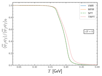
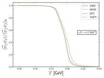
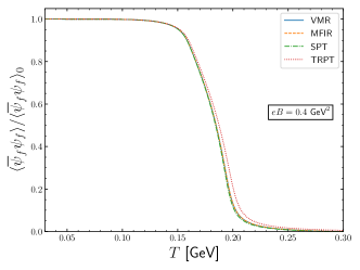
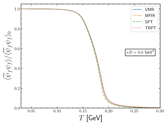
Figure 1: Normalized quark condensate for different magnetic fields as a function of temperature calculated with the different regularization procedures. The quantity $\langle\bar{\psi}_{f}\psi_{f}\rangle_{0}$ represents the quark condensate at $T=0$.

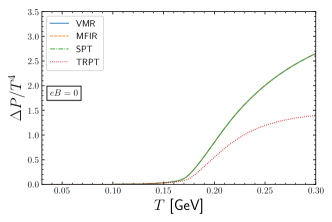
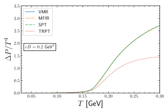
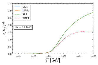
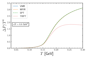
Figure 2: Normalized pressure for different magnetic field values as a function of temperature calculated with the different regularization procedures.

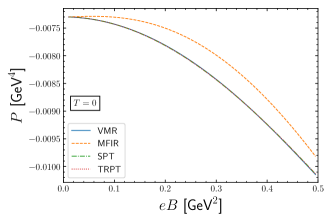
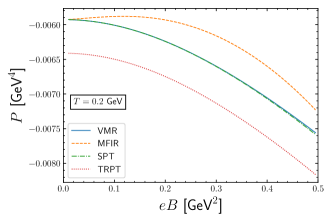
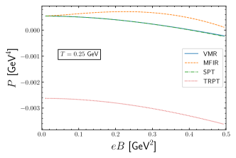
Figure 3: Pressure for different temperature values as a function of $eB$ calculated with the different regularization procedures.

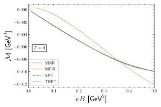
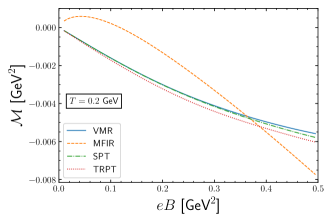
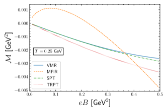
Figure 4: Magnetization for different temperature values as a function of $eB$ calculated with the different regularization procedures.

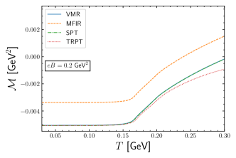
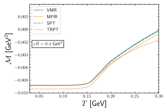
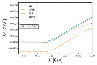
Figure 5: Magnetization for different magnetic field values as a function of the temperature calculated with the different regularization procedures.

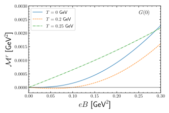
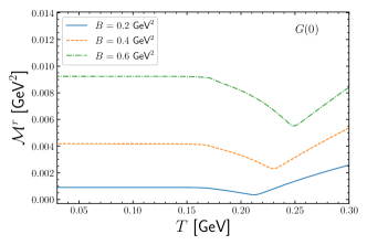
Figure 6: Left panel: renormalized magnetization for a fixed coupling, $G(0)$, at different temperatures as a function of the magnetic field. Right panel: renormalized magnetization for a fixed coupling, $G(0)$, at different magnetic field values as a function of the temperature.

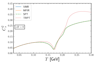
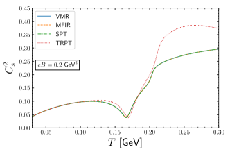
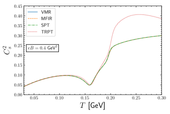
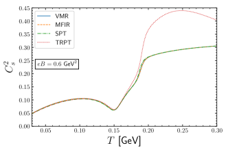
Figure 7: The squared speed of sound for different magnetic field values as a function of temperature calculated with the different regularization procedures

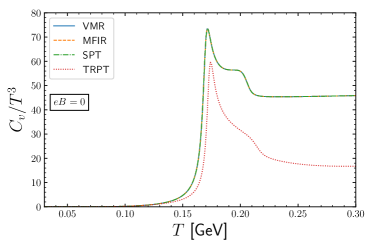
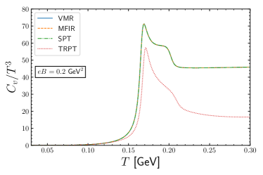
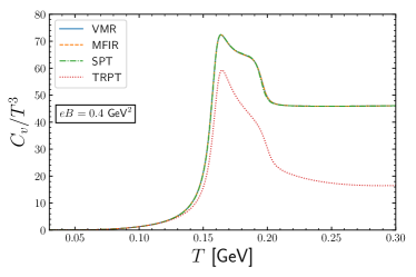
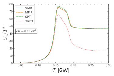
Figure 8: The specific heat for different magnetic field values as a function of temperature calculated with the different regularization procedures.

$eB$ [$\text{GeV}^{2}$]	VMR and MFIR	SPT and TRPT
0.0	5.83200	5.83200
0.2	5.05349	5.19413
0.4	3.74477	4.05506
0.6	2.69719	3.05269

Table 2: $G(B)\Lambda^{2}$ values for the four different regularization prescriptions.

Let us start by analyzing the chiral transition order parameter represented by the quark condensate. Figure 1 shows this quantity as a function of the temperature for different values of the magnetic field illustrating that except for the TRPT all other regularization schemes predict a similar quantitative behavior. As $B$ increases, the TRPT predictions are in better agreement with the ones furnished by the other three prescriptions. It is also clear, from the inflection points, that the pseudocritical temperature value decreases as $B$ increases as one could anticipate. The subtracted pressure, $\Delta P=P(T,B)-P(0,B)$, as a function of $T$ is presented in Fig. 2 for different values of $B$. One can now observe that the TRPT scheme also produces a rather different high-$T$ behavior which is enhanced as higher magnetic fields are considered as the panel for the $eB=0.6\;{\rm GeV}^{2}$ suggests. The maximum at $T\approx 0.23\;{\rm GeV}$ ($eB=0.6\;{\rm GeV}^{2}$) is a reminder that by regulating the (convergent) thermomagnetic integrals one loses predictive power at high temperatures. As already emphasized, a major drawback of this type of regularization procedure is that the Stefan-Boltzmann limit is never attained as $T\to\infty$ [41]. Next, to illustrate the effect of the missing mass-independent terms in the MFIR as well as the effect of regulating the thermomagnetic integrals within the TRPT schemes, we offer Fig. 3. This figure shows that the TRPT predictions become less reliable as $T$ increases, in accordance with our previous discussion. Moreover, the figure clearly illustrates how the neglected mass-independent terms seem to affect the pressure by causing its absolute value to first decrease (at low $B$) and then increase after having reached an extremum. This behavior is in contradiction with the ones predicted by all the other three schemes and directly affects the magnetization as Fig. 4 shows. From the qualitative point of view, it is important to note that the MFIR predicts quark matter to be paramagnetic (${\cal M}>0$) at low $B$ and diamagnetic (${\cal M}<0$) at high magnetic fields, while the other approximations predict it to be diamagnetic (at least up to the highest temperature considered in the figure, $T=0.25\;{\rm GeV}$). The thermal behavior of the magnetization can be better analyzed by plotting this quantity as a function of $T$ for different values of $B$ as Fig. 5 shows. One can observe that the thermal behavior predicted by the MFIR is very sensitive to variations of $B$. At $eB=0.2\;{\rm GeV}^{2}$, the predicted MFIR absolute value for $\cal M$ is lesser than the ones predicted by the other approximations. Then, all the predicted values almost coincide at $eB=0.4\;{\rm GeV}^{2}$ while the MFIR absolute values are higher at $eB=0.6\;{\rm GeV}^{2}$.

At this point, a digression concerning the magnetic character of the QCD vacuum is in order since LQCD evaluations, at $T=0$, have shown that the vacuum is paramagnetic [62] in contradiction to our present findings. The VMR can indeed be reconciled with the LQCD results provided that one uses the same definition for the renormalized magnetization, ${\cal M}^{r}$, used in Ref. [62] where the authors consider

$${\cal M}^{r}\cdot eB={\cal M}\cdot eB-\left.(eB)^{2}\displaystyle{\lim_{eB\to 0}}\frac{{\cal M}\cdot eB}{(eB)^{2}}\right|_{T=0}\,.$$ (18)

In Appendix B, we give the analytical details necessary to obtain this quantity within our framework. Figure 6 shows ${\cal M}^{r}$ varying with the magnetic field (left panel) and with the temperature (right panel) when considering the coupling fixed at the $B=0$ value, $G(0)$. Note that although a fixed coupling does not favor inverse magnetic catalysis, the paramagnetic behavior dominates most regions as the left panel shows. On the other hand, our preliminary investigations suggest that addressing this issue in an appropriate manner will require the determination of how $G$ runs with $B$ with much greater accuracy than the one provided by Ref. [26] (which was adopted here). This nontrivial research programme, which may also require the consideration of strangeness, demands a careful numerical analysis. Therefore, we postpone this investigation for a future application since for our present purposes the results shown in Fig. 6 should convince the reader that the apparent qualitative disagreement between the results shown in Figs 4 and 5 and lattice predictions can indeed be reconciled. For that, one needs to consider the renormalized magnetization, ${\cal M}^{r}$, in conjunction with a coupling which runs with $B$ in a way which is different from the one proposed in Ref. [26]. This last remark is corroborated by the fact that in the extreme $G(0)$ case (no running at all) our VMR predicts quark matter to be paramagnetic in accordance with lattice simulations. Also, when implementing such a programme, one should consider the quark condensates in the vacuum to be $\left\langle\bar{u}u\right\rangle+\left\langle\bar{d}d\right\rangle=-2(0.25\text{GeV})^{3}$ [63].

It is important to emphasize that the VMR scheme proposed here is not totally compatible with the renormalized magnetization. This can be understood by recalling that the purely magnetic contribution guarantees the magnetic catalysis of the VMR gap equation. However, in renormalizable theories such as QED considered by Schwinger [31] or QCD considered in LQCD applications [62], one expects to renormalize the additional $\mathcal{O}(eB)^{2}$ contribution through the term $B^{2}/2$. Therefore, the renormalized magnetization on the PNJL SU(2) model with VMR regularization discussed in Appendix B is merely a projected magnetization that can be a useful tool as far as comparisons with LQCD are concerned. In other words, by doing this, we hope to have a magnetization as similar as possible to that considered in lattice applications [62].

Coming back to Fig. 5 another interesting feature concerns the high-$T$ behavior of the TRPT curves which increase with $T$ in a less linear fashion than all other curves. This could be anticipated based on our previous discussion related to the Stefan-Boltzmann limit. Such a problem becomes even more transparent when one analyzes the speed of sound squared as a function of the temperature. In this case, Fig. 7 clearly reveals that for $T\gtrsim 0.2\,{\rm GeV}$ the TRPT scheme predicts that $C_{s}^{2}$ overshoots the value $1/3$ which is the expected value at the Stefan-Boltzmann limit. The other three methods, on the other hand, predict a steady convergence toward $C_{s}^{2}=1/3$ as $T\to\infty$. Finally, Fig. 8 which shows the specific heat as a function of $T$ for different values of $B$ displays a clear difference between the deconfinement (first peak) and the chiral (second peak) crossover taking place within the $T\sim 0.15-0.2\ {\rm GeV}$ range. One observes a rather good agreement between the full MFIR, VMR, and SPT prescriptions even when the magnetic field reaches high values. On the other hand, the TRPT prescription predicts much lower values when compared to the other regularization schemes especially for temperatures around and above the deconfinement pseudocritical transition. This appears to be yet another consequence of regulating the convergent thermomagnetic integrals within this model (a byproduct of underestimating the Stefan-Boltzmann limit in the pressure). For all regularization prescriptions adopted in this work, one can observe the presence of two peaks in the specific heat as a function of the temperature: the first one (more abrupt) determines the pseudocritical temperature for deconfinement, and the second (smoother) determines the pseudocritical temperature for chiral symmetry restoration. It is important to note that all of our results include IMC through $G(B)$ in the deconfinement and chiral transitions and the splitting between these pseudocritical temperatures remains almost constant if we increase the strength of the magnetic field as already reported in the context of the SU(3) PNJL [64]. This is in the opposite behavior when compared with results of SU(3) PNJL and SU(2) LSM [65, 66], where the splitting increases with $B$. The LQCD study [67] gives further support to the behavior found in Ref.[64].

V Conclusions

We have considered the two-flavor PNJL model in the presence of a thermomagnetic background within the mean field framework in order to compare four different regularization prescriptions. In nonrenormalizable theories, the adoption of different regularization schemes may lead to rather different predictions when a magnetic field and thermal bath are present since one lacks further constraints such as the ones available to renormalizable theories (e.g., renormalization group equations). Apart from considering the three popular schemes represented by the SPT, TRPT, and MFIR, we have proposed an alternative procedure (dubbed VMR). Within this scheme, all divergences are first disentangled and then regulated without any further subtractions while the finite thermomagnetic contribution is integrated over the full momentum range. Comparing the behavior of different physical observables we are able to conclude that, as expected, the TRPT fails to converge to the Stefan-Boltzmann limit when high temperatures are considered. The other three prescriptions predict similar behaviors for the quark condensate, normalized pressure, speed of sound, and specific heat. Nevertheless, the MFIR displays a rather different behavior with regard to the absolute pressure and magnetization. In particular, the MFIR predictions for the latter quantity are in qualitative disagreement with the other three methods. Namely, while the SPT, TRPT, and VMR predict quark matter to be diamagnetic at the $T$, $B$ range analyzed here, the MFIR predicts it to be paramagnetic at low $B$ and diamagnetic at high field values. We believe that this different behavior is due to the missing field-dependent terms subtracted during the MFIR renormalization process. On the other hand, the results furnished by the SPT and the VMR, proposed here, are very similar both qualitatively and quantitatively. The small differences between both schemes only become apparent when examining the results for the magnetization at high field values. This probably happens because within the VMR the divergences contained in the vacuum and in the purely magnetic part have been properly isolated and regulated allowing for the sum over LL to be performed in a closed analytical form. In the view of these results, one may conclude that the VMR offers the most versatile regularization scheme to describe most observables related to magnetized quark matter. We have also observed that, in a scenario without inverse magnetic catalysis, the paramagnetic character of QCD can be properly achieved if one makes use of the renormalized magnetization applied to the VMR scheme.

Appendix A Vacuum Magnetic Regularization

Let us consider the (entangled) vacuum-magnetic parts of the thermodymanical potential as it appears in the lhs of Eq.(10),

$$I=\sum_{f=u,d}\frac{N_{c}}{8\pi^{2}}\int_{\frac{1}{\Lambda^{2}}}^{\infty}ds\frac{e^{-M^{2}s}}{s^{3}}\left(|q_{f}|Bs\coth(|q_{f}|Bs)\right),$$ (19)

where we have used a simple change of variables. Note that the integral is clearly divergent for $s\to 0$. Within the VMR, we first separate the integrand of Eq.(19) into a divergent and a finite part [31] as $s\to 0$. With this aim, let us first expand the $\coth(|q_{f}|Bs)$ in Taylor series, such that

$$\frac{e^{-M^{2}s}}{s^{3}}\left(|q_{f}|Bs\coth(|q_{f}|Bs)\right)=\frac{e^{-M^{2}s}}{s^{3}}\left(1+\frac{(|q_{f}|Bs)^{2}}{3}-\frac{(|q_{f}|Bs)^{4}}{45}+\mathcal{O}((|q_{f}|Bs)^{6})\right),\quad(|q_{f}|Bs)<\pi\,.$$ (20)

As we can see, the first two terms in Eq.(20) are divergent for $s\to 0$ and need regularization, so we can rewrite $I$ as

$$I=I_{0}+I_{field}+I_{int},$$ (21)

where

$$I_{0}=\frac{N_{f}N_{c}}{8\pi^{2}}\int_{\frac{1}{\Lambda^{2}}}^{\infty}ds\frac{e^{-M^{2}s}}{s^{3}}\,$$ (22)

and

$$I_{field}=\sum_{f=u,d}N_{c}\frac{(|q_{f}|B)^{2}}{24\pi^{2}}\int_{\frac{1}{\Lambda^{2}}}^{\infty}ds\frac{e^{-M^{2}s}}{s}\,.$$ (23)

The integral represented by Eq. (23) can be further simplified by considering its explicit solution

$$I_{field}=\sum_{f=u,d}N_{c}\frac{(|q_{f}|B)^{2}}{24\pi^{2}}\Gamma\left[0,\frac{M^{2}}{\Lambda^{2}}\right],$$ (24)

where $\Gamma\left[a,z\right]$ is the incomplete gamma function. Expanding the above result in powers of $M^{2}/\Lambda^{2}$, one obtains

$$I_{field}=\sum_{f=u,d}N_{c}\frac{(|q_{f}|B)^{2}}{24\pi^{2}}\left[-\ln\left(\frac{M^{2}}{\Lambda^{2}}\right)-\gamma_{E}+\frac{M^{2}}{\Lambda^{2}}+\mathcal{O}(M^{4}/\Lambda^{4})\right]\,,$$ (25)

which allows us to identify the divergences and finite terms as $\Lambda\to\infty$. At this limit, all mass-dependent terms vanish so that one only needs to consider

$$I_{field}=\sum_{f=u,d}N_{c}\frac{(|q_{f}|B)^{2}}{24\pi^{2}}\left[-\ln\left(\frac{M^{2}}{\Lambda^{2}}\right)-\gamma_{E}\right]\,.$$ (26)

This last step guarantees that the gap equation will be consistent for the following reason. Deriving $I_{field}$ with respect to $M$, as given by the original Eq. (23), yields

$$\frac{\partial I_{field}}{\partial M}=-\sum_{f=u,d}N_{c}\frac{(|q_{f}|B)^{2}}{12\pi^{2}}M\int_{\frac{1}{\Lambda^{2}}}^{\infty}dse^{-M^{2}s}\,,$$ (27)

which would contribute to the gap equation. However, since this term is finite, one may replace $1/\Lambda^{2}\to 0$ in the lower limit of the integral to get

$$\frac{\partial I_{field}}{\partial M}=-\sum_{f=u,d}N_{c}\frac{(|q_{f}|B)^{2}}{12\pi^{2}M}\,.$$ (28)

This is exactly the same result that one obtains by deriving the truncated $I_{field}$ contribution, Eq. (26), with respect to $M$. Therefore, it is Eq. (26) and not Eq. (23) the one which should be considered when evaluating the thermodynamical potential.

The finite pure magnetic contribution $I_{int}$ is

$$I_{int}=\sum_{f=u,d}\frac{N_{c}}{8\pi^{2}}\int_{0}^{\infty}ds\frac{e^{-M^{2}s}}{s^{3}}\left(|q_{f}|Bs\coth(|q_{f}|Bs)-1-\frac{(|q_{f}|Bs)^{2}}{3}\right).$$ (29)

Now, we can solve the finite integral (29) using the representation of the gamma function,

$$\frac{\Gamma(n+1)}{(\beta)^{n+1}}=\int_{0}^{\infty}~{}dss^{n}e^{-\beta s}\,,$$ (30)

and the Hurwitz-Rieman-zeta function [68],

$$\zeta\left(z,q\right)=\sum_{k=0}^{\infty}\frac{1}{\left(q+k\right)^{z}}\,,$$ (31)

such that

$$I_{int} =\sum_{f=u,d}N_{c}\lim_{\epsilon\rightarrow 0}\frac{(|q_{f}|B)^{2}}{8\pi^{2}}\int_{0}^{\infty}ds~{}e^{-\frac{M^{2}}{|q_{f}|B}s}s^{-3+\epsilon}\left(s\coth(s)-1-\frac{s^{2}}{3}\right)$$

$$=\sum_{f=u,d}N_{c}\frac{(|q_{f}|B)^{2}}{8\pi^{2}}\lim_{\epsilon\rightarrow 0}\left[\Gamma(-1+\epsilon)\left(2^{2-\epsilon}\zeta(-1+\epsilon,\frac{M^{2}}{2|q_{f}|B})-\left(\frac{M^{2}}{|q_{f}|B}\right)^{1-\epsilon}\right)-\frac{\Gamma(-2+\epsilon)}{\left(\frac{M^{2}}{|q_{f}|B}\right)^{-2+\epsilon}}-\frac{1}{3}\frac{\Gamma(\epsilon)}{\left(\frac{M^{2}}{|q_{f}|B}\right)^{\epsilon}}\right].$$ (32)

Make use of some expansions such as $a^{-\epsilon}\cong 1-\ln a~{}\epsilon+\mathcal{O}(\epsilon)$ and

$$\Gamma(-n+\epsilon)=\frac{(-1)^{n}}{n!}\left[\frac{1}{\epsilon}+\psi_{1}(n+1)+\mathcal{O}(\epsilon)\right],$$ (33)

where $\psi_{1}(n+1)=1+\frac{1}{2}+...+\frac{1}{n}-\gamma_{E}$, and $\gamma_{E}=0.577216$ is the Euler-Mascheroni constant. After some algebraic steps, we then obtain

$$I_{int}=-N_{c}\sum_{f=u,d}\frac{(|q_{f}|B)^{2}}{2\pi^{2}}\left[\zeta^{\prime}(-1,x_{f})-\frac{1}{2}(x_{f}^{2}-x_{f})\ln x_{f}~{}+\frac{x_{f}^{2}}{4}-\frac{1}{12}(1+\ln x_{f})\right],$$ (34)

where we have defined $x_{f}=M^{2}/(2|q_{f}|B)$ so that Eq. (21) is exactly the rhs of Eq. (10). Now adding $I_{field}$ as given by the truncated relation, Eq. (26), to $I_{int}$ as given by Eq. (34) allows us to merge two mass-dependent logarithmic terms into a mass-independent one. Namely, $-\ln(M^{2}/\Lambda^{2})+\ln x_{f}=\ln[\Lambda^{2}/(2|q_{f}|B)]$ which does not contribute to the gap equation. Then, Eq.(10) can be finally written as

$$\begin{split}\frac{N_{c}}{8\pi^{2}}\sum_{q_{f}=u,d}(|q_{f}|B)^{2}\int_{\frac{|q_{f}|B}{\Lambda^{2}}}^{\infty}\frac{ds}{s^{2}}e^{-\frac{M^{2}s}{|q_{f}|B}}\coth(s)=&\frac{N_{c}N_{f}}{8\pi^{2}}\int_{\frac{1}{\Lambda^{2}}}^{\infty}\frac{ds}{s^{3}}e^{-M^{2}s}+\frac{N_{c}}{24\pi^{2}}\sum_{q_{f}=u,d}(|q_{f}|B)^{2}\left[\ln\left(\frac{\Lambda^{2}}{2|q_{f}|B}\right)+1-\gamma_{E}\right]\\ &-N_{c}\sum_{f=u,d}\dfrac{(|q_{f}|B)^{2}}{2\pi^{2}}\left[\zeta^{\prime}\left(-1,x_{f}\right)-\left[x_{f}^{2}-x_{f}\right]\frac{\ln x_{f}}{2}+\dfrac{x_{f}^{2}}{4}\right].\end{split}$$ (35)

Appendix B Renormalized Magnetization

The magnetization (${\cal M}^{r}$) considered in lattice evaluations [62], defined by Eq. (18), is the renormalized one. However, contrary to QCD, the PNJL model considered here represents a nonrenormalizable theory. Nevertheless, it is possible to define within the PNJL framework a quantity analogous to ${\cal M}^{r}$ in the following way. First, recall that in lattice QCD applications, the thermodynamical quantities are renormalized in a way to eliminate the contributions of order $\mathcal{O}(eB^{2})$ when $T=0$. Then, using the on shell scheme, one can define the operator

$${\cal P}[X]=\left.(eB)^{2}\lim_{eB\rightarrow 0}\frac{X}{(eB)^{2}}\right|_{T=0}\,,$$ (36)

so that, for a renormalized quantity, one has

$$X^{r}=({1-{\cal P}})[X]\,.$$ (37)

Within the PNJL theory, we first need to evaluate the limit $eB\rightarrow 0$ for each quantity in the VMR thermodynamical potential, Eq.(11). In this case, the thermomagnetic contribution is obviously zero, following the definition given by Eq. (36). Next, let us show that the pure magnetic contribution also does not contribute in this limit. To this end, let us first consider the expansion of the Hurwitz zeta function, $\zeta^{\prime}(-1,x_{f})$ [56], in the limit $eB\rightarrow 0$. This is given by

$$\zeta^{\prime}(-1,x_{f})=\frac{1}{12}-\frac{x_{f}^{2}}{4}+\left(\frac{1}{12}-\frac{x_{f}}{2}+\frac{x_{f}^{2}}{2}\right)\ln x_{f}+\mathcal{O}(x_{f}^{-2}).$$ (38)

Substituting Eq. (38) in the (finite) purely magnetic contribution $I_{int}$ given by Eq. (34), one finds

$$(eB)^{2}\lim_{eB\rightarrow 0}\frac{I_{int}}{(eB)^{2}}=0.$$ (39)

The only remaining magnetic contribution to $\Omega_{VMR}$ is given by $I_{field}$, Eq. (26). We then apply Eq. (36) to the VMR pressure, $P_{VMR}=-\Omega_{VMR}(M,\Phi,T,B)\mid_{M}$, obtaining our “renormalized” pressure

$$P_{VMR}^{r}=P_{VMR}-(eB)^{2}\lim_{eB\rightarrow 0}\frac{P_{VMR}}{(eB)^{2}}\Bigr{|}_{T=0}\,,$$ (40)

which yields

$$P_{VMR}^{r}=P_{VMR}-\sum_{f=u,d}(|q_{f}|B)^{2}\frac{1}{8\pi^{2}}\left(\ln\frac{M(0)^{2}}{\Lambda^{2}}+\gamma_{E}\right).$$ (41)

Finally, our “renormalized” magnetization ${\cal M}^{r}$ can be directly evaluated as

$${\cal M}^{r}=\frac{\partial P^{r}_{VMR}}{\partial B}\;.$$ (42)

References

- Duncan and Thompson [1992] R. C. Duncan and C. Thompson, Astrophys. J. Lett. 392, L9 (1992).
- Fukushima et al. [2008] K. Fukushima, D. E. Kharzeev, and H. J. Warringa, Phys. Rev. D 78, 074033 (2008), arXiv:0808.3382 [hep-ph] .
- Kharzeev and Warringa [2009] D. E. Kharzeev and H. J. Warringa, Phys. Rev. D 80, 034028 (2009), arXiv:0907.5007 [hep-ph] .
- Kharzeev [2009] D. E. Kharzeev, Nucl. Phys. A 830, 543C (2009), arXiv:0908.0314 [hep-ph] .
- Bali et al. [2012a] G. Bali, F. Bruckmann, G. Endrődi, Z. Fodor, S. Katz, and A. Schäfer, Phys. Rev. D 86, 071502 (2012a), arXiv:1206.4205 [hep-lat] .
- Bandyopadhyay and Farias [2020] A. Bandyopadhyay and R. L. Farias, (2020), arXiv:2003.11054 [hep-ph] .
- D’Elia et al. [2010] M. D’Elia, S. Mukherjee, and F. Sanfilippo, Phys. Rev. D 82, 051501 (2010), arXiv:1005.5365 [hep-lat] .
- D’Elia and Negro [2011] M. D’Elia and F. Negro, Phys. Rev. D 83, 114028 (2011), arXiv:1103.2080 [hep-lat] .
- Ilgenfritz et al. [2012] E.-M. Ilgenfritz, M. Kalinowski, M. Muller-Preussker, B. Petersson, and A. Schreiber, Phys. Rev. D 85, 114504 (2012), arXiv:1203.3360 [hep-lat] .
- Endrődi et al. [2019] G. Endrődi, M. Giordano, S. D. Katz, T. Kovács, and F. Pittler, JHEP 07, 007 (2019), arXiv:1904.10296 [hep-lat] .
- Nambu and Jona-Lasinio [1961a] Y. Nambu and G. Jona-Lasinio, Phys. Rev. 122, 345 (1961a).
- Nambu and Jona-Lasinio [1961b] Y. Nambu and G. Jona-Lasinio, Phys. Rev. 124, 246 (1961b).
- Scavenius et al. [2001] O. Scavenius, A. Mocsy, I. Mishustin, and D. Rischke, Phys. Rev. C 64, 045202 (2001), arXiv:nucl-th/0007030 .
- Fraga and Mizher [2008] E. S. Fraga and A. J. Mizher, Phys. Rev. D 78, 025016 (2008), arXiv:0804.1452 [hep-ph] .
- Ratti et al. [2006] C. Ratti, M. A. Thaler, and W. Weise, Phys. Rev. D 73, 014019 (2006), arXiv:hep-ph/0506234 .
- Schaefer et al. [2010] B.-J. Schaefer, M. Wagner, and J. Wambach, Phys. Rev. D 81, 074013 (2010), arXiv:0910.5628 [hep-ph] .
- Fukushima and Hidaka [2013] K. Fukushima and Y. Hidaka, Phys. Rev. Lett. 110, 031601 (2013), arXiv:1209.1319 [hep-ph] .
- Farias et al. [2014] R. Farias, K. Gomes, G. Krein, and M. Pinto, Phys. Rev. C 90, 025203 (2014), arXiv:1404.3931 [hep-ph] .
- Ferrer et al. [2015] E. Ferrer, V. de la Incera, and X. Wen, Phys. Rev. D 91, 054006 (2015), arXiv:1407.3503 [nucl-th] .
- Ayala et al. [2018] A. Ayala, C. Dominguez, S. Hernández-Ortiz, L. Hernández, M. Loewe, D. Manreza Paret, and R. Zamora, Phys. Rev. D 98, 031501 (2018), arXiv:1805.08198 [hep-ph] .
- Ayala et al. [2017] A. Ayala, L. Hernández, M. Loewe, A. Raya, J. Rojas, and R. Zamora, Phys. Rev. D 96, 034007 (2017), arXiv:1706.04956 [hep-ph] .
- Ayala et al. [2016a] A. Ayala, C. Dominguez, L. Hernández, M. Loewe, A. Raya, J. Rojas, and C. Villavicencio, Phys. Rev. D 94, 054019 (2016a), arXiv:1603.00833 [hep-ph] .
- Ayala et al. [2016b] A. Ayala, C. Dominguez, L. Hernández, M. Loewe, and R. Zamora, Phys. Lett. B 759, 99 (2016b), arXiv:1510.09134 [hep-ph] .
- Ayala et al. [2015] A. Ayala, C. Dominguez, L. Hernández, M. Loewe, and R. Zamora, Phys. Rev. D 92, 096011 (2015), [Addendum: Phys.Rev.D 92, 119905 (2015)], arXiv:1509.03345 [hep-ph] .
- Farias et al. [2017] R. Farias, V. Timóteo, S. Avancini, M. Pinto, and G. Krein, Eur. Phys. J. A 53, 101 (2017), arXiv:1603.03847 [hep-ph] .
- Endrődi and Markó [2019] G. Endrődi and G. Markó, JHEP 08, 036 (2019), arXiv:1905.02103 [hep-lat] .
- Ferreira et al. [2014a] M. Ferreira, P. Costa, O. Lourenço, T. Frederico, and C. Providência, Phys. Rev. D 89, 116011 (2014a), arXiv:1404.5577 [hep-ph] .
- Ferreira et al. [2014b] M. Ferreira, P. Costa, D. P. Menezes, C. Providência, and N. Scoccola, Phys. Rev. D 89, 016002 (2014b), [Addendum: Phys.Rev.D 89, 019902 (2014)], arXiv:1305.4751 [hep-ph] .
- Moreira et al. [2020] J. Moreira, P. Costa, and T. E. Restrepo, Phys. Rev. D 102, 014032 (2020), arXiv:2005.07049 [hep-ph] .
- Andersen et al. [2016] J. O. Andersen, W. R. Naylor, and A. Tranberg, Rev. Mod. Phys. 88, 025001 (2016), arXiv:1411.7176 [hep-ph] .
- Schwinger [1951] J. S. Schwinger, Phys. Rev. 82, 664 (1951).
- Costa et al. [2010a] P. Costa, H. Hansen, M. Ruivo, and C. de Sousa, Phys. Rev. D 81, 016007 (2010a), arXiv:0909.5124 [hep-ph] .
- Ruivo et al. [2010] M. Ruivo, P. Costa, H. Hansen, and C. de Sousa, AIP Conf. Proc. 1257, 681 (2010), arXiv:1001.3077 [hep-ph] .
- Costa et al. [2010b] P. Costa, M. Ruivo, C. de Sousa, and H. Hansen, Symmetry 2, 1338 (2010b), arXiv:1007.1380 [hep-ph] .
- Fayazbakhsh et al. [2012] S. Fayazbakhsh, S. Sadeghian, and N. Sadooghi, Phys. Rev. D 86, 085042 (2012), arXiv:1206.6051 [hep-ph] .
- Avancini et al. [2019a] S. S. Avancini, R. L. Farias, N. N. Scoccola, and W. R. Tavares, Phys. Rev. D 99, 116002 (2019a), arXiv:1904.02730 [hep-ph] .
- Allen et al. [2015] P. G. Allen, A. G. Grunfeld, and N. N. Scoccola, Phys. Rev. D 92, 074041 (2015), arXiv:1508.04724 [hep-ph] .
- Duarte et al. [2016a] D. C. Duarte, P. Allen, R. Farias, P. H. A. Manso, R. O. Ramos, and N. Scoccola, Phys. Rev. D 93, 025017 (2016a), arXiv:1510.02756 [hep-ph] .
- Inagaki et al. [2012] T. Inagaki, D. Kimura, H. Kohyama, and A. Kvinikhidze, Phys. Rev. D 86, 116013 (2012), arXiv:1202.5220 [hep-ph] .
- Buballa [2005] M. Buballa, Physics Reports 407, 205–376 (2005).
- Zhuang et al. [1994] P. Zhuang, J. Hufner, and S. Klevansky, Nucl. Phys. A 576, 525 (1994).
- Fukushima [2004] K. Fukushima, Phys. Lett. B 591, 277 (2004), arXiv:hep-ph/0310121 .
- Bratovic et al. [2013] N. M. Bratovic, T. Hatsuda, and W. Weise, Phys. Lett. B 719, 131 (2013), arXiv:1204.3788 [hep-ph] .
- Moreira et al. [2012] J. Moreira, B. Hiller, A. Osipov, and A. Blin, Int. J. Mod. Phys. A 27, 1250060 (2012), arXiv:1008.0569 [hep-ph] .
- Klevansky and Lemmer [1989] S. Klevansky and R. H. Lemmer, Phys. Rev. D 39, 3478 (1989).
- Ebert and Klimenko [2003] D. Ebert and K. Klimenko, Nucl. Phys. A 728, 203 (2003), arXiv:hep-ph/0305149 .
- Ebert et al. [2000] D. Ebert, K. Klimenko, M. Vdovichenko, and A. Vshivtsev, Phys. Rev. D 61, 025005 (2000), arXiv:hep-ph/9905253 .
- Menezes et al. [2009a] D. Menezes, M. Benghi Pinto, S. Avancini, A. Perez Martinez, and C. Providência, Phys. Rev. C 79, 035807 (2009a), arXiv:0811.3361 [nucl-th] .
- Avancini et al. [2012] S. S. Avancini, D. P. Menezes, M. B. Pinto, and C. Providência, Phys. Rev. D 85, 091901 (2012), arXiv:1202.5641 [hep-ph] .
- Menezes et al. [2009b] D. Menezes, M. Benghi Pinto, S. Avancini, and C. Providência, Phys. Rev. C 80, 065805 (2009b), arXiv:0907.2607 [nucl-th] .
- Avancini et al. [2017] S. S. Avancini, R. L. S. Farias, M. Benghi Pinto, W. R. Tavares, and V. S. Timóteo, Phys. Lett. B 767, 247 (2017), arXiv:1606.05754 [hep-ph] .
- Avancini et al. [2018] S. S. Avancini, V. Dexheimer, R. L. S. Farias, and V. S. Timóteo, Phys. Rev. C 97, 035207 (2018), arXiv:1709.02774 [hep-ph] .
- Avancini et al. [2019b] S. S. Avancini, R. L. Farias, and W. R. Tavares, Phys. Rev. D 99, 056009 (2019b), arXiv:1812.00945 [hep-ph] .
- Coppola et al. [2017] M. Coppola, P. Allen, A. Grunfeld, and N. Scoccola, Phys. Rev. D 96, 056013 (2017), arXiv:1707.03795 [hep-ph] .
- Duarte et al. [2016b] D. C. Duarte, R. Farias, P. H. Manso, and R. O. Ramos, J. Phys. Conf. Ser. 706, 052010 (2016b).
- Endrődi [2013] G. Endrődi, JHEP 04, 023 (2013), arXiv:1301.1307 [hep-ph] .
- Fukushima and Sasaki [2013] K. Fukushima and C. Sasaki, Prog. Part. Nucl. Phys. 72, 99 (2013), arXiv:1301.6377 [hep-ph] .
- Ratti et al. [2007] C. Ratti, S. Roessner, M. Thaler, and W. Weise, Eur. Phys. J. C 49, 213 (2007), arXiv:hep-ph/0609218 .
- Schaefer et al. [2007] B.-J. Schaefer, J. M. Pawlowski, and J. Wambach, Phys. Rev. D 76, 074023 (2007), arXiv:0704.3234 [hep-ph] .
- Gamayun et al. [2012] O. Gamayun, E. Gorbar, and V. Gusynin, Phys. Rev. D 86, 065021 (2012), arXiv:1206.2266 [hep-ph] .
- Cao et al. [2014] G. Cao, L. He, and P. Zhuang, Phys. Rev. D 90, 056005 (2014), arXiv:1408.5364 [hep-ph] .
- Bali et al. [2013] G. Bali, F. Bruckmann, G. Endrődi, F. Gruber, and A. Schäefer, JHEP 04, 130 (2013), arXiv:1303.1328 [hep-lat] .
- Klevansky [1992] S. P. Klevansky, Rev. Mod. Phys. 64, 649 (1992).
- Ferreira et al. [2014c] M. Ferreira, P. Costa, and C. Providência, Phys. Rev. D 90, 016012 (2014c), arXiv:1406.3608 [hep-ph] .
- Ferreira et al. [2014d] M. Ferreira, P. Costa, and C. Providência, Phys. Rev. D 89, 036006 (2014d), arXiv:1312.6733 [hep-ph] .
- Mizher et al. [2010] A. J. Mizher, M. Chernodub, and E. S. Fraga, Phys. Rev. D 82, 105016 (2010), arXiv:1004.2712 [hep-ph] .
- Bali et al. [2012b] G. Bali, F. Bruckmann, G. Endrődi, Z. Fodor, S. Katz, S. Krieg, A. Schafer, and K. Szabo, JHEP 02, 044 (2012b), arXiv:1111.4956 [hep-lat] .
- Gradshteyn and Ryzhik [2007] I. S. Gradshteyn and I. M. Ryzhik, Table of integrals, series, and products, seventh ed. (Elsevier/Academic Press, Amsterdam, 2007).