Certified Robustness of Graph Neural Networks against Adversarial Structural Perturbation

Abstract.

Graph neural networks (GNNs) have recently gained much attention for node and graph classification tasks on graph-structured data. However, multiple recent works showed that an attacker can easily make GNNs predict incorrectly via perturbing the graph structure, i.e., adding or deleting edges in the graph. We aim to defend against such attacks via developing certifiably robust GNNs. Specifically, we prove the certified robustness guarantee of any GNN for both node and graph classifications against structural perturbation. Moreover, we show that our certified robustness guarantee is tight. Our results are based on a recently proposed technique called randomized smoothing, which we extend to graph data. We also empirically evaluate our method for both node and graph classifications on multiple GNNs and multiple benchmark datasets. For instance, on the Cora dataset, Graph Convolutional Network with our randomized smoothing can achieve a certified accuracy of 0.49 when the attacker can arbitrarily add/delete at most 15 edges in the graph.

1. Introduction

Graphs are a powerful tool to represent data from diverse domains such as social networks, biology, finance, security, etc.. Node classification and graph classification are two basic tasks on graphs. Specifically, given a graph, node classification aims to classify nodes in the graph in a semi-supervised fashion, while graph classification aims to assign a label to the entire graph instead of individual nodes. Node and graph classifications have many applications, including but not limited to, profiling users in social networks (Zheleva and Getoor, 2009; Mislove et al., 2010; Gong and Liu, 2016; Jia et al., 2017), classifying proteins (Hamilton et al., 2017; Veličković et al., 2018), and fraud detection (Pandit et al., 2007; Tamersoy et al., 2014; Wang et al., 2017a; Weber et al., 2019; Gong et al., 2014; Wang et al., 2017b, 2018, 2019). Various methods such as label propagation (Zhu et al., 2003), belief propagation (Pearl, 1988), iterative classification (Sen et al., 2008), and graph neural networks (GNNs) (Kipf and Welling, 2017; Hamilton et al., 2017; Gilmer et al., 2017; Veličković et al., 2018; Xu et al., 2018) have been proposed for node/graph classifications. Among them, GNNs have attracted much attention recently because of their expressiveness and superior performance.

However, several recent works (Zügner et al., 2018; Dai et al., 2018; Zügner and Günnemann, 2019a; Bojchevski and Günnemann, 2019a; Wang and Gong, 2019) have demonstrated that an attacker can easily fool GNNs to make incorrect predictions via perturbing 1) the node features and/or 2) the structure of the graph (i.e., adding and/or deleting edges in the graph). Therefore, it is of great importance to develop certifiably robust GNNs against such attacks. A few recent works (Zügner and Günnemann, 2019b; Bojchevski et al., 2020; Jin et al., 2020; Bojchevski and Günnemann, 2019b; Zügner and Günnemann, 2020) study certified robustness of GNNs against node feature or structural perturbation. However, these methods only focus on certifying robustness for a specific GNN (Zügner and Günnemann, 2019b; Bojchevski and Günnemann, 2019b; Jin et al., 2020; Zügner and Günnemann, 2020) or/and did not formally prove tight robustness guarantees (Bojchevski et al., 2020) in general.

We aim to bridge this gap in this work. Specifically, we aim to provide tight certified robustness guarantees of any GNN classifier against structural perturbations for both node and graph classification. Towards this goal, we leverage a recently developed technique called randomized smoothing (Cao and Gong, 2017; Liu et al., 2018; Lecuyer et al., 2019; Li et al., 2019; Cohen et al., 2019; Jia et al., 2020a), which can turn any base classifier (e.g., a GNN classifier in our problem) to a robust one via adding random noise to a testing example (i.e., a graph in our problem). A classifier is certifiably robust if it provably predicts the same label when the attacker adds/deletes at most $K$ edges in the graph, where we call $K$ certified perturbation size.

Graph structures are binary data, i.e., a pair of nodes can be either connected or unconnected. Therefore, we develop randomized smoothing for binary data and leverage it to obtain certified robustness of GNNs against structural perturbation. First, we theoretically derive a certified perturbation size for any GNN classifier with randomized smoothing via addressing several challenges. For instance, we divide the graph structure space into regions in a novel way such that we can apply the Neyman-Pearson Lemma (Neyman and Pearson, 1933) to certify robustness. We also prove that our derived certified perturbation size is tight if no assumptions on the GNN classifier are made.

Second, we design a method to compute our certified perturbation size in practice. It is challenging to compute our certified perturbation size as it involves estimating probability bounds simultaneously and solving an optimization problem. To address the challenge, we first adopt the simultaneous confidence interval estimation method (Jia et al., 2020a) to estimate the probability bounds with probabilistic guarantees. Then, we design an algorithm to solve the optimization problem to obtain our certified perturbation size with the estimated probability bounds.

We also empirically evaluate our method. Specifically, for node classification, we consider Graph Convolutional Network (GCN) (Kipf and Welling, 2017) and Graph Attention Network (GAT) (Veličković et al., 2018) on several benchmark datasets including Cora, Citeseer, and Pubmed (Sen et al., 2008). For graph classification, we consider Graph Isomorphism Network (GIN) (Xu et al., 2019b) on benchmark datasets including MUTAG, PROTEINS, and IMDB (Yanardag and Vishwanathan, 2015). For instance, on the Cora dataset, GCN with our randomized smoothing can achieve certified accuracies of 0.55, 0.50, and 0.49 when the attacker arbitrarily adds/deletes at most 5, 10, and 15 edges, respectively. On the MUTAG dataset, GIN with our randomized smoothing can achieve certified accuracies of 0.45, 0.45, and 0.40 when the attacker arbitrarily adds/deletes at most 5, 10, and 15 edges, respectively.

Our major contributions can be summarized as follows:

• We prove the certified robustness guarantee of any GNN against structural perturbation. Moreover, we show that our certified robustness guarantee is tight.

• Our certified perturbation size is the solution to an optimization problem and we design an algorithm to solve the problem.

• We empirically evaluate our method for both node and graph classifications on multiple benchmark datasets.

2. Background

2.1. Node Classification vs. Graph Classification

We consider GNNs for both node classification (Kipf and Welling, 2017; Hamilton et al., 2017; Veličković et al., 2018) and graph classification (Hamilton et al., 2017; Xu et al., 2019b). Suppose we are given an undirected graph $G$ with node features.

• Node classification. A node classifier predicts labels for nodes in the graph in a semi-supervised fashion. Specifically, a subset of nodes in $G$ are already labeled, which are called training nodes and denoted as $V_{T}$. A node classifier $f_{n}$ takes the graph $G$ and the training nodes $V_{T}$ as an input and predicts the label for remaining nodes, i.e., $f_{n}(G,V_{T},u)$ is the predicted label for a node $u$.

• Graph classification. A graph classifier aims to predict a label for the entire graph instead of individual nodes, i.e., $f_{g}(G)$ is the predicted label for the graph $G$. Such a graph classifier can be trained using a set of graphs with ground truth labels.

2.2. Adversarial Structural Perturbation

An attacker aims to fool a node classifier or graph classifier to make predictions as the attacker desires via perturbing the graph structure, i.e., deleting some edges and/or adding some edges in the graph (Zügner et al., 2018; Dai et al., 2018; Zügner and Günnemann, 2019a; Bojchevski and Günnemann, 2019a; Wang and Gong, 2019). Since our work focuses on structural perturbation, we treat the node feature matrix and the training nodes as constants. Moreover, we simply write a node classifier $f_{n}(G,V_{T},u)$ or a graph classifier $f_{g}(G)$ as $f(\mathbf{s})$, where the binary vector $\mathbf{s}$ represents the graph structure. Note that a node classifier should also take a node $u$ as input and predict its label. However, we omit the explicit dependency on a node $u$ for simplicity. We call $\mathbf{s}$ structure vector. For instance, $\mathbf{s}$ can be the concatenation of the upper triangular part of the adjacency matrix of the graph (excluding the diagonals) when the attacker can modify the connection status of any pair of nodes, i.e., $\mathbf{s}$ includes the connection status for each pair of nodes in the graph. When the attacker can only modify the connection status between $u$ and each remaining node, $\mathbf{s}$ can also be the $u$th row of the adjacency matrix of the graph (excluding the self-loop $(u,u)$th entry). We assume the structure vector $\mathbf{s}$ has $n$ entries. As we will see, such simplification makes it easier to present our certified robustness against structural perturbation.

We denote by vector $\delta\in\{0,1\}^{n}$ the attacker’s perturbation to the graph structure. Specifically, $\delta_{i}=1$ if and only if the attacker changes the $i$th entry in the structure vector $\mathbf{s}$, i.e., the attacker changes the connection status of the corresponding pair of nodes. Moreover, $\mathbf{s}\oplus\delta$ is the perturbed structure vector, which represents the perturbed graph structure, where $\oplus$ is the XOR operator between two binary variables. We use $||\delta||_{0}$ to measure the magnitude of the adversarial perturbation as it has semantic meanings. Specifically, $||\delta||_{0}$ is the number of node pairs whose connection statuses are modified by the attacker.

3. Certified Robustness

3.1. Randomized Smoothing with Binary Noise

We first define a noise distribution in the discrete structure vector space $\{0,1\}^{n}$. Then, we define a smoothed classifier based on the noise distribution and a node/graph classifier (called base classifier). Specifically, we consider the noise vector $\epsilon$ has the following probability distribution in the discrete space $\{0,1\}^{n}$:

(1) $$\text{Pr}(\epsilon_{i}=0)=\beta,\ \text{Pr}(\epsilon_{i}=1)=1-\beta,$$

where $i=1,2,\cdots,n$. When we add a random noise vector $\epsilon$ to the structure vector $\mathbf{s}$, the $i$th entry of $\mathbf{s}$ is preserved with probability $\beta$ and changed with probability $1-\beta$. In other words, our random noise means that, for each pair of nodes in the graph, we keep its connection status with probability $\beta$ and change its connection status with probability $1-\beta$. Based on the noise distribution and a base node/graph classifier $f(\mathbf{s})$, we define a smoothed classifier $g(\mathbf{s})$ as follows:

(2) $$g(\mathbf{s})=\operatornamewithlimits{argmax}_{c\in\mathcal{C}}\text{Pr}(f(\mathbf{s}\oplus\epsilon)=c),$$

where $\mathcal{C}$ is the set of labels, $\oplus$ is the XOR operator between two binary variables, $\text{Pr}(f(\mathbf{s}\oplus\epsilon)=c)$ is the probability that the base classifier $f$ predicts label $c$ when we add random noise $\epsilon$ to the structure vector $\mathbf{s}$, and $g(\mathbf{s})$ is the label predicted for $\mathbf{s}$ by the smoothed classifier. Moreover, we note that $g(\mathbf{s}\oplus\delta)$ is the label predicted for the perturbed structure vector $\mathbf{s}\oplus\delta$. Existing randomized smoothing methods (Cao and Gong, 2017; Liu et al., 2018; Lecuyer et al., 2019; Li et al., 2019; Cohen et al., 2019; Jia et al., 2020a) add random continuous noise (e.g., Gaussian noise, Laplacian noise) to a testing example (i.e., the structure vector $\mathbf{s}$ in our case). However, such continuous noise is not meaningful for the binary structure vector.

Our goal is to show that a label is provably the predicted label by the smoothed classifier $g$ for the perturbed structure vector $\mathbf{s}\oplus\delta$ when the $\ell_{0}$-norm of the adversarial perturbation $\delta$, i.e., $\|\delta\|_{0}$, is bounded. Next, we theoretically derive the certified perturbation size $K$, prove the tightness of the certified perturbation size, and discuss how to compute the certified perturbation size in practice.

3.2. Theoretical Certification

3.2.1. Overview

Let $X=\mathbf{s}\oplus\epsilon$ and $Y=\mathbf{s}\oplus\delta\oplus\epsilon$ be two random variables, where $\epsilon$ is the random binary noise drawn from the distribution defined in Equation 1. $X$ and $Y$ represent random structure vectors obtained by adding random binary noise $\epsilon$ to the structure vector $\mathbf{s}$ and its perturbed version $\mathbf{s}\oplus\delta$, respectively.

Suppose, when taking $X$ as an input, the base GNN classifier $f$ correctly predicts the label $c_{A}$ with the largest probability. Then, our key idea is to guarantee that, when taking $Y$ as an input, $f$ still predicts $c_{A}$ with the largest probability. Moreover, we denote $c_{B}$ as the predicted label by $f$ with the second largest probability.

Then, our goal is to find the maximum perturbation size such that the following inequality holds:

(3) $$\text{Pr}(f(Y)=c_{A})>\text{Pr}(f(Y)=c_{B}).$$

Note that it is challenging to compute the probabilities $\text{Pr}(f(Y)=c_{A})$ and $\text{Pr}(f(Y)=c_{B})$ exactly because $f$ is highly nonlinear in practice. To address the challenge, we first derive a lower bound of $\text{Pr}(f(Y)=c_{A})$ and an upper bound of $\text{Pr}(f(Y)=c_{B})$. Then, we require that the lower bound of $\text{Pr}(f(Y)=c_{A})$ is larger than the upper bound of $\text{Pr}(f(Y)=c_{B})$. Specifically, we derive the lower bound and upper bound by constructing certain regions in the graph structure space $\{0,1\}^{n}$ such that the probabilities $Y$ is in these regions can be efficiently computed for any $||\delta||_{0}=k$. Then, we iteratively search the maximum $k$ under the condition that the lower bound is larger than the upper bound. Finally, we treat the maximum $k$ as the certified perturbation size $K$.

3.2.2. Deriving the lower and upper bounds

Our idea is to divide the graph structure space $\{0,1\}^{n}$ into regions in a novel way such that we can apply the Neyman-Pearson Lemma (Neyman and Pearson, 1933) to derive the lower bound and upper bound. First, for any data point $\mathbf{z}\in\{0,1\}^{n}$, we have the density ratio $\frac{\text{Pr}(X=\mathbf{z})}{\text{Pr}(Y=\mathbf{z})}=\big{(}\frac{\beta}{1-\beta}\big{)}^{w-v}$ based on the noise distribution defined in Equation 1, where $w=\|\mathbf{s}-\mathbf{z}\|_{0}$ and $v=\|\mathbf{s}\oplus\delta-\mathbf{z}\|_{0}$ (please refer to Section 7.4 in for details). Therefore, we have the density ratio $\frac{\text{Pr}(X=\mathbf{z})}{\text{Pr}(Y=\mathbf{z})}=\big{(}\frac{\beta}{1-\beta}\big{)}^{m}$ for any $\mathbf{z}\in\{0,1\}^{n}$, where $m=-n,-n+1,\cdots,n-1,n$. Furthermore, we define a region $\mathcal{R}(m)$ as the set of data points whose density ratios are $\big{(}\frac{\beta}{1-\beta}\big{)}^{m}$, i.e., $\mathcal{R}(m)=\{\mathbf{z}\in\{0,1\}^{n}:\frac{\text{Pr}(X=\mathbf{z})}{\text{Pr}(Y=\mathbf{z})}=\big{(}\frac{\beta}{1-\beta}\big{)}^{m}\}$, and we denote by $r(m)$ the corresponding density ratio, i.e., $r(m)=\big{(}\frac{\beta}{1-\beta}\big{)}^{m}$. Moreover, we rank the $2n+1$ regions in a descending order with respect to their density ratios, and denote the ranked regions as $\mathcal{R}_{1},\mathcal{R}_{2},\cdots,\mathcal{R}_{2n+1}$.

Suppose we have a lower bound of the largest label probability $\text{Pr}(f(X)=c_{A})$ for $c_{A}$ and denote it as $\underline{p_{A}}$, and an upper bound of the remaining label probability $\text{Pr}(f(X)=c)$ for $c\neq c_{A}$ and denote it as $\overline{p_{B}}$. Assuming there exist $c_{A}$ and $\underline{p_{A}}$, $\overline{p_{B}}\in[0,1]$ such that

(4) $$\text{Pr}(f(X)=c_{A})\geq\underline{p_{A}}\geq\overline{p_{B}}\geq\max_{c\neq c_{A}}\text{Pr}(f(X)=c).$$

Next, we construct two regions $\mathcal{A}$ and $\mathcal{B}$ such that $\text{Pr}(X\in\mathcal{A})=\underline{p_{A}}$ and $\text{Pr}(X\in\mathcal{B})=\overline{p_{B}}$, respectively. Specifically, we gradually add the regions $\mathcal{R}_{1},\mathcal{R}_{2},\cdots,\mathcal{R}_{2n+1}$ to $\mathcal{A}$ until $\text{Pr}(X\in\mathcal{A})=\underline{p_{A}}$. Moreover, we gradually add the regions $\mathcal{R}_{2n+1},\mathcal{R}_{2n},\cdots,\mathcal{R}_{1}$ to $\mathcal{B}$ until $\text{Pr}(X\in\mathcal{B})=\overline{p_{B}}$. We construct the regions $\mathcal{A}$ and $\mathcal{B}$ in this way such that we can apply the Neyman-Pearson Lemma (Neyman and Pearson, 1933) for them. Formally, we define the regions $\mathcal{A}$ and $\mathcal{B}$ as follows:

(5) $$\mathcal{A}=\bigcup_{j=1}^{a^{\star}-1}\mathcal{R}_{j}\cup\underline{\mathcal{R}_{a^{\star}}}$$

(6) $$\mathcal{B}=\bigcup_{j=b^{\star}+1}^{2n+1}\mathcal{R}_{j}\cup\underline{\mathcal{R}_{b^{\star}}},$$

where

$$a^{\star}=\operatornamewithlimits{argmin}_{a\in\{1,2,\cdots,2n+1\}}a,\ s.t.\ \sum_{j=1}^{a}\textrm{Pr}(X\in\mathcal{R}_{j})\geq\underline{p_{A}},$$

$$b^{\star}=\operatornamewithlimits{argmax}_{b\in\{1,2,\cdots,2n+1\}}b,\ s.t.\ \sum_{j=b}^{2n+1}\textrm{Pr}(X\in\mathcal{R}_{j})\geq\overline{p_{B}}.$$

$\underline{\mathcal{R}_{a^{\star}}}$ is any subregion of $\mathcal{R}_{a^{\star}}$ such that $\text{Pr}(X\in\underline{\mathcal{R}_{a^{\star}}})=\underline{p_{A}}-\sum_{j=1}^{a^{*}-1}\textrm{Pr}(X\in\mathcal{R}_{j})$, and $\underline{\mathcal{R}_{b^{\star}}}$ is any subregion of $\mathcal{R}_{b^{\star}}$ such that $\text{Pr}(X\in\underline{\mathcal{R}_{b^{\star}}})=\overline{p_{B}}-\sum_{j={b^{*}+1}}^{2n+1}\textrm{Pr}(X\in\mathcal{R}_{j})$.

Finally, based on the Neyman-Pearson Lemma, we can derive a lower bound of $\text{Pr}(f(Y)=c_{A})$ and an upper bound of $\text{Pr}(f(Y)=c_{B})$. Formally, we have the following lemma:

Lemma 1.

We have the following bounds:

(7) $$\text{Pr}(f(Y)=c_{A})\geq\text{Pr}(Y\in\mathcal{A}),$$

(8) $$\text{Pr}(f(Y)=c_{B})\leq\text{Pr}(Y\in\mathcal{B}).$$

Proof.

See Section 7.1. ∎

3.2.3. Deriving the certified perturbation size

Given Lemma 1, we can derive the certified perturbation size $K$ as the maximum $k$ such that the following inequality holds for $\forall||\delta||_{0}=k$:

(9) $$\text{Pr}(Y\in\mathcal{A})>\text{Pr}(Y\in\mathcal{B}).$$

Formally, we have the following theorem:

Theorem 1 (Certified Perturbation Size).

Let $f$ be any base node/graph classifier. The random noise vector $\epsilon$ is defined in Equation 1. The smoothed classifier $g$ is defined in Equation 2. Given a structure vector $\mathbf{s}\in\{0,1\}^{n}$, suppose there exist $c_{A}$ and $\underline{p_{A}},\overline{p_{B}}\in[0,1]$ that satisfy Equation 4. Then, we have

(10) $$g(\mathbf{s}\oplus\delta)=c_{A},\forall||\delta||_{0}\leq K,$$

where the certified perturbation size $K$ is the solution to the following optimization problem:

(11) $$K=\operatornamewithlimits{argmax}k,$$

(12) $$\textrm{s.t. }\text{Pr}(Y\in\mathcal{A})>\text{Pr}(Y\in\mathcal{B}),\,\forall||\delta||_{0}=k.$$

Proof.

See Section 7.2. ∎

Next, we show that our certified perturbation size is tight in the following theorem.

Theorem 2 (Tightness of the Certified Perturbation Size).

Assume $\underline{p_{A}}\geq\overline{p_{B}}$, $\underline{p_{A}}+\overline{p_{B}}\leq 1$, and $\underline{p_{A}}+(|\mathcal{C}|-1)\cdot\overline{p_{B}}\geq 1$, where $|\mathcal{C}|$ is the number of labels. For any perturbation $\delta$ with $||\delta||_{0}>K$, there exists a base classifier $f^{*}$ consistent with Equation 4 such that $g(\mathbf{s}\oplus\delta)\neq c_{A}$ or there exist ties.

Proof.

See Section 7.3. ∎

We have several observations on our major theorems.

• Our theorems are applicable to any base node/graph classifier. Moreover, although we focus on classifiers on graphs, our theorems are applicable to any base classifier that takes binary features as input.

• Our certified perturbation size $K$ depends on $\underline{p_{A}}$, $\overline{p_{B}}$, and $\beta$. In particular, when the probability bounds $\underline{p_{A}}$ and $\overline{p_{B}}$ are tighter, our certified perturbation size $K$ is larger. We use the probability bounds $\underline{p_{A}}$ and $\overline{p_{B}}$ instead of their exact values, because it is challenging to compute $p_{A}$ and $p_{B}$ exactly.

• When no assumptions on the base classifier are made and randomized smoothing with the noise distribution defined in Equation 1 is used, it is impossible to certify a perturbation size larger than $K$.

3.3. Certification in Practice

Computing our certified perturbation size $K$ in practice faces two challenges. The first challenge is to estimate the probability bounds $\underline{p_{A}}$ and $\overline{p_{B}}$. The second challenge is to solve the optimization problem in Equation 11 to get $K$ with the given $\underline{p_{A}}$ and $\overline{p_{B}}$. We leverage the method developed in (Jia et al., 2020a) to address the first challenge, and we develop an efficient algorithm to address the second challenge.

Estimating $\underline{p_{A}}$ and $\overline{p_{B}}$:  We view the probabilities $p_{1},p_{2},\cdots,p_{|\mathcal{C}|}$ as a multinomial distribution over the label set $\mathcal{C}$. If we sample a noise $\epsilon$ from our noise distribution uniformly at random, then $f(\mathbf{s}\oplus\epsilon)$ can be viewed as a sample from the multinomial distribution. Then, estimating $\underline{p_{A}}$ and $\overline{p_{c}}$ for $c\in\mathcal{C}\setminus\{c_{A}\}$ is essentially a one-sided simultaneous confidence interval estimation problem. In particular, we leverage the simultaneous confidence interval estimation method developed in (Jia et al., 2020a) to estimate these bounds with a confidence level at least $1-\alpha$. Specifically, we sample $d$ random noise, i.e., $\epsilon^{1},\epsilon^{2},\cdots,\epsilon^{d}$, from the noise distribution defined in Equation 1. We denote by $d_{c}$ the frequency of the label $c$ predicted by the base classifier for the $d$ noisy examples. Formally, we have $d_{c}=\sum_{j=1}^{d}\mathbb{I}(f(\mathbf{s}\oplus\epsilon^{j})=c)$ for each $c\in\mathcal{C}$ and $\mathbb{I}$ is the indicator function. Moreover, we assume $c_{A}$ has the largest frequency and the smoothed classifier predicts $c_{A}$ as the label, i.e., $g(\mathbf{s})=c_{A}$. According to (Jia et al., 2020a), we have the following probability bounds with a confidence level at least $1-\alpha$:

(13) $$\underline{p_{A}}=B\left(\frac{\alpha}{|\mathcal{C}|};d_{c_{A}},d-d_{c_{A}}+1\right)$$

(14) $$\overline{p_{c}}=B\left(1-\frac{\alpha}{|\mathcal{C}|};d_{c}+1,d-d_{c}\right),\ \forall c\neq c_{A},$$

where $B(q;u,w)$ is the $q$th quantile of a beta distribution with shape parameters $u$ and $w$. Then, we estimate $\overline{p_{B}}$ as follows:

(15) $$\overline{p_{B}}=\min\left(\max_{c\neq c_{A}}\overline{p_{c}},1-\underline{p_{A}}\right).$$

Computing $K$:  After estimating ${\underline{p_{A}}}$ and $\overline{p_{B}}$, we solve the optimization problem in Equation 11 to obtain $K$. First, we have:

(16) $$\text{Pr}(Y\in\mathcal{A})=\sum_{j=1}^{a^{\star}-1}\text{Pr}(Y\in\mathcal{R}_{j})+(\underline{p_{A}}-\sum_{j=1}^{a^{\star}-1}\text{Pr}(X\in\mathcal{R}_{j}))/r_{a^{\star}},$$

(17) $$\text{Pr}(Y\in\mathcal{B})=\sum_{j=b^{\star}+1}^{2n+1}\text{Pr}(Y\in\mathcal{R}_{j})+(\overline{p_{B}}-\sum_{j=b^{\star}+1}^{2n+1}\text{Pr}(X\in\mathcal{R}_{j}))/r_{b^{\star}},$$

where $r_{a^{\star}}$ and $r_{b^{\star}}$ are the density ratios in the regions $\mathcal{R}_{a^{\star}}$ and $\mathcal{R}_{b^{\star}}$, respectively. Therefore, the key to solve the optimization problem is to compute $\text{Pr}(X\in\mathcal{R}(m))$ and $\text{Pr}(Y\in\mathcal{R}(m))$ for each $m\in\{-n,-n+1,\cdots,n\}$ when $||\delta||_{0}=k$. Specifically, we have:

(18) $$\text{Pr}(X\in\mathcal{R}(m))=\sum_{j=\max\{0,m\}}^{\min\{n,n+m\}}\beta^{n-(j-m)}(1-\beta)^{(j-m)}\cdot t(m,j)$$

(19) $$\text{Pr}(Y\in\mathcal{R}(m))=\sum_{j=\max\{0,m\}}^{\min\{n,n+m\}}\beta^{n-j}(1-\beta)^{j}\cdot t(m,j),$$

where $t(m,j)$ is defined as follows:

(20) $$t(m,j)=\begin{cases}0,&\textrm{ if }(m+k)\textrm{ mod }2\neq 0,\\ 0,&\textrm{ if }2j-m<k,\\ {n-k\choose\frac{2j-m-k}{2}}{k\choose\frac{k-m}{2}},&\textrm{ otherwise. }\end{cases}$$

See Section 7.4 for the details on obtaining Equation 18 and 19. Then, we iteratively find the largest $k$ such that the constraint in Equation 12 is satisfied.

4. Evaluation

Table 1. Dataset statistics.

Dataset		#Nodes	#Edges	#Classes
Node Classification	Cora	2,708	5,429	7
	Citeseer	3,327	4,732	6
	Pubmed	19,717	44,338	3
Dataset		#Graphs	Ave.#Nodes	#Classes
Graph Classification	MUTAG	188	17.9	2
	PROTEINS	1,113	39.1	2
	IMDB	1,500	13.0	3

(a) Cora

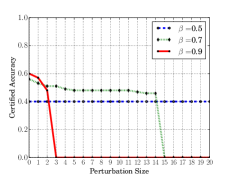
(b) Citeseer

(c) Pubmed

Figure 1. Impact of $\beta$ on the certified accuracy of the smoothed GCN.

(a) Cora

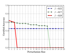
(b) Citeseer

(c) Pubmed

Figure 2. Impact of $\beta$ on the certified accuracy of the smoothed GAT.

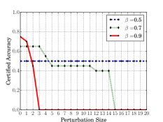
(a) MUTAG

(b) PROTEINS

(c) IMDB

Figure 3. Impact of $\beta$ on the certified accuracy of the smoothed GIN.

4.1. Experimental Setup

We evaluate our method on multiple GNNs and benchmark datasets for both node classification and graph classification.

Benchmark datasets and GNNs:  We use benchmark graphs and GNNs for both node and graph classification. Table 1 shows the statistics of our graphs.

• Node classification: We consider Graph Convolutional Network (GCN) (Kipf and Welling, 2017) and Graph Attention Network (GAT) (Veličković et al., 2018) for node classification. Moreover, we use the Cora, Citeseer, and Pubmed datasets (Sen et al., 2008). They are citation graphs, where nodes are documents and edges indicate citations between documents. In particular, an undirected edge between two documents is created if one document cites the other. The bag-of-words feature of a document is treated as the node feature. Each document also has a label.

• Graph classification: We consider Graph Isomorphism Network (GIN) (Xu et al., 2019b) for graph classification. Moreover, we use the MUTAG, PROTEINS, and IMDB datasets (Yanardag and Vishwanathan, 2015). MUTAG and PROTEINS are bioinformatics datasets. MUTAG contains 188 mutagenic aromatic and heteroaromatic nitro compounds, where each compound represents a graph and each label means whether or not the compound has a mutagenic effect on the Gramnegative bacterium Salmonella typhimurium. PROTEINS is a dataset where nodes are secondary structure elements and there is an edge between two nodes if they are neighbors in the amino-acid sequence or in three-dimensional space. Each protein is represented as a graph and is labeled as enzyme or non-enzyme. IMDB is a movie collaboration dataset. Each graph is an ego-network of an actor/actress, where nodes are actors/actresses and an edge between two actors/actresses indicates that they appear in the same movie. Each graph is obtained from a certain genre of movies, and the task is to classify the genre of a graph.

Training and testing:  For each node classification dataset, following previous works (Kipf and Welling, 2017; Veličković et al., 2018), we sample 20 nodes from each class uniformly at random as the training dataset. Moreover, we randomly sample 100 nodes for testing. For each graph classification dataset, we use 90% of the graphs for training and the remaining 10% for testing, similar to (Xu et al., 2019b).

(a) Smoothed GCN on Cora

(b) Smoothed GIN on MUTAG

Figure 4. Impact of $1-\alpha$ on the certified accuracy of (a) the smoothed GCN and (b) the smoothed GIN.

Parameter setting:  We implement our method in pyTorch. To compute the certified perturbation size, our method needs to specify the noise parameter $\beta$, the confidence level $1-\alpha$, and the number of samples $d$. Unless otherwise mentioned, we set $\beta=0.7$, $1-\alpha=99.9\%$, and $d=10,000$. We also explore the impact of each parameter while fixing the other parameters to the default settings in our experiments. When computing the certified perturbation size for a node $u$ in node classification, we consider an attacker perturbs the connection status between $u$ and the remaining nodes in the graph. We use the publicly available source code for GCN, GAT, and GIN. We use our randomized smoothing to smooth each classifier.

4.2. Experimental Results

Like Cohen et al. (Cohen et al., 2019), we use certified accuracy as the metric to evaluate our method. Specifically, for a smoothed GNN classifier and a given perturbation size, certified accuracy is the fraction of testing nodes (for node classification) or testing graphs (for graph classification), whose labels are correctly predicted by the smoothed classifier and whose certified perturbation size is no smaller than the given perturbation size.

Impact of the noise parameter $\beta$:  Figure 1 and Figure 2 respectively show the certified accuracy of the smoothed GCN and smoothed GAT vs. perturbation size for different $\beta$ on the three node classification datasets. Figure 3 shows the certified accuracy of GIN with randomized smoothing vs. perturbation size for different $\beta$ on the three graph classification datasets.

We have two observations. First, when $\beta=0.5$, the certified accuracy is independent with the perturbation size, which means that an attacker can not attack a smoothed GNN classifier via perturbing the graph structure. This is because $\beta=0.5$ essentially means that the graph is sampled from the space $\{0,1\}^{n}$ uniformly at random. In other words, the graph structure does not contain information about the node labels and a smoothed GNN classifier is reduced to only using the node features. Second, $\beta$ controls a tradeoff between accuracy under no attacks and robustness. Specifically, when $\beta$ is larger, the accuracy under no attacks (i.e., perturbation size is 0) is larger, but the certified accuracy drops more quickly as the perturbation size increases.

Impact of the confidence level $1-\alpha$:  Figure 4a and 4b show the certified accuracy of the smoothed GCN and smoothed GIN vs. perturbation size for different confidence levels, respectively. We observe that as the confidence level $1-\alpha$ increases, the certified accuracy curve becomes slightly lower. This is because a higher confidence level leads to a looser estimation of the probability bound $\underline{p_{A}}$ and $\overline{p_{B}}$, which means a smaller certified perturbation size for a testing node/graph. However, the differences of the certified accuracies between different confidence levels are negligible when the confidence levels are large enough.

Impact of the number of samples $d$:  Figure 5a and 5b show the certified accuracy of the smoothed GCN and smoothed GIN vs. perturbation size for different numbers of samples $d$, respectively. We observe that as the number of samples increases, the certified accuracy curve becomes higher. This is because a larger number of samples makes the estimated probability bound $\underline{p_{A}}$ and $\overline{p_{B}}$ tighter, which means a larger certified perturbation size for a testing node/graph. On Cora, the smoothed GCN achieves certified accuracies of 0.55, 0.50, and 0.49 when $d=50K$ and the attacker arbitrarily adds/deletes at most 5, 10, and 15 edges, respectively. On MUTAG, GIN with our randomized smoothing achieves certified accuracies of 0.45, 0.45, and 0.40 when $d=50K$ and the attacker arbitrarily adds/deletes at most 5, 10, and 15 edges, respectively.

(a) Smoothed GCN on Cora

(b) Smoothed GIN on MUTAG

Figure 5. Impact of $d$ on the certified accuracy of (a) the smoothed GCN and (b) the smoothed GIN.

5. Related Work

We review studies on certified robustness for classifiers on both non-graph data and graph data.

5.1. Non-graph Data

Various methods have been tried to certify robustness of classifiers. A classifier is certifiably robust if it predicts the same label for data points in a certain region around an input example. Existing certification methods leverage Satisfiability Modulo Theories (Scheibler et al., 2015; Carlini et al., 2017; Ehlers, 2017; Katz et al., 2017), mixed integer-linear programming (Cheng et al., 2017; Fischetti and Jo, 2018; Bunel et al., 2018), linear programming (Wong and Kolter, 2018; Wong et al., 2018), semidefinite programming (Raghunathan et al., 2018a, b), dual optimization (Dvijotham et al., 2018a, b), abstract interpretation (Gehr et al., 2018; Mirman et al., 2018; Singh et al., 2018), and layer-wise relaxtion (Weng et al., 2018; Zhang et al., 2018). However, these methods are not scalable to large neural networks and/or are only applicable to specific neural network architectures.

Randomized smoothing (Cao and Gong, 2017; Liu et al., 2018; Lecuyer et al., 2019; Li et al., 2019; Cohen et al., 2019; Salman et al., 2019; Lee et al., 2019; Zhai et al., 2020; Levine and Feizi, 2020; Jia et al., 2020a) was originally developed to defend against adversarial examples. It was first proposed as an empirical defense (Cao and Gong, 2017; Liu et al., 2018). For instance, Cao and Gong (2017) proposed to use uniform random noise from a hypercube centered at an input example to smooth a base classifier. Lecuyer et al. (2019) derived a certified robustness guarantee for randomized smoothing with Gaussian noise or Laplacian noise via differential privacy techniques. Li et al. (2019) leveraged information theory to derive a tighter certified robustness guarantee. Cohen et al. (2019) leveraged the Neyman-Pearson Lemma (Neyman and Pearson, 1933) to obtain a tight certified robustness guarantee under $L_{2}$-norm for randomized smoothing with Gaussian noise. Specifically, they showed that a smoothed classifier verifiably predicts the same label when the $L_{2}$-norm of the adversarial perturbation to an input example is less than a threshold. Salman et al. (2019) designed an adaptive attack against smoothed classifiers and used the attack to train classifiers in an adversarial training paradigm to enlarge the certified robuseness under $L_{2}$-norm. Zhai et al. (2020) proposed to explicitly maximize the certified robustness via a new training strategy. All these methods focused on top-$1$ predictions. Jia et al. (2020a) extended (Cohen et al., 2019) to derive the first certification of top-$k$ predictions against adversarial examples. Compared to other methods for certified robustness, randomized smoothing has two key advantages: 1) it is scalable to large neural networks, and 2) it is applicable to any base classifier.

5.2. Graph Data

Several studies (Dai et al., 2018; Zügner et al., 2018; Zügner and Günnemann, 2019a; Bojchevski and Günnemann, 2019a; Wang and Gong, 2019; Wu et al., 2019; Xu et al., 2019a; Sun et al., 2020; Chang et al., 2020) have shown that attackers can fool GNNs via manipulating the node features and/or graph structure.  (Wu et al., 2019; Xu et al., 2019a; Zhu et al., 2019; Tang et al., 2020; Entezari et al., 2020; Tao et al., 2021) proposed empirical defenses without certified robustness guarantees. A few recent works (Zügner and Günnemann, 2019b; Bojchevski et al., 2020; Jin et al., 2020; Bojchevski and Günnemann, 2019b; Zügner and Günnemann, 2020) study certified robustness of GNNs. Zügner and Günnemann (2019b) considered node feature perturbation. In particular, they derived certified robustness for a particular type of GNN called graph convolutional network (Kipf and Welling, 2017) against node feature perturbation. More specifically, they formulated the certified robustness as a linear programming problem, where the objective is to require that a node’s prediction is constant within an allowable node feature perturbation. Then, they derived the robustness guarantee based on the dual form of the optimization problem, which is motivated by (Wong and Kolter, 2018). (Bojchevski and Günnemann, 2019b; Zügner and Günnemann, 2020; Jin et al., 2020) considered structural perturbation for a specific GNN. Specifically, (Bojchevski and Günnemann, 2019b) required that GNN prediction is a linear function of (personalized) PageRank (Klicpera et al., 2019) and (Zügner and Günnemann, 2020; Jin et al., 2020) could only certify the robustness of GCNs. For example, (Jin et al., 2020) derived the certified robustness of GCN for graph classification via utilizing dualization and convex envelope tools.

Two recent works (Jia et al., 2020b; Bojchevski et al., 2020) leveraged randomized smoothing to provide a model-agnostic certification against structural perturbation. Jia et al. (Jia et al., 2020b) certified the robustness of community detection against structural perturbation. They essentially model the problem as binary classification, i.e., whether a set of nodes are in the same community or not, and design a randomized smoothing technique to certify its robustness. Bojchevski et al. (Bojchevski et al., 2020) generalize the randomized smoothing technique developed in [29] to the sparse setting and derive certified robustness for GNNs. They did not formally prove that their multi-class certificate is tight. However, in the special case of equal flip probabilities, which is equivalent to our certificate, our tightness proof (Theorem 2) applies.

6. Conclusion and Future Work

In this work, we develop the certified robustness guarantee of GNNs for both node and graph classifications against structural perturbation. Our results are applicable to any GNN classifier. Our certification is based on randomized smoothing for binary data which we develop in this work. Moreover, we prove that our certified robustness guarantee is tight when randomized smoothing is used and no assumptions on the GNNs are made. An interesting future work is to incorporate the information of a given GNN to further improve the certified robustness guarantee.

7. Proofs

7.1. Proof of Lemma 1

We first describe the Neyman-Pearson Lemma for binary random variables, which we use to prove Lemma 1.

2

Lemma 1 (Neyman-Pearson Lemma for Binary Random Variables).

Let $X$ and $Y$ be two random variables in the discrete space $\{0,1\}^{n}$ with probability distributions $\textrm{Pr}(X)$ and $\textrm{Pr}(Y)$, respectively. Let $h:\{0,1\}^{n}\rightarrow\{0,1\}$ be a random or deterministic function.

• Let $S_{1}=\{\mathbf{z}\in\{0,1\}^{n}:\frac{\textrm{Pr}(X=\mathbf{z})}{\textrm{Pr}(Y=\mathbf{z})}>r\}$ and $S_{2}=\{\mathbf{z}\in\{0,1\}^{n}:\frac{\textrm{Pr}(X=\mathbf{z})}{\textrm{Pr}(Y=\mathbf{z})}=r\}$ for some $r>0$. Assume $S_{3}\subseteq S_{2}$ and $S=S_{1}\bigcup S_{3}$. If $\textrm{Pr}(h(X)=1)\geq\textrm{Pr}(X\in S)$, then $\textrm{Pr}(h(Y)=1)\geq\textrm{Pr}(Y\in S)$.

• Let $S_{1}=\{\mathbf{z}\in\{0,1\}^{n}:\frac{\textrm{Pr}(X=\mathbf{z})}{\textrm{Pr}(Y=\mathbf{z})}<r\}$ and $S_{2}=\{\mathbf{z}\in\{0,1\}^{n}:\frac{\textrm{Pr}(X=\mathbf{z})}{\textrm{Pr}(Y=\mathbf{z})}=r\}$ for some $r>0$. Assume $S_{3}\subseteq S_{2}$ and $S=S_{1}\bigcup S_{3}$. If $\textrm{Pr}(h(X)=1)\leq\textrm{Pr}(X\in S)$, then $\textrm{Pr}(h(Y)=1)\leq\textrm{Pr}(Y\in S)$.

Proof.

The proof can be found in a standard statistics textbook, e.g., (Lehmann and Romano, 2006). For completeness, we include the proof here. Without loss of generality, we assume that $h$ is random and denote $h(1|z)$ (resp. $h(0|z)$) as the probability that $h(z)=1$ (resp. $h(z)=0)$). We denote $S^{c}$ as the complement of $S$, i.e., $S^{c}=\{0,1\}^{n}\setminus S$. For any $\mathbf{z}\in S$, we have $\frac{\textrm{Pr}(X=\mathbf{z})}{\textrm{Pr}(Y=\mathbf{z})}\geq r$, and for any $\mathbf{z}\in S^{c}$, we have $\frac{\textrm{Pr}(X=\mathbf{z})}{\textrm{Pr}(Y=\mathbf{z})}\leq r$. We prove the first part, and the second part can be proved similarly.

$$\textrm{Pr}(h(Y)=1)-\textrm{Pr}(Y\in S)=$$

$$\sum_{\mathbf{z}\in\{0,1\}^{n}}h(1|\mathbf{z})\textrm{Pr}(Y=\mathbf{z})-\sum_{\mathbf{z}\in S}\textrm{Pr}(Y=\mathbf{z})$$

$$=\Big{(}\sum_{\mathbf{z}\in S^{c}}h(1|\mathbf{z})\textrm{Pr}(Y=\mathbf{z})+\sum_{\mathbf{z}\in S}h(1|\mathbf{z})\textrm{Pr}(Y=\mathbf{z})\Big{)}$$

$$\qquad-\Big{(}\sum_{\mathbf{z}\in S}h(1|\mathbf{z})\textrm{Pr}(Y=\mathbf{z})+\sum_{\mathbf{z}\in S}h(0|\mathbf{z})\textrm{Pr}(Y=\mathbf{z})\Big{)}$$

$$=\sum_{\mathbf{z}\in S^{c}}h(1|\mathbf{z})\textrm{Pr}(Y=\mathbf{z})-\sum_{\mathbf{z}\in S}h(0|\mathbf{z})\textrm{Pr}(Y=\mathbf{z})$$

$$\geq\frac{1}{r}\Big{(}\sum_{\mathbf{z}\in S^{c}}h(1|\mathbf{z})\textrm{Pr}(X=\mathbf{z})-\sum_{\mathbf{z}\in S}h(0|\mathbf{z})\textrm{Pr}(X=\mathbf{z})\Big{)}$$

$$=\frac{1}{r}\Bigg{(}\Big{(}\sum_{\mathbf{z}\in S^{c}}h(1|\mathbf{z})\textrm{Pr}(X=\mathbf{z})+\sum_{\mathbf{z}\in S}h(1|\mathbf{z})\textrm{Pr}(X=\mathbf{z})\Big{)}$$

$$\qquad-\Big{(}\sum_{\mathbf{z}\in S}h(1|\mathbf{z})\textrm{Pr}(X=\mathbf{z})+\sum_{\mathbf{z}\in S}h(0|\mathbf{z})\textrm{Pr}(X=\mathbf{z})\Big{)}\Bigg{)}$$

$$=\frac{1}{r}\Big{(}\sum_{\mathbf{z}\in\{0,1\}^{n}}h(1|\mathbf{z})\textrm{Pr}(X=\mathbf{z})-\sum_{\mathbf{z}\in S}\textrm{Pr}(X=\mathbf{z})\Big{)}$$

$$=\frac{1}{r}\Big{(}\textrm{Pr}(h(X)=1)-\textrm{Pr}(X\in S)\Big{)}$$

$$\geq 0.$$

∎

Next, we restate Lemma 1 and show our proof. See 1

Proof.

Based on the regions $\mathcal{A}$ and $\mathcal{B}$ defined in Equation 5 and Equation 6, we have $\text{Pr}(X\in\mathcal{A})=\underline{p_{A}}$ and $\text{Pr}(X\in\mathcal{B})=\overline{p_{B}}$.

Moreover, based on the conditions in Equation 4, we have:

$$\text{Pr}(f(X)=c_{A})\geq\underline{p_{A}}=\text{Pr}(X\in\mathcal{A});$$

$$\text{Pr}(f(X)=c_{B})\leq\overline{p_{B}}=\text{Pr}(X\in\mathcal{B}).$$

Next, we leverage Lemma 1 to derive the condition for $\text{Pr}(f(Y)=c_{A})>\text{Pr}(f(Y)=c_{B})$. Specifically, we define $h(\mathbf{z})=\mathbb{I}(f(\mathbf{z})=c_{A})$. Then, we have:

$$\text{Pr}(h(X)=1)=\text{Pr}(f(X)=c_{A})\geq\text{Pr}(X\in\mathcal{A}).$$

Moreover, we have $\frac{\text{Pr}(X=\mathbf{z})}{\text{Pr}(Y=\mathbf{z})}>r_{a^{\star}}$ for any $\mathbf{z}\in\bigcup_{j=1}^{a^{\star}-1}\mathcal{R}_{j}$ and $\frac{\text{Pr}(X=\mathbf{z})}{\text{Pr}(Y=\mathbf{z})}=r_{a^{\star}}$ for any $\mathbf{z}\in\underline{\mathcal{R}_{a^{\star}}}$, where $r_{a^{\star}}$ is the probability density ratio in the region $\mathcal{R}_{a^{\star}}$. Therefore, according to the first part of Lemma 1, we have $\text{Pr}(f(Y)=c_{A})\geq\text{Pr}(Y\in\mathcal{A})$. Similarly, based on the second part of Lemma 1, we have $\text{Pr}(f(Y)=c_{B})\leq\text{Pr}(Y\in\mathcal{B})$. ∎

7.2. Proof of Theorem 1

Recall that our goal is to make $\text{Pr}(f(Y)=c_{A})>\text{Pr}(f(Y)=c_{B})$. Based on Lemma 1, it is sufficient to require $\text{Pr}(Y\in\mathcal{A})>\text{Pr}(Y\in\mathcal{B}).$ Therefore, we derive the certified perturbation size $K$ as the maximum $k$ such that the above inequality holds for $\forall||\delta||_{0}=R$.

7.3. Proof of Theorem 2

Our idea is to construct a base classifier $f^{*}$ consistent with the conditions in Equation 4, but the smoothed classifier is not guaranteed to predict $c_{A}$. Let disjoint regions $\mathcal{A}$ and $\mathcal{B}$ be defined as in Equation 5 and Equation 6. We denote $\Gamma=\{1,2,\cdots,c\}\setminus\{c_{A},c_{B}\}$. Then, for each label $c_{i}$ in $\Gamma$, we can find a region $\mathcal{C}_{i}\subseteq\{0,1\}^{n}\setminus(\mathcal{A}\cup\mathcal{B})$ such that $\mathcal{C}_{i}\cap\mathcal{C}_{j}=\emptyset,\forall i,j\in\Gamma,i\neq j$ and $\text{Pr}(X\in\mathcal{C}_{i})\leq\overline{p_{B}}$. We can construct such regions because $\underline{p_{A}}+(|\mathcal{C}|-1)\cdot\overline{p_{B}}\geq 1$. Given those regions, we construct the following base classifier:

$$f^{*}(\mathbf{z})=\begin{cases}c_{A}&\text{if }\mathbf{z}\in\mathcal{A}\\ c_{B}&\text{if }\mathbf{z}\in\mathcal{B}\\ c_{i}&\text{if }\mathbf{z}\in\mathcal{C}_{i}\end{cases}$$

By construction, we have $\text{Pr}(f^{*}(X)=c_{A})=\underline{p_{A}}$, $\text{Pr}(f^{*}(X)=c_{B})=\overline{p_{B}}$, and $\text{Pr}(f^{*}(X)=c_{i})\leq\overline{p_{B}}$ for any $c_{i}\in\Gamma$, which are consistent with Equation 4. From our proof of Theorem 1, we know that when $||\delta||_{0}>K$, we have:

$$\text{Pr}(Y\in\mathcal{A})\leq\text{Pr}(Y\in\mathcal{B}),$$

or equivalently we have:

$$\text{Pr}(f^{*}(Y)=c_{A})\leq\text{Pr}(f^{*}(Y)=c_{B})$$

Therefore, we have either $g(\mathbf{s}\oplus\delta)\neq c_{A}$ or there exist ties when $||\delta||_{0}>K$.

7.4. Computing $\text{Pr}(X\in\mathcal{R}(m))$ and $\text{Pr}(Y\in\mathcal{R}(m))$

We first define the following regions:

$$\mathcal{R}(w,v) =\{\mathbf{z}\in\{0,1\}^{n}:||\mathbf{z}-\mathbf{s}||_{0}=w\text{ and }||\mathbf{z}-\mathbf{s}\oplus\delta||_{0}=v\},$$

for $w,v\in\{0,1,\cdots,n\}$. Intuitively, $\mathcal{R}(w,v)$ includes the binary vectors that are $w$ bits different from $\mathbf{s}$ and $v$ bits different from $\mathbf{s}\oplus\delta$. Next, we compute the size of the region $\mathcal{R}(w,v)$ when $||\delta||_{0}=k$. Without loss of generality, we assume $\mathbf{s}=[0,0,\cdots,0]$ as a zero vector and $\mathbf{s}\oplus\delta=[1,1,\cdots,1,0,0,\cdots,0]$, where the first $k$ entries are 1 and the remaining $n-k$ entries are 0. We construct a binary vector $\mathbf{z}\in\mathcal{R}(w,v)$. Specifically, suppose we flip $i$ zeros in the last $n-k$ zeros in both $\mathbf{s}$ and $\mathbf{s}\oplus\delta$. Then, we flip $w-i$ of the first $k$ bits of $\mathbf{s}$ and flip the rest $k-w+i$ bits of the first $k$ bits of $\mathbf{s}\oplus\delta$. In order to have $\mathbf{z}\in\mathcal{R}(w,v)$, we need $k-w+i+i=v$, i.e., $i=(w+v-k)/2$. Therefore, we have the size $|\mathcal{R}(w,v)|$ of the region $\mathcal{R}(w,v)$ as follows:

$$|\mathcal{R}(w,v)|=\begin{cases}0,&\textrm{ if }(w+v-k)\textrm{ mod }2\neq 0,\\ 0,&\textrm{ if }w+v<k,\\ {n-k\choose\frac{w+v-k}{2}}{k\choose\frac{w-v+k}{2}},&\textrm{ otherwise }\end{cases}$$

Moreover, for each $\mathbf{z}\in\mathcal{R}(w,v)$, we have $\text{Pr}(X=\mathbf{z})=\beta^{n-w}(1-\beta)^{w}$ and $\text{Pr}(Y=\mathbf{z})=\beta^{n-v}(1-\beta)^{v}$. Therefore, we have:

$$\textrm{Pr}(X\in\mathcal{R}(w,v)) =\beta^{n-w}(1-\beta)^{w}\cdot|\mathcal{R}(w,v)|,$$

$$\textrm{Pr}(Y\in\mathcal{R}(w,v)) =\beta^{n-v}(1-\beta)^{v}\cdot|\mathcal{R}(w,v)|.$$

Note that $\mathcal{R}(m)=\cup_{v-w=m}\mathcal{R}(w,v)$. Therefore, we have:

$$\text{Pr}(X\in\mathcal{R}(m))$$

$$= \text{Pr}(X\in\cup_{v-w=m}\mathcal{R}(w,v))$$

$$= \text{Pr}(X\in\cup_{j=\max(0,m)}^{\min(n,n+m)}\mathcal{R}(j-m,j))$$

$$= \sum_{j=\max(0,m)}^{\min(n,n+m)}\text{Pr}(X\in\mathcal{R}(j-m,j))$$

$$= \sum_{j=\max(0,m)}^{\min(n,n+m)}\beta^{n-(j-m)}(1-\beta)^{j-m}\cdot|\mathcal{R}(j-m,j)|$$

$$= \sum_{j=\max(0,m)}^{\min(n,n+m)}\beta^{n-(j-m)}(1-\beta)^{j-m}\cdot t(m,j),$$

where $t(m,j)=|\mathcal{R}(j-m,j)|$.

Similarly, we have

$$\text{Pr}(Y\in\mathcal{R}(m))=\sum_{j=\max(0,m)}^{\min(n,n+m)}\beta^{n-j}(1-\beta)^{j}\cdot t(m,j).$$

Acknowledgements. We thank the anonymous reviewers for their constructive comments. This work is supported by the National Science Foundation under Grants No. 1937786 and 1937787 and the Army Research Office under Grant No. W911NF2110182. Any opinions, findings and conclusions or recommendations expressed in this material are those of the author(s) and do not necessarily reflect the views of the funding agencies.

References

- (1)
- Bojchevski and Günnemann (2019a) Aleksandar Bojchevski and Stephan Günnemann. 2019a. Adversarial Attacks on Node Embeddings via Graph Poisoning. In ICML.
- Bojchevski and Günnemann (2019b) Aleksandar Bojchevski and Stephan Günnemann. 2019b. Certifiable Robustness to Graph Perturbations. In NeurIPS.
- Bojchevski et al. (2020) Aleksandar Bojchevski, Johannes Klicpera, and Stephan Günnemann. 2020. Efficient robustness certificates for discrete data: Sparsity-aware randomized smoothing for graphs, images and more. In ICML.
- Bunel et al. (2018) Rudy R Bunel, Ilker Turkaslan, Philip Torr, Pushmeet Kohli, and Pawan K Mudigonda. 2018. A unified view of piecewise linear neural network verification. In NeurIPS.
- Cao and Gong (2017) Xiaoyu Cao and Neil Zhenqiang Gong. 2017. Mitigating evasion attacks to deep neural networks via region-based classification. In ACSAC.
- Carlini et al. (2017) Nicholas Carlini, Guy Katz, Clark Barrett, and David L Dill. 2017. Provably minimally-distorted adversarial examples. arXiv (2017).
- Chang et al. (2020) Heng Chang, Yu Rong, Tingyang Xu, Wenbing Huang, Honglei Zhang, Peng Cui, Wenwu Zhu, and Junzhou Huang. 2020. A restricted black-box adversarial framework towards attacking graph embedding models. In AAAI.
- Cheng et al. (2017) Chih-Hong Cheng, Georg Nührenberg, and Harald Ruess. 2017. Maximum resilience of artificial neural networks. In ATVA.
- Cohen et al. (2019) Jeremy M Cohen, Elan Rosenfeld, and J Zico Kolter. 2019. Certified adversarial robustness via randomized smoothing. In ICML.
- Dai et al. (2018) Hanjun Dai, Hui Li, Tian Tian, Xin Huang, Lin Wang, Jun Zhu, and Le Song. 2018. Adversarial attack on graph structured data. In ICML.
- Dvijotham et al. (2018a) Krishnamurthy Dvijotham, Sven Gowal, Robert Stanforth, and et al. 2018a. Training verified learners with learned verifiers. arXiv (2018).
- Dvijotham et al. (2018b) Krishnamurthy Dvijotham, Robert Stanforth, Sven Gowal, and et al. 2018b. A Dual Approach to Scalable Verification of Deep Networks.. In UAI.
- Ehlers (2017) Ruediger Ehlers. 2017. Formal verification of piece-wise linear feed-forward neural networks. In ATVA.
- Entezari et al. (2020) Negin Entezari, Saba A Al-Sayouri, Amirali Darvishzadeh, and Evangelos E Papalexakis. 2020. All You Need Is Low (Rank) Defending Against Adversarial Attacks on Graphs. In WSDM.
- Fischetti and Jo (2018) Matteo Fischetti and Jason Jo. 2018. Deep neural networks and mixed integer linear optimization. Constraints (2018).
- Gehr et al. (2018) Timon Gehr, Matthew Mirman, Dana Drachsler-Cohen, Petar Tsankov, Swarat Chaudhuri, and Martin Vechev. 2018. Ai2: Safety and robustness certification of neural networks with abstract interpretation. In IEEE S & P.
- Gilmer et al. (2017) Justin Gilmer, Samuel S Schoenholz, Patrick F Riley, Oriol Vinyals, and George E Dahl. 2017. Neural message passing for quantum chemistry. In ICML.
- Gong et al. (2014) Neil Zhenqiang Gong, Mario Frank, and Prateek Mittal. 2014. Sybilbelief: A semi-supervised learning approach for structure-based sybil detection. IEEE TIFS (2014).
- Gong and Liu (2016) Neil Zhenqiang Gong and Bin Liu. 2016. You are who you know and how you behave: Attribute inference attacks via users’ social friends and behaviors. In USENIX Security Symposium.
- Hamilton et al. (2017) Will Hamilton, Zhitao Ying, and Jure Leskovec. 2017. Inductive representation learning on large graphs. In NIPS.
- Jia et al. (2020a) Jinyuan Jia, Xiaoyu Cao, Binghui Wang, and Neil Zhenqiang Gong. 2020a. Certified Robustness for Top-k Predictions against Adversarial Perturbations via Randomized Smoothing. In ICLR.
- Jia et al. (2020b) Jinyuan Jia, Binghui Wang, Xiaoyu Cao, and Neil Zhenqiang Gong. 2020b. Certified Robustness of Community Detection against Adversarial Structural Perturbation via Randomized Smoothing. In The Web Conference.
- Jia et al. (2017) Jinyuan Jia, Binghui Wang, Le Zhang, and Neil Zhenqiang Gong. 2017. AttriInfer: Inferring user attributes in online social networks using markov random fields. In WWW.
- Jin et al. (2020) Hongwei Jin, Zhan Shi, Venkata Jaya Shankar Ashish Peruri, and Xinhua Zhang. 2020. Certified Robustness of Graph Convolution Networks for Graph Classification under Topological Attacks. In NeurIPS.
- Katz et al. (2017) Guy Katz, Clark Barrett, David L Dill, and et al. 2017. Reluplex: An efficient SMT solver for verifying deep neural networks. In CAV.
- Kipf and Welling (2017) Thomas N Kipf and Max Welling. 2017. Semi-supervised classification with graph convolutional networks. In ICLR.
- Klicpera et al. (2019) Johannes Klicpera, Aleksandar Bojchevski, and Stephan Günnemann. 2019. Predict then propagate: Graph neural networks meet pagerank. In ICLR.
- Lecuyer et al. (2019) Mathias Lecuyer, Vaggelis Atlidakis, Roxana Geambasu, Daniel Hsu, and Suman Jana. 2019. Certified robustness to adversarial examples with differential privacy. In IEEE S & P.
- Lee et al. (2019) GuangHe Lee, Yang Yuan, Shiyu Chang, and Tommi Jaakkola. 2019. Tight Certificates of Adversarial Robustness for Randomly Smoothed Classifiers. In NeurIPS.
- Lehmann and Romano (2006) Erich L Lehmann and Joseph P Romano. 2006. Testing statistical hypotheses. Springer Science & Business Media.
- Levine and Feizi (2020) Alexander Levine and Soheil Feizi. 2020. Robustness Certificates for Sparse Adversarial Attacks by Randomized Ablation. In AAAI.
- Li et al. (2019) Bai Li, Changyou Chen, Wenlin Wang, and Lawrence Carin. 2019. Certified Adversarial Robustness with Additive Noise. NeurIPS.
- Liu et al. (2018) Xuanqing Liu, Minhao Cheng, Huan Zhang, and Cho-Jui Hsieh. 2018. Towards robust neural networks via random self-ensemble. In ECCV.
- Mirman et al. (2018) Matthew Mirman, Timon Gehr, and Martin Vechev. 2018. Differentiable abstract interpretation for provably robust neural networks. In ICML.
- Mislove et al. (2010) Alan Mislove, Bimal Viswanath, Krishna P Gummadi, and Peter Druschel. 2010. You are who you know: inferring user profiles in online social networks. In WSDM.
- Neyman and Pearson (1933) Jerzy Neyman and Egon Sharpe Pearson. 1933. IX. On the problem of the most efficient tests of statistical hypotheses. (1933).
- Pandit et al. (2007) Shashank Pandit, Horng Chau, Samuel Wang, and Christos Faloutsos. 2007. Netprobe: a fast and scalable system for fraud detection in online auction networks. In WWW.
- Pearl (1988) Judea Pearl. 1988. Probabilistic Reasoning in Intelligent Systems: Networks of Plausible Inference. Morgan Kaufmann.
- Raghunathan et al. (2018a) Aditi Raghunathan, Jacob Steinhardt, and Percy Liang. 2018a. Certified defenses against adversarial examples. In ICLR.
- Raghunathan et al. (2018b) Aditi Raghunathan, Jacob Steinhardt, and Percy S Liang. 2018b. Semidefinite relaxations for certifying robustness to adversarial examples. In NeurIPS.
- Salman et al. (2019) Hadi Salman, Jerry Li, Ilya Razenshteyn, Pengchuan Zhang, Huan Zhang, Sebastien Bubeck, and Greg Yang. 2019. Provably robust deep learning via adversarially trained smoothed classifiers. In NeurIPS.
- Scheibler et al. (2015) Karsten Scheibler, Leonore Winterer, Ralf Wimmer, and Bernd Becker. 2015. Towards Verification of Artificial Neural Networks.. In MBMV.
- Sen et al. (2008) Prithviraj Sen, Galileo Namata, Mustafa Bilgic, and et al. 2008. Collective classification in network data. AI magazine (2008).
- Singh et al. (2018) Gagandeep Singh, Timon Gehr, Matthew Mirman, Markus Püschel, and Martin Vechev. 2018. Fast and effective robustness certification. In NeurIPS.
- Sun et al. (2020) Yiwei Sun, Suhang Wang, Xianfeng Tang, Tsung-Yu Hsieh, and Vasant Honavar. 2020. Adversarial Attacks on Graph Neural Networks via Node Injections: A Hierarchical Reinforcement Learning Approach. In The Web Conference.
- Tamersoy et al. (2014) Acar Tamersoy, Kevin Roundy, and Duen Horng Chau. 2014. Guilt by association: large scale malware detection by mining file-relation graphs. In KDD.
- Tang et al. (2020) Xianfeng Tang, Yandong Li, Yiwei Sun, Huaxiu Yao, Prasenjit Mitra, and Suhang Wang. 2020. Transferring Robustness for Graph Neural Network Against Poisoning Attacks. In WSDM.
- Tao et al. (2021) Shuchang Tao, Huawei Shen, Qi Cao, Liang Hou, and Xueqi Cheng. 2021. Adversarial Immunization for Certifiable Robustness on Graphs. In WSDM.
- Veličković et al. (2018) Petar Veličković, Guillem Cucurull, Arantxa Casanova, Adriana Romero, Pietro Lio, and Yoshua Bengio. 2018. Graph attention networks. In ICLR.
- Wang and Gong (2019) Binghui Wang and Neil Zhenqiang Gong. 2019. Attacking Graph-based Classification via Manipulating the Graph Structure. In CCS.
- Wang et al. (2017a) Binghui Wang, Neil Zhenqiang Gong, and Hao Fu. 2017a. GANG: Detecting fraudulent users in online social networks via guilt-by-association on directed graphs. In ICDM.
- Wang et al. (2019) Binghui Wang, Jinyuan Jia, and Neil Zhenqiang Gong. 2019. Graph-based security and privacy analytics via collective classification with joint weight learning and propagation. In NDSS.
- Wang et al. (2018) Binghui Wang, Jinyuan Jia, Le Zhang, and Neil Zhenqiang Gong. 2018. Structure-based sybil detection in social networks via local rule-based propagation. IEEE TNSE (2018).
- Wang et al. (2017b) Binghui Wang, Le Zhang, and Neil Zhenqiang Gong. 2017b. SybilSCAR: Sybil detection in online social networks via local rule based propagation. In INFOCOM.
- Weber et al. (2019) Mark Weber, Giacomo Domeniconi, Jie Chen, and et al. 2019. Anti-Money Laundering in Bitcoin: Experimenting with Graph Convolutional Networks for Financial Forensics. In KDD Workshop.
- Weng et al. (2018) Tsui-Wei Weng, Huan Zhang, Hongge Chen, Zhao Song, Cho-Jui Hsieh, Duane Boning, Inderjit S Dhillon, and Luca Daniel. 2018. Towards fast computation of certified robustness for relu networks. In ICML.
- Wong and Kolter (2018) Eric Wong and J Zico Kolter. 2018. Provable defenses against adversarial examples via the convex outer adversarial polytope. In ICML.
- Wong et al. (2018) Eric Wong, Frank Schmidt, Jan Hendrik Metzen, and J Zico Kolter. 2018. Scaling provable adversarial defenses. In NeurIPS.
- Wu et al. (2019) Huijun Wu, Chen Wang, Yuriy Tyshetskiy, Andrew Docherty, Kai Lu, and Liming Zhu. 2019. Adversarial Examples on Graph Data: Deep Insights into Attack and Defense. In IJCAI.
- Xu et al. (2019a) Kaidi Xu, Hongge Chen, Sijia Liu, Pin-Yu Chen, Tsui-Wei Weng, Mingyi Hong, and Xue Lin. 2019a. Topology Attack and Defense for Graph Neural Networks: An Optimization Perspective. In IJCAI.
- Xu et al. (2019b) Keyulu Xu, Weihua Hu, Jure Leskovec, and Stefanie Jegelka. 2019b. How powerful are graph neural networks?. In ICLR.
- Xu et al. (2018) Keyulu Xu, Chengtao Li, Yonglong Tian, Tomohiro Sonobe, Ken-ichi Kawarabayashi, and Stefanie Jegelka. 2018. Representation learning on graphs with jumping knowledge networks. In ICML.
- Yanardag and Vishwanathan (2015) Pinar Yanardag and SVN Vishwanathan. 2015. Deep graph kernels. In KDD.
- Zhai et al. (2020) Runtian Zhai, Chen Dan, Di He, Huan Zhang, Boqing Gong, Pradeep Ravikumar, Cho-Jui Hsieh, and Liwei Wang. 2020. MACER: Attack-free and Scalable Robust Training via Maximizing Certified Radius. In ICLR.
- Zhang et al. (2018) Huan Zhang, Tsui-Wei Weng, Pin-Yu Chen, Cho-Jui Hsieh, and Luca Daniel. 2018. Efficient neural network robustness certification with general activation functions. In NeurIPS.
- Zheleva and Getoor (2009) Elena Zheleva and Lise Getoor. 2009. To join or not to join: the illusion of privacy in social networks with mixed public and private user profiles. In WWW.
- Zhu et al. (2019) Dingyuan Zhu, Ziwei Zhang, Peng Cui, and Wenwu Zhu. 2019. Robust Graph Convolutional Networks Against Adversarial Attacks. In KDD.
- Zhu et al. (2003) Xiaojin Zhu, Zoubin Ghahramani, and John D Lafferty. 2003. Semi-supervised learning using gaussian fields and harmonic functions. In ICML.
- Zügner et al. (2018) Daniel Zügner, Amir Akbarnejad, and Stephan Günnemann. 2018. Adversarial attacks on neural networks for graph data. In KDD.
- Zügner and Günnemann (2019a) Daniel Zügner and Stephan Günnemann. 2019a. Adversarial attacks on graph neural networks via meta learning. In ICLR.
- Zügner and Günnemann (2019b) Daniel Zügner and Stephan Günnemann. 2019b. Certifiable Robustness and Robust Training for Graph Convolutional Networks. In KDD.
- Zügner and Günnemann (2020) Daniel Zügner and Stephan Günnemann. 2020. Certifiable Robustness of Graph Convolutional Networks under Structure Perturbations. In KDD.