Design of $\mathcal{H}_{\infty}$-based Robust Controller for Single-phase Grid-feeding Voltage Source Inverters

Abstract

This article proposes the design of $\mathcal{H}_{\infty}$-based robust current controller for single-phase grid-feeding voltage source inverter with an $LCL$ filter. The main objective of the proposed controller is to have good reference tracking, disturbance rejection and sufficient $LCL$ resonance damping under a large range of variations of grid impedance. Based on the aforementioned performance requirements, frequency dependent weighting functions are designed. Subsequently, the sub-optimal control problem is formulated and solved to determine the stabilizing controller. Computational footprint of the controller is addressed for ease-of-implementability on low-cost controller boards. Finally controller hardware-in-the-loop simulations on OPAL-RT are performed in the validation stage to obtain performance guarantees of the controller. The proposed controller exhibits fast response during transients and superior reference tracking, disturbance rejection at steady-state when compared with proportional- and resonant-based current controllers.

I Introduction

With the proliferation of distributed energy resources (DERs), grid-feeding voltage source inverters (gfVSIs) have become an essential component of the distribution network. These VSIs are usually connected to a network with regulated voltage and frequency maintained either by the grid or by the local grid-forming DERs [1]. gfVSIs are often terminated by $LCL$ filters and operated with a current control scheme in order to inject a regulated current into the network with a desired power factor and limited harmonic content [2].

Various types of control schemes and their advancements for gfVSIs have been proposed in literature. Classical controllers such as proportional-integral (PI) controller-based control in $d$-$q$ domain, proportional-resonant (PR) controller-based control in $\alpha$-$\beta$ domain for gfVSIs are most popular due to the simplicity in design and ease of implementation [3, 4, 5]. However, lack of robustness in performance of these controllers due to varying system conditions are one of the major drawbacks [6]. Hysteresis current controllers are equally popular due to the advantage of simplicity and robustness [7]. However, the major limitation of hysteresis control is the dependency of the VSI switching frequency on the load parameters resulting in degraded performance with current harmonics ripple [8]. Model-predictive current controllers are proposed in [8] in order to circumvent these limitations. However, powerful controller platform is a prerequisite to employ this control scheme due to their added complexity. Other advanced controller designs e.g. linear quadratic regulator-based full-state feedback controller [9], sliding-mode controller [10], repetitive controller [11], two degree-of-freedom quasi-PI controller [12], are also proposed at the cost of controller complexity and added computational burden. Moreover, damping of $LCL$ filter resonance is not considered in these works that can lead to performance degradation and stability issue. Damping of $LCL$ resonance is realized either actively by including additional feed-forward loops of the voltage and current measurements from the filter as proposed in [13] or passively by proposing new types of output filters [14]. Moreover, reference [15] proposes a state feedback as active damping for the $LCL$ filter resonance. Reference [16] provides a repetitive control for current controller of grid-connected VSIs with no $LCL$ resonance damping scheme.

Most of the aforementioned controllers lack robustness in performance with a wide-range of variations in grid impedance parameters that exists due to ever changing adjustments of the network configurations through opening and closing of circuit breakers. The inevitable variation in equivalent grid impedance (experienced by the gfVSIs) has a large impact on the resultant $LCL$ resonant frequency and as a result on the stability [17]. Reference [18] proposes a dual-loop current control scheme with grid-side inverter current and capacitor current measurement feedback system to damp the resonance effect. Enhanced transient response and robustness against the grid impedance variations are achieved at the cost of increased number of sensors for the controller, hence increase in the cost.

Robust active damping of the varying resonance and stability of the control system with grid impedance uncertainties are the greater concerns for gfVSIs today. Robust design of controllers with performance criteria is gaining attention recently. Reference [19] proposed a robust outer-filter inductor current controller along with classical PI-based inner-filter inductor current controller. This architecture introduces robustness of the controller in presence of uncertain grid impedance at the cost of increased number of current sensors. Moreover, active damping of filter resonance is not considered in the design.

This article presents a design of $\mathcal{H}_{\infty}$-based optimal current controller for single phase gfVSIs with good reference tracking, disturbance rejection, sufficient $LCL$ resonance damping and is robust under a pre-specified range of variations of grid impedance, that is not well-studied in the current literature. Controller hardware-in-the-loop (CHIL) based real-time simulation on OPAL-RT are performed for testing the viability and efficacy of the proposed controller. The proposed architecture is compared against conventional PR-based controllers and are shown to have superior performance in attaining the above-mentioned objectives in presence of uncertain grid impedance parameters. The contribution of this article is toward achieving robust performance of the current controller against the variation of grid impedance. It also facilitates the control with low complexity and no additional requirements of sensors.

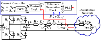
Figure 1: A single-phase grid-feeding VSI connected to distribution network.

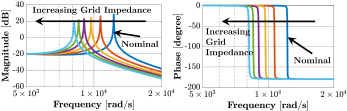
Figure 2: Bode plot of $\mathcal{G}_{inv}$ with varying grid impedance.

II Plant Model Description of Grid-Feeding VSI

The power circuit of a single-phase gfVSI connected to a distribution network at the point of common coupling (PCC) is shown in Fig. 1. The VSI is composed of a dc bus, $V_{dc}$, four switching devices, $S_{1},S_{2},S_{3},S_{4}$, and an $LCL$ filter with $L_{f}$, $L_{g}$ and $C_{f}$ as filter inductors and capacitor respectively with $R_{f}$ and $R_{g}$ as parasitic resistances of filter inductors. The distribution network is represented by the Thevenin equivalent voltage source, $v_{Th}$, in series with the Thevenin equivalent impedance $Z_{Th}:=R_{Th}+j\omega_{o}L_{Th}$ where $\omega_{o}$ (in rad/sec) is the nominal frequency of the distribution network. The VSI operates in $P$-$Q$ control mode by employing a current control strategy to regulate its output real and reactive power while being supported by a stable voltage and frequency source such as the grid, hence called grid-feeding VSI. The controller uses sinusoidal PWM switching technique to generate the switching signals. The dynamics of the VSI are described as:

$$L_{f}\frac{d\langle i_{L}\rangle}{dt}+R_{f}\langle i_{L}\rangle =\langle v_{inv}\rangle-\langle v_{C}\rangle,$$ (1)

$$L_{T}\frac{d\langle i_{inv}\rangle}{dt}+R_{T}\langle i_{inv}\rangle =\langle v_{C}\rangle-\langle v_{Th}\rangle,$$ (2)

$$C_{f}\frac{d\langle v_{C}\rangle}{dt} =\langle i_{L}\rangle-\langle i_{inv}\rangle,$$ (3)

where $\langle.\rangle$ signifies the average values of the corresponding variable over one switching cycle ($T_{s}$) [5]. Laplace transformation and algebraic manipulation with (1), (2) and (3) result:

$$I_{inv}(s) =\mathcal{G}_{inv}(s)V_{inv}(s)-\mathcal{G}_{Th}(s)V_{Th}(s),$$ (4)

where, $\mathcal{G}_{inv}(s)$ and $\mathcal{G}_{Th}(s)$ are transfer functions parameterized by $L_{f}$, $R_{f}$, $C_{f}$, $L_{T}:=L_{g}+L_{Th}$ and $R_{T}:=R_{g}+R_{Th}$.

III Impacts of Network on Plant Model Dynamics

As observed in (4), distribution network has impacts on the open-loop plant dynamics of a gfVSI. Firstly, both $\mathcal{G}_{inv}(s)$ and $\mathcal{G}_{Th}(s)$ consist of $L_{T}$ and $R_{T}$ (in turn consists of $L_{Th}$ and $R_{Th}$) as parameters that introduce uncertainties in the plant model. Secondly, $V_{Th}(s)$, imposed by the network, is acting as an exogenous disturbance signal to the plant. Where the latter one is a classical disturbance rejection problem, the severity of the former one questions the robust performance and needs to be discussed elaborately which is presented next.

III-A Effect of Thevenin Equivalent Grid Impedance Parameters

The resonant frequency of the $LCL$ circuit in Fig. 1, neglecting resistive elements of the circuit, is given as:

$$f_{res}=\dfrac{1}{2\pi}\sqrt{\dfrac{L_{f}+L_{T}}{L_{f}L_{T}C_{f}}}~{}(\text{in}~{}\text{Hz}).$$ (5)

The presence of parasitic resistances can provide passive damping to the resonance phenomenon, however minimal. Therefore, it is recommended to keep the pass-band of the current controller smaller than the resonant frequency, pre-determined based on the designed $L_{f}$, $L_{g}$ and $C_{f}$, in order to avoid instability due to resonance phenomenon. However, it is observed that the resultant resonant frequency is sensitive to grid parameters, especially grid inductance ($L_{Th}$). In case of a stiff grid with small $L_{Th}$, provided a properly designed filter, it can be ensured, to some extent, that the resultant resonant frequency is larger than the bandwidth of the controller. However, this issue is more severe in case of a weak grid system associated with large $L_{Th}$. For a sufficiently weak grid, the resultant resonance frequency may decrease and the corresponding resonance peak may enter the pass-band of the current controller as illustrated in Fig. 2. This uncertainty in grid impedance introduces difficulties in controller design [17]. In severe most situation, e.g. weak grid conditions, due to low-power transformers and long power lines in rural areas, this in turn results in instability of the gfVSIs as evidenced in [18].

III-B Modeling of Uncertain Grid Impedance

A systematic design of grid impedance variation for leveraging the gfVSI control is elaborated in this section. The open-loop plant model for the controller, as given in (1), (2), (3), of the circuit configuration in Fig. 1 is shown in Fig. 3 (inside the blue box). Clearly, variations in grid impedance (i.e. $R_{Th}$ and $L_{Th}$) results in real-parametric uncertainties in the parameters, $R_{T}$, $L_{T}$, of the transfer function (highlighted in red) in Fig. 3. The short-circuit ratio (SCR) is often used to characterize the grid stiffness/weakness and it comes handy in determining the equivalent impedance of the grid at the PCC [17]. It is mathematically defined as $(V_{PCC}^{Nom})^{2}/\big{[}S_{B}\sqrt{(\omega_{o}L_{g})^{2}+R_{g}^{2}}\big{]}$, where, $V_{PCC}^{Nom}$ is the nominal RMS voltage at PCC, and $S_{B}$ is the rated apparent power of the gfVSI. Usually the grid at PCC is considered as weak when the SCR is less than $3$. In this work, with a pre-specified SCR ($<3$) and given $X/R$ ratio of grid, the nominal grid impedance parameter are determined, denoted as $L^{N}_{Th}$ and $R^{N}_{Th}$. By considering $\pm 100\%$ variations over nominal values, it is assumed that $L_{Th}\in[\underline{L}_{Th},\bar{L}_{Th}]$ and $R_{Th}\in[\underline{R}_{Th},\bar{R}_{Th}]$. It is to be noted that very stiff to extremely weak grid conditions are considered by designing the grid impedance parameters in this way. As a result,

$$L_{T}:=L_{T}^{N}+w_{L}\delta_{L},~{}R_{T}:=R_{T}^{N}+w_{R}\delta_{R},$$ (6)

where, $\delta_{L}\in[-1,1]$, $\delta_{R}\in[-1,1]$, $L_{T}^{N}=L_{g}+\frac{1}{2}[\bar{L}_{Th}+\underline{L}_{Th}]$, $R_{T}^{N}=R_{g}+\frac{1}{2}[\bar{R}_{Th}+\underline{R}_{Th}]$, $w_{L}=\frac{1}{2}[\bar{L}_{Th}-\underline{L}_{Th}]$ and $w_{R}=\frac{1}{2}[\bar{R}_{Th}-\underline{R}_{Th}]$. This is the classical real parametric uncertainty modeling, quite commonly found in robust control theory. However, in synthesizing the controller with defined uncertainties in $1/(L_{T}s+R_{T})$, this representation is quite difficult to handle. Linear fractional transformation (LFT) approach can be utilized to convert the model into an upper LFT, given by $F_{U}(\mathbf{M},\mathbf{\Delta})$ as follows[20] :

$$\underbrace{\left[\begin{array}[]{c|c}\mathbf{M_{11}}&\mathbf{M_{12}}\\ \hline\cr\mathbf{M_{21}}&\mathbf{M_{22}}\end{array}\right]}_{\mathbf{M}}=\dfrac{1}{sL_{T}^{N}+R_{T}^{N}}\left[\begin{array}[]{c | c}\begin{array}[]{c c}-sw_{L}&-w_{R}\\ -sw_{L}&-w_{R}\end{array}&\begin{array}[]{c c}1\\ 1\end{array}\\ \hline\cr\begin{array}[]{c c}-sw_{L}&-w_{R}\end{array}&1\end{array}\right],$$

$$~{}s.t.~{}\dfrac{1}{sL_{T}+R_{T}}=\mathbf{M_{22}}+\mathbf{M_{21}\Delta(I-M_{11}\Delta)^{-1}M_{12}},$$

where, $\mathbf{\Delta}=diag(\delta_{L},\delta_{R})$.

IV Proposed $\mathcal{H}_{\infty}$-Based Solution

IV-A Objectives and Operation of the Control System

A $P$-$Q$ controlled gfVSI operates to inject a pre-specified reference active power, $P_{ref}$, and reactive power, $Q_{ref}$, (defined locally/centrally) into the network by employing a current control strategy [1]. An outer ‘Reference Generation Block’ (as shown in Fig. 1) eventually generates the $i_{ref}$ signal using its $P$-$Q$ set-points and output signals from phase-locked loop (PLL). The expression of $i_{ref}$ is given by

$$i_{ref}(t)=\sqrt{2}\frac{\sqrt{P_{ref}^{2}+Q_{ref}^{2}}}{\bar{V}}\sin\bigg{(}{\tilde{\theta}-\arctan{\frac{Q_{ref}}{P_{ref}}}}\bigg{)}.$$ (7)

A PLL operates with its grid-synchronization technique and generates signals, $\bar{V}$, $\tilde{\theta}$, containing the RMS value and synchronized phase information of $v_{PCC}$ respectively. In this work, a 1-$\phi$ second order generalized integrator-based synchronous reference frame PLL (SOGI-SRF-PLL) is used [21]. The generated $i_{ref}$ along with the measured $i_{inv}$ are the inputs to the ‘Control Logic’ block as shown in Fig. 1. The objective here is to design a feedback control law through controller, $\mathcal{C}_{\mathcal{H}_{\infty}}(s)$ as shown in Fig. 3, which generates a control signal, $v_{inv}$, such that, i) $i_{inv}$ tracks $i_{ref}$ with minimum tracking error, ii) effects of $v_{Th}$ on $i_{inv}$ is largely attenuated, iii) $v_{inv}$ satisfies the bandwidth limitations. Moreover, all aforementioned objectives need to be satisfied with model uncertainties. In other words, it is necessary to provide the controller with enough robustness to deal with uncertainties caused by the distribution network. These objectives are derived from acceptable standards on power quality, e.g. IEEE Std 519[22].

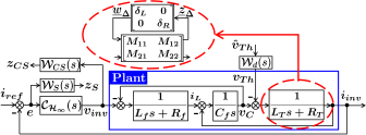
Figure 3: Proposed $\mathcal{H}_{\infty}$-based robust current controller synthesis.

IV-B Design Procedure of the $\mathcal{H}_{\infty}$-based Controller

$\mathcal{H}_{\infty}$-based controller design provides a framework for addressing multiple objectives. Here, the design is based on the system structure illustrated in Fig. 3 where user-defined weighting transfer functions, $\mathcal{W}_{{S}}(s)$, $\mathcal{W}_{CS}(s)$, $\mathcal{W}_{d}(s)$, are selected based on the aforementioned objectives. The guidelines for designing the weighting functions are provided below.

IV-B1 Selection of $\mathcal{W}_{S}(s)$

To shape the sensitivity transfer function, the weighting function, $\mathcal{W}_{S}(s)$, is introduced so that

• the tracking error, $e$, at fundamental frequency is low,

• the $LCL$ filter resonance of the VSI is actively damped.

$\mathcal{W}_{S}(s)$ is modeled to have peaks around $\omega_{o}$ and $LCL$ resonant frequency, $\omega_{r}$, with $2^{nd}$ order roll-off, $k_{S,1}(s)$ and formed as

$$\mathcal{W}_{S}(s)=k_{S,1}(s)\dfrac{s^{2}+2k_{S,2}\zeta\omega_{o}s+\omega_{o}^{2}}{s^{2}+2\zeta\omega_{o}s+\omega_{o}^{2}}\dfrac{s^{2}+2k_{S,3}\zeta\omega_{r}s+\omega_{r}^{2}}{s^{2}+2\zeta\omega_{r}s+\omega_{r}^{2}},$$

where, $k_{S,2}$ and $k_{S,3}$ are selected to exhibit peaks and $\zeta$ takes care of the off-nominal frequency around the nominal values.

IV-B2 Selection of $\mathcal{W}_{CS}(s)$

$\mathcal{W}_{CS}(s)$ is designed to suppress high-frequency control effort to shape the performance of $v_{inv}$. Hence, it is designed as a high-pass filter with cut-off frequency at switching frequency and is ascribed the form:

$$\mathcal{W}_{CS}(s)=k_{CS}\dfrac{s+k_{CS,1}\omega_{o}}{s+k_{CS,2}\omega_{o}},~{}\text{where}~{}k_{CS,1}<<k_{CS,2}.$$

IV-B3 Selection of $\mathcal{W}_{d}(s)$

$\mathcal{W}_{d}(s)$ emphasizes the expected disturbances at fundamental and harmonic frequencies imposed by $v_{Th}$ and emphasized by exogenous signal $\hat{v}_{Th}$. It is based on the assumption that the network voltage comprises fundamental and considerable amount of $3^{rd}$, $5^{th}$, $7^{th}$ harmonics [22]. Hence, it is designed by a low-pass filter, $k_{d}(s)$, with peaks at selected frequencies and is ascribed the form:

$$\mathcal{W}_{d}(s)=k_{d}(s)\prod_{h=1,3,5,7}\dfrac{s^{2}+2k_{d,h}\zeta h\omega_{o}s+h^{2}\omega_{o}^{2}}{s^{2}+2\zeta h\omega_{o}s+h^{2}\omega_{o}^{2}},$$

where, the values of $k_{d,h}$ are selected based on the voltage THD standards recommended in IEEE Std-519 [22].

IV-C Problem Formulation and Resulting Optimal Controller

The Bode plots of the selected weighting transfer functions in this work are shown in Fig. 4LABEL:sub@fig:weight. The $\mathcal{H}_{\infty}$-based optimal problem is formulated and solved to generate a feedback control law with resulting controller, $\mathcal{C}_{\mathcal{H}_{\infty}}(s)$, stated as:

$$V_{inv}(s)=\mathcal{C}_{\mathcal{H}_{\infty}}(s)[I_{ref}(s)-I_{inv}(s)].$$ (8)

As a result, the closed loop system equation for the VSI can be found by combining (4) and (8) and can be written as

$$I_{inv}(s)=\mathcal{G}(s)I_{ref}(s)-\mathcal{Y}(s)V_{Th}(s),$$ (9)

where,

$$\mathcal{G}(s)=\dfrac{\mathcal{G}_{inv}(s)\mathcal{C}_{\mathcal{H}_{\infty}}(s)}{1+\mathcal{G}_{inv}(s)\mathcal{C}_{\mathcal{H}_{\infty}}(s)},~{}\mathcal{Y}(s)=\dfrac{\mathcal{G}_{Th}(s)}{1+\mathcal{G}_{inv}(s)\mathcal{C}_{\mathcal{H}_{\infty}}(s)}.$$

Remark.

It is equivalent to state that the optimal controller is required to be designed satisfying the following conditions: $\mathcal{G}(s)|_{s=j\omega_{o}}\approx 1\angle 0^{o}$ and $\mathcal{Y}(s)|_{s=jh\omega_{o}}<<1$ for $h=1,3,5,7$.

The control system of Fig. 3 can be realized as a generalized control configuration as shown in Fig. 4LABEL:sub@fig:control2[20]. It has a generalized MIMO plant, $\mathcal{P}(s)$, containing all nominal models, $\mathbf{M}$, $\mathcal{W}_{S}(s)$, $\mathcal{W}_{CS}(s)$ and $\mathcal{W}_{d}(s)$ with exogenous input signal ${w}:=\begin{bmatrix}\underline{w}_{\Delta}&i_{ref}&\hat{v}_{Th}&{v}_{inv}\end{bmatrix}^{\top}$ and output signals ${z}:=\begin{bmatrix}\underline{z}_{\Delta}&z_{S}&z_{CS}&e\end{bmatrix}^{\top}$. The controller, $\mathcal{C}_{\mathcal{H}_{\infty}}(s)$ has input feedback signal, $e$, and output control signal, ${v}_{inv}$. The uncertainty function, $\mathbf{\Delta}$, with input $\underline{z}_{\Delta}$ and output $\underline{w}_{\Delta}$ is represented using upper LFT [20]. The goal is to synthesize the stabilizing controller that satisfies the following:

$$||T_{w\rightarrow z}||_{\infty}<1.$$ (10)

By means of hinfsyn command of MATLAB robust control toolbox, the synthesis of optimal controller is achieved. Usually $\mathcal{H}_{\infty}$-control algorithms produce controllers of higher order and model reduction becomes essential to design a low order implementable controller. It is achieved by using balanced truncation method removing modes faster than the switching frequency. The resulting controller, $\mathcal{C}_{\mathcal{H}_{\infty}}(s)$, is of the order of 11 which is higher than that of conventional PR controller with harmonic compensators only by 3. Fig. 5LABEL:sub@fig:GYmag and 5LABEL:sub@fig:GYphase corroborate the accomplishment of the objectives by the resulting optimal controller with $||T_{w\rightarrow z}||_{\infty}=0.63$. Robust stability is verified by robstab command of MATLAB.

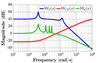
(a)

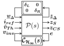
(b)

Figure 4: (a) Bode plots of magnitudes of selected weighting transfer functions, (b) generalized control configuration of Fig. 3.

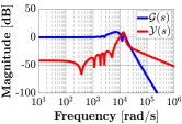
(a)

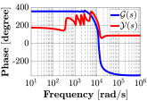
(b)

Figure 5: Bode plots, (a) magnitudes of $\mathcal{G}(s)$, $\mathcal{Y}(s)$, (b) phase of $\mathcal{G}(s)$, $\mathcal{Y}(s)$.

V Validation and Results

The computational footprint of the proposed $\mathcal{H}_{\infty}$-based controller, an essential check for validating the performance while implemented in a real low-cost micro-controller board, is discussed here with a brief description of the test system.

V-A Controller Hardware-in-the-loop Setup Description

Controller hardware-in-the-loop (CHIL)-based simulation studies are conducted on OPAL-RT real-time simulator. North American low voltage distribution feeder from CIGRE Task Force C6.04.02, affiliated with CIGRE Study Committee C6 is emulated inside the OPAL-RT along with the power circuit of a gfVSI, connected at $\text{Bus}_{\text{12}}$ with parameters tabulated in Table I. Ratings of distribution transformer, loads at each bus and line parameters are provided in [23]. The test system is modified by including sufficient amount of non-linear loads at various buses while respecting the recommended limits of THD mentioned in [22]. The proposed resulting $\mathcal{H}_{\infty}$-based controller is realized on a low-cost Texas-Instruments TMS28379D Delfino controller board as shown in Fig. 6.

TABLE I: GRID AND GRID-FEEDING VSI PARAMETERS UNDER STUDY

VSI Parameter	Value
Ratings	$240$ V (RMS), $60$ Hz, $11$ kVA, $0.95$ pf
VSI Parameters	$V_{dc}$ = $500$ V, $f_{Sw}$ = $20$ kHz
$LCL$ Filter Parameters	$L_{f}$ = $2$ mH, $L_{g}$ = $400$ $\mu$H, $C_{f}$ = $20~{}\mu$F
Grid Parameter	Value
Grid Impedance	$L_{Th}\in[0,0.53]$ mH, $R_{Th}\in[0,0.05]$ $\Omega$

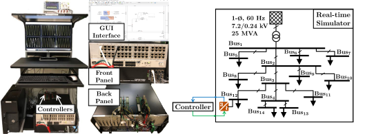
Figure 6: OPAL-RT based hardware-in-the-loop simulation platform with CIGRE test system and Texas Instruments Delfino TMS320F28379D controller board.

V-B CHIL-based Experimental Result

Two test cases are examined by emulating a sequence of events in the OPAL-RT platform. Test cases are enlisted as:

• $\mathtt{CASE}$-$\mathtt{1}$: The VSI is initially in no-load condition. At $t=50.03~{}s$, there is a transition from no-load to full-load and stays until $t=50.2~{}s$. $20$% under-voltage (of nominal) occurs at $t=50.12~{}s$ and stays until $t=50.28~{}s$ when voltage revives to nominal value. During this interval, VSI is overloaded by $150$% from $t=50.2~{}s$. At $t=50.28~{}s$, the VSI is switched to rated load condition until $t=50.36~{}s$ when it switches over to no load condition.

• $\mathtt{CASE}$-$\mathtt{2}$: The VSI is operating in rated loading with a sudden jump of equivalent grid inductance from $0$ mH to $0.53$ mH at $t=17.53~{}s$ while maintaining same loading.

The results for $\mathtt{CASE}$-$\mathtt{1}$ are shown in Fig. 7. It is clearly observed that the output current waveforms of VSI, $i_{inv}$, is following $i_{ref}$ with minimal tracking error as shown in Fig. 7LABEL:sub@fig:result1. The current and power outputs are maintained during the sudden changes of $v_{PCC}$ as illustrated in Fig. 7LABEL:sub@fig:result2. Thus, the performance of the proposed controller of reference tracking and disturbance rejection are validated in this case studies. The results for $\mathtt{CASE}$-$\mathtt{2}$ are shown in Fig. 8LABEL:sub@fig:result3 and Fig. 8LABEL:sub@fig:result4. It is observed that the performance of the proposed current controller is sufficiently robust to a substantial amount of variations in equivalent grid impedance and that validates the robust performance of the proposed controller.

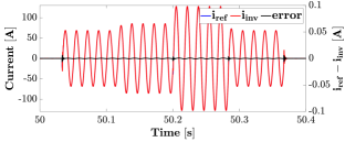
(a)

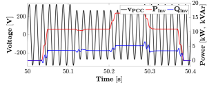
(b)

Figure 7: CHIL simulation results for $\mathtt{CASE}$-$\mathtt{1}$, (a) output current and reference waveform with tracking error, (b) power output and voltage waveform at PCC.

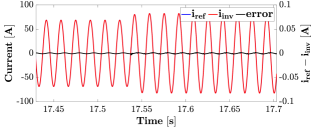
(a)

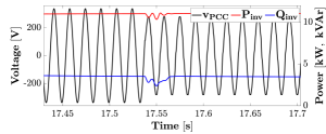
(b)

Figure 8: CHIL simulation results for $\mathtt{CASE}$-$\mathtt{2}$, (a) output current and reference waveform with tracking error, (b) power output and voltage waveform at PCC.

V-C Performance Comparison

For the purpose of performance comparison, PR-based current controller with PCC voltage feed-forward is considered for the CHIL simulation. Reference [5] provides an elaborated guidelines for designing the current controller with sufficient gain and phase margins in order to possess a fair comparative study. The current loop with PR controller is designed to have PM $\geq 45^{\circ}$ and GM $\geq 40$ dB with bandwidth of $1.5$ kHz. Similar to $\mathtt{CASE}$-$\mathtt{1}$ and $\mathtt{CASE}$-$\mathtt{2}$, $\mathtt{CASE}$-$\mathtt{3}$ study is conducted for comparison study of proposed $\mathcal{H}_{\infty}$-based controller with PR controller in this work. The case study is as follows:

• $\mathtt{CASE}$-$\mathtt{3}$: The VSI is operating at rated loading with minimal grid impedance (stiff grid) until $t=17.53~{}s$ when there is a sudden jump of grid inductance from $0.1$ mH to $0.53$ mH (weak grid). Moreover, at $t=17.62~{}s$ VSI jumps to $150\%$ loading condition with weak grid.

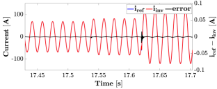
(a)

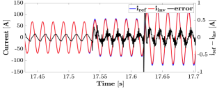
(b)

Figure 9: CHIL simulation results for $\mathtt{CASE}$-$\mathtt{3}$ with output current and reference waveform, tracking error, (a) $\mathcal{H}_{\infty}$-based controller, (b) PR controller.

The results for $\mathtt{CASE}$-$\mathtt{3}$ are shown in Fig. 9. It is observed that the output current of VSI, $i_{inv}$, is following $i_{ref}$ with large tracking error in PR controller once the grid stiffness weakens as shown in Fig. 7LABEL:sub@fig:result5 and Fig. 7LABEL:sub@fig:result7 respectively. The results substantiate the fact that the proposed $\mathcal{H}_{\infty}$-based controller exhibits superior robustness in performance than the PR controller at the cost of increasing the order of controller only by $3$ and no additional sensor requirements.

VI Conclusions

This article demonstrates the design and implementation of a robust current controller for single-phase gfVSI. The uncertainty in grid impedance is modeled explicitly to leverage the robustness in performance of the controller. $\mathcal{H}_{\infty}$-based controller design is followed and the required objectives for the optimal controller are discussed which leads to the final optimal controller. OPAL-RT based CHIL studies are conducted to verify the viability of the resulting controller. Moreover performance with classical PR based controller are compared to highlights the superiority of the proposed controller.

References

- [1] J. P. Lopes, C. Moreira, and A. Madureira, “Defining control strategies for microgrids islanded operation,” IEEE Transactions on power systems, vol. 21, no. 2, pp. 916–924, 2006.
- [2] J. Lettl, J. Bauer, and L. Linhart, “Comparison of different filter types for grid connected inverter,” PIERS Proceedings, Marrakesh, Morocco, 2011.
- [3] K. Arulkumar, P. Manojbharath, S. Meikandasivam, and D. Vijayakumar, “Robust control design of grid power converters in improving power quality,” in 2015 International Conference on Technological Advancements in Power and Energy (TAP Energy). IEEE, 2015, pp. 460–465.
- [4] M. Ebrahimi, S. A. Khajehoddin, and M. Karimi-Ghartemani, “Fast and robust single-phase current controller for smart inverter applications,” IEEE transactions on power electronics, vol. 31, no. 5, pp. 3968–3976, 2015.
- [5] A. Yazdani and R. Iravani, Voltage-sourced converters in power systems. Wiley Online Library, 2010, vol. 34.
- [6] C. Xie, X. Zhao, K. Li, J. Zou, and J. M. Guerrero, “A new tuning method of multiresonant current controllers for grid-connected voltage source converters,” IEEE Journal of Emerging and Selected Topics in Power Electronics, vol. 7, no. 1, pp. 458–466, 2018.
- [7] A. Timbus, M. Liserre, R. Teodorescu, P. Rodriguez, and F. Blaabjerg, “Evaluation of current controllers for distributed power generation systems,” IEEE Transactions on power electronics, vol. 24, no. 3, pp. 654–664, 2009.
- [8] H. M. Kojabadi, B. Yu, I. A. Gadoura, L. Chang, and M. Ghribi, “A novel dsp-based current-controlled pwm strategy for single phase grid connected inverters,” IEEE transactions on power electronics, vol. 21, no. 4, pp. 985–993, 2006.
- [9] M. Su, B. Cheng, Y. Sun, Z. Tang, B. Guo, Y. Yang, F. Blaabjerg, and H. Wang, “Single-sensor control of lcl-filtered grid-connected inverters,” Ieee Access, vol. 7, pp. 38 481–38 494, 2019.
- [10] M. Huang, Q. Tan, H. Li, and W. Wu, “Improved sliding mode control method of single-phase lcl filtered vsi,” in 2018 9th IEEE International Symposium on Power Electronics for Distributed Generation Systems (PEDG). IEEE, 2018, pp. 1–5.
- [11] J. N. da Silva, A. J. Sguarezi Filho, D. A. Fernandes, A. P. Tahim, E. R. da Silva, and F. F. Costa, “A discrete repetitive current controller for single-phase grid-connected inverters,” in 2017 Brazilian Power Electronics Conference (COBEP). IEEE, 2017, pp. 1–6.
- [12] Leming Zhou, An Luo, Y. Chen, Xiaoping Zhou, and Zhiyong Chen, “A novel two degrees of freedom grid current regulation for single-phase lcl-type photovoltaic grid-connected inverter,” in 2016 IEEE 8th International Power Electronics and Motion Control Conference (IPEMC-ECCE Asia), May 2016, pp. 1596–1600.
- [13] J. Xu, S. Xie, B. Zhang, and Q. Qian, “Robust grid current control with impedance-phase shaping forlcl-filtered inverters in weak and distorted grid,” IEEE Transactions on Power Electronics, vol. 33, no. 12, pp. 10 240–10 250, 2018.
- [14] W. Wu, Y. He, and F. Blaabjerg, “An llcl power filter for single-phase grid-tied inverter,” IEEE Transactions on Power Electronics, vol. 27, no. 2, pp. 782–789, 2011.
- [15] I. J. Gabe, V. F. Montagner, and H. Pinheiro, “Design and implementation of a robust current controller for vsi connected to the grid through an lcl filter,” IEEE Transactions on Power Electronics, vol. 24, no. 6, pp. 1444–1452, 2009.
- [16] T. Hornik and Q.-C. Zhong, “A current-control strategy for voltage-source inverters in microgrids based on h and repetitive control,” IEEE Transactions on Power Electronics, vol. 26, no. 3, pp. 943–952, 2010.
- [17] M. S. Sadabadi, A. Haddadi, H. Karimi, and A. Karimi, “A robust active damping control strategy for an -based grid-connected dg unit,” IEEE Transactions on Industrial Electronics, vol. 64, no. 10, pp. 8055–8065, 2017.
- [18] Y. Han, Z. Li, P. Yang, C. Wang, L. Xu, and J. M. Guerrero, “Analysis and design of improved weighted average current control strategy for lcl-type grid-connected inverters,” IEEE Transactions on Energy Conversion, vol. 32, no. 3, pp. 941–952, 2017.
- [19] J. Wang, I. Tyuryukanov, and A. Monti, “Design of a novel robust current controller for grid-connected inverter against grid impedance variations,” International Journal of Electrical Power & Energy Systems, vol. 110, pp. 454–466, 2019.
- [20] S. Skogestad and I. Postlethwaite, Multivariable feedback control: analysis and design. Wiley New York, 2007, vol. 2.
- [21] M. Ciobotaru, R. Teodorescu, and F. Blaabjerg, “A new single-phase pll structure based on second order generalized integrator,” in 2006 37th IEEE Power Electronics Specialists Conference. IEEE, 2006, pp. 1–6.
- [22] “Ieee recommended practice and requirements for harmonic control in electric power systems,” IEEE Std 519-2014 (Revision of IEEE Std 519-1992), pp. 1–29, June 2014.
- [23] K. Strunz, R. H. Fletcher, R. Campbell, and F. Gao, “Developing benchmark models for low-voltage distribution feeders,” in 2009 IEEE Power Energy Society General Meeting, July 2009, pp. 1–3.