The Coupling/Minorization/Drift Approach to

Markov Chain Convergence Rates

by (in alphabetical order)

Yu Hang Jiang, Tong Liu, Zhiya Lou, Jeffrey S. Rosenthal, Shanshan Shangguan, Fei Wang, and Zixuan Wu

Department of Statistical Sciences, University of Toronto

(August 18, 2020; last revised )

Abstract: This review paper provides an introduction of Markov chains and their convergence rates – an important and interesting mathematical topic which also has important applications for very widely used Markov chain Monte Carlo (MCMC) algorithm. We first discuss eigenvalue analysis for Markov chains on finite state spaces. Then, using the coupling construction, we prove two quantitative bounds based on minorization condition and drift conditions, and provide descriptive and intuitive examples to showcase how these theorems can be implemented in practice. This paper is meant to provide a general overview of the subject and spark interest in new Markov chain research areas.

1 Introduction

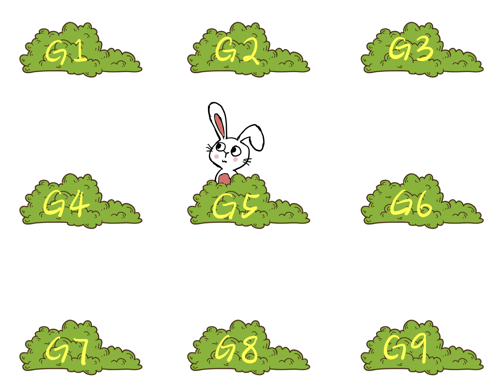
Figure 1: The bunny example

Imagine there is a $3\times 3$ grid of bushes, labeled $G_{1},G_{2},...,G_{9}$, from top to bottom and left to right (Figure 1). There is a fluffy little bunny hiding in the middle bush, starving and ready to munch on some grass around it. Assume the bunny never gets full and the grass is never depleted. Once each minute, the bunny jumps from its current bush to one of the nearest other bushes (up, down, left, or right, not diagonal) or stays at its current location, each with equal probability. We can then ask about longer-term probabilities. For example, if the bunny starts at G5, the probability of jumping to $G_{7}$ after two steps is:

$${\rm Prob}_{G5}(\mathrm{at}\ G_{7}\ \mathrm{after\ two\ steps}) ={\rm Prob}(G_{5}\to G_{4}\to G_{7})+{\rm Prob}(G_{5}\to G_{8}\to G_{7})$$

$$=\frac{1}{5}\times\frac{1}{4}+\frac{1}{5}\times\frac{1}{4}=\frac{1}{10}\,.$$

But what happens to the probabilities after three steps? ten steps? more?

This paper investigates the convergence of such probabilities as the number of steps gets larger. As we will discuss later, such bounds are not only an interesting topic in their own right, they are also very important for reliably using Markov chain Monte Carlo (MCMC) computer algorithms [3, 2, 1] which are very widely applied to numerous problems in statistics, finance, computer science, physics, combinatorics, and more. After reviewing the standard eigenvalue approach in Section 3, we will concentrate on the use of “coupling”, and specifically on the use of “minorization” (Section 4) and “drift” (Section 6) conditions. We note that coupling is a very broad topic with many different variations and applications (see e.g. [9]), and has even inspired its own algorithms (such as “coupling from the past”). And, there are many other methods of bounding convergence of Markov chains, including continuous-time limits, different metrics, path coupling, non-Markovian couplings, spectral analysis, operator theory, and more, as well as numerous other related topics, which we are not able to cover here.

2 Markov Chains

The above bunny model is an example of a Markov chain (in discrete time and space). In general, a Markov chain is specified by three ingredients:

1. A state space $\mathcal{X}$, which is a collection of all of the states the Markov chain might be at. In the bunny example, $\mathcal{X}=\{G_{1},G_{2},...,G_{9}\}$.

2. An initial distribution (probability measure) $\mu_{0}(\cdot)$, where $\mu_{0}(A)$ is the probability of starting within $A\subset\mathcal{X}$ at time 0. In the bunny example, $\mu_{0}(G_{5})=1$, and $\mu_{0}(G_{i})=0\ \forall i\neq 5$.

3. A collection of transition probability distributions $P(x,\cdot)$ on $\mathcal{X}$ for each state $x\in\mathcal{X}$. The distribution $P(x,\cdot)$ represents the probabilities of the Markov chain going from $x$ to the next state after one unit of time. In a discrete state space like the bunny example, the transition probabilities can be simply written as $P=\{p_{ij}\}_{i,j\in\mathcal{X}}$, where $p_{ij}$ is the probability of jumping to $j$ from $i$. Indeed, in the bunny example:

For example, in the second row, $p_{21}=p_{22}=p_{23}=p_{25}=\frac{1}{4}$ because from $G_{2}$, the probabilities of jumping to each of $G_{1}$, $G_{2}$, $G_{3}$, or $G_{5}$ are each $\frac{1}{4}$.

We write $\mu_{n}(i)$ for the probability that the Markov chain is at state $i$ after $n$ steps. Given the initial distribution $\mu_{0}$ and transition probabilities $P(x,\cdot)$, we can compute $\mu_{n}$ inductively by

$$\mu_{n}(A):=\int_{x\in\mathcal{X}}P(x,A)\ \mu_{n-1}(dx)\,,\qquad n\geq 1\,.$$

On a discrete space, this formula reduces to $\mu_{n}(j)=\sum_{i\in\mathcal{X}}p_{ij}\,\mu_{n-1}(i)$. In matrix form, regarding the $\mu_{n}$ as row-vectors, this means $\mu_{n}=\mu_{n-1}\,P$. It follows by induction that $\mu_{n}=\mu_{0}\,P^{n}$, where $P^{n}$ is the $n$’th matrix power of $P$, also called the $n$-step transition matrix. Here $(P^{n})_{ij}$ is the probability of jumping to $j$ from $i$ in $n$ steps. Indeed, if we take $\mu_{0}=(0,0,\dots,1,\dots,0)$, so $\mu_{0}(i)=1$ with $\mu_{0}(j)=0$ for all $j\not=i$, then $\mu_{n}(j)=\sum_{r=0}\mu_{0}(r)(P^{n})_{rj}=(P^{n})_{ij}$. This makes sense since if we start at $i$, then $\mu_{n}(j)$ is the probability of moving from $i$ to $j$ in $n$ steps.

One main question in Markov chain analysis is whether the probabilities $\mu_{n}$ will converge to a certain distribution, i.e. whether $\pi:=\lim_{n\to\infty}\mu_{n}$ exists. If it does, then letting $n\to\infty$ in the relation $\mu_{n+1}=\mu_{n}P$ indicates that $\pi$ must be stationary, i.e. $\pi=\pi P$. On a finite state space, this means that $\pi$ is a left eigenvector of the matrix $P$ with corresponding eigenvalue 1.

In the bunny example, by solving the system of linear equations given by $\pi P=\pi$, the stationary probability distribution can be computed to be the following vector:

$$\pi\ =\ \bigg{(}\frac{1}{11},\frac{4}{33},\frac{1}{11},\frac{4}{33},\frac{5}{33},\frac{4}{33},\frac{1}{11},\frac{4}{33},\frac{1}{11}\bigg{)}\,.$$

In fact, the bunny example satisfies general theoretical properties called irreducibility and aperiodicity, which guarantee that the stationary distribution $\pi$ is unique, and that $\mu_{n}$ converges to $\pi$ as $n\to\infty$ (see e.g. [8]). However, in this paper we shall focus on quantitative convergence rates, i.e. how large $n$ has to be to make $\mu_{n}$ sufficiently close to $\pi$.

3 Eigenvalue Analysis on Finite State Spaces

When the state space is finite and small, it is sometimes possible to obtain a quantitative bounds on the convergence rate through direct matrix analysis (e.g. [6]). We require eigenvalues $\lambda_{i}$ and left-eigenvectors $v_{i}$ such that $v_{i}P=\lambda_{i}v_{i}$. For example, for the above bunny process, we compute (numerically, for simplicity) that the eigenvalues and left-eigenvectors are:

$$(\lambda_{0},\lambda_{1},\lambda_{2},\lambda_{3},\lambda_{4},\lambda_{5},\lambda_{6},\lambda_{7},\lambda_{8})=(1,0.702,0.702,-0.467,0.333,0.25,0.25,0.119,0.119)$$

$$\begin{pmatrix}v_{0}\\ v_{1}\\ v_{2}\\ v_{3}\\ v_{4}\\ v_{5}\\ v_{6}\\ v_{7}\\ v_{8}\\ \end{pmatrix}=\begin{pmatrix}0.091&0.121&0.091&0.121&0.152&0.121&0.091&0.121&0.091\\ 0.489&0.361&0&0.361&0&-0.361&0&-0.361&-0.489\\ 0.055&-0.318&-4.863&0.399&0&-0.399&4.863&0.318&-0.055\\ -0.224&0.358&-0.224&0.358&-0.537&0.358&-0.224&0.358&-0.224\\ 0.500&0&-0.500&0&0&0&-0.500&0&0.500\\ 0.002&-0.500&0.002&0.499&-0.007&0.499&0.002&-0.500&0.002\\ 0.256&-0.043&0.256&-0.043&-0.854&-0.043&0.256&-0.043&0.256\\ -0.436&0.394&0&0.394&0&-0.394&0&-0.394&0.436\\ 0.018&0.377&-0.425&-0.410&0&0.410&0.435&-0.377&-0.018\\ \end{pmatrix}\\$$

To be specific, assume that the bunny starts from the center bush $G_{5}$, so $\mu_{0}=(0,0,0,0,1,0,0,0,0)$. We can express this $\mu_{0}$ in terms of the above eigenvector basis as the linear combination:

$$\mu_{0}\ =\ v_{0}-0.4255v_{3}-0.7259v_{6}\,.$$

(Here $v_{0}=\pi$, corresponding to the eigenvalue $\lambda_{0}=1$.) Recalling that $\mu_{n}=\mu_{0}P^{n}$, and that $v_{i}P=\lambda_{i}\,v_{i}$ by definition, we compute that e.g.

$$\mu_{n}(G_{5})=(\lambda_{0})^{n}v_{0}(G_{5})-0.4255(\lambda_{3})^{n}v_{3}(G_{5})-0.7259(\lambda_{6})^{n}v_{6}(G_{5})$$

$$=\pi(G_{5})-0.4255(-0.4667)^{n}(-0.537)-0.7259(0.25)^{n}(-0.854)\,.$$

Since $|0.25|<|0.4667|$, and $|0.4255\cdot(-0.537)|+|0.7259\cdot(-0.854)|<0.85$, the triangle inequality implies that

$$|\mu_{n}(G_{5})-\pi(G_{5})|<0.85\,(0.4667)^{n}\,,\quad n\in{\mathbb{N}}\,.$$

This shows that $\mu_{n}(G_{5})\to\pi(G_{5})$, and gives a strong bound on the difference between them. For example, $|\mu_{n}(G_{5})-\pi(G_{5})|<0.01$ whenever $n\geq 6$, i.e. only 6 steps are required to make the bunny’s probability of being at $G_{5}$ within 0.01 of its limiting (stationary) probability. Other states besides $G_{5}$ can be handled similarly.

Unfortunately, such direct eigenvalue or spectral analysis becomes more and more challenging on larger and more complicated examples, especially on non-finite state spaces. So, we next introduce a different technique which, while less tight, is more widely applicable.

4 Coupling and Minorization Conditions

The idea of coupling is to create two different copies of a random object, and compare them. Coupling has a long history in probability theory, with many different applications and approaches (see e.g. [9]). A key idea is the coupling inequality. Suppose we have two random variables $X$ and $Y$, each with their own distribution. Then for any subset $A$, we can write

$$\big{|}{\rm Prob}(X\in A)-{\rm Prob}(Y\in A)\big{|}\\ \ =\ \big{|}{\rm Prob}(X\in A,\ X=Y)+{\rm Prob}(X\in A,\ X\not=Y)\\ -{\rm Prob}(Y\in A,\ X=Y)-{\rm Prob}(Y\in A,\ X\not=Y)\big{|}\,.$$

But here ${\rm Prob}(X\in A,\ X=Y)={\rm Prob}(Y\in A,\ X=Y)$, since they both refer to the same event, so those two terms cancel. Also, each of ${\rm Prob}(X\in A,\ X\not=Y)$ and ${\rm Prob}(Y\in A,\ X\not=Y)$ are between 0 and ${\rm Prob}(X\not=Y)$, so their difference must be $\leq{\rm Prob}(X\not=Y)$. Hence,

$$\big{|}{\rm Prob}(X\in A)-{\rm Prob}(Y\in A)\big{|}\ \leq\ {\rm Prob}(X\not=Y)\,.$$

Since this upper bound is uniform over subsets $A$, we can even take a supremum over $A$, to also bound the total variation distance:

$$\left\lVert\mathcal{L}(X)-\mathcal{L}(Y)\right\rVert_{TV}\ :=\ \sup_{A\subseteq\mathcal{X}}\big{|}{\rm Prob}(X\in A)-{\rm Prob}(Y\in A)\big{|}\ \leq\ {\rm Prob}(X\not=Y)\,.$$

That is, the total variation distance between the probability laws $\mathcal{L}(X)$ and $\mathcal{L}(Y)$ is bounded above by the probability that the random variables $X$ and $Y$ are not equal. To apply this fact to Markov chains, the following condition is very helpful.

Definition.

A Markov chain with state space $\mathcal{X}$ and transition probabilities $P$ satisfies a minorization condition if there exists a (measurable) subset $C\subseteq\mathcal{X}$, a probability measure $\nu$ on $\mathcal{X}$, a constant $\epsilon>0$, and a positive integer $n_{0}$, such that

$$P^{n_{0}}(x,\cdot)\geq\epsilon\nu(\cdot),\ x\in C\,.$$

We call such $C$ a small set. In particular, if $C=\mathcal{X}$ (the entire state space), then the Markov chain satisfies a uniform minorization condition, also referred to as Doeblin’s condition.

For a concrete example, suppose the state space is the half-line $\mathcal{X}=[0,\infty)$, with transition probabilities given by

$$P(x,dy)\ =\ \Big{(}e^{-2y}+\frac{1}{\sqrt{2\pi}(x+1)}e^{-\frac{y^{2}}{2(x+1)^{2}}}\Big{)}\,dy\,.$$ (1)

That is, from a state $x$, the chain moves to an equal mixture of an Exponential(2) distribution and a half-normal distribution with mean 0 and standard deviation $x+1$. In this case, $P(x,dy)\geq e^{-2y}\,dy$ for all $x$ (see Figure 2), so the chain satisfies a uniform minorization condition with $n_{0}=1$, $\nu(y)=2e^{-2y}$, and $\epsilon=\frac{1}{2}$.

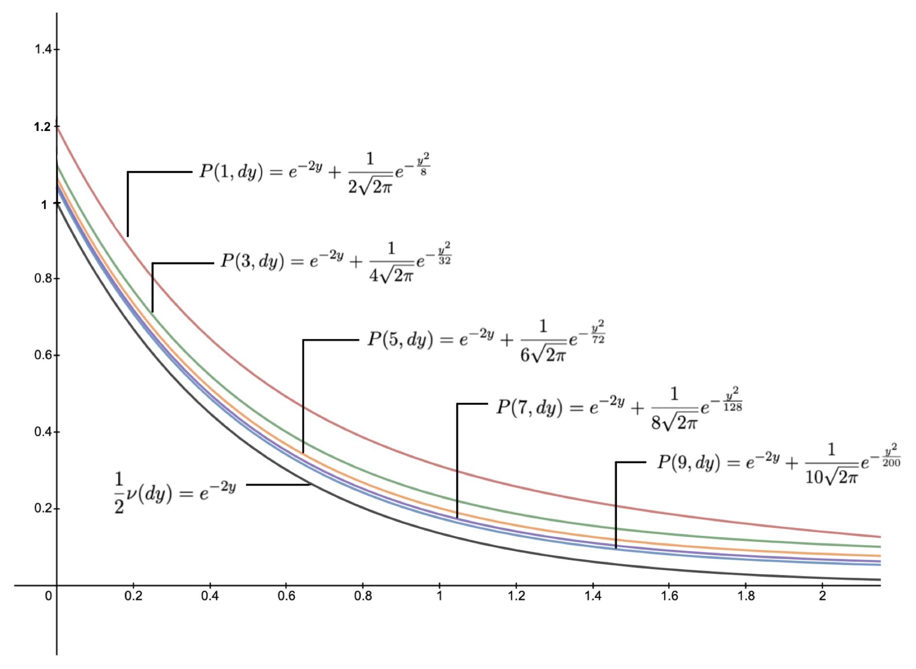
Figure 2: The example satisfying the minorization condition.

The uniform minorization condition implies that there exists a common overlap of size $\epsilon$ between all of the transition probabilities. This allows us to formulate a coupling construction of two different copies $\{X_{n}\}$ and $\{X^{\prime}_{n}\}$ of a Markov chain, as follows. Assume for now that $n_{0}=1$. First, choose $X_{0}\sim\mu_{0}(\cdot)$ and $X_{0}^{\prime}\sim\pi(\cdot)$ independently. Then, inductively for $n=0,1,2,\ldots$,

1. If $X_{n}=X_{n}^{\prime}$, choose $z\sim P(X_{n},\cdot)$ and let $X^{\prime}_{n+1}=X_{n+1}=z$. The chains have already coupled, and they will remain equal forever.

2. If $X_{n}\not=X_{n}^{\prime}$, flip a coin whose probability of Heads is $\epsilon$. If it shows Heads, choose $z\sim\nu(\cdot)$ and let $X^{\prime}_{n+{1}}=X_{n+{1}}=z$. Otherwise, update $X_{n+{1}}$ and $X^{\prime}_{n+1}$ independently with probabilities given by

$${\rm Prob}(X_{n+1}\in A)=\frac{P(X_{n},A)-\epsilon\nu(A)}{1-\epsilon},\quad{\rm Prob}(X^{\prime}_{n+1}\in A)=\frac{P(X^{\prime}_{n},A)-\epsilon\nu(A)}{1-\epsilon}\,.$$

(The minorization condition guarantees that these “residual” probabilities are non-negative, and hence are probability measures since their total mass equals ${P(X_{n},\mathcal{X})-\epsilon\nu(\mathcal{X})\over 1-\epsilon}={1-\epsilon\over 1-\epsilon}=1$.) This construction ensures that overall, ${\rm Prob}(X_{n+1}\in A|X_{n}=x)=P(x,A)$ and ${\rm Prob}(X^{\prime}_{n+1}\in A|X^{\prime}_{n}=x)=P(x,A)$ for any $x\in\mathcal{X}$: indeed, if the two chains are unequal at time $n$, then

$$\begin{split}&{\rm Prob}(X_{n+1}\in A\ |\ X_{n}=x)\\ &={\rm Prob}(X_{n+1}\in A,\,{\rm Heads}\ |\ X_{n}=x)+{\rm Prob}(X_{n+1}\in A,\,{\rm Tails}\ |\ X_{n}=x)\\ &={\rm Prob}({\rm Heads})\ {\rm Prob}(X_{n+1}\in A\ |\ X_{n}=x,\ {\rm Heads})\\ &\qquad\qquad\qquad+{\rm Prob}({\rm Tails})\ {\rm Prob}(X_{n+1}\in A\ |\ X_{n}=x,\ {\rm Tails})\\ &=\epsilon\,\nu(A)+(1-\epsilon)\,\frac{P(x,A)-\epsilon\,\nu(A)}{1-\epsilon}\ =\ P(x,A)\,.\end{split}$$

If $n_{0}>1$, then we can use the above construction for the times $n=0,n_{0},2n_{0},\ldots$, with $n+1$ replaced by $n+n_{0}$, and with $P(\cdot,\cdot)$ replaced by $P^{n_{0}}(\cdot,\cdot)$. Then, if desired, we can later “fill in” the intermediate states $X_{n}$ for $jn_{0}<n<(j+1)n_{0}$, from their appropriate conditional distributions given the already-constructed values of $X_{jn_{0}}$ and $X_{(j+1)n_{0}}$.

Now, since $X^{\prime}_{0}\sim\pi(\cdot)$, and $\pi$ is a stationary distribution, therefore $X^{\prime}_{n}\sim\pi(\cdot)$ for all $n$. And, every $n_{0}$ steps, the two chains probability at least $\epsilon$ of coupling (i.e., of the coin showing Heads). So, ${\rm Prob}(X_{n}\not=X_{n}^{\prime})\leq(1-\epsilon)^{\lfloor n/n_{0}\rfloor}$, where $\lfloor\cdot\rfloor$ means floor. The coupling equality then implies:

Theorem 1.

If $\{X_{n}\}$ is a Markov chain on $\mathcal{X}$, whose transition probabilities satisfy a uniform minorization condition for some $\epsilon>0$, then for any positive integer $n$, and any $x\in\mathcal{X}$,

$$\left\lVert\mathcal{L}(X_{n})-\pi(\cdot)\right\rVert_{TV}\ \leq\ (1-\epsilon)^{\lfloor n/n_{0}\rfloor}.$$

For the above Markov chain (1), we showed a uniform minorization condition with $n_{0}=1$ and $\epsilon=1/2$. So, Theorem 1 immediately implies that $\left\lVert\mathcal{L}(X_{n})-\pi(\cdot)\right\rVert_{TV}\leq(1-\epsilon)^{\lfloor n/n_{0}\rfloor}=(1-(1/2))^{n}=2^{-n}$, which is $<0.01$ if $n\geq 6$, i.e. this chain converges within 6 steps.

If $\mathcal{X}$ is finite, and for some $n_{0}\in{\mathbb{N}}$ there is at least one state $j\in\mathcal{X}$ such that the $j^{\rm th}$ column of $P^{n_{0}}$ is all positive, i.e. $(P^{n_{0}})_{ij}>0$ for all $i\in\mathcal{X}$. Then we can set $\epsilon=\sum_{j\in\mathcal{X}}\min_{i\in\mathcal{X}}(P^{n_{0}})_{ij}>0$, and $\nu(j)=\epsilon^{-1}\,\min_{i\in\mathcal{X}}(P^{n_{0}})_{ij}$, so that $(P^{n_{0}})_{ij}\geq\epsilon\,\nu(j)$ for all $i,j\in\mathcal{X}$, i.e. an $n_{0}$-step uniform minorization condition is satisfied with that value of $\epsilon$.

4.1 Application to Bunny Example

The bunny example does not satisfy a one-step minorization condition, since every column of $P$ has some zeroes, so we instead consider its two-step transition probabilities, $P^{2}$:

In this two-step transition matrix, the fifth column only contains positive values, since no matter where the bunny starts, there will always be at least a $\frac{9}{80}$ chance that it will jump to the center bush ($G5$) in two steps. Thus, we can satisfy a two-step minorization condition by taking

$$\epsilon=\sum_{j\in\mathcal{X}}\min_{i\in\mathcal{X}}(P^{2})_{ij}=0+\dots+0+\frac{9}{80}+0+\dots+0\\ =\frac{9}{80}$$

and $\nu(j)=\epsilon^{-1}\,\min_{i\in\mathcal{X}}(P^{n_{0}})_{ij}$ as above. Then, we can apply Theorem 1, with $n_{0}=2$ and $\epsilon=9/80$, to conclude that

$$\left\lVert\mathcal{L}(X_{n})-\pi(\cdot)\right\rVert_{TV}\ \leq\ \Big{(}1-\frac{9}{80}\Big{)}^{\lfloor n/2\rfloor}=\ \Big{(}\frac{71}{80}\Big{)}^{\lfloor n/2\rfloor}$$

For example, if we want the distribution of the bunny’s location to be within 0.01 of the stationary distribution $\pi$, this is achieved within $n=78$ steps. This bound is not nearly as tight as our previous result $n=6$, but it is uniform over all states (not just $G5$), plus it was derived using a much more general method (without the need to compute eigenvalues and eigenvectors). Of course, such bounds might be more difficult to obtain on larger, more complicated examples.

4.2 Pseudo-Minorization Conditions

The coupling construction used to prove Theorem 1 was a pairwise construction, i.e. it only considered two chain locations $x$ and $y$ at a time. If we replace the distribution $\nu(\cdot)$ with $\nu_{xy}(\cdot)$, allowing it to depend on $x$ and $y$, then $C$ is called a pseudo-small set, and Theorem 1 continues to hold [4]. It then follows that on a finite state space, if we instead choose

$$\epsilon\ =\ \min_{i,j\in\mathcal{X}}\sum_{z\in\mathcal{X}}\min\{(P^{n_{0}})_{iz},(P^{n_{0}})_{jz}\}>0;\quad\nu_{ij}(z)=\frac{\min\{(P^{n_{0}})_{iz},(P^{n_{0}})_{jz}\}}{\sum\limits_{w\in\mathcal{X}}\min\{(P^{n_{0}})_{iw},(P^{n_{0}})_{jw}\}}\,,$$

then the chain will satisfy an $n_{0}$-step pseudo-minorization condition, i.e. for all $i,j,z\in\mathcal{X}$, $(P^{n_{0}})_{iz}\geq\epsilon\,\nu_{ij}(z)$ and $(P^{n_{0}})_{jz}\geq\epsilon\,\nu_{ij}(z)$. Hence, exactly as above, we will again have $\left\lVert\mathcal{L}(X_{n})-\pi(\cdot)\right\rVert_{TV}\,\leq\,(1-\epsilon)^{\lfloor n/n_{0}\rfloor}$.

We now apply this pseudo-minorization idea to the bunny example, with $n_{0}=2$. Examining the matrix $P^{2}$ above, we see that the minimum values of $\sum_{z\in\mathcal{X}}\min\{(P^{2})_{iz},(P^{2})_{jz}\}$ occur at $(i,j)=(3,7)$ or $(1,9)$, corresponding to opposite corners of the $3\times 3$ grid (which makes sense since opposite corners will have the least amount of transitional overlap). We then calculate the minorization constant

$$\epsilon\ =\ \sum_{z\in\mathcal{X}}\min\{(P^{2})_{3z},(P^{2})_{7z}\}\ =\ \frac{1}{12}+0+0+0+\frac{1}{6}+0+0+0+\frac{1}{12}\ =\ \frac{1}{3}\,.$$

Therefore, $\left\lVert\mathcal{L}(X_{n})-\pi(\cdot)\right\rVert_{TV}\,\leq\,(1-\epsilon)^{\lfloor n/2\rfloor}\,=\,(\frac{2}{3})^{\lfloor n/2\rfloor}$. For instance, this bound is $<0.01$ if $n=24$, i.e. if the bunny jumps 24 times. This is a significant improvement over the previous minorization result of $n=78$, though it is still not as tight as the specific eigenvalue bound of $n=6$.

5 Continuous State Space: Point Process MCMC

The above analysis was primarily focused on finite state spaces, such as the bunny example. We now extend to continuous examples on subsets of ${\mathbb{R}}^{d}$.

To be specific, consider a point process consisting of three particles each randomly located within the closed rectangle $[0,1]^{2}\subset\mathbb{R}^{2}$, with positions denoted by $x=(x_{i})_{i=1,2,3}=(x_{i1},x_{i2})_{i=1,2,3}$, so the state space $\mathcal{X}=[0,1]^{6}$. Suppose these particles are distributed according to a probability distribution with unnormalized density (meaning that the actual density is a constant multiple of so it integrates to 1) given by

$$\pi(x)\ :=\ \pi(x_{1},x_{2},x_{3})\ =\ \exp\Big{[}-C\sum_{i=1}^{3}||x_{i}||-D\sum_{i<j}||x_{i}-x_{j}||^{-1}\Big{]}\,,$$

where $C$ and $D$ are fixed positive constants, and $||\cdot||$ is the usual Euclidean ($L^{2}$) norm on $\mathbb{R}^{2}$. In this density, the first sum pushes the particles towards the origin, and the second sum pushes them away from each other.

We now create a Markov chain which has $\pi$ as its stationary distribution. To do this, we use a version of the Metropolis Algorithm [3]. Each step of the Markov chain proceeds as follows. Given $X_{n}=x$, we first “propose” to move the particles from their current configuration $x$ to some other configuration $y$, chosen from the uniform (i.e., Lebesgue) measure on $\mathcal{X}$. Then, with probability $\min[1,\,{\pi(y)\over\pi(x)}]$, we “accept” this proposal and move to the new configuration by setting $X_{n+1}=y$. Otherwise, we “reject” this proposal and leave the configuration unchanged by setting $X_{n+1}=x$.

This Metropolis Algorithm is a well-known procedure which can easily be shown [3, 1] to create a Markov chain which has $\pi$ as its stationary distribution. It is the most common type of Markov chain Monte Carlo (MCMC) algorithm. Such algorithms are a very popular and general method of generating samples from complicated probability distributions, by running the corresponding Markov chain for many iterations. They are used very frequently in a wide variety of fields, ranging from Bayesian statistics to financial modeling to medical research to machine learning and more. For further background, see e.g. [1] and the many references therein.

However, to get reliable samples, it is important to know how many iterations are required to approximately converge to $\pi$, i.e. to establish quantitative convergence bounds. The above Markov chain has an uncountably infinite state space $\mathcal{X}$, so the eigenvalue analysis of Section 3 is not easily available (though there have been some efforts to use spectral analysis on general state spaces, see e.g. [2] and other papers). On the other hand, the uniform minorization condition of Section 4 can still be applied. Indeed, in the web appendix [10], we prove:

Lemma 1.

The Markov chain constructed above satisfies a uniform minorization condition with $n_{0}=1$ and $\epsilon=(0.48)\,e^{-C(4.25)-D(9.88)}$.

For example, if $C=D=1/10$, then we may take $\epsilon=0.117$. It then follows from Theorem 1 that we have the convergence bound

$$\left\lVert\mathcal{L}(X_{n})-\pi(\cdot)\right\rVert_{TV}\ \leq\ (1-\epsilon)^{n}\ =\ (1-0.117)^{n}\ =\ (0.883)^{n}\,.$$

This shows that after $n=38$ steps, the total variation distance between our Markov chain and the stationary distribution will be less than 0.01.

6 Unbounded State Space: Drift Conditions

In the previous section, the uniform minorization condition give us a good quantitative convergence bound. However, in many cases, especially on unbounded state spaces, the minorization condition cannot be satisfied uniformly, only on some subset $C\subseteq\mathcal{X}$. In such cases, we have to adjust our previous $n_{0}=1$ coupling construction, as follows. We first choose $X_{0}\sim\mu(\cdot)$ and $X_{0}^{\prime}\sim\pi(\cdot)$ independently, and then inductively for $n=0,1,2,\ldots$,

1. If $X_{n}=X^{\prime}_{n}$, we choose $X_{n+1}=X^{\prime}_{n+1}\sim P(X_{n},\cdot)$.

2. Else, if $(X_{n},X^{\prime}_{n})\in C\times C$, we flip a coin whose probability of Heads is $\epsilon$, and then update $X_{n+1}$ and $X^{\prime}_{n+1}$ in the same way as in step 2 of our previous (uniform minorization) construction above.

3. Else, if $(X_{n},X^{\prime}_{n})\not\in C\times C$, then we just conditionally independently choose $X_{n+1}\sim P(X_{n},\cdot)$ and $X_{n+1}^{\prime}\sim P(X_{n}^{\prime},\cdot)$, i.e. the two chains are simply updated independently.

The above construction provides good coupling bounds provided that the two chains return to $C\times C$ often enough, but this last property is difficult to guarantee. Thus, to obtain convergence bounds, we also require a drift condition. Basically, the drift condition guarantees that the chains will return to $C\times C$ quickly enough that we can still achieve a coupling.

Definition. A Markov chain with a small set $C\subseteq\mathcal{X}$ satisfies a bivariate drift condition if there exists a function $h:\mathcal{X}\times\mathcal{X}\rightarrow[1,\infty)$ and some $\alpha>1$, such that

$$\bar{P}h(x,y)\leq h(x,y)/\alpha,\quad(x,y)\notin C\times C\,,$$

where

$$\bar{P}h(x,y)\ :=\ {\bf E}[h(X_{n+1},Y_{n+1})\ |\ X_{n}=x,Y_{n}=y]$$

is the expected (average) value of $h(X_{n+1},Y_{n+1})$ on the next iteration, when the chains start from $x$ and $y$ respectively (and proceed independently).

Such bivariate drift conditions can be combined with non-uniform minorization conditions to produce quantitative convergence bounds. To state them, we use the quantity $B_{n_{0}}=\max\{1,\alpha^{n_{0}}(1-\epsilon)\sup_{C\times C}\bar{R}h\}$, where

$$\bar{R}h(x,y)\ =\ \int_{\mathcal{X}}\int_{\mathcal{X}}(1-\epsilon)^{-2}\,h(z,w)\,[P^{n_{0}}(x,dz)-\epsilon\nu(dz)]\,[P^{n_{0}}(y,dw)-\epsilon\nu(dw)]\,.$$

This daunting expression represents the expected value of $h(X_{n+n_{0}},X^{\prime}_{n+n_{0}})$ given that $X_{n}=x$, that $X^{\prime}_{n}=y$, and that the two chains fail to couple at time $n$ (i.e. the corresponding coin shows Tails). We can simplify $\bar{R}h$ in certain situations. For example, if $D$ is a set such that $P^{n_{0}}(x,D)=1$ for all $x\in C$, then since the expected value of a random variable is always less than the maximal value it could take, we have

$$\sup_{(x,y)\in C\times C}\bar{R}h\ \leq\ \sup_{(x,y)\in D\times D}h(x,y)\,.$$

With all that in mind, we have the following result:

Theorem 2.

Consider a Markov Chain on $\mathcal{X}$, with $X_{0}=x$, and transition probabilities $P$. Suppose the above minorization and bivariate drift conditions hold, for some $C\subseteq\mathcal{X}$, $h:\mathcal{X}\times\mathcal{X}\rightarrow[1,\infty)$, probability distribution $\nu(\cdot)$, $\alpha>1$, and $\epsilon>0$. Then for any integers $1\leq j\leq n$, with $B_{n_{0}}$ as above,

$$\left\lVert\mathcal{L}(X_{n})-\pi\right\rVert_{TV}\ \leq\ (1-\epsilon)^{j}+\alpha^{-n}B_{n_{0}}^{j-1}{\bf E}_{Z\sim\pi}[h(x,Z)]\,.$$

Here we give a basic idea of the proof; for more details, see [7, 5]. We create a second copy of the Markov chain with $X^{\prime}_{0}\sim\pi$, and use the above coupling construction. Let $N_{n}$ be the number of times the chain $(X_{n},X_{n}^{\prime})$ is in $C\times C$ by the $n^{\rm th}$ step. Then by the coupling inequality,

$$\left\lVert\mathcal{L}(X_{n})-\pi\right\rVert_{TV}\ \leq\ P[X_{n}\neq X^{\prime}_{n}]\ \leq\ P[X_{n}\neq X_{n}^{\prime},N_{n-1}\geq j]+P[X_{n}\neq X_{n}^{\prime},N_{n-1}<j]\,.$$

The first term suggests that the chains have not coupled by time $n$ despite visiting $C\times C$ at least $j$ times. Since each such time gives them a chance of $\epsilon$ to couple, the first term is $\leq(1-\epsilon)^{j}$. The second term is more complicated, but from the bivariate drift condition together with a martingale argument, it can be shown to be no greater than $\alpha^{-n}B_{n_{0}}^{j-1}{\bf E}_{Z\sim\pi}[h(x,Z)]$.

Sometimes it could be hard to directly check the bivariate drift condition. We now introduce the more easily-verified univariate drift condition, and give a way to derive the bivariate condition from the univariate one.

Definition.

A Markov chain with a small set $C$ satisfies a univariate drift condition if there are constants $0<\lambda<1$ and $b<\infty$, and a function $V:\ \mathcal{X}\rightarrow[1,\infty]$, such that:

$$PV(x)\ \leq\ \lambda V(x)+b\mathbf{1}_{C}(x),\quad x\in\mathcal{X}\,,$$

where $PV(x):={\bf E}[V(X_{n+1})\ |\ X_{n}=x]$.

This univariate drift condition can be used to bound ${\bf E}_{\pi}(V)$. Indeed, assuming ${\bf E}_{\pi}(V)<\infty$, stationarity then implies that ${\bf E}_{\pi}(V)\leq{\bf E}_{\pi}(V)+b$, whence ${\bf E}_{\pi}(V)\leq b/(1-\lambda)$. But also, univariate drift condition can imply bivariate drift conditions, as follows.

Proposition.

Suppose the univariate drift condition is satisfied for some $V:\ \mathcal{X}\rightarrow[1,\infty]$, $C\in\mathcal{X}$, $0<\lambda<1$ and $b<\infty$. Let $d=\inf_{x\in C^{c}}V(x)$. If $d>[b/(1-\lambda)]-1$, then the bivariate drift condition is satisfied for the same C, with $h(x,y)=\frac{1}{2}[V(x)+V(y)]$ and $\alpha^{-1}=\lambda+b/(d+1)<1$.

Proof.

Assume $(x,y)\notin C\times C$. Then either $x\notin C$ or $y\notin C$, so $h(x,y)\geq(1+d)/2$. Then, our univariate drift condition applied separately to $x$ and to $y$ implies that $PV(x)+PV(y)\leq\lambda V(x)+\lambda V(y)+b$. Therefore

$$\bar{P}h(x,y) =\frac{1}{2}[PV(x)+PV(y)]\leq\frac{1}{2}[\lambda V(x)+\lambda V(y)+b]=\lambda h(x,y)+b/2$$

$$\leq\lambda h(x,y)+(b/2)[h(x,y)/((1+d)/2)]=[\lambda+b/(1+d)]h(x,y)\,,$$

which gives the result. ∎

We now apply these non-uniform quantitative convergence bounds to a Markov chain on an unbounded state space. Let the state space be $\mathcal{X}=\mathbb{R}$, the entire real line, with unnormalized target density $\pi(x)=e^{-|x|}$.

To create a Markov chain which has $\pi$ as its stationary distribution, we use another version of the Metropolis Algorithm [3, 1]. Each step of the Markov chain proceeds as follows. First, we propose to move from the state $x$ to some other state $y$, chosen from the uniform (i.e., Lebesgue) measure on the interval $[x-2,x+2]$. Then, with probability $\min[1,\ {\pi(y)\over\pi(x)}]$, we accept this proposal and move to the new state $y$, otherwise we reject it and remain at $x$. Once again, this procedure creates a Markov chain which has $\pi$ as its stationary distribution.

To apply Theorem 2, we need to establish minorization and drift conditions. In the web appendix [10], we prove:

Lemma 2.

The above Markov chain satisfies a minorization condition with $C=[-2,2]$, $n_{0}=2$, $\epsilon={1\over 8e^{2}}$, and $\nu(A)={1\over 2}\,{\rm Leb}(A\cap[-1,1])$, where ${\rm Leb}$ is Lebesgue measure on ${\mathbb{R}}$.

Lemma 3.

The above Markov chain satisfies a univariate drift condition with $V(x)=e^{-|x|/2}$, $C=[-2,2]$, $\lambda=0.916$, and $b=0.285$.

We can then apply the above Proposition to derive a bivariate drift condition. Note that here $d=\inf_{x\in C^{c}}V(x)=e$, and $[b/(1-\lambda)]-1=2.39<e$. So, $h(x,y):=\frac{1}{2}(V(x)+V(y))$ satisfies a bivariate drift condition with $\alpha^{-1}=\lambda+b/(d+1)=0.916+0.285/(e+1)\doteq 0.993$.

We also need to bound the above quantity $B_{n_{0}}=B_{2}$. Let $D=[-6,6]$. Then clearly $P^{2}(x,D)=1$ for any $x\in C$. Thus

$$\sup_{(x,y)\in C\times C}\bar{R}h(x,y)\ \leq\ \sup_{(x,y)\in D\times D}h(x,y)\ =\ \sup_{x\in D}V(x)\ =\ e^{3}\ <\ 20.1\,.$$

So $B_{2}\equiv\max[1,\alpha^{2}(1-\epsilon)\sup\bar{R}h]<(0.993)^{-2}(1-{1\over 8e^{2}})(20.1)\doteq 20.04$.

Let $X_{0}=0$. Then

$${\bf E}_{Z\sim\pi}[h(0,Z)]\ =\ {\bf E}_{Z\sim\pi}[\frac{1}{2}(V(0)+V(Z))]\ =\ \frac{1}{2}+{1\over 2}{\bf E}_{\pi}(V)\\ \ =\ \frac{1}{2}+{1\over 2}\frac{\int_{y\in\mathcal{X}}e^{\frac{1}{2}|y|}e^{-|y|}dy}{\int_{y\in\mathcal{X}}e^{-|y|}dy}\ =\ {1\over 2}+{1\over 2}\times\frac{2}{1}\ =\ 2\,.$$

(If this specific calculation were not available, then we could instead use the bound ${\bf E}_{\pi}(V)\leq b/(1-\lambda)=0.285/(1-0.916)=3.393$ as discussed above.) Therefore, by Theorem 2, with $X_{0}=0$, we have

$$\left\lVert\mathcal{L}(X_{n})-\pi\right\rVert_{TV}\ \leq\ (1-\epsilon)^{j}+\alpha^{-n}B_{2}^{j-1}{\bf E}_{Z\sim\pi}[h(0,Z)]\\ \ \leq\ (0.983)^{j}+(0.993)^{n}(20.04)^{j-1}[2]\,.$$

For example, setting $n=120,000$ and $j=274=1+n/439.56$, this becomes $\left\lVert\mathcal{L}(X_{n})-\pi(\cdot))\right\rVert_{TV}\ \leq\ (0.983)^{274}+[(0.993)(20.04)^{1/439.56}]^{120000}[2]\,<\,0.01\,,$ i.e. the Markov chain is within 0.01 of stationarity after 120,000 iterations. This is quite a conservative upper bound. Nevertheless, we have obtained a concrete quantitative convergence bound, for an unbounded Markov chain.

7 Conclusion

This paper has discussed Markov chains and their convergence rates, and why they are important for MCMC algorithms. We introduced the eigenvalue method, the coupling method, and minorization and drift conditions, and applied them to examples on state spaces ranging from finite to compact to unbounded. For the bunny example, we showed several possible methods of obtaining convergence bounds. Indeed, bounding a Markov chain’s convergence rate is not an one-time, definitive process; for various Markov chains, it is possible to strengthen the bound through careful and creative new constructions. The bounds presented in this paper all have their imperfections, and will certainly not give tight or realistic bounds for all examples. There is plenty of room for new and tighter and more flexible bounds, which can help us to understand Markov chains better, and also run MCMC algorithms more confidently and reliably.

Acknowledgements. We thank the editor and reviewers for very helpful comments on the first version of this manuscript.

References

- [1] Brooks, S., Gelman, A., Jones, G., and Meng, X.-L., eds. (2011), Handbook of Markov chain Monte Carlo. Chapman & Hall, New York.
- [2] C.J. Geyer (1992), Practical Markov chain Monte Carlo. Statistical Science 7, 473–483.
- [3] Metropolis, N., Rosenbluth, A.W., Rosenbluth, M.N., Teller, A.H., and Teller, E. (1953). Equation of state calculations by fast computing machines. The Journal of Chemical Physics 21(6), 1087–1092.
- [4] Roberts, G.O. and Rosenthal, J.S. (2001), Small and Pseudo-Small Sets for Markov Chains. Stochastic Models 17, 121–145.
- [5] Roberts, G.O. and Rosenthal, J. S. (2004). General State Space Markov Chains and MCMC Algorithms. Probability Surveys 1, 20–71.
- [6] Rosenthal, J.S. (1995). Convergence Rates for Markov Chains. SIAM Review 37(3), 387–405.
- [7] Rosenthal, J.S. (2002). Quantitative Convergence Rates of Markov Chains: A Simple Account. Electronic Communications in Probability 7, 123–128.
- [8] Rosenthal, J.S. (2019). A First Look at Stochastic Processes. World Scientific Publishing Company, Singapore.
- [9] Thorisson, H. (2000). Coupling, Stationarity, and Regeneration. Springer, New York.
- [10] Web Appendix for this paper. Available at: www.probability.ca/NoticesApp