DiverseNet: When One Right Answer is not Enough^†

Abstract

Many structured prediction tasks in machine vision have a collection of acceptable answers, instead of one definitive ground truth answer. Segmentation of images, for example, is subject to human labeling bias. Similarly, there are multiple possible pixel values that could plausibly complete occluded image regions. State-of-the art supervised learning methods are typically optimized to make a single test-time prediction for each query, failing to find other modes in the output space. Existing methods that allow for sampling often sacrifice speed or accuracy.

We introduce a simple method for training a neural network, which enables diverse structured predictions to be made for each test-time query. For a single input, we learn to predict a range of possible answers. We compare favorably to methods that seek diversity through an ensemble of networks. Such stochastic multiple choice learning faces mode collapse, where one or more ensemble members fail to receive any training signal. Our best performing solution can be deployed for various tasks, and just involves small modifications to the existing single-mode architecture, loss function, and training regime. We demonstrate that our method results in quantitative improvements across three challenging tasks: $2$D image completion, $3$D volume estimation, and flow prediction.

1 Introduction

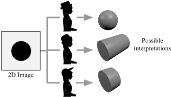
Computer vision systems are typically trained to make a single output prediction from a given input. However, in many cases, there is more than one correct answer. Consider the case of $3$D projection in Figure 1. We wish to infer what $3$D shape projected to form a given $2$D silhouette. The training data suggests that there should be more than one answer: some users identify the circle as being produced by a sphere, while others hypothesized different sized cylinders, viewed head-on. We assert that each of these interpretations is correct, and, depending on the application scenario, different outputs may be required. However, a typical neural network predictor might make a single prediction which averages together the modes present (Figure 1(b), top).

(a) Many prediction tasks have ambiguous interpretations. For example, giving a 2D rendering to a human, there are different possible 3D interpretations.

(b) Standard CNNs trained under multi-modal labels tend to blur together or ignore the distinct modes. We introduce a modification to standard neural networks that gives the user a control parameter $\mathbf{c}$. Different values of $\mathbf{c}$ produce diverse structured outputs for the same input.

Figure 1: Our easy modification enhances typical loss functions, producing networks that predict multiple good answers, not just one best-majority-fit output. Access to “minority” outputs is especially useful in applications dealing with ambiguous completions or human preferences.

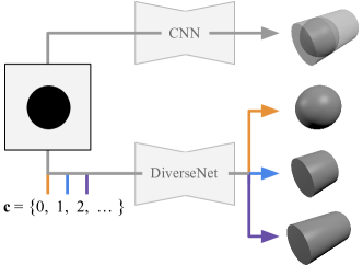
While many machine learning systems are able to produce samples at test time (e.g. [9, 17, 34]), we propose a method which explicitly exploits diversity in training labels to learn how to make a range of possible structured predictions at test time. Our system is an add-on modification of the loss function and training schedule that is compatible with any supervised learning network architecture. Our contributions allow for a network to take as input a test image $\mathbf{x}$ and a control parameter $\mathbf{c}$. Where training time diversity exists, our loss encourages the network to find the different modes in the label space. At test time, providing the same $\mathbf{x}$ with different values of $\mathbf{c}$ produces different predictions (Figure 1(b)). Our method can be applied to any supervised learning architecture and loss.

Our method is also applicable in cases where there is one definitive ground truth answer. For example, a grayscale image has a single ground truth colorization; however, for most applications a user may be satisfied with a range of plausible suggestions [26, 27]. Our method can predict diverse solutions even where only one label exists for each training item.

Our main contribution is an architecture-modification and loss which prevent mode-dropping. Mode-dropping is a phenomenon recently observed in GAN training [37], where regions of output space are not reached by predictions from a model. We observe this effect in [23]; during training, their method can result in some members of the ensemble failing to receive any training signal. This occurs when other ensemble members are much closer to the mean of the output space. At test time, those ensemble members fail to make a meaningful prediction. Our method avoids this problem.

2 Related work

There is a large body of work that examines the cases where labels for data are diverse, noisy or wrong [19, 30, 35]. Most of these, however, assume that the labels are a noisy approximation of one true label, while we assume they are all correct. Methods which make diverse predictions can be roughly categorized as: (a) those which allow for sampling of solutions; (b) ensembles of models, each of which can give a different prediction, and (c) systems which find diverse predictions through test-time optimization.

Sampling methods

Where parameters are learned as parametric distributions, samples can be drawn; for example, consider the stochastic binary distribution in the case of Boltzmann Machines [1]. Restricted Boltzmann Machines [12], Deep Boltzmann Machines [34] and Deep Belief Networks (DBNs) [13] are all generative methods that learn probabilistic distributions over interactions between observed and hidden variables. Such probabilistic networks allow samples to be drawn from the network at test time using MCMC methods such as Gibbs Sampling. This has been used, for example, to sample 2D and 3D shape completions [8, 43]. Unfortunately, these sampling processes are often time consuming resulting in models that are difficult to train (as the models scale) and expensive to sample.

Removing the stochastic nature of the units, the supervised learning scheme for DBNs leads to autoencoders [14] that are easier to train but the directed model no longer maintains distributions and therefore cannot be sampled from. Variational autoencoders (VAEs) [17] use a variational approximation to estimate (Gaussian) distributions over a low dimensional latent space as a layer in the predictive network. These distributions capture uncertainty in the latent space and can, therefore, be sampled at test time. However, the smooth local structure of the latent space makes it unlikely to capture different modes; instead the variational approximation is targeted towards complexity control on the dimensionality of the latent space.

Generative adversarial networks (GANs) have an optimization scheme which enables novel data to be sampled  [10], possibly conditioned on an input sample [29]. Unsupervised control can be enabled with an extra input, which is encouraged to correlate with the generated image [6]. This method is restricted to use with GANs, while our method can be added to any supervised loss. Like [6], though, we find the relationship between the controlling input and modes in the output space automatically, and we control the output space via an additional input ($\mathbf{c}$).

Figure 2: A toy example showing our update formulation as applied to image segmentation. Here, the image $\mathbf{x}$ has four $\mathbf{y}$ labels associated with it. (1) Forward pass On the forward pass, the same $\mathbf{x}$ is provided to the network $N$ times, each time with a different value for $\mathbf{c}$. Each of the outputs produced is different due to the different values of $\mathbf{c}$. (2) Backward pass We associate each ground truth label $\mathbf{y}\in\mathcal{Y}$ with its best matching network output. This matching is indicated by the solid arrows. Losses are then backpropagated only for these values of $\mathbf{c}$. The paths along which gradient flows are shown by dashed arrows. (3) Next epoch When the same $\mathbf{x}$ and $\mathbf{c}$ values are passed to the network on the next epoch, each prediction is now a little more like the ground truth image it was matched with.

Ensembles

Ensembles of neural networks have been found to outperform networks in isolation [20]. Typically, each network is trained on all the training data, allowing randomness in initialization and augmentation to lead each network to a distinct local minimum. Bagging, where each classifier is trained on a random subset of the training data, can be used to increase the variance of prediction from multiple weak classifiers [5]. Alternatively, Liu and Yao [24] explicitly encourage diversity in the ensemble by the addition of a variance term to the loss function that forces solutions apart from each other, and similarly Dey et al. [7] train a sequence of predictors explicitly to give diverse predictions. As far as Dropout [38] can be considered to approximate an ensemble [3], then its application at test time [9] can be considered as drawing samples from a large ensemble.

Lee et al. [22, 23] introduce a loss which encourages ensemble diversity. They backpropogate the loss for each training example only through the ensemble member that achieves the best loss on the forward pass. Each network, over time, becomes an “expert” in a different field. Their loss, which is based on [11], is related to ours. We differ in three ways. First, they train an ensemble (or quasi-ensemble, ‘treenet’) of networks, while we make multiple predictions from a single network, significantly reducing the number of parameters. Second, their loss does not directly take advantage of training time diversity, while ours handles cases both where we do and do not have multiple labels for each training item. Third, as introduced in Section 1, our approach prevents mode-dropping [37].

Test-time diversity

Some methods explicitly enforce diverse modes at test time. For example, Batra et al. [4] find diverse solutions for a Markov random field with a greedy method which applies a penalty to each new solution if it agrees too much with previously discovered modes. This was subsequently developed to a more general solution [18]. In contrast, ours learns at training time how to make diverse predictions; each prediction is then made with a single network evaluation.

3 Method

Typically, training data for supervised learning consists of a set of pairs $\mathcal{D}=\{(\mathbf{x},\mathbf{y})\}$. Each pair consists of an input $\mathbf{x}$, which in vision tasks is often an image, and the desired output label $\mathbf{y}$; for our structured prediction tasks, $\mathbf{y}$ is multidimensional. Training the parameters of a machine learning system $f$ then involves minimizing a loss $l$ summed over this set of data, i.e.

$$L=\sum_{(\mathbf{x},\mathbf{y})\in\mathcal{D}}l(f(\mathbf{x}),\mathbf{y}).$$ (1)

In our work, we assume that for each $\mathbf{x}$ there is a set of labels. Each training pair $(\mathbf{x},\mathcal{Y})$ now comprises a single $\mathbf{x}$ with a set of target values $\mathcal{Y}=\{\mathbf{y}_{1},\mathbf{y}_{2},\ldots\mathbf{y}_{N}\}$. For example, for image segmentation each image may have had boundaries drawn by multiple human labelers. Note that $N$ can be different for different training pairs. A straightforward modification of (1) to minimize the loss over $\mathcal{Y}$ is

$$L=\sum_{(\mathbf{x},\mathcal{Y})\in\mathcal{D}}\,\,\sum_{\mathbf{y}\in\mathcal{Y}}l(f(\mathbf{x}),\mathbf{y}).$$ (2)

Unfortunately, using (2) explicitly (or averaging the label set, which is often done in practice), results in predictions being made that lie between modes in the label space. This “mode collapse” effect has been observed when training networks on ambiguous tasks like image completion [31].

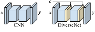
Our model instead accepts as input $\mathbf{x}$ together with a control variable $\mathbf{c}\in\mathcal{C}$. Specifically, $\mathbf{c}$ is fed to the network through concatenation with activations from both dense and convolutional layers, and integer values for $\mathbf{c}$ are first converted to a one-hot representation. At test time, users can create different outputs for the same $\mathbf{x}$ by varying the value of $\mathbf{c}$ (Figure 1(b)).

We assume that, during training, each $\mathbf{y}\in\mathcal{Y}$ is a valid output that we wish our system to be able to reconstruct under at least one value of $\mathbf{c}$. For a single $\mathbf{x},\mathbf{y}$ pair, the value of $\mathbf{c}$ which produces a network output that most closely matches $\mathbf{y}$ is $\operatorname*{arg\,min}_{\mathbf{c}\in\mathcal{C}}\,\,l(f(\mathbf{c},\mathbf{x}),\mathbf{y})$. We want each $\mathbf{y}\in\mathcal{Y}$ to be well reconstructed, so we penalize any $\mathbf{y}$ which is not well reconstructed by $f$. Our loss is therefore

$$L_{\text{div}}=\sum_{(\mathbf{x},\mathcal{Y})\in\mathcal{D}}\,\,\sum_{\mathbf{y}\in\mathcal{Y}}\,\,\min_{\mathbf{c}\in\mathcal{C}}\,\,l(f(\mathbf{c},\mathbf{x}),\mathbf{y}).$$ (3)

We show an illustrative example of an update for a single $(\mathbf{x},\mathcal{Y})$ in Figure 2. On the forward pass through the network, the same $\mathbf{x}$ is passed with different values of $\mathbf{c}$. At this stage in the training, the network produces different results for each value of $\mathbf{c}$. We then associate each possible label, i.e. each $\mathbf{y}\in\mathcal{Y}$ with just one of the network outputs. The losses for these ground truth labels are then backpropagated through the network to the appropriate value of $\mathbf{c}$. After the update, each value of $\mathbf{c}$ is more closely associated with a different mode in the data. This update formulation is a multi-label, single-network extension of [22, 23].

Equation 3 can be implemented easily. For each group of inputs to the network, we compute a matrix measuring the pairwise loss between each network output and each $\mathbf{y}\in\mathcal{Y}$. The min down each column gives the closest matching prediction to each $\mathbf{y}$. The sum over all such min values gives the objective $L_{\text{div}}$.

Preventing mode collapse

We sometimes find that when $|\mathcal{C}|$ is larger than the number of modes naturally present in the data, then one or more values of $\mathbf{c}$ can produce poor solutions. This occurs when, during stochastic training, the modes in the label space are better captured by a subset of $\mathbf{c}$ values, and therefore other values for $\mathbf{c}$ are never encouraged to produce any meaningful result. To remove this undesirable effect, and to help ensure that no predictions are degenerate, we propose an additional term which ensures that the worst performing prediction gets updated, regardless of its proximity to any ground truth label, as

$$L_{\text{catchup}}=\frac{1}{|\mathcal{C}|}\sum_{(\mathbf{x},\mathcal{Y})\in\mathcal{D}}\,\,\max_{\mathbf{c}\in\mathcal{C}}\,\,\min_{\mathbf{y}\in\mathcal{Y}}\,\,l(f(\mathbf{c},\mathbf{x}),\mathbf{y}).$$ (4)

The $\min$ in (4) finds, for each network prediction, the distance to its closest matching ground truth label in $\mathcal{Y}$. The $\max$ then ensures that only the value of $\mathbf{c}$ corresponding to the largest of these losses is updated.

Our final training loss is simply $L=L_{\text{div}}+\beta L_{\text{catchup}}$, where $\beta$ is a parameter which trades off the quality of the best reconstructions ($L_{\text{div}}$) with the worst ($L_{\text{catchup}}$). All the results in this paper are produced with $\beta=1$; we examine the effect of tuning this parameter in Section 4.1.

Learning without training-time diversity

Given only a single label for each training image, i.e. $|\mathcal{Y}|=1$, we can still use our system to make diverse predictions. Our loss function now becomes:

$$L_{\text{div}}=\sum_{(\mathbf{x},\mathbf{y})\in\mathcal{D}}\,\,\min_{\mathbf{c}\in\mathcal{C}}\,\,l(f(\mathbf{c},\mathbf{x}),\mathbf{y}).$$ (5)

This shares similarities with a single-network version of the multiple choice learning loss of [11, 22]. However, our formulation shares parameters across each value of $\mathbf{c}$, resulting in considerably fewer parameters than an ensemble.

Architecture details

We insert categorical $\mathbf{c}$ into the network by converting to one-hot encoding, and concatenating with the activations (Figure 6). We can also use continuous or multi-dimensional values for $\mathbf{c}$. A continuous $\mathbf{c}$ could be useful for example when exploring continuous qualitative artistic options, e.g. using a deep-learned ‘Photoshop’ to complete missing image regions. In these cases it becomes intractable to enumerate all possible values in a single minibatch. Instead, we take a stochastic approximation to (3), and set $\mathcal{C}$ as a set of samples from a user-specified distribution. Our method is applicable to all supervised network architectures, including those with skip connections, dropout, and batch normalization.

Figure 3: Creating MNIST${}_{\text{OCC}}$. Each original MNIST digit (left) is occluded to create an $\mathbf{x}$ image. The $8$ matching digits which most closely match $\mathbf{x}$ form the set $\mathcal{Y}$.

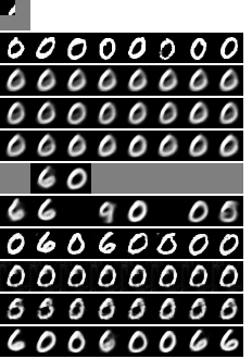
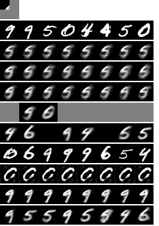
$\mathbf{x}$ (Network input) $\mathcal{Y}$ (Ground truth) (A) $L_{2}$ (B) Dropout (C) Bagged (D) Lee et al. (E) Lee et al. + $\epsilon L_{2}$ (F) GAN sample (G) Cond. GAN (H) VAE Ours

Figure 4: Predictions from the models. For each model, described in Section 4.1, we make $8$ predictions on each image. The ground truth row shows the $\mathcal{Y}$ values in MNIST${}_{\text{OCC}}$, found from the test set using nearest neighbor lookup — the left-most value in $\mathcal{Y}$ is the image from which $\mathbf{x}$ was generated. More results are given in the supplementary material.

4 Experiments

Most networks can be augmented to become a DiverseNet, so we perform experiments across a range of datasets, loss functions, and applications, to demonstrate the generalizability of this approach. We validate that it copes with non-unique labelings and improves diversity against competing diversity-seeking methods. Further, we establish that our models have fewer parameters (almost as few as a native network) and so are easier to train than methods like [23]. Nonetheless, we sacrifice very little accuracy compared to single-best models (Note: like class-imbalance problems, some reduction in raw accuracy is expected).

Evaluating diverse predictions

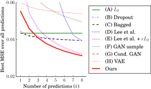
Where only a single ground truth answer exists, the k-best oracle [11, 23] is a suitable scheme for evaluating diverse predictions. For each input, $k$ random predictions are made, and the one which most closely matches the ground truth is chosen. This error is averaged over all test inputs to report the overall error for a particular value of $k$. Sweeping $k$ allows us to plot a graph, where error typically reduces as $k$ is incremented and more predictions are made.

Where there are multiple ground truth answers for each data point, a perfect algorithm would generate each of the ground truth answers. An error is computed for each possible ground truth answer, where again we compare to the closest match among $k$ predictions from the model. The final error is the mean of all these errors.

4.1 Comparing to baselines on MNIST${}_{\text{OCC}}$

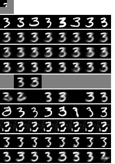
We use the MNIST dataset [21] to demonstrate how our system can be used to find distinct outputs where there is ambiguity at training time. We create a modified occluded version of the dataset, MNIST${}_{\text{OCC}}$, designed for training and evaluating image completion where there are multiple correct answers (Figure 3). Each $\mathbf{x}$ in MNIST${}_{\text{OCC}}$ comprises an original MNIST digit, where all pixels are set to zero except the $14\times 14$ square in the top-left corner of the image. For each $\mathbf{x}$ we must synthesize a diverse set of labels $\mathcal{Y}$. After cropping, we find the $8$ closest matching $\mathbf{x}$ values in the corresponding training set. Their respective associated $\mathbf{y}$ values form the set $\mathcal{Y}$. The aim of this image completion task is to accurately recover $\mathcal{Y}$ given a single $\mathbf{x}$.

For all MNIST${}_{\text{OCC}}$ experiments, unless stated otherwise, we use a simple bottleneck architecture (Figure 6). We train our algorithm with $N=8$ discrete values for $\mathbf{c}$, and for all competing methods we draw $8$ samples. Networks which use $\mathbf{c}$ as input have it concatenated with the activations as a one-hot encoding, as described above. For each baseline, we train with $\mathbf{x}$ against all values of $\mathcal{Y}$. We compare against the following baselines:

Figure 5: Quantitative results on MNIST${}_{\text{OCC}}$. As more predictions are made from the model, the oracle performance of all systems except (A) $L_{2}$ improves.

Figure 6: DiverseNet’s architecture differs from a standard CNN through concatentations of $\mathbf{c}$ with the network activations. $\mathbf{c}$ is typically a one-hot encoding of the integer parameter.

(A) Standard $L_{2}$ loss

A bottleneck architecture, trained with $L_{2}$ reconstruction loss between the input and output.

(B) Test-time Dropout [9, 38]

We train a single network with Dropout applied to the dense layers. At test time, we sample $N$ predictions with different dropout values.

(C) Bagged ensemble

We train an ensemble of $N$ networks, each trained on a random $2/3$ of the training set. At test time, each network gives a single prediction.

(D) Lee et al. ensemble

We form a ‘treenet’ ensemble trained in unison as described in [22] (see Section 2); each ensemble member shares weights in the encoder, but has separate weights in the dense layers and decoder.

(E) Lee et al. ensemble + $\epsilon L_{2}$

We found that several ensemble members in (D) failed to learn, giving null predictions. By adding a small ($10^{-4}$) amount of $L_{2}$ loss we reduced the number of degenerate members and improved their scores.

(F) GAN samples

For this simple baseline we sample $20,000$ images from a GAN [10] trained on MNIST. For each test $\mathbf{x}$, the $k$ samples which most closely match the unmasked corner are taken as the predictions.

(G) Conditional GAN [29]

Here the generator network is trained to produce samples conditioned on $\mathbf{x}$. We use our bottleneck architecture, with a noise vector concatenated on the bottleneck and batch normalization [15] for stability. Different noise samples give each test-time completion.

(H) Variational Autoencoder

Here we make the architectural change of including a Gaussian sampling step in the bottleneck, implemented and trained as [17]. Test-time samples are produced by sampling from the Gaussian.

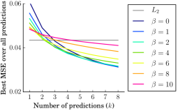
Quantitative results are shown in Figure 5. When making just one or two predictions, our method has a higher MSE than methods trained with an $L_{2}$ loss. However, beyond $3$ predictions, we outperform all competitors. Figure 4 shows qualitative results. The bagged ensemble (C) performs well, as expected, while (D) [22] produces poor results. Qualitative inspection shows that, on this task, some of their ensemble members never produce meaningful results. We see how their method is hurt by dropping modes. Our $L_{\text{catchup}}$ loss helps to prevent this mode dropping. We note that conditional GANs produce highly correlated samples, as observed in [16, 28], since the network learns to ignore the noise input. The sharpness of (F) GAN sample suggests that an adversarial loss could help improve the visual quality of our results.

Continuous values for $\mathbf{c}$

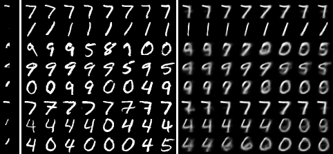
Figure 7 shows image completions from a continuous value of $\mathbf{c}$. Treating $\mathbf{c}$ as a continuous variable has the effect of ordering the completions, and allowing them to be smoothly interpolated. This can, however, lead to implausible completions between modes, e.g. in the final row where the $4$ merges into a $6$.

$\mathbf{x}$                    $\mathcal{Y}$                  $-1\,\,\longleftarrow\,\,\longleftarrow\,\,\mathbf{c}\,\,\longrightarrow\longrightarrow\,\,1$

Figure 7: Image completions using our algorithm with continuous values of $\mathbf{c}$. The first two columns show the input occluded $\mathbf{x}$ values and the ground truth set of $\mathcal{Y}$ values. On the right we show completions on this test image as $\mathbf{c}$ is swept from $-1$ to $1$.

The effect of adjusting $\beta$

All results shown in this paper use $\beta=1$ (Section 3). Figure 8 shows the quantitative effect of adjusting this parameter. As $\beta$ increases, the curves tend toward the $L_{2}$ result; i.e. error is improved for fewer samples, at the expense of reduced diversity. A user of our system may wish to choose $\beta$ to suit the task at hand.

Figure 8: The effect of varying $\beta$ on the MNIST dataset. We include the results for $L_{2}$ (in gray) for comparison with Figure 5. In general, we can see that as $\beta$ increases, the line tends towards the $L_{2}$ result; i.e. error is improved for fewer samples, at the expense of reduced diversity.

Figure 9: Traffic flow dataset. Given an image of road junction (a), and some prior knowledge (e.g. that this image is from a country with left-hand-traffic), one can envisage different patterns of traffic motion that might be expected. For example, (b) shows two-way traffic; (c) shows two-way traffic plus a left filter, etc.

4.2 Predicting traffic flows

Figure 10: Predictions on traffic flow dataset. On the left is the input to our algorithm, a median image from a short traffic camera video. Test cameras are excluded from training. In the center are four flow predictions from our model, made only from the single test-time frame, while the right shows four of the many flow-fields actually observed by this traffic camera. In (a) our system predicts different volumes of traffic flowing in each direction of this two-way road. (b) shows a junction. As well as traffic flowing in each direction, we see traffic leaving (column 3) and joining (column 4) the main road. Here, column 2 predicts no traffic flowing, which is often the case in these short video clips. In (c), we correctly identify the road as a one-way street (cols. 3 and 4) with a separate road crossing the main flow (col. 1).

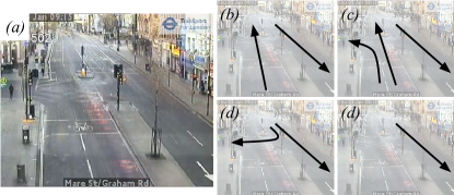
City traffic can exhibit diverse behaviors. In this experiment, we tackle the problem: given a single image of a new road or intersection, can we predict what flow patterns the traffic may exhibit? Consider the image of the traffic intersection in Figure 9. Based on our knowledge, we can predict how traffic might move, were it to be present. There are many correct answers, depending on the phase of the traffic lights, traffic density, and the whims of individual drivers.

$k=$	1	2	3	4
Lee et al.	0.313	0.215	0.172	0.158
$L_{2}$ + test-time Dropout	0.209	0.194	0.187	0.184
Ours	0.203	0.174	0.158	0.146

Table 1: Flow prediction evaluation. Lower numbers are better. Here, we report the best endpoint error over all the predictions made from each model, evaluated against each ground truth flow image. We see that as more predictions are made, all methods improve, while our full method outperforms the baselines.

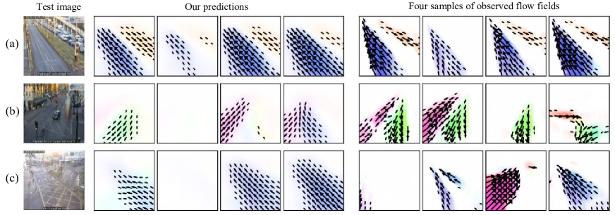
We created a dataset to learn about traffic flows, formed from short ($\scriptstyle\sim$8s) videos taken from a publicly accessible traffic camera network [40]. Each of the 912 traffic cameras in the network continuously films road traffic from a fixed viewpoint, and short clips of traffic are uploaded to their servers every five minutes. We obtained a total of 10,527 distinct videos, around 11.5 videos for each camera location. For each video, we compute the average frame-to-frame optical flow (using [41]) as a single $\mathbf{y}$ pattern. We use a simple bottleneck architecture based on VGG16 [36] — see supplemental materials for details. We divide the camera locations into an 80/20 train/test split. To evaluate, we use the average endpoint error, as advocated by [2]. On this task, we find that each of [23]’s ensemble members produces a meaningful output, so we do not include $\epsilon L_{2}$. We report results compared to [23] and test-time dropout, as those were the best competitors from Section 4.1. Quantitative comparisons are given in Table 1. We outperform the baselines, and representative results are depicted in Figure 10. Note that while infinite combinations of vehicle-motion are possible (within physical limits), our predictions seek to capture the diverse modes, and to associate them with the appearance of regions in a single image. Our diverse predictions capture (a) different directions in the major flow of traffic, (b) different densities of traffic flow, and (c) traffic flow into and from side roads.

4.3 ShapeNet volumes from silhouettes

3D volume prediction from 2D silhouettes has recently become a popular task [42, 33]. However, it is an inherently ambiguous problem, as many different volumes could produce any given silhouette image. This task calls for diverse predictions: we expect that a diverse prediction network will be able to produce several different plausible 3D shape predictions for a given silhouette input.

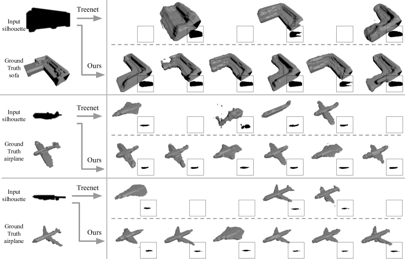
We used a subset of three classes from ShapeNet [44], airplane, car and sofa, and we trained a system to predict the $32^{3}$ voxel grid given a single 2D silhouette rendering as input. Training and testing silhouettes were rendered with a fixed elevation angle ($0^{\circ}$) with azimuth varying in $15^{\circ}$ increments. We trained our model and baselines to produce 6 outputs at test time. Details of architectures are given in the supplemental material. Results are summarized in Table 2 and a few samples illustrated in Figure 11. Our results are typically better, and are achieved with far fewer parameters.

Examining the effect of architecture and loss

We performed an ablation study to discover if the prevention of mode-dropping from our method comes about due to our architecture, or our $L_{catchup}$ loss. We directly compared the ShapeNet results when training with our architecture vs Treenet, and for each architecture we turned $L_{catchup}$ on and off. We also tried pretraining the networks (with the standard loss), to help each ensemble member to produce plausible outputs. We find that, numerically, our proposed method (indicated with $\Rightarrow$) outperforms all other variants.

Measuring plausibility of predictions

In this task, one method of assessing overall plausibility of the predictions is to measure their compatibility with the input silhouettes. The intuition is that good predictions will match with the input silhouette, even if they don’t necessarily match the ground truth. We convert each predicted grid to a mesh [25] and render using the same camera parameters used to create the original silhouette. This is compared to the input silhouette using the IoU, and the average over all of these IoU measures is given in Table 2. The Treenet architecture tends to give a lower re-projection IoU than equivalent predictions from our architecture. This is because of mode dropping; predictions from their network are not always plausible.

Architecture	Params	Test-time		$L_{catchup}$	Pretrain	k=1	k=2	k=3	k=4	k=5	k=6	Reproj	Var
Treenet [23]	66.8M	0.047s				0.296	0.376	0.435	0.482	0.518	0.545	0.313	0.060
				$\bullet$		0.650	0.665	0.676	0.683	0.689	0.694	0.726	0.015
					$\bullet$	0.363	0.454	0.516	0.558	0.586	0.607	0.502	0.059
				$\bullet$	$\bullet$	0.666	0.679	0.688	0.694	0.700	0.704	0.733	0.013
DiverseNet	12.6M	0.053s				0.661	0.680	0.692	0.701	0.708	0.713	0.773	0.014
			$\Rightarrow$	$\bullet$		0.680	0.693	0.702	0.708	0.713	0.716	0.753	0.010
					$\bullet$	0.650	0.669	0.682	0.692	0.698	0.704	0.754	0.016
				$\bullet$	$\bullet$	0.671	0.678	0.683	0.687	0.690	0.693	0.757	0.003

Table 2: Quantitative results on Shapenet volume prediction, where all numbers are averaged across three classes. The numbers for $k=1,\ldots 6$ are the IoU on the predicted voxel grids. ’Reproj’ is the IoU computed on the silhouette reprojection (see text for more details). The row marked with $\Rightarrow$ and highlighted red is our full method as described in this paper. All other rows are baselines and ablations, and show that both our loss and our architecture combine to achieve improved results, and that we do not need pretraining. Variance is listed for completeness, but it is a false measure of “diversity,” crediting even unrepresentative $3$D shapes.

Figure 11: Predictions on Shapenet, comparing our algorithm with the Treenet architecture [22]. Many of the Treenet predictions are blank, as the network has failed to make a prediction from this ensemble member, while our network balances plausibility and variety to make a prediction for each value of $\mathbf{c}$. Inset boxes for each prediction show that shape re-projected as a silhouette from the input camera’s viewpoint. More results are given in the supplementary material.

5 Conclusions

We have presented a novel way of training a single network to map a single test-input to multiple predictions. This approach has worked for predicting diverse appearance, motion, and 3D shape. We are not the first to explicitly propose diversity modeling, but a key advantage of our approach is its simplicity, which yields good scores with small models. Through a minimal modification to the loss function and training procedure, applicable to all network architectures, we can readily upgrade existing models to produce state-of-the-art diverse outputs without the need for expensive sampling or ensemble approaches.

The impact of our innovation is greatest when ground-truth labels are multi-modal, so where two big modes are averaged by the model, or minority modes are overlooked. We anticipate that our method will have applications in user-in-the-loop scenarios, where predictions can be presented as multiple-choice options to a user [27].

Limitations

Like unsupervised methods such as $k$-means [39], our number of predictions must be user-specified at training time. We leave determining an optimum value for this parameter (similar to [32]) as future work.

Acknowledgements

This work has been supported by the SecondHands project, funded from the EU Horizon 2020 Research and Innovation programme under grant agreement No 643950, NERC NE/P019013/1, Fight for Sight UK, and EPSRC CAMERA (EP/M023281/1).

References

- [1] D. H. Ackley, G. E. Hinton, and T. J. Sejnowski. A learning algorithm for Boltzmann machines. Cognitive Science, 9(1):147–169, 1985.
- [2] S. Baker, D. Scharstein, J. Lewis, S. Roth, M. J. Black, and R. Szeliski. A database and evaluation methodology for optical flow. IJCV, 2011.
- [3] P. Baldi and P. Sadowski. Understanding Dropout. NIPS, 2013.
- [4] D. Batra, P. Yadollahpour, A. Guzman-Rivera, and G. Shakhnarovich. Diverse m-best solutions in markov random fields. In ECCV, 2012.
- [5] L. Breiman. Random Forests. Machine learning, 2001.
- [6] X. Chen, Y. Duan, R. Houthooft, J. Schulman, I. Sutskever, and P. Abbeel. InfoGAN: Interpretable representation learning by information maximizing generative adversarial nets. arXiv:1606.03657, 2016.
- [7] D. Dey, V. Ramakrishna, M. Hebert, and J. Bagnell. Predicting multiple structured visual interpretations. In ICCV, 2015.
- [8] S. M. A. Eslami, N. Heess, C. K. I. Williams, and J. Winn. The shape Boltzmann machine: A strong model of object shape. IJCV, 107(2):155–176, 2014.
- [9] Y. Gal and Z. Ghahramani. Dropout as a Bayesian approximation. arXiv:1506.02157, 2015.
- [10] I. J. Goodfellow, J. Pouget-Abadie, B. X. Mehdi Mirza, D. Warde-Farley, S. Ozair, A. Courville, and Y. Bengio. Generative adversarial nets. arXiv:1406.2661, 2014.
- [11] A. Guzman-Rivera, D. Batra, and P. Kohli. Multiple choice learning: Learning to produce multiple structured outputs. NIPS, 2012.
- [12] G. E. Hinton. Training products of experts by minimizing contrastive divergence. Neural Computation, 14(8):1771–1800, 2002.
- [13] G. E. Hinton, S. Osindero, and Y.-W. Teh. A fast learning algorithm for deep belief nets. Neural Computation, 18(7):1527–1554, 2006.
- [14] G. E. Hinton and R. R. Salakhutdinov. Reducing the dimensionality of data with neural networks. Science, 313(5786):504–507, 2006.
- [15] S. Ioffe and C. Szegedy. Batch normalization: Accelerating deep network training by reducing internal covariate shift. ICML, 2015.
- [16] P. Isola, J.-Y. Zhu, T. Zhou, and A. A. Efros. Image-to-image translation with conditional adversarial networks. arXiv:1611.07004, 2016.
- [17] D. P. Kingma and M. Welling. Auto-encoding variational Bayes. In ICLR, 2014.
- [18] A. Kirillov, B. Savchynskyy, D. Schlesinger, D. Vetrov, and C. Rother. Inferring M-best diverse labelings in a single one. In ICCV, 2015.
- [19] J. Krause, B. Sapp, A. Howard, H. Zhou, A. Toshev, T. Duerig, J. Philbin, and L. Fei-Fei. The unreasonable effectiveness of noisy data for fine-grained recognition. In ECCV, 2016.
- [20] A. Krizhevsky, I. Sutskever, and G. E. Hinton. Imagenet classification with deep convolutional neural networks. In NIPS, 2012.
- [21] Y. LeCun, C. Cortes, and C. J. Burges. The MNIST database of handwritten digits, 1998.
- [22] S. Lee, S. Purushwalkam, M. Cogswell, D. Crandall, and D. Batra. Why -heads are better than one: Training a diverse ensemble of deep networks. arXiv:1511.06314, 2015.
- [23] S. Lee, S. Purushwalkam, M. Cogswell, V. Ranjan, D. Crandall, and D. Batra. Stochastic multiple choice learning for training diverse deep ensembles. In NIPS, 2016.
- [24] Y. Liu and X. Yao. Simultaneous training of negatively correlated neural networks in an ensemble. IEEE Transactions on Systems, Man, and Cybernetics, 1999.
- [25] W. E. Lorensen and H. E. Cline. Marching cubes: A high resolution 3D surface construction algorithm. In SIGGRAPH, 1987.
- [26] Q. Luan, F. Wen, D. Cohen-Or, L. Liang, Y.-Q. Xu, and H.-Y. Shum. Natural image colorization. In Eurographics, 2007.
- [27] J. Marks, B. Andalman, P. A. Beardsley, W. Freeman, S. Gibson, J. Hodgins, T. Kang, B. Mirtich, H. Pfister, W. Ruml, K. Ryall, J. Seims, and S. Shieber. Design galleries: A general approach to setting parameters for computer graphics and animation. In Conference on Computer Graphics and Interactive Techniques, 1997.
- [28] M. Mathieu, C. Couprie, and Y. LeCun. Deep multi-scale video prediction beyond mean square error. In ICLR, 2016.
- [29] M. Mirza and S. Osindero. Conditional generative adversarial nets. arXiv:1411.1784, 2014.
- [30] I. Misra, C. L. Zitnick, M. Mitchell, and R. Girshick. Seeing through the human reporting bias: Visual classifiers from noisy human-centric labels. In CVPR, 2016.
- [31] D. Pathak, P. Krähenbühl, J. Donahue, T. Darrell, and A. Efros. Context encoders: Feature learning by inpainting. In CVPR, 2016.
- [32] D. Pelleg and A. W. Moore. X-means: Extending k-means with efficient estimation of the number of clusters. In ICML, 2000.
- [33] S. Ravi. Projectionnet: Learning efficient on-device deep networks using neural projections. arXiv preprint arXiv:1708.00630, 2017.
- [34] R. Salakhutdinov and G. Hinton. Deep Boltzmann machines. Journal of Machine Learning Research, 2009.
- [35] V. Sharmanska, D. Hernandez-Lobato, J. M. Hernandez-Lobato, and N. Quadrianto. Ambiguity helps: Classification with disagreements in crowdsourced annotations. In CVPR, 2016.
- [36] K. Simonyan and A. Zisserman. Very deep convolutional networks for large-scale image recognition. CoRR, abs/1409.1556, 2014.
- [37] A. Srivastava, L. Valkov, C. Russell, and M. U. Gutmann. VEEGAN: Reducing mode collapse in GANs using implicit variational learning. arXiv:1705.07761, 2017.
- [38] N. Srivastava, G. Hinton, A. Krizhevsky, I. Sutskever, and R. Salakhutdinov. Dropout: A simple way to prevent neural networks from overfitting. J. Mach. Learn. Res., 2014.
- [39] H. Steinhaus. Sur la division des corps mat’eriels en parties. Bulletin of the Polish Academy of Sciences, 1957.
- [40] Transport for London. Traffic status updates. https://tfl.gov.uk/traffic/status/, 2017. Accessed 11th Jan 2017.
- [41] P. Weinzaepfel, J. Revaud, Z. Harchaoui, and C. Schmid. DeepFlow: Large displacement optical flow with deep matching. In ICCV, 2013.
- [42] J. Wu, Y. Wang, T. Xue, X. Sun, W. T. Freeman, and J. B. Tenenbaum. MarrNet: 3D Shape Reconstruction via 2.5D Sketches. In Advances In Neural Information Processing Systems, 2017.
- [43] Z. Wu, S. Song, A. Khosla, F. Yu, L. Zhang, X. Tang, and J. Xiao. 3D shapenets: A deep representation for volumetric shape modeling. In CVPR, 2015.
- [44] Z. Wu, S. Song, A. Khosla, F. Yu, L. Zhang, X. Tang, and J. Xiao. 3D ShapeNets: A deep representation for volumetric shape modeling. 2015.