Wavelet regularization of Euclidean QED

Abstract

The regularization of quantum electrodynamics in the space of functions $\psi_{a}(x)$, which depend on both the position $x$ and the scale $a$, is presented. The scale-dependent functions are defined in terms of the continuous wavelet transform in $\mathbb{R}^{4}$ Euclidean space, with the derivatives of Gaussian served as mother wavelets. The vacuum polarization and the dependence of the effective coupling constant on the scale parameters are calculated in one-loop approximation in the limit $p^{2}\gg 4m^{2}$.

I Introduction

This paper was initially conceived as an erratum to the paper Altaisky and Kaputkina (2013a), where we have found technical errors in the evaluation of one-loop diagrams [Eqs.(34,36)] in wavelet-based quantum electrodynamics (QED). However, it was found later, that a simple model of wavelet-based QED, briefly described in the aforementioned paper, can shed some new light on the scale dependence of the coupling constant on the observation scale in an Abelian gauge theory – starting from completely finite quantum field theory model with no need of renormalization.

In the previous papers Altaisky and Kaputkina (2013a); Altaisky (2020), the possibility to construct a finite theory of scale-dependent fields $\psi_{a}(x)$ was developed, where the field $\psi_{a}(x)$ describes the fluctuations of typical size $a$. In this paper, we make a simplifying assumption that all measurable quantities can be determined in terms of effective fields $\psi_{A}(x)\sim\sum_{A\leq a\leq\infty}\psi_{a}(x)$ (with the meaning of the sum clarified later in the text), which are the sums of all fluctuations larger than the observation scale $A$. This approach allows us to start with a standard QED Lagrangian at large scales, with the ”bare” coupling constant understood as a physical electron charge $\frac{e_{0}^{2}}{4\pi}\approx\frac{1}{137}$. In this sense, our approach of integrating from large scales to small scales is opposite to that used in standard RG calculations Collins (1997), where the bare charge is formally located at infinitely small scales. The physical results at any finite observation scale, of course, should not depend on the direction in which we sum the fluctuations of different scales.

Wavelets have been entering different branches of physics since the late 1980-s as an efficient tool for data processing. The main idea of wavelet transform is to unfold a function, an image, or other types of data gradually, scale-by-scale, from the coarsest scale to the finest details. In some sense, the idea of wavelet transform is reverse to the renormalization procedure, Kadanoff’s blocking, etc. Renormalization gradually integrates out the details of finer scales in order to obtain effective interaction at a coarser scale. The wavelet representation gradually adds the details of finer scales to reconstruct the detailed picture starting from the coarsest snapshot. Both procedures are essentially related to the idea of self-similarity, which can be easily implemented in Euclidean space. That is why, most known applications of wavelets to quantum field theory problems deal either with the lattice regularization or with the Euclidean versions of QFT models Battle (1999); Best (2000). More recent applications of wavelets to lattice theories are related to the so-called multiscale entanglement renormalization (MERA)Singh et al. (2018); some recent results can be found in Brennen et al. (2015); Fries et al. (2019).

Naively, one could expect that the results obtained with wavelets in Euclidean QFT models can be analytically continued to the Minkowski space. This is not so straightforward, since the introduction of a new scale variable implies the ordering of field operators in both the time and the scale arguments. The construction of consistent theory directly in Minkowski space still remains an open problem. Most likely, the solution of this problem can be found using the light-front coordinates, as suggested in Gorodnitskiy and Perel (2012); Altaisky and Kaputkina (2013b, 2016); Polyzou (2020). The research in this direction is going on but is not a subject of this paper. Since this is not done yet, we study quantum field theory problems in Euclidean settings.

The remainder of this paper is organized as follows: In Sec. II, we summarize the scale-dependent approach to QED, described in the previous paper Altaisky and Kaputkina (2013a), and present the results of one-loop calculations performed in Euclidean $\mathbb{R}^{4}$ space, with two different wavelets, viz. the first and the second derivatives of the Gaussian. Sec. III accounts for the role of gauge invariance and corresponding Ward-Takahashi identities, which stem from this invariance. We have shown by direct calculation that in the theory with local gauge invariance, $\psi(x)\to e^{-\imath e\Lambda(x)}\psi(x)$, defined for local fields, the Ward identity $\partial_{\mu}\Pi_{\mu\nu}=0$ is violated for any finite scale $A>0$. In Conclusions, we summarize the reasons for violation of a locally-defined gauge invariance by finite-scale wavelet calculations and propose to substitute it by the scale-dependent gauge invariance, that has been already considered by different authors Gu (2006); Altaisky (2020).

II Wavelet-based regularization in quantum electrodynamics

Quantum electrodynamics was the first quantum field theory model to face the problem of deriving finite observable quantities – physical charge and physical mass of the electron – from formally divergent Feynman integrals. Formal solution of this problem has been found in terms of the renormalization group (RG) formalism Stueckelberg and Petermann (1953); Bogoliuobov and Shirkov (1956), which is physically related to the assumption of self-similarity of underlying physical processes Wilson and Kogut (1974). The renormalization procedure consists of two steps. The first step is the regularization – formal subtraction of the divergent parts of Feynman integrals. The second step is the multiplicative renormalization of the fields and the model parameters so that the theory of new (renormalized) fields becomes finite. Different technical means of regularization have been proposed, see, e.g. Polchinski (1984); Berges et al. (2002). Most of them are essentially based on subtracting infinities from the Green functions defined in a space of square-integrable functions of either Minkowski or Euclidean coordinate.

However, there is an alternative point of view on the divergences in quantum field theory Altaisky (2010). An attempt to measure any physical field sharp at a point $x$, with an infinite resolution $a\to 0$, inevitably demands an infinite energy injection with a momentum of order $\frac{\hbar}{a}$, which would certainly destroy the system to be measured. This makes the pointwise definition of fields physically meaningless. As it concerns phenomenology, the initial and the final states of particles in high-energy physics experiments are usually determined in momentum space, i.e., in the basis of plane waves. For this reason, the results of measurements are considered as functions of different form factors, dependent on squared momentum transfer $Q^{2}$ Deur et al. (2016). $Q^{2}$ partially plays the role of an observation scale, but this approach cannot completely reveal the spatial structure of interactions. This is because the Fourier transform, being based on the group of translations, is non-local, and the study of the $Q^{2}$-dependence does not allow for revealing of local details.

There is a counterpart of such incompleteness in classical physics. Suppose we have a system with two high-frequency harmonics $\omega_{1}$ and $\omega_{2}$, the difference between which is a low-frequency harmonic: $\Delta\omega=|\omega_{1}-\omega_{2}|\ll\frac{\omega_{1}+\omega_{2}}{2}$. Measuring the spectrum of such system we can observe a low-frequency harmonic $\Delta\omega$, but we cannot be sure, whether it originates from the existing large-scale structures, or it is just an artefact of beating between the two high-frequency harmonics – unless we extend the frequency measurements ($\omega$) to frequency-scale measurements ($\omega,a$), and find out whether our observation comes from large $a$ or from small $a$ values. This method is often used in geophysics Goupillaud et al. (1984).

By analogy, we think a phenomenologically consistent description of physical fields should incorporate both the position ($x$) and the scale ($a$). The more parameters we have the more detailed information we can get.

Technical way to the construction of quantum field theory models for the fields $\psi_{a}(x)$ that depend on both the coordinate and the scale (resolution) from very beginning is provided by continuous wavelet transform Altaisky (2010); Altaisky and Kaputkina (2013a). The scale-dependent Green functions $\langle\psi_{a_{1}}(x_{1})\ldots\psi_{a_{n}}(x_{n})\rangle$ are finite by construction.

The simplest way to construct a field theory for the scale-dependent fields $\psi_{a}(x)$ is to express the fields $\psi(x)\in\mathrm{L}^{2}(\mathbb{R}^{d})$ in terms of their wavelet transform

$$\psi(x)=\frac{1}{C_{\chi}}\int_{\mathbb{R}_{+}\otimes\mathbb{R}^{d}}\frac{1}{a^{d}}\chi\left(\frac{x-b}{a}\right)\psi_{a}(b)\frac{dad^{d}b}{a}$$ (1)

in the original quantum field theory model built for the fields $\psi(x)$. Here $\chi(x)$ is some well-localized function (see, e.g, Daubechies (1992) for more details of the wavelet transform), usually referred to as a mother wavelet, or a basic wavelet. $C_{\chi}$ is the normalization constant defined below. The coefficients

$$\psi_{a}(b):=\int_{\mathbb{R}^{d}}\frac{1}{a^{d}}\bar{\chi}\left(\frac{x-b}{a}\right)\psi(x)d^{d}x$$ (2)

are known as wavelet coefficients of $\psi$ with respect to the mother wavelet $\chi$. In fact, the transform (1) is a particular case of the partition of unity with respect to square-integrable representation $U(g),g\in G$ of a Lie group $G$:

$$\hat{1}=\frac{1}{C_{\chi}}\int_{G}U(g)|\chi\rangle d\mu_{L}(g)\langle\psi|U^{\dagger}(g),$$

for the case of $G$ being the affine group $G:x^{\prime}=ax+b,a\in\mathbb{R}_{+},b,x\in\mathbb{R}^{d}$ Duflo and Moore (1976). Here we have simplified the matter assuming the basic wavelet $\chi$ to be isotropic, and exclude $SO(d)$ rotations from the left-invariant measure $d\mu_{L}(g)$ on the Lie group $G$.

For an isotropic wavelet $\chi$ the sufficient condition to ensure that the wavelet transform (2) is invertible and it’s inverse (1) identically recovers the function $\psi(x)$, is a finite normalization of the basic wavelet $\chi$ with respect to the group of scale transformations, defined as:

$$C_{\chi}=\int_{0}^{\infty}|\tilde{\chi}(ak)|^{2}\frac{da}{a}<\infty.$$ (3)

Tilde means the Fourier transform: $\tilde{\chi}(k)=\int e^{\imath kx}\chi(x)dx$. More details on continuous wavelet transform can be found in many monographs, e.g. in Daubechies (1992); Chui (1992).

In common quantum field theory models, say in $\phi^{4}$ model, the field function $\phi(x)$ is a scalar product of the state vector of the field $|\phi\rangle$, and a state vector which corresponds to localization at the point $x$: $\phi(x):=\langle x|\phi\rangle$. Similarly, in wavelet-based theory

$$\psi_{a}(x)=\langle x,a;\chi|\psi\rangle,$$

where the l.h.s of the scalar product corresponds to the settings of measurement, which can be potentially performed on the field $\psi$ by a device described by the aperture function $\chi$ – this is an interpretation borrowed from optics Freysz et al. (1990). The reason for the introduction of the parameters of observation $(\chi,a)$ into the definition of fields is a potential benefit of getting a field theory finite by construction.

Why should we use something else than the standard basis of plane waves? The basis of plane waves is the simplest basis used for analytical calculations in QED, and it is phenomenologically adequate to the registration of particles far from reaction domain. However, it is not the ultimate one. Depending on the symmetry of the problem, some other bases may be used to effectuate the calculations. For the symmetry reason, considering the QED of an atom near a curved metallic surface the calculations can be performed in a basis of spherical functions Hétet et al. (2010).

In high-energy physics experiments the detectors are far from the reaction centre, and there is no need to look for localized solutions to effectuate the calculations. On the other hand, the calculations in the basis of plane waves suffer from formal divergences, and for this reason, since the restrictions on the basic wavelet $\chi$ in (1) are very loose, we can attempt to use a localized basis to find a better solution than the standard one.

By analogy with optics, we can expect that the best basic function would be the aperture function of measuring device Freysz et al. (1990), but such functions are not feasible for analytical calculations. For this reason, we have either to use some simple function, which enables for analytical calculations, and in some sense resembles the aperture, or to do the calculations numerically.

Clearly, it still remains practically unfeasible to use a real aperture function of a physical device in analytical calculations. For this reason, we have to use some simple localized functions, satisfying the admissibility condition (3), as a mother wavelet in our calculations. Alternatively, the use of (discrete) wavelet transform in gauge theories have been first proposed in the context of QCD Federbush (1995), but have not succeeded for a number of reasons. First, the wavelet transform is a linear integral transform. Hence, it respects the linearity of the gradient transform of gauge fields in the Abelian gauge theory, but does not behave so for non-Abelian (i.e., nonlinear) gauge theories. Second, the linearity of wavelet transform imposes a question of whether we can respect the local gauge invariance of the matter fields: $\psi(x)\to e^{-\imath\alpha(x)}\psi(x)$. This question is partially discussed in Altaisky (2020). Third, the introduction of the scale argument into the definition of quantum fields imposes two types of causality conditions: the standard (signal) causality, which provides the time-ordering in Minkowski space, and the causality between the small and the large scales (the part – the whole relations) Christensen and Crane (2005); Sorkin (2003); Altaisky (2005). Of course, this does not preclude either to use discrete wavelet transform with the summation over a discrete set of scales Battle (1999); Michlin et al. (2017) or to combine wavelet transform with light-front variables, which seems better from the standpoint of causality (Altaisky and Kaputkina, 2016; Polyzou, 2020).

The results obtained with different basic wavelets may be different from each other – same as the pictures in optical microscopy obtained with different apertures. The invariants, such as the total current, should be the same. This is rather similar to standard calculations, where we have to integrate over the momentum range of the detector to estimate the probability of particle detection. In the case of wavelets, one should perform the integration in both the momentum range and the scale range, which depend on the chosen basic wavelet.

We skip these difficult questions now (but keep them for future research), and will concentrate on the Euclidean model, where the scale parameter, considered in Euclidean space, is merely the best attainable resolution. In this way, we assume that ”physical” fields are sums of all scale components up to the best resolution $\mathcal{A}$:

$$\psi^{(\mathcal{A})}(x)=\frac{1}{C_{\chi}}\int_{a\geq\mathcal{A}}\chi\left(\frac{x-b}{a}\right)\psi_{a}(b)\frac{dad^{b}}{a}.$$ (4)

In this sense, wavelet-based regularization in quantum field theory is similar to the momentum cutoff $\Lambda$, but has an advantage of respecting translation invariance and the momentum conservation of each vertex of the Feynman diagrams.

We start with the (Euclidean) QED Lagrangian

$$L_{E}=\bar{\psi}(x)(\not{D}+\imath m)\psi(x)+\frac{1}{4}F_{\mu\nu}F_{\mu\nu}+\underbrace{\frac{1}{2\alpha}(\partial_{\mu}A_{\mu})^{2}}_{\hbox{gauge fixing}},$$ (5)

$$\hbox{where\ }F_{\mu\nu}=\partial_{\mu}A_{\nu}-\partial_{\nu}A_{\mu},\quad D_{\mu}=\partial_{\mu}+\imath eA_{\mu},$$

and $\alpha$ is the gauge-fixing parameter, with the Euclidean gamma matrices obeying the anticommutation relation

$$\gamma_{\mu}\gamma_{\nu}+\gamma_{\nu}\gamma_{\mu}=-2\delta_{\mu\nu}$$ (6)

in $d=4$ dimensions. Slashed vectors mean the convolution with the Dirac gamma matrices: $\not{D}\equiv\gamma_{\mu}D_{\mu}$. In this paper we use Euclidean notation, so all indices are the subscripts : $ab\equiv a_{\mu}b_{\mu}$.

The generating functional of the quantum field theory model

$$Z_{E}[J,\eta,\bar{\eta}]=\int\mathcal{D}A\mathcal{D}\bar{\psi}\mathcal{D}\psi\exp\Bigg{[}-\int L_{E}d^{d}x-$$

$$-\int\bigl{(}J_{\mu}(x)A_{\mu}(x)+\imath\bar{\psi}(x)\eta(x)+\imath\bar{\eta}(x)\psi(x)\bigr{)}d^{d}x\Bigg{]}$$ (7)

(where $\eta(x)$ and $\bar{\eta}(x)$ are formal Grassman-valued source fields, and $J_{\mu}(x)$ is a formal vector source corresponding to electromagnetic field), can be made into the generating functional for the scale-dependent fields ($A_{\mu,a}(x),\bar{\psi}_{a}(x),\psi_{a}(x)$) by the expression of the original fields in terms of (1). This gives:

$$Z_{W}[J_{a},\eta_{a},\bar{\eta}_{a}]=\int\mathcal{D}A_{a}\mathcal{D}\bar{\psi}_{a}\mathcal{D}\psi_{a}$$

$$\exp\Bigl{(}-S_{W}[A_{a},\bar{\psi}_{a},\psi_{a}]-\int J_{\mu,a}(x)A_{a,\mu}(x)\frac{d^{d}xda}{C_{\chi}a}$$ (8)

$$-\imath\int\bar{\psi}_{a}(x)\eta_{a}(x)\frac{d^{d}xda}{C_{\chi}a}-\imath\int\bar{\eta}_{a}(x)\psi_{a}(x)\frac{d^{d}xda}{C_{\chi}a}\Bigr{)},$$

where the ”action functional” $S_{W}[A_{a},\bar{\psi}_{a},\psi_{a}]$ is a nonlocal functional obtained by substitution of (1) into Euclidean action functional $S_{E}=\int L_{E}d^{d}x$, see Altaisky and Kaputkina (2013a) for details.

This substitution takes the most simple form in Fourier representation, where the convolutions become products. In momentum space, the inverse wavelet transform (1) for any field $\psi$ becomes:

$$\psi(x)=\frac{1}{C_{\chi}}\int_{0}^{\infty}\frac{da}{a}\int\frac{d^{d}k}{(2\pi)^{d}}e^{-\imath kx}\tilde{\chi}(ak)\tilde{\psi}_{a}(k),$$ (9)

where

$$\tilde{\psi}_{a}(k)=\overline{\tilde{\chi}(ak)}\tilde{\psi}(k)$$ (10)

is wavelet image of the field $\psi$ written in Fourier representation. The relations (9,10) provide a set of simple rules for building Feynman diagrams for scale-dependent fields Altaisky (2010):

• each field $\tilde{\psi}(k)$ will be substituted by the ”scale component” (10): $\tilde{\psi}(k)\to\tilde{\psi}_{a}(k)=\overline{\tilde{\chi}(ak)}\tilde{\psi}(k)$.

• each integration in momentum variable is accompanied by corresponding scale integration:

  $$\frac{d^{d}{k}}{(2\pi)^{d}}\to\frac{d^{d}{k}}{(2\pi)^{d}}\frac{da}{a}\frac{1}{C_{\chi}}$$

• each interaction vertex is substituted by its wavelet transform; for the $N$-th power local interaction vertex this gives multiplication by factor $\displaystyle{\prod_{i=1}^{N}\overline{\tilde{\chi}(a_{i}k_{i})}}$.

This means we have changed the coordinates $\bm{x}$ [or $\bm{p}$] on the translation group to the coordinates ($\bm{x},a$) [or ($\bm{p},a$)] on the affine group and we go on with the integration over the left-invariant measure on the affine group.

Since the Eq.(9) contains the integration in full range of scales $\int_{0}^{\infty}\frac{da}{a}$, providing an identity (1) by doing so, the integration over all scale arguments in infinite limits would certainly drive us back to the common divergent theory.

Here is a point to make some physical assumptions. If we admit, that our hypothetical equipment has the best resolution scale $\mathcal{A}$, – which corresponds to the minimal of all scales of the external lines of a Feynman diagram of a process we are going to measure, – then the integration over the scale arguments of all internal lines will be restricted to the range $\int_{\mathcal{A}}^{\infty}$. This is an assumption that the modes of scales smaller than the best resolution are not excited Altaisky (2003). It makes all Feynman diagrams integrated in this way UV-finite.

In Euclidean QED we have the following elements of Feynman diagrams:

propagator of the spin-half fermion:

$$\feynmandiagram[horizontal=ctod]{c--[fermion,edgelabel=p]d,};=\tilde{\chi}(ap)\frac{\imath(\not{p}-m)}{p^{2}+m^{2}}\tilde{\chi}(-ap),$$

photon propagator (taken in Feynman’s gauge):

$$\feynmandiagram[horizontal=AtoB]{A--[photon,momentum=p]B,};=\tilde{\chi}(ap)\frac{\delta_{\mu\nu}}{p^{2}}\tilde{\chi}(-ap),$$

fermion-photon vertex:

$$\leavevmode\hbox to0pt{\vbox to0pt{\text{[drawing]}}}=-\imath e\gamma_{\mu}\prod_{i=1}^{3}\overline{\tilde{\chi}(a_{i}p_{i})}. \mu \mu$$

Since each internal line in a Feynman diagram is connected to two vertexes, from the left and from the right, the integration in the left and the right scale arguments, according to the above imposed scale-limitation rule, results in a multiplier

$$\int_{\mathcal{A}}^{\infty}\frac{|\tilde{\chi}(a_{L}k)|^{2}}{a_{L}C_{\chi}}da_{L}\int_{\mathcal{A}}^{\infty}\frac{|\tilde{\chi}(-a_{R}k)|^{2}}{a_{R}C_{\chi}}da_{R}=f^{2}(\mathcal{A}k),$$ (11)

where

$$f(x)=\frac{1}{C_{\chi}}\int_{x}^{\infty}\frac{\tilde{\chi}(a)}{a}da.$$ (12)

is the wavelet cutoff function, which satisfies an evident condition $f(0)=1$. If we are not interested in how the fields of different scales $\bar{\psi}_{a}(x)$, $\psi_{a^{\prime}}(x^{\prime})$ and $A_{\mu,a^{\prime\prime}}(x)$ interact with each other but are interested only in the total effect of all fluctuations of scales larger than $a$, we can merely insert the wavelet cutoff factors in all internal lines of Feynman diagrams.

In our calculations, we use different derivatives of the Gaussian as mother wavelets. The admissibility condition (3) is rather loose: practically any well-localized function with the Fourier image vanishing at zero momentum $\tilde{\chi}(0)=0$ obey this requirement. As for the Gaussian functions

$$\chi_{n}(x)=(-1)^{n+1}\frac{d^{n}}{dx^{n}}\frac{e^{-}\frac{x^{2}}{2}}{\sqrt{2\pi}},\quad n>0,$$ (13)

where $x$ is a dimensionless argument, they are easy to integrate in Feynman diagrams. The graphs of first two wavelets of the (13) family,

$$\chi_{1}(x)=-xe^{-\frac{x^{2}}{2}},\quad\chi_{2}(x)=(1-x^{2})e^{-\frac{x^{2}}{2}},$$

are shown in Fig. 1.

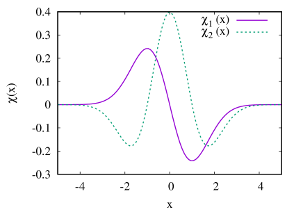
Figure 1: First two wavelets of the Gaussian wavelet family (13)

Their Fourier images are

$$\tilde{\chi}_{n}(k)=-(\imath k)^{n}e^{-\frac{k^{2}}{2}}.$$ (14)

Respectively, the normalization constants and the wavelet cutoff functions are:

$$C_{\chi_{n}}=\frac{\Gamma(n)}{2},\quad f_{\chi_{n}}(x)=\frac{\Gamma(n,x^{2})}{\Gamma(n)},$$

where $\Gamma(\cdot)$ is the Euler gamma function, and $\Gamma(\cdot,\cdot)$ is the incomplete gamma function. For the first two wavelets the wavelet cutoff functions are:

$$f_{\chi_{1}}(x)=e^{-x^{2}},\quad f_{\chi_{2}}(x)=(1+x^{2})e^{-x^{2}}.$$ (15)

We will now proceed to the calculation of one-loop diagrams in wavelet-based Euclidean QED. These are the vacuum polarization diagram and the fermion self-energy diagram, shown in Figs. 2,3.

Vacuum polarization diagram.

First we calculate the vacuum polarization diagram shown in Fig. 2.

Figure 2: Vacuum polarization diagram in scale-dependent QED

For the convenience of calculations, we symmetrize the loop momenta. The external lines of the diagram are labelled by scale arguments $a$ and $a^{\prime}$. So, according to the assumptions made above, the integration in scale arguments in the fermion loop is limited from below by the minimal scale $\mathcal{A}=\min(a,a^{\prime})$. In contrast to the paper Altaisky and Kaputkina (2013a), intended for calculation of the Green functions of scale-dependent fields $\langle\psi_{a_{1}}(x_{1})\ldots\psi_{a_{n}}(x_{n})\rangle$, here we do not specify any propagators on external lines so that the results can be taken as usual diagrams regularized to a scale $\mathcal{A}$. That is why the wavelet factors are omitted in the definitions of 1PI diagrams. Doing so, we get the expression for the vacuum polarization diagram:

$$\Pi_{\mu\nu}^{(\mathcal{A})}(p) = -e^{2}\int\frac{\mathrm{Sp}(\gamma_{\mu}(\not{q}+\frac{\not{p}}{2}-m)\gamma_{\nu}(\not{q}-\frac{\not{p}}{2}-m))}{\left[(q+\frac{p}{2})^{2}+m^{2}\right]\left[(q-\frac{p}{2})^{2}+m^{2}\right]}F_{\mathcal{A}}(p,q)\frac{d^{4}{q}}{(2\pi)^{4}}$$ (16)

$$= -4e^{2}\int\frac{2q_{\mu}q_{\nu}-\frac{1}{2}p_{\mu}p_{\nu}+\delta_{\mu\nu}(\frac{p^{2}}{4}-q^{2}-m^{2})}{\left[(q+\frac{p}{2})^{2}+m^{2}\right]\left[(q-\frac{p}{2})^{2}+m^{2}\right]}F_{\mathcal{A}}(p,q)\frac{d^{4}{q}}{(2\pi)^{4}}.$$

Here we use the function $Sp()$ to denote the trace of the Dirac gamma matrices. The wavelet cutoff function $F_{\mathcal{A}}(p,q)$ is the product of wavelet cutoff functions of the loop momenta:

$$F_{\mathcal{A}}(p,q)=f^{2}\left(\mathcal{A}\left(\frac{p}{2}-q\right)\right)f^{2}\left(\mathcal{A}\left(\frac{p}{2}+q\right)\right).$$ (17)

Let us start the calculations with $\chi_{1}$ wavelet. In this case (Eq.(15)):

$$F_{\mathcal{A}}(p,q)=e^{-\mathcal{A}^{2}p^{2}-4\mathcal{A}^{2}q^{2}},$$

and we have the integral

$$\Pi_{\mu\nu}^{(\mathcal{A},\chi_{1})} = -\frac{e^{2}p^{2}}{\pi^{3}}e^{-\mathcal{A}^{2}p^{2}}\int_{0}^{\infty}dyye^{-4\mathcal{A}^{2}p^{2}y^{2}}\int_{0}^{\pi}d\theta\sin^{2}\theta\times$$

$$\times \frac{2y_{\mu}y_{\nu}-\frac{1}{2}\frac{p_{\mu}p_{\nu}}{p^{2}}+\delta_{\mu\nu}(\frac{1}{4}-y^{2}-\frac{m^{2}}{p^{2}})}{\left[\frac{\frac{1}{4}+y^{2}+\frac{m^{2}}{p^{2}}}{y}+\cos\theta\right]\left[\frac{\frac{1}{4}+y^{2}+\frac{m^{2}}{p^{2}}}{y}-\cos\theta\right]},$$ (18)

where we have introduced a dimensionless vector $y$ in the direction of loop momentum: $q=|p|y$, with $\theta$ being the angle between $p$ and $q$. The integral (18) can be evaluated analytically in relativistic limit $p^{2}\gg 4m^{2}$. This gives:

$$\Pi_{\mu\nu} =I_{T}\left(\delta_{\mu\nu}-\frac{p_{\mu}p_{\nu}}{p^{2}}\right)+I_{L}\frac{p_{\mu}p_{\nu}}{p^{2}},$$ (19)

$$I_{T} =\frac{e^{2}p^{2}}{48\pi^{2}s^{3}}\Bigl{[}(4s^{2}-2s-1)e^{-2s}+(1+s-4s^{2})e^{-s}$$

$$+4s^{3}(\mathrm{Ei}_{1}(s)-2\mathrm{Ei}_{1}(2s))\Bigr{]},$$

$$I_{L} =\frac{e^{2}p^{2}}{16\pi^{2}s^{3}}e^{-2s}\left((s-1)e^{s}+1\right),$$

where $s\equiv\mathcal{A}^{2}p^{2}$ is dimensionless scale argument, $\mathrm{Ei}_{1}(z)=\int_{1}^{\infty}\frac{e^{-xz}}{x}dx$ is exponential integral of the first type. The details of the calculations are presented in the Appendix. As we can see from Eqs.(59,60), the longitudinal part of $\Pi_{\mu\nu}$ does not vanish in the limit of $s\to 0$. In this sense, the wavelet observation scale $\mathcal{A}$ plays the role of inverse regularising mass $\frac{1}{M}$ of the Pauli-Villars regularization Bogoliubov and Shirkov (1980). In contrast to dimensional regularization, where $q_{\mu}q_{\nu}$ and $2q^{2}$ terms cancel each other in the sense of leading divergences, this does not happen in the theory with a finite scale $\mathcal{A}$ and local gauge invariance. There may be different reasons for that. First, the finite terms, neglected by dimensional regularization turn into the scale-dependent contributions, which can’t be neglected in our case. Second, the scale $\mathcal{A}$ is a scale in Euclidean space and we cannot match it exactly to what is measured in Minkowski space. Third, changing the coordinates from $\mathbf{x}$ to $(\mathbf{x},a)$ we need to pay an extra attention on what is gauge invariance in scale-dependent settings Altaisky (2020) – the consideration presented above ignored this completely by making standard assumption of local gauge invariance.

Fermion self- diagram.

The loop integral of the fermion self-energy diagram, shown in Fig. 3, has the form:

$$\Sigma^{(\mathcal{A})}(p)=-\imath e^{2}\int\frac{d^{4}{q}}{(2\pi)^{4}}\frac{F_{\mathcal{A}}(p,q)\gamma_{\mu}\left[\frac{\not{p}}{2}-\not{q}-m\right]\gamma_{\mu}}{\left[\left(\frac{p}{2}-q\right)^{2}+m^{2}\right]\left[\frac{p}{2}+q\right]^{2}}.$$ (20)

As in the previous example, $A$ is the minimal scale of all external lines $\mathcal{A}=\min(a,a^{\prime})$.

Figure 3: Fermion self-energy diagram in scale-dependent QED

We will calculate the diagram (20) with the wavelet-cutoff functions $F_{\mathcal{A}}(p,q)$ for both $\chi_{1}$ and $\chi_{2}$ wavelets (15).

Using the identities for Euclidean gamma matrices, and assuming the relativistic limit $p^{2}\gg 4m^{2}$ for simplicity of calculations, we rewrite (20) in the form

$$\Sigma^{(\mathcal{A})}(p)=-\imath e^{2}\int\frac{d^{4}{y}}{(2\pi)^{4}}F_{\mathcal{A}}(p,|p|y)\frac{(\not{p}+4m-2|p|\not{y})}{\left[y^{2}+\frac{1}{4}-y\cos\theta-\frac{m^{2}}{p^{2}}\right]\left[y^{2}+\frac{1}{4}+y\cos\theta\right]},$$ (21)

where the term proportional to $\not{y}$ in the numerator can be ignored, if we make the denominator symmetric with respect to the inversions by omitting the mass term in fermion propagator. For the same reason of relativistic approximation $p^{2}\gg 4m^{2}$, we can regard the mass term in the numerator as negligible in comparison to $\not{p}$.

Under the above-made assumptions, taking the wavelet cutoff function of the type $\chi_{1}$, (Eq.15), we can easily see that

$$\Sigma^{(\mathcal{A})}_{\chi_{1}}(p)=-\frac{\imath e^{2}\not{p}e^{-s}}{16\pi^{4}}\int\frac{dyye^{-4sy^{2}}\sin^{2}\theta d\theta}{\left(y+\frac{1}{4y}\right)^{2}-\cos^{2}\theta}=-\frac{\imath e^{2}e^{-s}}{4\pi^{3}}J\not{p},$$

where the integral $J$ is given by (54). Thus we get:

$$\Sigma^{(\mathcal{A})}_{\chi_{1}}(p)=-\frac{\imath e^{2}}{16\pi^{2}}\left[2\mathrm{Ei}_{1}(2s)-\mathrm{Ei}_{1}(s)-\frac{e^{-2s}}{s}+\frac{e^{-s}}{s}\right]\not{p}.$$ (22)

Fermion-photon vertex.

The one-loop contribution to the fermion-photon vertex is shown in Fig. 4.

Figure 4: One-loop contribution to the fermion-photon vertex in QED. $p_{1}+p_{2}+p_{3}=0$.

Since the bare fermion-photon vertex is $-\imath e\gamma_{\rho}$, we similarly normalize the vertex function:

$$-\imath e\Gamma_{\rho}^{(\mathcal{A})}(p_{1},p_{2},p_{3})=-\imath e\gamma_{\rho}+(-\imath e)^{3}\int\frac{d^{4}l}{(2\pi)^{4}}\frac{\gamma_{\mu}\imath(\not{l}_{2}+m)\gamma_{\rho}\imath(\not{l}_{1}+m)\gamma_{\mu}}{(l_{2}^{2}+m^{2})(l_{1}^{2}+m^{2})l_{3}^{2}}f^{2}(\mathcal{A}l_{1})f^{2}(\mathcal{A}l_{2})f^{2}(\mathcal{A}l_{3}),$$ (23)

where $f(x)$ is the wavelet-cutoff function given by (12). To get rid of the angle dependence in the wavelet cutoff factors we have symmetrized the loop momenta:

$$l_{1}=l+\frac{p_{3}-p_{2}}{3},\quad l_{2}=l+\frac{p_{1}-p_{3}}{3},\quad l_{3}=l+\frac{p_{2}-p_{1}}{3}.$$

To calculate the one-loop contribution to the vertex let us consider the decay of a photon with momentum $p_{3}=p$ into a fermion-antifermion pair. This corresponds to the loop momenta

$$l_{1}=l+\frac{p}{2},\quad l_{2}=l-\frac{p}{2},\quad l_{3}=l.$$ (24)

Considering the relativistic case $p^{2}\gg 4m^{2}$ we can omit the mass terms. This gives

$$A_{\rho} =\gamma_{\mu}\left(\not{l}-\frac{\not{p}}{2}\right)\gamma_{\rho}\left(\not{l}+\frac{\not{p}}{2}\right)\gamma_{\mu}$$

$$=2\left(\not{l}+\frac{\not{p}}{2}\right)\gamma_{\rho}\left(\not{l}-\frac{\not{p}}{2}\right).$$

The one-loop contribution to the vertex then takes the form

$$\Lambda_{\rho}\left(-\frac{p}{2},-\frac{p}{2},p\right)=-e^{2}\int\frac{d^{4}l}{(2\pi)^{4}}\frac{A_{\rho}F_{\mathcal{A}}(p,l)}{\left(l-\frac{p}{2}\right)^{2}\left(l+\frac{p}{2}\right)^{2}l^{2}}.$$ (25)

The vertex wavelet cutoff factor is the product of three wavelet cutoff functions:

$$F_{\mathcal{A}}(p,l)=f^{2}\left(\mathcal{A}\left(l-\frac{p}{2}\right)\right)f^{2}\left(\mathcal{A}\left(l+\frac{p}{2}\right)\right)f^{2}(\mathcal{A}l).$$ (26)

For the case of $\chi_{1}$ wavelet, see Eq. 15, we have

$$F_{\mathcal{A}}(p,l)=\exp\left(-\mathcal{A}^{2}p^{2}-6\mathcal{A}^{2}l^{2}\right).$$

The calculation of the integral (25) with this cutoff function, presented in Appendix, gives:

$$\Lambda_{\rho}\left(-\frac{p}{2},-\frac{p}{2},p\right)=\frac{e^{2}\gamma_{\rho}}{3\pi^{2}}\Bigg{[}e^{\frac{s}{2}}\mathrm{Ei}_{1}(3s)-\frac{e^{\frac{s}{2}}\mathrm{Ei}_{1}\left(\frac{3s}{2}\right)}{2}$$

$$-\frac{e^{-\frac{5s}{2}}}{8s}+\frac{e^{-s}}{12s}-\frac{5e^{-s}\mathrm{Ei}_{1}\left(\frac{3s}{2}\right)}{16}+\frac{e^{-s}}{36s^{2}}-\frac{e^{-\frac{5s}{2}}}{36s^{2}}\Bigg{]}.$$ (27)

In terms of the fine structure constant $\alpha(s)=\frac{e^{2}(s)}{4\pi}$ the one-loop contribution to the QED vertex (27) can be cast in the form

$$\alpha(s) =\alpha\left[1+\frac{4}{3\pi}\alpha R(s)\right]^{2},$$ (28)

$$R(s) =e^{\frac{s}{2}}\mathrm{Ei}_{1}(3s)-\frac{e^{\frac{s}{2}}\mathrm{Ei}_{1}\left(\frac{3s}{2}\right)}{2}-\frac{e^{-\frac{5s}{2}}}{8s}+$$

$$+\frac{e^{-s}}{12s}-\frac{5e^{-s}\mathrm{Ei}_{1}\left(\frac{3s}{2}\right)}{16}+\frac{e^{-s}}{36s^{2}}-\frac{e^{-\frac{5s}{2}}}{36s^{2}}.$$ (29)

The graph of the running coupling constant $\alpha(s)$, calculated according to the formula (28), is shown in Fig. 5 below.

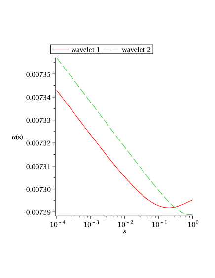
Figure 5: Running coupling constant calculated for both wavelets $\chi_{1}$ and $\chi_{2}$ according to the formula (28). The value of the fine structure constant is $\alpha_{\infty}=1/137.036$.

Decomposing Eq.(27) in a series for small scales ($s\to 0$)

$$\Lambda_{\rho}\approx\gamma_{\rho}e^{2}\frac{\frac{3}{2}-\frac{9}{16}\gamma+\frac{13}{16}\ln\frac{3}{2}-\frac{3}{16}\ln s-\ln 3}{3\pi^{2}}+O(s),$$

we get the logarithmic derivative

$$\frac{\partial e(s)}{\partial\ln s}=-\frac{e^{3}}{16\pi^{2}}.$$ (30)

The calculations performed with $\chi_{2}$ wavelet, presented in Appendix, give similar results.

III Ward identities

Formally, the Ward-Takahashi identities follow from a requirement that the Green function generating functional, designed on an action $S[\phi]$, should be invariant under the the same symmetry transformations $\phi(x)\to\phi(x)+\delta\phi(x)$ that leave the action invariant. For the case of spinor electrodynamics, the infinitesimal gauge transformations $\delta\phi$ take the form:

$$\delta A_{\mu}=\partial_{\mu}\Lambda(x),\quad\delta\psi=-\imath e\Lambda(x)\psi,\quad\delta\bar{\psi}=\imath e\Lambda(x)\bar{\psi}.$$

Since the Lagrangian is gauge-invariant by construction, to make the generation functional $Z[J,\bar{\eta},\eta]$ gauge invariant, we need to ensure that the variations of the source terms and the gauge-fixing terms compensate each other. This implies

$$\int\mathcal{D}A\mathcal{D}\bar{\psi}\mathcal{D}\psi\left[e^{-\int d^{4}x(L_{E}+J_{\mu}A_{\mu}+\imath\bar{\eta}\psi+\imath\bar{\psi}\eta)}e^{\delta_{\Lambda}}\right]=$$

$$=\int\mathcal{D}A\mathcal{D}\bar{\psi}\mathcal{D}\psi e^{-\int d^{4}x(L_{E}+J_{\mu}A_{\mu}+\imath\bar{\eta}\psi+\imath\bar{\psi}\eta)},$$

where

$$\delta_{\Lambda}\equiv\int d^{4}x\left[-\frac{1}{\alpha}\partial^{2}(\partial_{\mu}A_{\mu})+\partial_{\mu}J_{\mu}+e(\bar{\psi}\eta-\bar{\eta}\psi)\right]\Lambda(x).$$ (31)

Considering an infinitesimal transform we can approximate $e^{\delta_{\Lambda}}\approx 1+\delta_{\Lambda}$, and hence, in view of arbitrariness of $\Lambda(x)$, the equality $\langle\delta_{\Lambda}\rangle=0$ can be written in a form of variational equation:

$$\bigl{[}-\frac{1}{\alpha}\partial^{2}(\partial_{\mu}A_{\mu})+\partial_{\mu}J_{\mu}+e(\bar{\psi}\eta-\bar{\eta}\psi)\bigr{]}Z[J,\bar{\eta},\eta]=0,$$ (32)

$$\hbox{where\ }\psi(x)=\imath\frac{\delta}{\delta\bar{\eta}(x)},\bar{\psi(x)}=\imath\frac{\delta}{\delta\eta(x)},A_{\mu}=-\frac{\delta}{\delta J_{\mu}(x)}.$$

The Ward-Takahashi identities can be obtained by taking an appropriate number of functional derivatives of the equation (32). This is usually done by changing from the generating functional $Z$ to the generating functional for the connected Green’s functions:

$$Z[J,\bar{\eta},\eta]=e^{-W[J,\bar{\eta},\eta]},$$

and then applying the Legendre transform to get an effective action functional:

$$\Gamma[A,\psi,\bar{\psi}]=W[J,\bar{\eta},\eta]-JA-\imath\bar{\eta}\psi-\imath\bar{\psi}\eta.$$

The latter enables us to work with proper vertices and write the Ward-Takahashi identities generating equation in the form:

$$\frac{\partial^{2}}{\alpha}\partial_{\mu}A_{\mu}+\partial_{\mu}\frac{\delta\Gamma}{\delta A_{\mu}}+\imath e\left(\psi\frac{\delta\Gamma}{\delta\psi}-\bar{\psi}\frac{\delta\Gamma}{\delta\bar{\psi}}\right)=0.$$ (33)

The first derivative of (33) with respect to $A_{\mu}$ gives the Ward identity Ward (1950) that demands the transversality of the vacuum polarization diagram:

$$\partial_{\mu}\Pi_{\mu\nu}=0.$$ (34)

The integrals in the vacuum polarization diagram will satisfy the requirement (34) only in case they are invariant under the shift of the loop momenta. This is not always true when a regularization procedure is applied. In QED, the condition (34) is observed by dimensional regularization, but not by the momentum cutoff. That is why dimensional regularization has become the most common regularization method in QFT models ’t Hooft and Veltman (1972).

To fulfil the Ward-Takahashi identities, a regulator is usually assumed to satisfy the requirement of the type Battistel and Nemes (1999); Cynolter and Lendvai (2011):

$$\int\frac{d^{4}l}{(2\pi)^{4}}\frac{l_{\mu}l_{\nu}}{(l^{2}+\Delta)^{2}}=\frac{\delta_{\mu\nu}}{2}\int\frac{d^{4}l}{(2\pi)^{4}}\frac{1}{l^{2}+\Delta}$$ (35)

(the integration over the Feynman $x$-parameter used to get rid of angle integrations is not shown here). This is definitely true for dimensional regularization, but is not true for momentum-cutoff and is not true for the wavelet regularization we consider in this paper. In our case of finite theory we cannot use a relation like (35) as a ”rule”, but have to evaluate everything explicitly.

Regardless of the undoubted merits of dimensional regularization, it deals only with the main singular parts of Feynman diagrams, and cannot tackle the amplitudes at finite scales. In this respect, the finite cutoff regularization and the wavelet regularization have the potential advantage of describing of what happens at a finite observation scale Gu (2002); Altaisky (2010). The goal of the wavelet-cutoff technique, provided by continuous wavelet transform, is to get a capability of calculations at finite observation scale. The respect to the gauge invariance can be also imposed in a cutoff-momentum regularization scheme by assuming the gauge transformations to act below the momentum cutoff $\Lambda$ Gu (2006):

$$a_{\mu}(k)\to a_{\mu}(k)-\imath k_{\mu}\lambda(k),\quad\hbox{with\ }\lambda(|k|>\Lambda)=0.$$ (36)

In the case of continuous wavelet transform regularization, there is an alternative – to consider gauge transformations which directly depend on the scale argument $a$ :

$$\psi_{a}(x)\to e^{-\alpha_{a}(x)}\psi_{a}(x)$$ (37)

Doing so, we get a theory that is gauge invariant separately at each given scale Altaisky (2020).

We do not consider scale-dependent modifications of gauge invariance in this paper, leaving this subject for future studies. Instead, the above considered wavelet cutoff factors of Gaussian type, are rather similar to already proposed exponential modifications of the momentum cutoff Oleszczuk (1994), based on the Schwinger proper time method Schwinger (1951). Using wavelet regularization, in the case of small scales $s\ll 1$, when in the final limit of $s\to 0$ the integration over all scales $\int_{0}^{\infty}\frac{da}{a}$ would definitely restore the symmetries of the original theory, we can use the approximation formulae that follow from Ward identities of the full (non-regularized) theory.

Technically, the Ward identities follow from the observation that a proper vertex of the fermion-photon interaction can be associated with the fermion self-energy diagram by inserting a photon line in the internal fermion line of the latter. Ward noticed, that for the bare inverse electron propagator

$$S_{(e)}^{-1}(p)=\imath(\not{p}+m),$$

the derivative with respect to the momentum $p_{\mu}$ gives the fermion-photon interaction vertex:

$$\frac{\partial S_{(e)}^{-1}(p)}{\partial p_{\mu}}=\imath\gamma_{\mu}.$$

He proved the same for the inverse full propagator:

$$\frac{\partial G_{(e)}^{-1}(p)}{\partial p_{\mu}}=\imath\Gamma_{\mu},$$ (38)

where $-\imath e\gamma_{\mu}$ and $-\imath e\Gamma_{\mu}$ are the bare and the full vertex of the fermion-photon interaction. (Here we use the Euclidean notation, in contrast to the original paper of Ward Ward (1950), written in Minkowski space.)

More generally, the Ward-Takahashi Takahashi (1957) identity in spinor electrodynamics, written in integral form, relates the vertex function to the difference of fermion propagators:

$$q_{\mu}\Gamma_{\mu}(p,-p-q,q)=G^{-1}(p+q)-G^{-1}(p).$$ (39)

Here $G(p)$ is the full fermion propagator. The identity (39) is a helpful constraint which ensures the gauge invariance of the renormalized QED in any order of perturbation theory Ward (1950); Takahashi (1957). The constraint (39) makes the perturbation expansion gauge-invariant at the presence of the gauge fixing terms in the QED generating functional.

The most direct application of Ward’s finding is the calculation of the full fermion-photon vertex in the limit of zero photon momentum. In this case:

$$\Gamma_{\mu}(p,-p,0)=\gamma_{\mu}+\Lambda_{\mu}(p,-p,0).$$ (40)

As it follows from the Dyson equation, the inverse full propagator is equal to

$$G^{-1}(p)=S^{-1}(p)-\Sigma(p),$$ (41)

where $\Sigma(p)$ is the electron self-energy. Taking the derivatives of both sides of (41) by $\frac{\partial}{\partial p_{\mu}}$ we get

$$\Lambda_{\mu}(p,-p,0)=\imath\frac{\partial\Sigma(p)}{\partial p_{\mu}}.$$ (42)

The formula (42) can now be applied to our wavelet-regularized calculations of one-loop diagrams. Since we are interested only in the contributions to the vertex, proportional to $-\imath e\gamma_{\mu}$, it is sufficient to differentiate only the last multiplier in (22): $\frac{\partial\not{p}}{\partial p_{\mu}}=\gamma_{\mu}$. This gives the one-loop equation for the fermion-photon vertex regularized at scale $\mathcal{A}$:

$$-\imath e\Gamma^{(\mathcal{A})}_{\chi_{1},\mu}(p) = -\imath e\gamma_{\mu}\left[1+\frac{e^{2}}{16\pi^{2}}R_{1}^{\chi_{1}}(s)\right]+\ldots,$$

$$R_{1}^{\chi_{1}}(s) \equiv 2\mathrm{Ei}_{1}(2s)-\mathrm{Ei}_{1}(s)-\frac{e^{-2s}}{s}+\frac{e^{-s}}{s}.$$ (43)

Since whole dependence on the scale in our model is contained in function $R_{1}(s)$, we can now calculate the dependence on the scale of the effective charge. The wavelet regularization scheme includes the integration of over all scale components from observation scale $A$ to infinity. The equation (43) thus gives the value of the effective charge $e_{eff}(s)$, i.e. the effective charge measured at scale $\mathcal{A}$, in terms of physical electron charge measured at infinity $e_{0}=e(\infty)$. It is convenient to rewrite it in terms of the fine structure constant

$$\alpha(s)=\frac{e^{2}(s)}{4\pi},$$

the physical value of which is $\alpha\approx 1/137.036$ Van Dyck et al. (1987); Kinoshita and Nio (2006). Then, the scale dependence of the effective charge, given in one-loop approximation by the equation (43), is:

$$\alpha(s)=\alpha\left(1+\frac{\alpha}{4\pi}R_{1}(s)\right)^{2}.$$ (44)

Since we use the coordinate scale $a$ as the scale argument the sign will be opposite to that in dimensional regularization $s\frac{\partial}{\partial s}\to-\mu^{2}\frac{\partial}{\partial\mu^{2}}$. The scaling equation for the effective charge – we do not call it RG-equation, since there is no field renormalization in our model – takes the form:

$$s\frac{\partial e_{eff}}{\partial s}=\frac{e_{eff}^{3}}{16\pi^{2}}s\frac{\partial R_{1}(s)}{\partial s},$$ (45)

$$s\frac{\partial R_{1}(s)}{\partial s}=\frac{e^{-s}}{s}\left(e^{-s}-1\right).$$

The scaling equation (45) can be integrated in a usual RG-like the form:

$$\frac{de_{eff}}{e_{eff}^{3}}=\frac{ds}{16\pi^{2}}\frac{e^{-s}}{s^{2}}\left(e^{-s}-1\right).$$ (46)

The solution of the equation (46) is given by

$$e_{eff}^{2}(s)=\frac{e_{0}^{2}}{1-\frac{e_{0}^{2}}{8\pi^{2}}R_{1}(s)},$$

which can be cast in terms of the fine structure constant:

$$\alpha(s)=\frac{\alpha}{1-\frac{\alpha}{2\pi}R_{1}(s)}.$$ (47)

Similar results can be obtained using other wavelets. In this way using $\chi_{2}$ wavelet cutoff, see Eq.(71) in Appendix, we get:

$$R_{1}^{\chi_{2}}(p) =2\mathrm{Ei}_{1}(2s)-\mathrm{Ei}_{1}(s)-\frac{e^{-2s}(s+5)}{2s}+$$

$$+\frac{e^{-s}(s^{3}+18s^{2}+134s+640)}{256s}.$$ (48)

The scale dependences of $\alpha(s)$, calculated for both cases of (15) wavelet cutoff functions, are shown in Fig. 6.

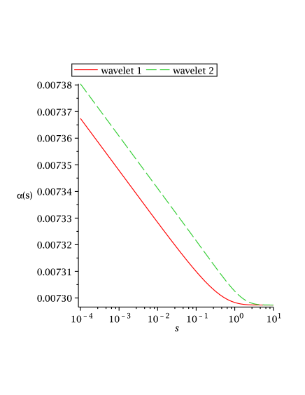
Figure 6: Scale dependence of the fine structure constant $\alpha(s)=\frac{e_{eff}^{2}(s)}{4\pi}$. Two curves correspond to the one-loop approximation (47), performed with $\chi_{1}$ and $\chi_{2}$ wavelet cutoff, respectively.

.

Since the value of $\alpha$ is small, the value of $\alpha(s)$ given by Eq.(47) is practically indistinguishable from that given by (43). The Landau singularity in Eq.(47) matters only when $s\sim e^{-\frac{2\pi}{\alpha}}$, so that

$$\frac{2\pi}{\alpha}\approx R_{1}(s)=1-\gamma-2\ln 2-\ln s+\frac{3}{2}s+O(s^{2}),$$ (49)

with $\gamma\approx 0.5772$ being the Euler-Mascheroni constant.

IV Conclusions

The basic symmetries of quantum electrodynamics are the relativistic invariance and the gauge invariance. In the standard approach to QED, which assumes the quantum fields to be local square-integrable functions, the calculations of observable quantities may violate both the Lorentz symmetry and the gauge symmetry due to the formal infinities of the calculated Green functions. Different regularization schemes have been used to get rid of divergences. The momentum cutoff regularization was historically the first. In low-energy effective theories there is a natural cutoff momentum $\Lambda$, above which the theory loses its validity. However, this cannot be applied considering a fundamental theory rather than effective theory. The dimensional regularization has become the most common, utmost a standard way of regularization, because it does not violate the gauge symmetry; although it is not ubiquitous being incapable of treating supersymmetric theories Stöckinger (2005).

Wavelet regularization is different from all above mentioned regularizations. It changes the space of functions from the space of square-integrable functions to the space of functions $\psi_{a}(x)$, depending on both the coordinate $x$, and the scale $a$. The former is dynamical – it enters the dynamical equations, the latter describes only the settings of observations and does not enter any dynamical equations. In this sense, we extend the description of observed physical fields by incorporating the conditions of observation ($a,\chi$) in the field definition. A physical field per se is then a collection of all physical fields that can be potentially observed: $\Psi=\{\psi_{a}(x,\cdot)\}_{a,\chi,\ldots}$. It cannot keep the perturbation expansion locally gauge invariant. Since the scale-dependent fields are defined not in a sharp point $x$, but in a region of typical size $a$, there is no need of infinite momentum injection to measure such fields, and there are no physical reasons for the appearing of UV divergences.

The key issue of the theory of scale-dependent fields is the problem of how the physical particles interact with each other. The description of physical interactions is determined by the symmetry of the problem. In this way, the symmetry with respect to local $U(1)$ transformations determines electromagnetic interaction, the symmetry with respect to $SU(3)$ gauge transformations determines the strong interactions, and so on. In the present paper, we have followed exactly the same way: electrodynamics is understood as a theory with $U(1)$ gauge group, acting on the space of square-integrable local functions. This definition immediately implies that the physically observed fields $\psi_{a}(x)$ are merely projections of square-integrable fields $\psi(x)$ performed with the help of a mother wavelet $\chi$. This is a rather strong restriction: it states that gauge interactions take place in the space of local square-integrable functions and inverse wavelet transform is used to reconstruct the local fields from a set of their projections; the interaction then takes place between the reconstructed fields. In this sense, wavelet regularization is similar to momentum cutoff regularization and gives the dependence of physical parameters on the observation scale.

Having performed the calculations, presented in this paper, we have found out that wavelet regularization can give a qualitatively adequate description of the QED running coupling constant (in one-loop approximation), which increases with the logarithm of the inverse observation scale. The advantage of wavelet regularization, if compared to dimensional regularization and other methods, is that it does not need any external tools, such as renormalization, which is always demanded by dimensional regularization to get physically interpretable results. The reason is that the wavelet transform itself is already based on the group of scale transformations, similar to the renormalization group. That is why instead of the renormalization group equations we have just a logarithmic derivative of the effective charge with respect to the dimensionless scale argument $s$. This $s=(\mathcal{A}p)^{2}$ is similar to the normalization scale $1/\mu^{2}$ in dimensional regularization but has a physical interpretation in terms of the measurement scale. The crucial difference from standard renormalization group approach is that we face no divergences to get rid of and we have no field renormalization. The latter is due to the fact that by extending the space of fields $\psi(x)$ to the space of scale-dependent fields $\psi_{a}(x)$ we already get the collections of all scales rather than a poor man collection of two scales only. At the same time, our calculations show that known results such as Landau pole of the form $\frac{1}{1-\alpha X}$ also take place in a wavelet theory finite by construction, but in the latter case they have a more mild form of $1+\alpha X$, where $\alpha X$ is small and there is no threat of a pole.

At the same time, we have to admit that our persistence on keeping the standard definition of gauge invariance in the space of local field does not allow to preserve the transversality of the vacuum polarization operator at the one-loop level: $p_{\mu}\Pi_{\mu\nu}(p)\neq 0$. This has long been known for the momentum-cutoff and other regularization schemes and is quite expected for the wavelet regularization of a locally defined gauge theory: having declared the scale-dependent fields to be the physically observed fields we still insist that gauge interaction acts on local fields. It might be more reasonable do define the interaction directly in the space of scale-dependent fields, as is proposed in Altaisky (2020) in the context of QCD, but this is planned for future research.

Appendix A Calculations with $\chi_{1}$ wavelet

A.1 Vacuum polarization diagram

Substituting the integration measure $d^{4}q=4\pi q^{3}dq\sin^{2}\theta d\theta$ into the integral (16) and dividing both the numerator and the denominator by $p^{2}q^{2}$ we arrive at the equation (18):

$$\Pi_{\mu\nu}^{(\mathcal{A},\chi_{1})}=-\frac{e^{2}p^{2}}{\pi^{3}}e^{-\mathcal{A}^{2}p^{2}}\int_{0}^{\infty}dyye^{-4\mathcal{A}^{2}p^{2}y^{2}}\int_{0}^{\pi}d\theta\sin^{2}\theta\frac{2y_{\mu}y_{\nu}-\frac{1}{2}\frac{p_{\mu}p_{\nu}}{p^{2}}+\delta_{\mu\nu}(\frac{1}{4}-y^{2}-\frac{m^{2}}{p^{2}})}{\left[\frac{\frac{1}{4}+y^{2}+\frac{m^{2}}{p^{2}}}{y}+\cos\theta\right]\left[\frac{\frac{1}{4}+y^{2}+\frac{m^{2}}{p^{2}}}{y}-\cos\theta\right]}.$$

The angle part of integral (18) can be evaluated explicitly. The corresponding integrals have the form:

$$I_{k}[\beta(y)]=\int_{0}^{\pi}d\theta\frac{\sin^{2}\theta\cos^{2k}\theta}{\beta^{2}-\cos^{2}\theta},\quad I_{0}[\beta(y)]=\pi(1-\sqrt{1-\beta^{-2}}),\quad I_{1}[\beta(y)]=-\frac{\pi}{2}+\beta^{2}I_{0}[\beta],$$ (50)

where in our case $\beta$ depends on $y$. To make the calculations analytically feasible, we simplify the matter by considering the relativistic limit $p^{2}\gg 4m^{2}$. In this limit

$$\beta(y)=y+\frac{1}{4y}.$$ (51)

In this approximation the vacuum polarization integral takes the form

$$\Pi_{\mu\nu}^{(\mathcal{A},\chi_{1})}=-\frac{e^{2}p^{2}}{\pi^{3}}e^{-\mathcal{A}^{2}p^{2}}\int_{0}^{\infty}dyye^{-4\mathcal{A}^{2}p^{2}y^{2}}\int_{0}^{\pi}d\theta\sin^{2}\theta\frac{2y_{\mu}y_{\nu}-\frac{1}{2}\frac{p_{\mu}p_{\nu}}{p^{2}}+\delta_{\mu\nu}(\frac{1}{4}-y^{2})}{\beta^{2}(y)-\cos^{2}\theta}.$$

There are two basic integrals here: the scalar integrals, which do not contain $y_{\mu}y_{\nu}$, and the tensor integrals, which contain these terms. The scalar integral has the form:

$$J\equiv\int_{0}^{\infty}dyye^{-4sy^{2}}I_{0}[\beta(y)].$$ (52)

As it follows from Eqs.(50,51):

$$I_{0}[\beta(y)]=\begin{cases}\frac{8\pi y^{2}}{1+4y^{2}},&0\leq y\leq\frac{1}{2}\cr\frac{2\pi}{1+4y^{2}},&y\geq\frac{1}{2}\end{cases},\qquad I_{1}[\beta(y)]=\begin{cases}2\pi y^{2},&0\leq y\leq\frac{1}{2}\cr\frac{\pi}{8y^{2}},&y\geq\frac{1}{2}\end{cases},$$ (53)

and hence

$$J=8\pi\int_{0}^{\frac{1}{2}}\frac{dyy^{3}e^{-4sy^{2}}}{1+4y^{2}}+2\pi\int_{\frac{1}{2}}^{\infty}\frac{dyye^{-4sy^{2}}}{1+4y^{2}}=\frac{\pi}{4}\left[2\mathrm{Ei}_{1}(2s)e^{s}-\mathrm{Ei}_{1}(s)e^{s}-\frac{e^{-s}}{s}+\frac{1}{s}.\right].$$ (54)

The other scalar integral is a derivative of $J$:

$$I_{q}^{0}=\int_{0}^{\infty}dyy^{3}I_{0}[\beta(y)]e^{-4sy^{2}}=-\frac{1}{4}\frac{dJ}{ds}=-\frac{\pi}{16}\left[2\mathrm{Ei}_{1}(2s)e^{s}-\mathrm{Ei}_{1}(s)e^{s}-\frac{e^{-s}-1}{s}+\frac{e^{-s}-1}{s^{2}}\right].$$

The terms of the integral, which contain $y_{\mu}y_{\nu}$, and which do not, can be evaluated separately. Since our problem has only one preferable direction – the direction of vector $\mathbf{p}$, we can evaluate the tensor integral

$$I^{(2)}_{q\mu\nu}=\int ydy\sin^{2}\theta d\theta e^{-4sy^{2}}\frac{y_{\mu}y_{\nu}}{\left(y+\frac{1}{4y}\right)^{2}-\cos^{2}\theta}$$ (55)

by substituting $y_{\mu}y_{\nu}\to By^{2}\delta_{\mu\nu}+Cy^{2}\frac{p_{\mu}p_{\nu}}{p^{2}}$ in the integrand; where $B$ and $C$ are the constants to be determined.

The integral to be evaluated takes the form

$$I_{\mu\nu}=\int ydy\sin^{2}\theta d\theta e^{-4sy^{2}}\frac{By^{2}\delta_{\mu\nu}+Cy^{2}\frac{p_{\mu}p_{\nu}}{p^{2}}}{\left(y+\frac{1}{4y}\right)^{2}-\cos^{2}\theta}.$$ (56)

The constants $B$ and $C$ are determined from a system of two linear equation

$$\mathrm{Tr}I^{(2)}_{q\mu\nu}=\mathrm{Tr}I_{\mu\nu},\quad I^{(2)}_{q\mu\nu}p_{\mu}p_{\nu}=I_{\mu\nu}p_{\mu}p_{\nu}\qquad\Leftrightarrow 4B+C=1,\quad I_{q}^{1}=(B+C)I_{q}^{0},$$

where

$$I_{q}^{1}=\int_{0}^{\infty}y^{3}dye^{-4sy^{2}}I_{1}[\beta(y)]=\frac{\pi}{32}\frac{e^{-s}}{s^{3}}\left[e^{s}-s-1\right].$$

Hence we can determine the constants $B$ and $C$ in terms of $\eta\equiv\frac{I_{q}^{1}}{I_{q}^{0}}$:

$$B=\frac{1-\eta}{3},\quad C=\frac{4\eta-1}{3},\qquad\eta=\frac{1}{2}\frac{1+s-e^{-s}}{s^{3}e^{2s}(2\mathrm{Ei}_{1}(2s)-\mathrm{Ei}_{1}(s))+s(s-1)(e^{s}-1)},$$

and now can evaluate the vacuum polarization diagram

$$\Pi_{\mu\nu} =-\frac{e^{2}p^{2}}{\pi^{3}}e^{-s}\left(I_{q}+I_{p}+I_{t}\right)\equiv I_{T}\delta_{\mu\nu}+I_{P}\frac{p_{\mu}p_{\nu}}{p^{2}},$$ (57)

$$I_{t} =\frac{1}{2}\left(\delta_{\mu\nu}-\frac{p_{\mu}p_{\nu}}{p^{2}}\right)J,\qquad I_{p}=-\frac{\delta_{\mu\nu}}{4}J,\quad I_{q}=2I^{(2)}_{q\mu\nu}-\delta_{\mu\nu}I^{0}_{q}=\left[\delta_{\mu\nu}(2B-1)+2C\frac{p_{\mu}p_{\nu}}{p^{2}}\right]I^{0}_{q},$$

$$I_{T} =-\frac{e^{2}p^{2}}{\pi^{3}}e^{-s}\left[(2B-1)I_{q}^{0}+\frac{J}{4}\right],\quad I_{P}=-\frac{e^{2}p^{2}}{\pi^{3}}e^{-s}\left[2CI_{q}^{0}-\frac{J}{2}\right].$$ (58)

After simple algebra, we get the final expressions:

$$I_{T} =\frac{e^{2}p^{2}}{48\pi^{2}s^{3}}\Bigl{[}(4s^{2}-2s-1)e^{-2s}+(1+s-4s^{2})e^{-s}+4s^{3}(\mathrm{Ei}_{1}(s)-2\mathrm{Ei}_{1}(2s))\Bigr{]}$$ (59)

$$I_{P} =\frac{e^{2}p^{2}}{48\pi^{2}s^{3}}\Bigl{[}(-4s^{2}+2s+4)e^{-2s}+2(2s^{2}+s-2)e^{-s}-4s^{3}(\mathrm{Ei}_{1}(s)-2\mathrm{Ei}_{1}(2s))\Bigr{]},$$ (60)

$$I_{L} =I_{T}+I_{P}=\frac{e^{2}p^{2}}{16\pi^{2}s^{3}}e^{-2s}\left((s-1)e^{s}+1\right).$$

We can represent the vacuum polarization diagram is a standard form:

$$\Pi_{\mu\nu} =I_{T}\left(\delta_{\mu\nu}-\frac{p_{\mu}p_{\nu}}{p^{2}}\right)+I_{L}\frac{p_{\mu}p_{\nu}}{p^{2}}.$$

A.2 One-loop corrections to the QED vertex calculated with $\chi_{1}$ wavelet cutoff

To evaluate the integral (25) we take the tensor structure in the form

$$A_{\rho}=2\not{l}\gamma_{\rho}\not{l}-\frac{1}{2}\not{p}\gamma_{\rho}\not{p},$$

omitting the terms linear in $l$ and using the massless limit. Thus the whole integral in (25) takes the form:

$$I_{\triangle}=\int\frac{d^{4}y}{y^{4}p^{2}(2\pi)^{4}}\frac{e^{-6\mathcal{A}^{2}p^{2}y^{2}}\left(2p^{2}\not{y}\gamma_{\rho}\not{y}-\frac{1}{2}\not{p}\gamma_{\rho}\not{p}\right)}{\left(y+\frac{1}{4y}\right)^{2}-\cos^{2}\theta}=2\gamma_{\alpha}\gamma_{\rho}\gamma_{\beta}I^{\triangle}_{\alpha\beta}-\frac{\not{p}\gamma_{\rho}\not{p}}{2p^{2}}I_{C},$$ (61)

$$I^{\triangle}_{\alpha\beta}=\frac{1}{4\pi^{3}}\int\frac{d\theta\sin^{2}\theta dyye^{-6\mathcal{A}^{2}p^{2}y^{2}}}{\left(y+\frac{1}{4y}\right)^{2}-\cos^{2}\theta}\frac{y_{\alpha}y_{\beta}}{y^{2}},\quad I_{C}=\frac{1}{4\pi^{3}}\int\frac{d\theta\sin^{2}\theta dyye^{-6\mathcal{A}^{2}p^{2}y^{2}}}{\left(y+\frac{1}{4y}\right)^{2}-\cos^{2}\theta}\frac{1}{y^{2}},$$ (62)

where we have used dimensionless momentum: $l=|p|y$, and have changed to the integration in spherical coordinates.

First, we evaluate the scalar integral $I_{C}$. Integrating over the angle variable $\theta$, we get:

$$I_{C}=\frac{1}{4\pi^{3}}\int_{0}^{\infty}\frac{ydy}{y^{2}}I_{0}[\beta(y)]e^{-6\mathcal{A}^{2}p^{2}}.$$

Since $I_{0}[\beta(y)]$ is a piecewise defined function (53), we get

$$I_{C}=\frac{1}{4\pi^{2}}\int_{0}^{1}\frac{dte^{-\frac{3}{2}st}}{1+t}+\frac{1}{4\pi^{2}}\int_{1}^{\infty}\frac{dte^{-\frac{3}{2}st}}{t(1+t)}=\frac{1}{4\pi^{2}}\left[\mathrm{Ei}_{1}\left(\frac{3s}{2}\right)\left(1+e^{\frac{3s}{2}}\right)-2\mathrm{Ei}_{1}(3s)e^{\frac{3s}{2}}\right],$$

where we have changed to a new variable $t=4y^{2}$ and used dimensionless scale argument $s=\mathcal{A}^{2}p^{2}$.

Next, we evaluate the tensor integral. Since we have only one preferable direction – that of $\vec{p}$ we can find the integral $I^{\triangle}_{\alpha\beta}$ in the form:

$$\int\frac{d\theta\sin^{2}\theta dyye^{-6\mathcal{A}^{2}p^{2}y^{2}}}{\left(y+\frac{1}{4y}\right)^{2}-\cos^{2}\theta}\frac{y_{\alpha}y_{\beta}}{y^{2}}=\left(B\delta_{\alpha\beta}+C\frac{p_{\alpha}p_{\beta}}{p^{2}}\right)\int\frac{d\theta\sin^{2}\theta dyye^{-6\mathcal{A}^{2}p^{2}y^{2}}}{\left(y+\frac{1}{4y}\right)^{2}-\cos^{2}\theta}$$ (63)

where $B$ and $C$ are unknown constants to be determined. Tracing of both sides of equality (63) gives the constraint $4B+C=1$. Taking the convolution of both sides of (63) with $\frac{p_{\mu}p_{\nu}}{p^{2}}$, we get another constraint

$$B+C=I_{1}/I_{0},\quad I_{1}=\int\frac{d\theta\cos^{2}\theta\sin^{2}\theta dyye^{-6\mathcal{A}^{2}p^{2}y^{2}}}{\left(y+\frac{1}{4y}\right)^{2}-\cos^{2}\theta},\quad I_{0}=\int\frac{d\theta\sin^{2}\theta dyye^{-6\mathcal{A}^{2}p^{2}y^{2}}}{\left(y+\frac{1}{4y}\right)^{2}-\cos^{2}\theta}.$$ (64)

The integral $I_{0}$ in Eq.(64) coincides with the integral $J$, given by (54) up to the change of scale $s\to\frac{3}{2}s$. This gives:

$$I_{0}=\frac{\pi}{4}\left[2\mathrm{Ei}_{1}(3s)e^{\frac{3s}{2}}-\mathrm{Ei}_{1}\left(\frac{3s}{2}\right)e^{\frac{3s}{2}}-\frac{2e^{-\frac{3s}{2}}}{3s}+\frac{2}{3s}\right].$$ (65)

After the angle integration in $I_{1}$, we get $I_{1}=\int_{0}^{\infty}ydye^{-6sy^{2}}I_{1}[\beta(y)]$, with $I_{1}[\beta(y)]$ given by Eq. (53), from where we get:

$$I_{1}=\frac{\pi}{16}\int_{0}^{1}dtte^{-\frac{3}{2}st}+\frac{\pi}{16}\int_{1}^{\infty}dt\frac{e^{-\frac{3}{2}st}}{t}=\frac{\pi}{16}\left[\mathrm{Ei}_{1}\left(\frac{3s}{2}\right)+\frac{4}{9s^{2}}-\frac{4e^{-\frac{3s}{2}}}{9s^{2}}-\frac{2e^{-\frac{3s}{2}}}{3s}\right],$$ (66)

where $t=4y^{2}$.

We can rewrite (61) in the form

$$I_{\triangle}=2\gamma_{\alpha}\gamma_{\rho}\gamma_{\beta}\frac{I_{0}}{4\pi^{3}}\left(B\delta_{\alpha\beta}+C\frac{p_{\alpha}p_{\beta}}{p^{2}}\right)-\frac{\not{p}\gamma_{\rho}\not{p}}{2p^{2}}I_{C}=\left(\frac{I_{0}}{2\pi^{3}}(2B+C)-\frac{I_{C}}{2}\right)\gamma_{\rho}+\frac{\not{p}p_{\rho}}{p^{2}}\left(I_{C}-\frac{CI_{0}}{\pi^{3}}\right),$$ (67)

where the last term is not proportional to $\gamma_{\rho}$ and will be ignored. Now we can substitute the found constants:

$$B=\frac{1-\eta}{3},\quad C=\frac{4\eta-1}{3},\quad\eta\equiv\frac{I_{1}}{I_{0}}$$

into equation (67) to obtain the one loop contribution to the fermion-photon vertex:

$$\Lambda_{\rho}(-p/2,-p/2,p) =e_{0}^{2}e^{-s}I_{\triangle}=e^{2}_{0}e^{-s}\left[\frac{I_{0}}{6\pi^{3}}+\frac{I_{1}}{3\pi^{3}}-\frac{I_{C}}{2}\right]\gamma_{\rho}$$ (68)

$$=\frac{e_{0}^{2}\gamma_{\rho}}{3\pi^{2}}\left[e^{\frac{s}{2}}\mathrm{Ei}_{1}(3s)-\frac{e^{\frac{s}{2}}\mathrm{Ei}_{1}\left(\frac{3s}{2}\right)}{2}-\frac{e^{-\frac{5s}{2}}}{8s}+\frac{e^{-s}}{12s}-\frac{5e^{-s}\mathrm{Ei}_{1}\left(\frac{3s}{2}\right)}{16}+\frac{e^{-s}}{36s^{2}}-\frac{e^{-\frac{5s}{2}}}{36s^{2}}\right].$$

Appendix B Calculations with $\chi_{2}$ wavelet

B.1 Electron self-energy diagram

Similarly to the case of the $\chi_{1}$ wavelet, we make the one-loop calculation with the $\chi_{2}$ wavelet by symmetrizing the loop momenta ($\frac{p}{2}+q,\frac{p}{2}-q$) for both the vacuum polarization and the electron self-energy diagrams. Thus, the wavelet cutoff factor in this diagrams is:

$$F_{\mathcal{A}}(p,q)=f^{2}\left(\mathcal{A}\bigl{(}\frac{p}{2}+q\bigr{)}\right)f^{2}\left(\mathcal{A}\bigl{(}\frac{p}{2}+q\bigr{)}\right),$$

with $f(x)$ for $\chi_{2}$ given by (15).

$$F_{\mathcal{A}}(p,q)=\mathcal{A}^{8}\left[\left(q^{2}+\frac{p^{2}}{4}+\frac{1}{\mathcal{A}^{2}}\right)^{2}-p^{2}q^{2}\cos^{2}\theta\right]^{2}e^{-\mathcal{A}^{2}p^{2}-4\mathcal{A}^{2}q^{2}}=s^{4}e^{-s}\left[\left(y+\frac{1}{4y}+\frac{1}{sy}\right)^{2}-\cos^{2}\theta\right]^{2}e^{-4sy^{2}}y^{4}$$ (69)

Now we can substitute $F_{\mathcal{A}}(p,|p|y)$ into the equation for the electron self-energy (21). We omit the term $4m-2|p|\not{y}$ in the numerator, since $m$ is small in comparison to $\not{p}$ in our approximation, and $\not{y}$ does not contribute for symmetry reasons. This gives:

$$\Sigma^{(\mathcal{A})}(p)=-\imath e^{2}\not{p}s^{4}e^{-s}\int\frac{d^{4}y}{(2\pi)^{4}}y^{2}e^{-4sy^{2}}\frac{\left[\left(y+\frac{1}{4y}+\frac{1}{sy}\right)^{2}-\cos^{2}\theta\right]^{2}}{\left(y+\frac{1}{4y}\right)^{2}-\cos^{2}\theta}.$$

Using the notation $\beta\equiv y+\frac{1}{4y}$ and the integration measure $d^{4}y=4\pi\sin^{2}\theta d\theta y^{3}dy$, we get

$$\Sigma^{(\mathcal{A})}(p) =-\imath\frac{e^{2}e^{-s}\not{p}}{4\pi^{3}}\int\Bigl{[}\left(\beta^{2}-\cos^{2}\theta\right)^{2}s^{4}y^{4}+4\beta\left(\beta^{2}-\cos^{2}\theta\right)s^{3}y^{3}+2\left(3\beta^{2}-\cos^{2}\theta\right)s^{2}y^{2}$$

$$+4\beta sy+1\Bigr{]}\frac{\sin^{2}\theta d\theta dyye^{-4sy^{2}}}{\beta^{2}-\cos^{2}\theta}$$

We perform the angle integration first:

$$\Sigma^{(\mathcal{A})}(p)=-\imath\frac{e^{2}e^{-s}\not{p}}{4\pi^{3}}\int_{0}^{\infty}dyye^{-4sy^{2}}\int_{0}^{\pi}d\theta\sin^{2}\theta\Bigl{[}\bigl{(}\beta^{2}-\cos^{2}\theta\bigr{)}s^{4}y^{4}+4\beta s^{3}y^{3}+$$

$$+2s^{2}y^{2}\left(\frac{2\beta^{2}}{\beta^{2}-\cos^{2}\theta}+1\right)+\frac{4\beta sy+1}{\beta^{2}-\cos^{2}\theta}\Bigr{]}$$

$$=-\imath\frac{e^{2}e^{-s}\not{p}}{4\pi^{3}}\int_{0}^{\infty}dyye^{-4sy^{2}}\Bigl{\{}\frac{\pi}{2}\Bigl{[}\bigl{(}\beta^{2}-\frac{1}{4}\bigr{)}s^{4}y^{4}+4\beta s^{3}y^{3}+2s^{2}y^{2}\Bigr{]}+I_{0}[\beta]\bigl{(}4s^{2}y^{2}\beta^{2}+4\beta sy+1\bigr{)}\Bigr{\}}.$$ (70)

Since the angle integral $I_{0}[\beta(y)]$, given by Eq.(50), is defined piecewise (53), we split $\Sigma^{(A)}(p)$ into a sum of two integrals:

$$\Sigma^{(A)}(p)\equiv J_{1}+J_{2},$$

with the second one, which depends on $I_{0}[\beta(y)]$, to be splited as:$\int_{0}^{\infty}=\int_{0}^{1/2}+\int_{1/2}^{\infty}$. The integrals are:

$$J_{1} =-\imath\frac{e^{2}e^{-s}\not{p}}{32\pi^{2}}\int_{0}^{\infty}\Bigl{[}s^{4}y^{4}\bigl{(}4y^{2}+\frac{1}{4y^{2}}+1\bigr{)}+16s^{3}y^{3}\bigl{(}y+\frac{1}{4y}\bigr{)}+8s^{2}y^{2}\Bigr{]}e^{-4sy^{2}}ydy=-\imath\frac{e^{2}e^{-s}\not{p}}{32\pi^{2}}\frac{s^{2}+18s+70}{128},$$

$$J_{2} =-\imath\frac{e^{2}e^{-s}\not{p}}{4\pi^{3}}\int_{0}^{\infty}I_{0}[\beta(y)]\bigl{(}4s^{2}\beta^{2}y^{2}+4\beta sy+1\bigr{)}e^{-4sy^{2}}ydy$$

$$=-\imath\frac{e^{2}e^{-s}\not{p}}{4\pi^{2}}\Bigl{\{}\int_{0}^{1/2}\frac{8y^{2}}{1+4y^{2}}\bigl{(}4s^{2}y^{2}\beta^{2}+4\beta sy+1\bigr{)}e^{-4sy^{2}}ydy+\int_{1/2}^{\infty}\frac{2}{1+4y^{2}}\bigl{(}4s^{2}y^{2}\beta^{2}+4\beta sy+1\bigr{)}e^{-4sy^{2}}ydy\Bigr{\}}$$

$$=-\imath\frac{e^{2}e^{-s}\not{p}}{64\pi^{2}}\Bigl{\{}\int_{0}^{1}\frac{t}{t+1}\bigl{(}s^{2}(t+1)^{2}+4s(t+1)+4\bigr{)}e^{-st}dt+\int_{1}^{\infty}\frac{1}{t+1}\bigl{(}s^{2}(t+1)^{2}+4s(t+1)+4\bigr{)}e^{-st}dt$$

$$=-\imath\frac{e^{2}e^{-s}\not{p}}{64\pi^{2}}\Bigl{(}4e^{s}(2\mathrm{Ei}_{1}(2s)-\mathrm{Ei}_{1}(s))+\frac{10}{s}(1-e^{-s})+1-2e^{-s}\Bigr{)}$$

The final result is:

$$\Sigma^{(\mathcal{A})}_{\chi_{2}}(p)=-\frac{\imath e^{2}\not{p}}{16\pi^{2}}\Bigl{[}2\mathrm{Ei}_{1}(2s)-\mathrm{Ei}_{1}(s)-\frac{s+5}{2s}e^{-2s}+\frac{s^{3}+18s^{2}+134s+640}{256s}e^{-s}\Bigr{]}.$$ (71)

B.2 Vacuum polarization diagram

Calculation of vacuum polarization diagram for the case of the $\chi_{2}$ wavelet cutoff function (15) is completely analogous to that performed with $\chi_{1}$ wavelet cutoff. To simplify analytical calculation here we also assume relativistic limit $p^{2}\gg 4m^{2}$ and omit appropriate terms. In this way, Eq. (16) becomes:

$$\Pi_{\mu\nu}^{(\mathcal{A}),\chi_{2}}(p)=-\frac{e^{2}p^{2}}{\pi^{3}}\int_{0}^{\infty}dyy\int_{0}^{\pi}d\theta\sin^{2}\theta F_{\mathcal{A}}(p,q)\frac{2y_{\mu}y_{\nu}-\delta_{\mu\nu}y^{2}+\frac{1}{2}\left(\delta_{\mu\nu}-\frac{p_{\mu}p_{\nu}}{p^{2}}\right)-\frac{\delta_{\mu\nu}}{4}}{\beta^{2}(y)-\cos^{2}\theta}.$$

The wavelet cutoff function $F_{\mathcal{A}}(p,q)$ is given by Eq.(69). In dimensionless variables $(s,y)$ it has the form:

$$F_{\mathcal{A}}(y)=e^{-s}e^{-4sy^{2}}s^{4}y^{4}\left[\left(\beta(y)+\frac{1}{sy}\right)^{2}-\cos^{2}\theta\right]^{2}.$$

So, the integral to be evaluated is:

$$\Pi_{\mu\nu}^{(\mathcal{A}),\chi_{2}}(p) =-\frac{e^{2}p^{2}e^{-s}}{\pi^{3}}\int_{0}^{\infty}dyye^{-4sy^{2}}\int_{0}^{\pi}d\theta\sin^{2}\theta s^{4}y^{4}\left[\left(\beta(y)+\frac{1}{sy}\right)^{2}-\cos^{2}\theta\right]^{2}\times$$

$$\times\frac{2y_{\mu}y_{\nu}-\delta_{\mu\nu}y^{2}+\frac{1}{2}\left(\delta_{\mu\nu}-\frac{p_{\mu}p_{\nu}}{p^{2}}\right)-\frac{\delta_{\mu\nu}}{4}}{\beta^{2}(y)-\cos^{2}\theta}.$$

Similar to the evaluation of the self-energy diagram, we expand the polynomial part of the wavelet cutoff function and get:

$$\Pi_{\mu\nu}^{(A),\chi_{2}}(p) =-\frac{e^{2}p^{2}e^{-s}}{\pi^{3}}\int_{0}^{\infty}dyye^{-4sy^{2}}\int_{0}^{\pi}d\theta\sin^{2}\theta\Bigl{[}s^{4}y^{4}(\beta^{2}-\cos^{2}\theta)+4\beta s^{3}y^{3}+$$ (72)

$$+2s^{2}y^{2}\bigl{(}\frac{2\beta^{2}}{\beta^{2}-\cos^{2}\theta}+1\bigr{)}+\frac{4\beta sy+1}{\beta^{2}-\cos^{2}\theta}\Bigr{]}\times\Bigl{[}2y_{\mu}y_{\nu}-\delta_{\mu\nu}y^{2}+\frac{1}{2}\bigl{(}\delta_{\mu\nu}-\frac{p_{\mu}p_{\nu}}{p^{2}}\bigr{)}-\frac{\delta_{\mu\nu}}{4}\Bigr{]}.$$

To calculate the vacuum polarization diagram, Eq.(72), we need two integrals. The scalar integral, and the tensor integral dependent on $y_{\mu}y_{\nu}$. They are:

$$J =\int_{0}^{\infty}dyye^{-4sy^{2}}\int_{0}^{\pi}d\theta\sin^{2}\theta\Bigl{[}s^{4}y^{4}(\beta^{2}-\cos^{2}\theta)+4\beta s^{3}y^{3}+2s^{2}y^{2}\bigl{(}\frac{2\beta^{2}}{\beta^{2}-\cos^{2}\theta}+1\bigr{)}+\frac{4\beta sy+1}{\beta^{2}-\cos^{2}\theta}\Bigr{]},$$ (73)

$$I^{(2)}_{q\mu\nu} =\int_{0}^{\infty}dyye^{-4sy^{2}}\int_{0}^{\pi}d\theta\sin^{2}\theta\Bigl{[}s^{4}y^{4}(\beta^{2}-\cos^{2}\theta)+4\beta s^{3}y^{3}+2s^{2}y^{2}\bigl{(}\frac{2\beta^{2}}{\beta^{2}-\cos^{2}\theta}+1\bigr{)}+\frac{4\beta sy+1}{\beta^{2}-\cos^{2}\theta}\Bigr{]}y_{\mu}y_{\nu}.$$ (74)

The integral $J$ is identical to that calculated for electron self-energy diagram in Eq. (70). Its value is:

$$J=\frac{\pi}{4}\Bigl{[}\frac{s^{3}+18s^{2}+134s+640}{256s}-\frac{e^{-s}(s+5)}{2s}+e^{s}\bigl{(}2\mathrm{Ei}_{1}(2s)-\mathrm{Ei}_{1}(s)\bigr{)}\Bigr{]}.$$ (75)

The integral (74) is evaluated by changing $y_{\mu}y_{\nu}\to By^{2}\delta_{\mu\nu}+Cy^{2}\frac{p_{\mu}\nu}{p^{2}}$:

$$I_{\mu\nu} =\int_{0}^{\infty}dyye^{-4sy^{2}}\int_{0}^{\pi}d\theta\sin^{2}\theta\Bigl{[}s^{4}y^{4}(\beta^{2}-\cos^{2}\theta)+4\beta s^{3}y^{3}+$$

$$+2s^{2}y^{2}\bigl{(}\frac{2\beta^{2}}{\beta^{2}-\cos^{2}\theta}+1\bigr{)}+\frac{4\beta sy+1}{\beta^{2}-\cos^{2}\theta}\Bigr{]}\bigl{[}By^{2}\delta_{\mu\nu}+Cy^{2}\frac{p_{\mu}p_{\nu}}{p^{2}}\bigr{]}.$$

The unknown constants $B$ and $C$ are determined from the equality $I^{(2)}_{q\mu\nu}=I_{\mu\nu}$, exactly in the same way as for the $\chi_{1}$ wavelet. Taking the trace of both sides we get the constraint $4B+C=1$. The other constraint is obtained by convolution of both sides of $I^{(2)}_{q\mu\nu}=I_{\mu\nu}$ with $\frac{p_{\mu}p_{\nu}}{p^{2}}$. This gives $I^{0}_{q}(B+C)=I^{1}_{q}$, where

$$I^{0}_{q} =\int_{0}^{\infty}dyy^{3}e^{-4sy^{2}}\int_{0}^{\pi}d\theta\sin^{2}\theta\Bigl{[}s^{4}y^{4}(\beta^{2}-\cos^{2}\theta)+4\beta s^{3}y^{3}+2s^{2}y^{2}\bigl{(}\frac{2\beta^{2}}{\beta^{2}-\cos^{2}\theta}+1\bigr{)}+\frac{4\beta sy+1}{\beta^{2}-\cos^{2}\theta}\Bigr{]}$$

$$=\int_{0}^{\infty}dyy^{3}e^{-4sy^{2}}\Bigl{[}\frac{\pi}{2}\bigl{(}\beta^{2}s^{4}y^{4}+4\beta s^{3}y^{3}+2s^{2}y^{2}\bigr{)}-\frac{\pi}{8}s^{4}y^{4}+I_{0}[\beta(y)]\bigl{(}4\beta^{2}s^{2}y^{2}+4\beta sy+1\bigr{)},$$

$$I^{1}_{q} =\int_{0}^{\infty}dyy^{3}e^{-4sy^{2}}\int_{0}^{\pi}d\theta\sin^{2}\theta\cos^{2}\theta\Bigl{[}s^{4}y^{4}(\beta^{2}-\cos^{2}\theta)+4\beta s^{3}y^{3}+2s^{2}y^{2}\bigl{(}\frac{2\beta^{2}}{\beta^{2}-\cos^{2}\theta}+1\bigr{)}+\frac{4\beta sy+1}{\beta^{2}-\cos^{2}\theta}\Bigr{]}$$

$$=\int_{0}^{\infty}dyy^{3}e^{-4sy^{2}}\Bigr{[}\frac{\pi}{8}\bigl{(}s^{4}y^{4}\beta^{2}+4\beta s^{3}y^{3}+2s^{2}y^{2})-\frac{\pi}{16}s^{4}y^{4}+I_{1}[\beta(y)]\bigl{(}4\beta^{2}s^{2}y^{2}+4\beta sy+1\bigr{)}\Bigr{]}.$$

The part of the integral, which depends on piecewise-defined functions $I_{0}[\beta(y)],I_{1}[\beta(y)]$, given by Eq.(53), is integrated in $\int_{0}^{1/2}+\int_{1/2}^{\infty}$ limits, accordingly. This gives:

$$I^{0}_{q} =\frac{9\pi(1-e^{-s})}{32s^{2}}+\frac{7\pi}{512s}-\frac{\pi e^{-s}}{32}-\frac{3\pi e^{-s}}{32s}+\frac{19\pi}{2048}+\frac{\pi s}{2048}-\frac{\pi e^{s}}{16}(2\mathrm{Ei}_{1}(2s)-\mathrm{Ei}_{1}(s)),$$ (76)

$$I^{1}_{q} =\frac{7\pi(1-e^{-s})}{32s^{3}}+\frac{5\pi}{64s^{2}}+\frac{39\pi}{2048s}-\frac{19\pi e^{-s}}{64s^{2}}-\frac{5\pi e^{-s}}{32s}-\frac{\pi e^{-s}}{32}+\frac{\pi s}{8192}+\frac{\pi}{512}.$$ (77)

Using the expression (58) we get the equation for the vacuum polarization diagram in the form:

$$\Pi_{\mu\nu}^{(\mathcal{A}),\chi_{2}}=I_{T}\delta_{\mu\nu}+I_{P}\frac{p_{\mu}p_{\nu}}{p^{2}},\quad I_{T}=-\frac{e^{2}p^{2}e^{-s}}{\pi^{3}}\left[-\frac{1}{3}I^{0}_{q}-\frac{2}{3}I^{1}_{q}+\frac{J}{4}\right],\quad I_{P}=-\frac{e^{2}p^{2}e^{-s}}{\pi^{3}}\left[\frac{2}{3}(4I^{1}_{q}-I^{0}_{q})-\frac{J}{2}\right].$$

This gives

$$I_{T} =\frac{e^{2}p^{2}}{\pi^{2}}\Bigg{[}-\frac{1}{12}(2\mathrm{Ei}_{1}(2s)-\mathrm{Ei}_{1}(s))$$

$$-\frac{s^{2}e^{-s}}{4096}-\frac{17se^{-s}}{4096}-\frac{427e^{-s}}{48s}+\frac{7e^{-s}}{48s^{2}}+\frac{7e^{-s}}{48s^{3}}-\frac{29e^{-s}}{1024}+\frac{e^{-2s}}{48s}-\frac{7e^{-2s}}{24s^{2}}-\frac{7e^{-2s}}{48s^{3}}\Bigg{]},$$ (78)

$$I_{P} =\frac{e^{2}p^{2}}{\pi^{2}}\Bigg{[}\frac{1}{12}(2\mathrm{Ei}_{1}(2s)-\mathrm{Ei}_{1}(s))$$

$$+\frac{s^{2}e^{-s}}{2048}+\frac{9se^{-s}}{1024}+\frac{13e^{-s}}{48s}-\frac{e^{-s}}{48s^{2}}-\frac{7e^{-s}}{12s^{3}}+\frac{17e^{-s}}{256}+\frac{e^{-2s}}{24s}+\frac{29e^{-2s}}{48s^{2}}+\frac{7e^{-2s}}{12s^{3}}\Bigg{]}.$$ (79)

B.3 One-loop corrections to the QED vertex calculated with $\chi_{2}$ wavelet cutoff

In complete analogy to the calculations performed with $\chi_{1}$ wavelet, we can express the wavelet cutoff function corresponding to the diagram shown Fig. 4 in the relativistic limit $p^{2}\gg 4m^{2}$, in the form

$$F_{\mathcal{A}}(p,l)=e^{-s}e^{-6sy^{2}}s^{4}y^{4}\left[\left(y+\frac{1}{4y}+\frac{1}{sy}\right)^{2}-\cos^{2}\theta\right]^{2}\left(1+sy^{2}\right)^{2},\quad\hbox{where\ }l=y|p|.$$ (80)

The one-loop contribution to the fermion-photon vertex calculated with this cutoff is:

$$\Lambda_{\rho}\left(-\frac{p}{2},-\frac{p}{2},p\right) =-e_{0}^{2}s^{4}e^{-s}\int\frac{d^{4}y}{(2\pi)^{4}}\frac{2\not{y}\gamma_{\rho}\not{y}-\frac{\not{p}\gamma_{\rho}\not{p}}{2p^{2}}}{\left(y+\frac{1}{4y}\right)^{2}-\cos^{2}\theta}e^{-6sy^{2}}\left[\left(y+\frac{1}{4y}+\frac{1}{sy}\right)^{2}-\cos^{2}\theta\right]^{2}\left(1+sy^{2}\right)^{2}$$

$$\equiv-e_{0}^{2}e^{-s}s^{4}I_{\triangle}.$$ (81)

The integral (81) is a sum of two integrals: $I_{\triangle}=2\gamma_{\alpha}\gamma_{\rho}\gamma_{\beta}I_{\alpha\beta}^{\triangle}-\frac{\not{p}\gamma_{\rho}\not{p}}{2p^{2}}I_{C}$, where

$$I_{C} =\int\frac{d^{4}y}{(2\pi)^{4}}\frac{e^{-6sy^{2}}}{\left(y+\frac{1}{4y}\right)^{2}-\cos^{2}\theta}\left[\left(y+\frac{1}{4y}+\frac{1}{sy}\right)^{2}-\cos^{2}\theta\right]^{2}\left(1+sy^{2}\right)^{2},$$

$$I_{\alpha\beta}^{\triangle} =\int\frac{d^{4}y}{(2\pi)^{4}}\frac{y_{\alpha}y_{\beta}e^{-6sy^{2}}}{\left(y+\frac{1}{4y}\right)^{2}-\cos^{2}\theta}\left[\left(y+\frac{1}{4y}+\frac{1}{sy}\right)^{2}-\cos^{2}\theta\right]^{2}\left(1+sy^{2}\right)^{2}.$$

The evaluation of these integral is identical to the case of the $\chi_{1}$ wavelet, described by Eqs. (62,61). Using the variable $\beta(y)=y+\frac{1}{4y}$, we get:

$$I_{C} =\int\frac{d^{4}y}{(2\pi)^{4}}\frac{e^{-6sy^{2}}}{\beta^{2}-\cos^{2}\theta}\left(1+sy^{2}\right)^{2}\left[\beta^{2}-\cos^{2}\theta+\frac{2\beta}{sy}+\frac{1}{s^{2}y^{2}}\right]^{2}$$

$$=\frac{1}{4\pi^{3}}\int dyd\theta y^{3}\sin^{2}\theta e^{-6sy^{2}}(1+sy^{2})^{2}(\beta^{2}-\cos^{2}\theta)+\frac{1}{2\pi^{3}}\int dyd\theta y^{3}\sin^{2}\theta e^{-6sy^{2}}(1+sy^{2})^{2}\left(\frac{2\beta}{sy}+\frac{1}{s^{2}y^{2}}\right)$$

$$+\frac{1}{4\pi^{3}}\int\frac{dyd\theta y^{3}\sin^{2}\theta e^{-6sy^{2}}(1+sy^{2})^{2}}{\beta^{2}-\cos^{2}\theta}\left(\frac{2\beta}{sy}+\frac{1}{s^{2}y^{2}}\right)^{2}$$

$$=\frac{1}{8\pi^{2}}\int_{0}^{\infty}dyy^{3}e^{-6sy^{2}}(1+sy^{2})^{2}\left(\beta^{2}-\frac{1}{4}\right)+\frac{1}{4\pi^{2}}\int_{0}^{\infty}dyy^{3}e^{-6sy^{2}}(1+sy^{2})^{2}\left(\frac{2\beta}{sy}+\frac{1}{s^{2}y^{2}}\right)$$

$$+\frac{1}{4\pi^{3}}\int_{0}^{1/2}dyy^{3}e^{-6sy^{2}}(1+sy^{2})^{2}\left(\frac{2\beta}{sy}+\frac{1}{s^{2}y^{2}}\right)^{2}\frac{8\pi y^{2}}{1+4y^{2}}+\frac{1}{4\pi^{3}}\int_{1/2}^{\infty}dyy^{3}e^{-6sy^{2}}(1+sy^{2})^{2}\left(\frac{2\beta}{sy}+\frac{1}{s^{2}y^{2}}\right)^{2}\frac{2\pi}{1+4y^{2}},$$

where we have used the angle integration rule (53). After the change of variable $t=4y^{2}$, the final result is:

$$I_{C} =\frac{25}{27648\pi^{2}s}+\frac{211}{13824\pi^{2}s^{2}}+\frac{469}{5184\pi^{2}s^{3}}+\frac{161}{432\pi^{2}s^{4}}-\frac{e^{-\frac{3}{2}s}}{\pi^{2}s^{2}}\left(\frac{1}{288}+\frac{7}{96s}+\frac{161}{432s^{2}}\right)$$

$$+\frac{e^{\frac{3}{2}s}}{4\pi^{2}s^{2}}\left(\mathrm{Ei}_{1}\left(\frac{3}{2}s\right)-2\mathrm{Ei}_{1}(3s)\right)\left(\frac{1}{16}-\frac{1}{2s}+\frac{1}{s^{2}}\right)+\frac{\mathrm{Ei}_{1}\left(\frac{3}{2}s\right)}{4\pi^{2}s^{2}}\left(\frac{1}{4}+\frac{1}{s}+\frac{1}{s^{2}}\right).$$ (82)

The tensor integral $I_{\alpha\beta}^{\triangle}$ can be decomposed with respect to two basic tensors $\delta_{\alpha\beta}$ and $\frac{p_{\alpha}p_{\beta}}{p^{2}}$:

$$I_{\alpha\beta}^{\triangle} =\frac{1}{4\pi^{3}}\int\frac{dyd\theta\sin^{2}\theta y^{3}e^{-6sy^{2}}}{\beta^{2}-\cos^{2}\theta}(1+sy^{2})^{2}\left[\left(\beta+\frac{1}{sy}\right)^{2}-\cos^{2}\theta\right]^{2}y_{\alpha}y_{\beta}$$ (83)

$$=\frac{1}{4\pi^{3}}\int\frac{dyd\theta\sin^{2}\theta y^{3}e^{-6sy^{2}}}{\beta^{2}-\cos^{2}\theta}(1+sy^{2})^{2}\left[\left(\beta+\frac{1}{sy}\right)^{2}-\cos^{2}\theta\right]^{2}\left[By^{2}\delta_{\alpha\beta}+Cy^{2}\frac{p_{\alpha}p_{\beta}}{p^{2}}\right],$$

where $B$ and $C$ are unknown constants to be determined. Tracing of both sides of Eq.(83) gives the constraint $4B+C=1$. The other constraint is identical to (64):

$$I_{1}=(B+C)I_{0},$$

where

$$I_{0} =\int\frac{dyd\theta\sin^{2}\theta y^{5}e^{-6sy^{2}}}{\beta^{2}-\cos^{2}\theta}(1+sy^{2})^{2}\left[\left(\beta+\frac{1}{sy}\right)^{2}-\cos^{2}\theta\right]^{2},$$ (84)

$$I_{1} =\int\frac{dyd\theta\sin^{2}\theta\cos^{2}\theta y^{5}e^{-6sy^{2}}}{\beta^{2}-\cos^{2}\theta}(1+sy^{2})^{2}\left[\left(\beta+\frac{1}{sy}\right)^{2}-\cos^{2}\theta\right]^{2}.$$ (85)

The remaining calculations are analogues to previous integrals:

$$I_{0} =\int dyd\theta\sin^{2}\theta y^{5}e^{-6sy^{2}}(1+sy^{2})^{2}(\beta^{2}-\cos^{2}\theta)+2\int dyd\theta\sin^{2}\theta y^{5}e^{-6sy^{2}}(1+sy^{2})^{2}\left(\frac{2\beta}{sy}+\frac{1}{s^{2}y^{2}}\right)$$

$$+\int\frac{dyd\theta\sin^{2}\theta y^{5}e^{-6sy^{2}}(1+sy^{2})^{2}}{\beta^{2}-\cos^{2}\theta}\left(\frac{2\beta}{sy}+\frac{1}{s^{2}y^{2}}\right)^{2}$$

$$=\frac{\pi}{2}\int_{0}^{\infty}dyy^{5}e^{-6sy^{2}}(1+sy^{2})^{2}\frac{16y^{4}+4y^{2}+1}{16y^{2}}+\pi\int_{0}^{\infty}dyy^{5}e^{-6sy^{2}}(1+sy^{2})^{2}\frac{4y^{2}s+s+2}{2s^{2}y^{2}}$$

$$+\int_{0}^{1/2}dyy^{5}\frac{8\pi y^{2}}{1+4y^{2}}e^{-6sy^{2}}(1+sy^{2})^{2}\left(\frac{4y^{2}s+s+2}{2s^{2}y^{2}}\right)^{2}+\int_{1/2}^{\infty}dyy^{5}\frac{2\pi}{1+4y^{2}}e^{-6sy^{2}}(1+sy^{2})^{2}\left(\frac{4y^{2}s+s+2}{2s^{2}y^{2}}\right)^{2}$$

$$=-\frac{\pi e^{-\frac{3s}{2}}}{124416s^{5}}\bigg{(}14976s+7056s^{2}-64896e^{\frac{3s}{2}}+432s^{3}-1376se^{\frac{3s}{2}}-3048s^{2}e^{\frac{3s}{2}}+64896-15552e^{3s}s^{2}\mathrm{Ei}_{1}(\frac{3s}{2})$$

$$+31104e^{3s}s\mathrm{Ei}_{1}(\frac{3s}{2})+1944e^{3s}s^{3}\mathrm{Ei}_{1}(\frac{3s}{2})-62208se^{3s}\mathrm{Ei}_{1}(3s)-3888s^{3}e^{3s}\mathrm{Ei}_{1}(3s)+31104s^{2}e^{3s}\mathrm{Ei}_{1}(3s)-99s^{3}e^{\frac{3s}{2}}\bigg{)},$$

$$I_{1} =\int dyd\theta\sin^{2}\theta\cos^{2}\theta y^{5}e^{-6sy^{2}}(1+sy^{2})^{2}(\beta^{2}-\cos^{2}\theta)+2\int dyd\theta\sin^{2}\theta\cos^{2}\theta y^{5}e^{-6sy^{2}}(1+sy^{2})^{2}\left(\frac{2\beta}{sy}+\frac{1}{s^{2}y^{2}}\right)$$

$$+\int\frac{dyd\theta\sin^{2}\theta\cos^{2}\theta y^{5}e^{-6sy^{2}}(1+sy^{2})^{2}}{\beta^{2}-\cos^{2}\theta}\left(\frac{2\beta}{sy}+\frac{1}{s^{2}y^{2}}\right)^{2}$$

$$=\frac{\pi}{8}\int_{0}^{\infty}dyy^{5}e^{-6sy^{2}}(1+sy^{2})^{2}\frac{16y^{4}+1}{16y^{2}}+\frac{\pi}{4}\int_{0}^{\infty}dyy^{5}e^{-6sy^{2}}(1+sy^{2})^{2}\frac{4y^{2}s+s+2}{2s^{2}y^{2}}$$

$$+\int_{0}^{1/2}dyy^{5}2\pi y^{2}e^{-6sy^{2}}(1+sy^{2})^{2}\left(\frac{4y^{2}s+s+2}{2s^{2}y^{2}}\right)^{2}+\int_{1/2}^{\infty}dyy^{5}\frac{\pi}{8y^{2}}e^{-6sy^{2}}(1+sy^{2})^{2}\left(\frac{4y^{2}s+s+2}{2s^{2}y^{2}}\right)^{2}$$

$$=\frac{\pi e^{-\frac{3s}{2}}}{497664s^{6}}\bigg{(}99s^{4}e^{\frac{3s}{2}}+12608s^{2}e^{\frac{3s}{2}}+1584s^{3}e^{\frac{3s}{2}}+46848se^{\frac{3s}{2}}+94976e^{\frac{3s}{2}}-94976-189312s-121536s^{2}-1728s^{4}$$

$$-28224s^{3}+7776s^{4}e^{\frac{3s}{2}}\mathrm{Ei}_{1}(\frac{3s}{2})+31104s^{3}e^{\frac{3s}{2}}\mathrm{Ei}_{1}(\frac{3s}{2})+31104s^{2}e^{\frac{3s}{2}}\mathrm{Ei}_{1}(\frac{3s}{2})\bigg{)},$$

where we have used the angle integration rules (53). Substituting these integrals into the final equation (81), and comparing it to (68), we get:

$$\Lambda_{\rho}^{\chi_{2}}\left(-\frac{p}{2},-\frac{p}{2},p\right) =e_{0}^{2}s^{4}e^{-s}\left[\frac{I_{0}}{6\pi^{3}}+\frac{I_{1}}{3\pi^{3}}-\frac{I_{C}}{2}\right]\gamma_{\rho}=$$ (86)

$$=-\frac{\gamma_{\rho}e_{0}^{2}e^{-\frac{5s}{2}}}{1492992\pi^{2}s^{2}}\bigg{(}59856s^{3}e^{\frac{3s}{2}}+319104s-126720s^{2}-12096s^{3}+262848s^{2}e^{\frac{3s}{2}}-176640se^{\frac{3s}{2}}$$

$$-94976e^{\frac{3s}{2}}+38880s^{4}e^{\frac{3s}{2}}\mathrm{Ei}_{1}(\frac{3s}{2})+155520s^{3}e^{\frac{3s}{2}}\mathrm{Ei}_{1}(\frac{3s}{2})+248832e^{3s}s^{2}\mathrm{Ei}_{1}(\frac{3s}{2})$$

$$-124416e^{3s}s^{3}\mathrm{Ei}_{1}(\frac{3s}{2})+248832s^{3}e^{3s}\mathrm{Ei}_{1}(3s)-497664s^{2}e^{3s}\mathrm{Ei}_{1}(3s)+155520s^{2}e^{\frac{3s}{2}}\mathrm{Ei}_{1}(\frac{3s}{2})$$

$$+94976+675s^{5}e^{\frac{3s}{2}}+11097s^{4}e^{\frac{3s}{2}}+15552e^{3s}s^{4}\mathrm{Ei}_{1}(\frac{3s}{2})-31104s^{4}e^{3s}\mathrm{Ei}_{1}(3s)\bigg{)}.$$

References

- Altaisky and Kaputkina (2013a) M. V. Altaisky and N. E. Kaputkina, Phys. Rev. D 88, 025015 (2013a).
- Altaisky (2020) M. V. Altaisky, Phys. Rev. D 101, 105004 (2020).
- Collins (1997) J. Collins, Light-cone variables, rapidity and all that, Tech. Rep. hep-ph/9705393 (arxiv.org, 1997).
- Battle (1999) G. Battle, Wavelets and renormalization group (World Scientific, 1999).
- Best (2000) C. Best, Nucl. Phys. B (Proc. Suppl.) 83-84, 848 (2000).
- Singh et al. (2018) S. Singh, N. A. McMahon, and G. K. Brennen, Phys. Rev. D 97, 026013 (2018).
- Brennen et al. (2015) G. K. Brennen, P. Rohde, B. C. Sanders, and S. Singh, Phys. Rev. A 92, 032315 (2015).
- Fries et al. (2019) P. Fries, I. Reyes, J. Erdmenger, and H. Hinrichsen, Journal of Statistical Mechanics: Theory and Experiment 2019, 064001 (2019).
- Gorodnitskiy and Perel (2012) E. Gorodnitskiy and M. Perel, J. Math. Phys. 45, 385203 (2012).
- Altaisky and Kaputkina (2013b) M. Altaisky and N. Kaputkina, Russian Physics Journal 55, 1177 (2013b).
- Altaisky and Kaputkina (2016) M. Altaisky and N. Kaputkina, Int. J. Theor. Phys. 55, 2805 (2016).
- Polyzou (2020) W. Polyzou, Phys. Rev. D 101, 096004 (2020).
- Gu (2006) Y. Gu, J. Phys. A: Math. Gen. 39, 1 (2006).
- Stueckelberg and Petermann (1953) E. Stueckelberg and A. Petermann, Helv. Phys. Acta 26, 499 (1953).
- Bogoliuobov and Shirkov (1956) N. Bogoliuobov and D. Shirkov, Nuovo Cimento 3, 845 (1956).
- Wilson and Kogut (1974) K. G. Wilson and J. Kogut, Physics Reports 12, 75 (1974).
- Polchinski (1984) J. Polchinski, Nucl. Phys. B. 231, 269 (1984).
- Berges et al. (2002) J. Berges, N. Tetradis, and C. Wetterich, Physics reports 363, 223 (2002).
- Altaisky (2010) M. V. Altaisky, Phys. Rev. D 81, 125003 (2010).
- Deur et al. (2016) A. Deur, S. Brodsky, and G. de Téramond, Progress in Particle and Nuclear Physics 90, 1 (2016).
- Goupillaud et al. (1984) P. Goupillaud, A. Grossmann, and J. Morlet, Geoexploration 23, 85 (1984).
- Daubechies (1992) I. Daubechies, Ten lectures on wavelets (S.I.A.M., Philadelphie, 1992).
- Duflo and Moore (1976) M. Duflo and C. C. Moore, J. Func. Anal. 21, 209 (1976).
- Chui (1992) C. K. Chui, An Introduction to Wavelets (Academic Press Inc., 1992).
- Freysz et al. (1990) E. Freysz, B. Pouligny, F. Argoul, and A. Arneodo, Phys. Rev. Lett. 64, 745 (1990).
- Hétet et al. (2010) G. Hétet, L. Slodička, A. Glätzle, M. Hennrich, and R. Blatt, Phys. Rev. A 82, 063812 (2010).
- Federbush (1995) P. Federbush, Progr. Theor. Phys. 94, 1135 (1995).
- Christensen and Crane (2005) J. D. Christensen and L. Crane, J. Math. Phys 46, 122502 (2005).
- Sorkin (2003) R. Sorkin, “Causal sets: Discrete gravity,” arXiv:gr-qc/0309009 (2003).
- Altaisky (2005) M. Altaisky, PEPAN Letters 2, 337 (2005).
- Michlin et al. (2017) T. Michlin, W. N. Polyzou, and F. Bulut, Phys. Rev. D 95, 094501 (2017).
- Altaisky (2003) M. V. Altaisky, IOP Conf. Ser. 173, 893 (2003).
- Bogoliubov and Shirkov (1980) N. N. Bogoliubov and D. V. Shirkov, Introduction to the theory of quantized fields (John Wiley, New York, 1980).
- Ward (1950) J. Ward, Phys. Rev. 78, 182 (1950).
- ’t Hooft and Veltman (1972) G. ’t Hooft and M. Veltman, Nuclear Physics B 44, 189 (1972).
- Battistel and Nemes (1999) O. Battistel and M. C. Nemes, Phys. Rev. D 59, 055010 (1999).
- Cynolter and Lendvai (2011) G. Cynolter and E. Lendvai, Cent. Eur. J. Phys. 9, 1237 (2011).
- Gu (2002) Y. Gu, Phys. Rev. A. 66, 032116 (2002).
- Oleszczuk (1994) M. Oleszczuk, Z. Phys. C 64, 533 (1994).
- Schwinger (1951) J. Schwinger, Phys. Rev. 82, 664 (1951).
- Takahashi (1957) Y. Takahashi, Nuovo Cimento 6, 371 (1957).
- Van Dyck et al. (1987) R. S. Van Dyck, P. B. Schwinberg, and H. G. Dehmelt, Phys. Rev. Lett. 59, 26 (1987).
- Kinoshita and Nio (2006) T. Kinoshita and M. Nio, Phys. Rev. D 73, 013003 (2006).
- Stöckinger (2005) D. Stöckinger, JHEP 2005, 076 (2005).