A Unified Framework for Light Spanners

Abstract

Seminal works on light spanners over the years provide spanners with optimal lightness in various graph classes, such as in general graphs [17], Euclidean spanners [26] and minor-free graphs [10]. Three shortcomings of previous works on light spanners are: (i) The runtimes of these constructions are almost always sub-optimal, and usually far from optimal. (ii) These constructions are optimal in the standard and crude sense, but not in a refined sense that takes into account a wider range of involved parameters. (iii) The techniques are ad hoc per graph class, and thus can't be applied broadly.

This work aims at addressing these shortcomings by presenting a unified framework of light spanners in a variety of graph classes. Informally, the framework boils down to a transformation from sparse spanners to light spanners; since the state-of-the-art for sparse spanners is much more advanced than that for light spanners, such a transformation is powerful. First, we apply our framework to design fast constructions with optimal lightness for several graph classes. Among various applications, we highlight the following (for simplicity assume $\epsilon>0$ is fixed):

• In low-dimensional Euclidean spaces, we present an $O(n\log n)$-time construction of $(1+\epsilon)$-spanners with lightness and degree both bounded by constants in the algebraic computation tree (ACT) (or real-RAM) model, which is the basic model used in Computational Geometry. The previous state-of-the-art runtime in this model for constant lightness (even for unbounded degree) was $O(n\log^{2}n/\log\log n)$, whereas $O(n\log n)$-time spanner constructions with constant degree (and $O(n)$ edges) are known for years. Our construction is optimal with respect to all the involved quality measures — runtime, lightness and degree — and it resolves a major problem in the area of geometric spanners, which was open for three decades (cf. [15, 3, 40, 53]).

Second, we apply our framework to achieve more refined optimality bounds for several graph classes, i.e., the bounds remain optimal when taking into account a wider range of involved parameters, most notably $\epsilon$. Our new constructions are significantly better than the state-of-the-art for every examined graph class. Among various applications, we highlight the following (now $\epsilon>0$ is any parameter):

• For $K_{r}$-minor-free graphs, we provide a $(1+\epsilon)$-spanner with lightness $\tilde{O}_{r,\epsilon}(\frac{r}{\epsilon}+\frac{1}{\epsilon^{2}})$, where $\tilde{O}_{r,\epsilon}$ suppresses $\mathsf{polylog}$ factors of $1/\epsilon$ and $r$, improving the lightness bound $\tilde{O}_{r,\epsilon}(\frac{r}{\epsilon^{3}})$ of Borradaile, Le and Wulff-Nilsen [10]. We complement our upper bound with a highly nontrivial lower bound construction, for which any $(1+\epsilon)$-spanner must have lightness $\Omega(\frac{r}{\epsilon}+\frac{1}{\epsilon^{2}})$. Interestingly, our lower bound is realized by a geometric graph in $\mathbb{R}^{2}$. Also, the quadratic dependency on $1/\epsilon$ that we prove is surprising, as prior work suggested that the dependency on $\epsilon$ should be around $1/\epsilon$.

1 Introduction

For a weighted graph $G=(V,E,w)$ and a stretch parameter $t\geq 1$, a subgraph $H=(V,E^{\prime})$ of $G$ is called a $t$-spanner if $d_{H}(u,v)\leq t\cdot d_{G}(u,v)$, for every $e=(u,v)\in E$, where $d_{G}(u,v)$ and $d_{H}(u,v)$ are the distances between $u$ and $v$ in $G$ and $H$, respectively. Graph spanners were introduced in two celebrated papers from 1989 [54, 55] for unweighted graphs, where it is shown that for any $n$-vertex graph $G=(V,E)$ and integer $k\geq 1$, there is an $O(k)$-spanner with $O(n^{1+1/k})$ edges. We shall sometimes use a normalized notion of size, sparsity, which is the ratio of the size of the spanner to the size of a spanning tree, namely $n-1$. Since then, graph spanners have been extensively studied, both for general weighted graphs and for restricted graph families, such as Euclidean spaces and minor-free graphs. In fact, spanners for Euclidean spaces—Euclidean spanners—were studied implicitly already in the pioneering SoCG'86 paper of Chew [19], who showed that any 2-dimensional Euclidean space admits a spanner of $O(n)$ edges and stretch $\sqrt{10}$, and later improved the stretch to 2 [20].

As with the sparsity parameter, its weighted variant—lightness—has been extremely well-studied; the lightness is the ratio of the weight of the spanner to $w(MST(G))$. Seminal works on light spanners over the years provide spanners with optimal lightness in various graph classes, such as in general graphs [17], Euclidean spanners [26] and minor-free graphs [10]. Despite the large body of work on light spanners, the stretch-lightness tradeoff is not nearly as well-understood as the stretch-sparsity tradeoff, and the intuitive reason behind that is clear: Lightness seems inherently more challenging to optimize than sparsity, since different edges may contribute disproportionately to the overall lightness due to differences in their weights. The three shortcomings of light spanners that emerge, when considering the large body of work in this area, are: (i) The runtimes of these constructions are usually far from optimal. (ii) These constructions are optimal in the standard and crude sense, but not in a refined sense that takes into account a wider range of involved parameters, most notably $\epsilon$, but also other parameters, such as the dimension (in Euclidean spaces) or the minor size (in minor-free graphs). (iii) The techniques are ad hoc per graph class, and thus can't be applied broadly (e.g., some require large stretch and are thus suitable to general graphs, while others are naturally suitable to stretch $1+\epsilon$).

In this work, we are set out to address these shortcomings by presenting a unified framework of light spanners in a variety of graph classes. Informally, the framework boils down to a transformation from sparse spanners to light spanners; since the state-of-the-art for sparse spanners is much more advanced than that for light spanners, such a transformation is powerful.

Our ultimate goal is to bridge the gap in the understanding between light spanners and sparse spanners. This gap is prominent when considering (i) the construction time of light versus sparse spanners, and (ii) a fine-grained optimality of the lightness. In terms of (ii), the state-of-the-art spanner constructions for general graphs, as well as for most restricted graph families, incur a (multiplicative) $(1+\epsilon)$-factor slack on the stretch with a suboptimal dependence on $\epsilon$ as well as other parameters in the lightness bound. In this work, we present new spanner constructions, all of which are derived as applications and implications from a unified framework developed in this paper.

• In terms of (i), i.e., runtime, our constructions are significantly faster than the state-of-the-art for every examined graph class; moreover, our runtimes are near-linear or linear and usually optimal. Our main result in this context is an $O(n\log n)$ time algorithm in the ACT model for constructing a Euclidean spanner with constant lightness and degree.

• In terms of (ii), i.e., fine-grained optimality, our constructions are significantly better than the state-of-the-art for every examined graph class; our main result in this context is for minor-free graphs, where we achieve tight dependencies on both $\epsilon$ and the minor size – the upper bound follows as an application of the unified framework, and the lower bound is obtained by different means.

We now highlight three completely different yet well-studied settings to which our framework applies.

Fast construction of Euclidean spanners in the algebraic computation tree (ACT) model. 

Spanners have had special success in geometric settings, especially in low-dimensional Euclidean spaces. The reason Euclidean spanners have been extensively studied over the years — in both theory and practice — is that one can achieve stretch arbitrarily close to 1. The algebraic computation tree (ACT) introduced by Ben-Or [6] model is used extensively in computational geometry, and in the area of Euclidean spanners in particular; it is intimately related to the real RAM model. (The reader can refer to [6] and Chapter 3 in the book [53] for a detailed description of ACT model.) Computing $(1+\epsilon)$-spanners for point sets in $\mathbb{R}^{d}$, $d=O(1)$, in ACT model requires $\Omega(n\log n)$ time [18, 32]. Despite a large body of work on light Euclidean spanners [51, 15, 23, 26, 24, 25, 3, 56, 40, 53, 31, 50] since the late 80s, the following problem has been open for nearly three decades:

Question 1 (Question 22 in [53]).

Can one construct a Euclidean $(1+\epsilon)$-spanner with constant lightness and degree (and thus constant sparsity) in optimal time $O(n\log n)$ in the ACT model, for any fixed $\epsilon<1$?

While 1 asks for both constant lightness and degree, it is even not known how to achieve constant lightness only in $O(n\log n)$ time in the ACT model. The best-known algorithm has running time $O(n\frac{\log^{2}n}{\log\log n})$ [40]. If one assumes indirect addressing, then there is an algorithm with running time $O(n\log n)$ [40]. But indirect addressing is a very strong operation: the lower bound of $\Omega(n\log n)$ in ACT model for Euclidean spanners mentioned earlier no longer applies. Some applications of light spanners [56, 22] require that they can be computed in $O(n\log n)$ time. Euclidean spanners of bounded degree have applications in designing routing schemes (see, e.g.,  [14, 37, 12]), and more generally, the degree of the spanner determines the local memory constraints when using spanners also for other purposes, such as constructing network synchronizers and efficient broadcast protocols.

Fast construction of general weighted graphs. 

Althöfer et al [2] shown that for every $n$-vertex weighted graph $G=(V,E,w)$ and integer $k\geq 1$, there is a greedy algorithm for constructing a $(2k-1)$-spanner with $O(n^{1+1/k})$ edges, which is optimal under Erdős' girth conjecture. Moreover, there is an $O(m)$-time algorithm for constructing $(2k-1)$-spanners in unweighted graphs with sparsity $O(n^{\frac{1}{k}})$ [41]. Therefore, not only is the stretch-sparsity tradeoff in general graphs optimal (up to Erdős' girth conjecture), one can achieve it in optimal time. For weighted graphs, one can construct $(2k-1)$-spanners with sparsity $O(kn^{\frac{1}{k}})$ within time $O(km)$ [5, 57]. On the other hand, the best running time for achieving lightness bound $O(n^{1/k})$ for stretch $(2k-1)(1+\epsilon)$ for a fixed $\epsilon$ is super-quadratic in $n$: $O(n^{2+1/k+\epsilon^{\prime}})$ [1] for any fixed constant $\epsilon^{\prime}<1$. Other faster constructions have a worst dependency on $n$ and $k$ [30].

Question 2.

Can one construct a $(2k-1)\cdot(1+\epsilon)$-spanner in general weighted graphs with lightness $O(n^{1/k})$, within (nearly) linear time for any fixed $\epsilon<1$?

Fine-grained lightness bound for minor-free graphs. 

The gap between sparsity and lightness is prominent in minor-free graphs, for stretch $1+\epsilon$. Indeed, minor-free graphs are sparse to begin with, and the sparsity is trivially $\tilde{\Theta}(r)$. On the other hand, for lightness, bounds are much more interesting. Borradaile, Le, and Wulff-Nilsen [10] showed that the greedy $(1+\epsilon)$-spanners of $K_{r}$-minor-free graphs have lightness $\tilde{O}_{r,\epsilon}(\frac{r}{\epsilon^{3}})$, where the notation $\tilde{O}_{r,\epsilon}(.)$ hides polylog factors of $r$ and $\frac{1}{\epsilon}$. Moreover, this is the state-of-the-art lightness bound also in some sub-classes of minor-free graphs, particularly bounded treewidth graphs. Past works provided strong evidence that the dependence of lightness on $1/\epsilon$ of $(1+\epsilon)$-spanners should be linear: $O(\frac{1}{\epsilon})$ in planar graphs by Althöfer et al. [2], $O(\frac{g}{\epsilon})$ in bounded genus graphs by Grigni [39], and $\tilde{O}_{r}(\frac{r\log n}{\epsilon})$ in $K_{r}$-minor-free graphs by Grigni and Sissokho [38].

Question 3.

Is there a $(1+\epsilon)$-spanner of lightness $O(1/\epsilon)$ for $K_{r}$-minor-free graphs for a fixed $r$?

Other open problems. 

There are several settings where the fast constructions of light spanners for fixed $\epsilon$ remains open.

• Unit disk graph.  There is a significant gap between the fastest constructions of sparse versus light spanners in UDGs. Fürer and Kasiviswanathan [35] showed that sparse $(1+\epsilon)$-spanners for UDGs can be built in nearly linear time when $d=2$, and in subquadratic time when $d$ is a constant of value at least $3$. However , no $o(n^{2})$-time $(1+\epsilon)$-spanner construction for UDGs with a nontrivial lightness bound is known, even for $d=2$. Can we construct a light $(1+\epsilon)$-spanner for UDGs in $O(n\log n)$ time for $d=2$, and in truly subquadratic time for general $d$?

• Minor-free graphs.  The fastest algorithm for constructing light spanners in $K_{r}$-minor-free graphs is greedy [2] with quadratic running time $\tilde{O}_{r}(n^{2}r^{2})$. Can we construct a light $(1+\epsilon)$-spanner for $K_{r}$-minor-free graphs in nearly linear time?

For fine-grained lightness bounds, there are two additional settings where the lightness bounds are not well-understood.

• General graphs.  While the stretch-sparsity tradeoff for spanners of general graphs is resolved up to the girth conjecture, the stretch-lightness tradeoff, on the other hand, is still far from being resolved. A long line of research [2, 15, 30, 17, 34] over the past three decades leads to a $(2k-1)\cdot(1+\epsilon)$-spanner with lightness $O(n^{1/k}(1/\epsilon)^{3+2/k})$ [17, 34]. While the dependence on $n$ and $k$ are optimal assuming Erdős' girth conjecture, the dependence on $1/\epsilon$ is super-cubic. Can we reduce the dependency of the lightness on $\epsilon$ to linear?

• Euclidean Steiner spanners in low dimensional spaces.  Le and Solomon [50] studied Steiner spanners, namely, spanners that are allowed to use Steiner points, which are additional points that are not part of the input point set. It was shown there that Steiner points can be used to improve the sparsity quadratically, i.e., to $O(\epsilon^{\frac{-d+1}{2}})$, which was shown to be tight for dimension $d=2$ in [50], and for any $d=O(1)$ by Bhore and Tóth [8]. An important question left open in [50] is whether one could use Steiner points to improve the lightness bound quadratically to $O(\epsilon^{-d/2})$ for any dimension $d$. Previous results either have a dependency on the spread of the metric [47] which could be huge, or only work for $d=2$ [7].

1.1 Research Agenda: From Sparse to Light Spanners

Thus far we exemplified the statement that the stretch-lightness tradeoff is not as well-understood as the stretch-sparsity tradeoff. As we showed, this lack of understanding is prominent when considering (i) the construction time, and (ii) fine-grained dependencies. This statement is not to underestimate in any way the exciting line of work on light spanners, but rather to call for attention to the important research agenda of narrowing this gap and ideally closing it.

All questions regarding fast constructions of light spanners ask the same thing: Can one achieve fast constructions of light spanners that match the analogous results for sparse spanners?

Goal 1.

Achieve fast constructions of light spanners that match the corresponding constructions of sparse spanners. In particular, achieve (nearly) linear-time constructions of spanners with optimal lightness for basic graph families, such as the ones covered in the aforementioned questions.

A fine-grained optimization of the stretch-lightness tradeoff, which takes into account the exact dependencies on $\epsilon$ and the other involved parameters, is a highly challenging goal.

Goal 2.

Achieve fine-grained optimality for light spanners in basic graph families.

Some of the papers on light spanners employ inherently different techniques than others, e.g., the technique of [17] requires large stretch while others are naturally suitable to stretch $1+\epsilon$. Since the techniques in this area are ad hoc per graph class, they can't be applied broadly. A unified framework for light spanners would be of both theoretical and practical merit.

Goal 3.

Achieve a unified framework of light spanners.

1.2 Our Contribution

Our work aims at meeting the above goals (1—3) by presenting a unified framework for optimal and fast constructions of light spanners in a variety of graph classes. Basically, we strive to translate results — in a unified manner — from sparse spanners to light spanners, without significant loss in any of the parameters. Our paper achieves 1 and 3 or achieves 2 and 3; achieving all three goals simultaneously is left open by our work.

We also answer almost all the aforementioned open problems, either positively or negatively. In particular, we answer 1 and 2 positively, and 3 negatively. For other open problems, we completely resolve them in the affirmative.

Two of our results are particularly surprising. First, we show that the optimal lightness bound of $(1+\epsilon)$ for $K_{r}$-minor-free graphs is $\tilde{\Theta}_{r,\epsilon}(\frac{r}{\epsilon}+\frac{1}{\epsilon^{2}})$ (Theorem 1.5). That is, the lightness dependency on $1/\epsilon$ is quadratic, despite ample evidence [2, 39, 38] of a linear dependency on $1/\epsilon$ in subclasses of minor-free graphs. In particular, our result negatively settles 3. Second, we construct light spanners in general graphs with near-optimal lightness in $O(m\alpha(m,n))$ time (Theorem 1.2); our algorithm is significantly faster than the best algorithms for sparse spanners with the same sparsity bound.

Fast constructions. 

We present a spanner construction that achieves constant lightness and degree, within optimal time of $O(n\log n)$ in ACT model; this proves the following theorem, which affirmatively resolves 1 which was open for three decades.

Theorem 1.1.

For any set $P$ of $n$ points in $R^{d}$, any $d=O(1)$ and any fixed $\epsilon>0$, one can construct in the ACT model a $(1+\epsilon)$-spanner for $P$ with constant degree and lightness within optimal time $O(n\log n)$.

For general graphs we provide a nearly linear-time spanner construction with optimal lightness, assuming Erdős' girth conjecture (and up to the $\epsilon$-dependency), thus answering 2.

Theorem 1.2.

For any edge-weighted graph $G(V,E)$, a stretch parameter $k\geq 2$ and an arbitrary small fixed $\epsilon<1$, there is a deterministic algorithm that constructs a $(2k-1)(1+\epsilon)$-spanner of $G$ with lightness $O(n^{1/k})$ in $O(m\alpha(m,n))$ time, where $\alpha(\cdot,\cdot)$ is the inverse-Ackermann function.

We remark that $\alpha(m,n)=O(1)$ when $m=\Omega(n\log^{*}n)$. Thus, the running time in Theorem 1.2 is linear in $m$ in almost the entire regime of graph densities, i.e., except for very sparse graphs. The previous state-of-the-art runtime for the same lightness bound is super-quadratic [1]. Surprisingly, the result of Theorem 1.2 outperforms the analog result for sparse spanners in weighted graphs: for stretch $2k-1$, the only spanner construction with sparsity $O(n^{1/k})$ is the greedy spanner, whose runtime is $O(mn^{1+\frac{1}{k}})$. Other results [1, 28] with stretch $(2k-1)(1+\epsilon)$ have (nearly) linear running time, but the sparsity is $O(n^{1/k}\log(k))$, which is worse than our lightness bound by a factor of $\log(k)$.

Subsequent work. 

In a subsequent and consequent follow-up to this work, the authors  [48] used our framework here to present a fast construction of spanners with near-optimal sparsity and lightness for general graphs [48]. We also adapted and simplified our construction here to construct a sparse spanner (with unbounded lightness) in $O(m\alpha(m,n)+\mathsf{SORT}(m))$ time in the pointer-machine model, where $\mathsf{SORT}(m)$ is the time to sort $m$ integers. Even in a stronger Word RAM model, the best known algorithm for sorting $m$ integers takes $O(m\sqrt{\log\log m})$ [42] expected time. Thus, the running time of the sparse spanner algorithm is still inferior to our running time in Theorem 1.2. In the Word RAM model, a linear time algorithm for constructing a sparse spanner was presented; we do not consider this model in our work here.

Our framework also resolves two open problems regarding fast constructions of light spanners in two different settings. In particular, we get an $O(n\log n)$ time algorithm for UDGs; the running time is optimal in the ACT model. For minor-free graphs, we get the first linear time algorithm, which significantly improves over the best known algorithm for this problem.

Theorem 1.3.

For any set $P$ of $n$ points in $R^{d}$, any $d=O(1)$ and any fixed $\epsilon>0$, one can construct a $(1+\epsilon)$-spanner of the UDG for $P$ with constant sparsity and lightness. For $d=2$, the construction runtime is $O(n\log n)$ in the ACT model; for $d=3$, the runtime is $\tilde{O}(n^{4/3})$; and for $d\geq 4$, the runtime is $O(n^{2-\frac{2}{(\lceil d/2\rceil+1)}+\delta})$ for any constant $\delta>0$.

Theorem 1.4.

For any $K_{r}$-minor-free graph $G$ and any fixed $\epsilon>0$, one can construct a $(1+\epsilon)$-spanner of $G$ with lightness $O(r\sqrt{\log r})$ in $O(nr\sqrt{\log r})$ time.

Fine-grained lightness bounds. 

The most important implication of our framework in terms of fine-grained lightness bounds is to minor-free graphs, where we obtain a tight dependence on $\epsilon$ in the lightness.

Theorem 1.5.

Any $K_{r}$-minor-free graph admits a $(1+\epsilon)$-spanner with lightness $\tilde{O}_{r,\epsilon}(\frac{r}{\epsilon}+\frac{1}{\epsilon^{2}})$ for any $\epsilon<1$ and $r\geq 3$.
Furthermore, for any fixed $r\geq 6$, any $\epsilon<1$ and $n\geq r+(\frac{1}{\epsilon})^{\Theta(1/\epsilon)}$, there is an $n$-vertex graph $G$ excluding $K_{r}$ as a minor for which any $(1+\epsilon)$-spanner must have lightness $\Omega(\frac{r}{\epsilon}+\frac{1}{\epsilon^{2}})$.

The $\tilde{O}_{\epsilon,r}(.)$ notation in Theorem 1.5 hides a poly-logarithmic factor of $1/\epsilon$ and $r$. Theorem 1.5 resolves 3 negatively. We remark that, in Theorem 1.5, the exponential dependence on $1/\epsilon$ in the lower bound on $n$ is unavoidable since, if $n=\mathrm{poly}(1/\epsilon)$, the result of  [38] yields a lightness of $\tilde{O}_{r}(\frac{r}{\epsilon}\log(n))=\tilde{O}_{r,\epsilon}(\frac{r}{\epsilon})$.

Interestingly, our lower bound applies to a geometric graph, where the vertices correspond to points in $\mathbb{R}^{2}$ and the edge weights are the Euclidean distances between the points. The construction is recursive. We start with a basic gadget and then recursively ``stick'' many copies of the same basic gadgets in a fractal-like structure. We use geometric considerations to show that any $(1+\epsilon)$-spanner must take every edge of this graph, whose total edge weight is $\Omega(1/\epsilon^{2})w(\mathrm{MST})$.

A prominent application of light spanners for $K_{r}$-minor-free graphs is to the Traveling Salesperson Problem (TSP). Theorem 1.5 implies a PTAS (polynomial time approximation scheme) with approximation $1+\epsilon$ and running time $2^{1/\epsilon^{3}}n^{O(1)}$, improving upon the algorithm by Borradaile, Le, and Wulff-Nilsen [10] with running time $2^{O(1/\epsilon^{4})}n^{O(1)}$. Our lower bound of Theorem 1.5 implies that to further improve the runtime for TSP one has to significantly deviate from the standard technique [27] that relies on light spanners.

Using our framework, we obtain near-optimal lightness bounds in two different settings: general graphs (Theorem 1.6) and Steiner Euclidean spanners (Theorem 1.7). Both results resolve two open problems mentioned above.

Theorem 1.6.

Given an edge-weighted graph $G(V,E)$ and two parameters $k\geq 1,\epsilon<1$, there is a $(2k-1)(1+\epsilon)$-spanner of $G$ with lightness $O(g(n,k)/{\epsilon})$ where $g(n,k)$ is the minimum sparsity of $n$-vertex graphs with girth $2k+1$. As $g(n,k)=O(n^{1/k})$, the lightness is $O(n^{1/k}/{\epsilon})$.

The Erdős' girth conjecture implies that $g(n,k)=\Omega(n^{1/k})$. While the conjecture is very commonly used in the computer science community as evidence for spanners' optimality, the combinatorics community is quite skeptical about it [9, 13, 21, 44]; in particular, a bipartite version of the conjecture was refuted [13, 21]. Consequently, the fact that our Theorem 1.6 gives a near-optimal lightness bound that does not rely on Erdős' girth conjecture is a significant advantage. We are not aware of any prior work showing the existence of a near optimal spanner without the Erdős' girth conjecture.

Theorem 1.7.

For any $n$-point set $P\in\mathbb{R}^{d}$ and any $d\geq 3$, $d=O(1)$, there is a Steiner $(1+\epsilon)$-spanner for $P$ with lightness $\tilde{O}(\epsilon^{-(d+1)/2})$ that is constructable in polynomial time.

We also obtain improved lightness bounds for light spanners in high dimensional Euclidean spaces. The literature on spanners in high-dimensional Euclidean spaces is surprisingly sparse. Har-Peled, Indyk and Sidiropoulos [43] showed that for any set of $n$-point Euclidean space (in any dimension) and any parameter $t\geq 2$, there is an $O(t)$-spanner with sparsity $O(n^{1/t^{2}}\cdot(\log n\log t))$. Filtser and Neiman [33] gave an analogous but weaker result for lightness, achieving a lightness bound of $O(t^{3}n^{\frac{1}{t^{2}}}\log n)$. They also generalized their results to any $\ell_{p}$ metric, for $p\in(1,2]$, achieving a lightness bound of $O(\frac{t^{1+p}}{\log^{2}t}n^{\frac{\log^{2}t}{t^{p}}}\log n)$. Our results improve all of these results.

Theorem 1.8.

• For any $n$-point set $P$ in a Euclidean space and any given $t\geq 2$, there is an $O(t)$-spanner for $P$ with lightness $O(tn^{\frac{1}{t^{2}}}\log n)$ that is constructible in polynomial time.

• For any $n$-point $\ell_{p}$ normed space $(X,d_{X})$ with $p\in(1,2]$ and any $t\geq 2$, there is an $O(t)$-spanner for $(X,d_{X})$ with lightness $O(tn^{\frac{\log^{2}t}{t^{p}}}\log n)$.

1.3 Our Unified Framework: Technical and Conceptual Highlights

In this section, we give a high-level overview of our framework for constructing light spanners with stretch $t(1+\epsilon)$, for some parameter $t$ that depends on the examined graph class; e.g., for Euclidean spaces $t=1+\epsilon$, while for general graphs $t=2k-1$. We shall construct spanners with stretch $t(1+O(\epsilon))$ and assume w.l.o.g. that $\epsilon$ is sufficiently smaller than $1$; a stretch of $t(1+\epsilon)$, for any $0\leq\epsilon\leq 1$, can be achieved by scaling.

Let $L$ be a positive parameter, and let $H_{<L}$ be a $t(1+\gamma\epsilon)$-spanner for all edges in $G=(V,E,w)$ of weight $<L$, for some constant $\gamma\geq 1$. That is, $V(H_{<L})=V$ and for any edge $(u,v)\in E$ with $w(u,v)<L$:

$$d_{H_{<L}}(u,v)\leq t(1+\gamma\epsilon)w(u,v).$$ (1)

Note that by the triangle inequality, $H_{<L}$ is also a $t(1+\gamma\epsilon)$-spanner for every pair of vertices of distance $<L$. Our framework relies on the notion of a cluster graph, defined as follows.

Definition 1.9 ($(L,\epsilon,\beta,\Upsilon)$-Cluster Graph).

An edge-weighted graph $\mathcal{G}=(\mathcal{V},\mathcal{E},\omega)$ is called an $(L,\epsilon,\beta)$-cluster graph with respect to spanner $H_{<L}$, for positive parameters $L,\epsilon,\beta,\Upsilon>1$, if it satisfies the following conditions:

1. Each node $\varphi_{C}\in\mathcal{V}$ corresponds to a subset of vertices $C\in V$, called a cluster, in the original graph $G$. For any pair $\varphi_{C_{1}},\varphi_{C_{2}}$ of distinct nodes in $\mathcal{V}$, we have $C_{1}\cap C_{2}=\emptyset$.

2. Each edge $(\varphi_{C_{1}},\varphi_{C_{2}})\in\mathcal{E}$ corresponds to an edge $(u,v)\in E$, such that $u\in C_{1}$ and $v\in C_{2}$. Furthermore, $\omega(\varphi_{C_{1}},\varphi_{C_{2}})=w(u,v)$.

3. $L\leq\omega(\varphi_{C_{1}},\varphi_{C_{2}})<\Upsilon L$, for every edge $(\varphi_{C_{1}},\varphi_{C_{2}})\in\mathcal{E}$.

4. $\mathsf{Dm}(H_{<L}[C])\leq\beta\epsilon L$, for any cluster $C$ corresponding to a node $\varphi_{C}\in\mathcal{V}$.

Here $\mathsf{Dm}(X)$ denotes the diameter of a graph $X$, i.e., the maximum pairwise distance in $X$.

Condition (1) asserts that clusters corresponding to nodes of $\mathcal{G}$ are vertex-disjoint. Condition (3) asserts that edges in $\mathcal{E}$ have the same weight up to a factor of $\Upsilon$, which is always at most $2$ in our construction.. Furthermore, Condition (4) asserts that they induce subgraphs of low diameter in $H_{<L}$. In particular, if $\beta$ is constant, then the diameter of clusters is roughly $\epsilon$ times the weight of edges in the cluster graph. That is, the diameter of the clusters is much smaller than the weight of the edges when $\epsilon$ is sufficiently small.

In our framework, we use the cluster graph to compute a subset of edges in $G$ of weights in $[L,\Upsilon L)$ to add to the spanner $H_{<L}$, so as to obtain a spanner, denoted by $H_{<\Upsilon L}$, for all edges in $G$ of weight less than $\Upsilon L$. As a result, we extend the set of edges whose endpoints' distances are preserved (to within the required stretch bound) by the spanner. By repeating the same construction for edges of higher and higher weights, we eventually obtain a spanner that preserves all pairwise distances in $G$.

There are two values that $\Upsilon$ can take, depending on whether we wish to optimize the running time or the fine-grained dependence on $\epsilon$ and other parameters such as the size of the excluded minor. In the former case we set $\Upsilon=1+\epsilon$, whereas in the latter we set $\Upsilon=2$.

Note that a single edge of $\mathcal{G}$ may correspond to multiple edges of $G$; to facilitate the transformation of edges of $\mathcal{G}$ to edges of $G$, we assume access to a function $\mathsf{source}(\cdot)$ that supports the following operations in $O(1)$ time: (a) given a node $\varphi_{C}$, $\mathsf{source}(\varphi_{C})$ returns a vertex $r(C)$ in cluster $C$, called the representative of $C$, (b) given an edge $(\varphi_{C_{1}},\varphi_{C_{2}})$ in $\mathcal{E}$, $\mathsf{source}(\varphi_{C_{1}},\varphi_{C_{2}})$ returns the corresponding edge $(u,v)$ of $(\varphi_{C_{1}},\varphi_{C_{2}})$, which we refer to as the source edge of $(u,v)$, where $u\in C_{1}$ and $v\in C_{2}$; we note that $u$ (resp., $v$) need not be $r(C_{1})$ (resp., $r(C_{2})$). Constructing the function $\mathsf{source}(\cdot)$ efficiently is straightforward; the details are in Section 7.

For optimizing the construction time, our framework assumes the existence of the following algorithm, hereafter the sparse spanner algorithm ($\mathsf{SSA}$), which computes a subset of edges in $\mathcal{G}$, whose source edges are added to $H_{<L}$. Recall that the parameter $\Upsilon$ is set as $\Upsilon=1+\epsilon$ in this case.

Intuitively, the $\mathsf{SSA}$ can be viewed as an algorithm that constructs a sparse spanner for an unweighted graph, as edges of $\mathcal{G}$ have the same weights up to a factor of $(1+\epsilon)$ and the only requirement from the edge set $\mathcal{E}^{\mathsf{pruned}}$ returned by the $\mathsf{SSA}$, besides achieving small stretch, is that it would be of small size. While the interface to the $\mathsf{SSA}$ remains the same across all graphs, its exact implementation may change from one graph class to another; informally, for each graph class, the $\mathsf{SSA}$ is akin to the state-of-the-art unweighted spanner construction for that class, and this part of the framework is pretty simple.

For optimizing the fine-grained dependence on $\epsilon$ and other parameters (such as minor size) in the lightness bound, our framework assumes the existence of the following algorithm, called sparse spanner oracle ($\mathsf{SSO}$), which computes a subset of edges in $G$ to add to $H_{<L}$. Recall that the parameter $\Upsilon$ is set as $\Upsilon=2$ in this case.

We can interpret the $\mathsf{SSO}$ as a construction of a sparse spanner in the following way: If $F$ contains only edges of $G$ corresponding to a subset of $\mathcal{E}$, say $\mathcal{E}^{\mathsf{pruned}}\subseteq\mathcal{E}$, then, $w(e)\geq L$ for every $e\in F$; in this case $|F|\leq\chi|\mathcal{V}|$. The edges in the set $F$ produced by the $\mathsf{SSO}$ may not correspond to edges in $\mathcal{E}$ of $\mathcal{G}$. This allows for more flexibility in choosing the set of edges to add to $H_{<L}$, and is the key to obtaining a fine-grained optimal dependencies on $\epsilon$ and the other parameters, such as the Euclidean dimension or the minor size. Importantly, for all classes of graphs considered in this paper, the implementation of $\mathsf{SSO}$ is very simple, as we show in Section 5.

The highly nontrivial part of the framework is given by the following theorem, which provides a black-box transformation (i) from an $\mathsf{SSA}$ to an efficient (in terms of running time) meta-algorithm for constructing light spanners and (ii) from an $\mathsf{SSO}$ to an efficient (in terms of fine-grained dependencies) meta-algorithm for constructing light spanners. We note that this transformation remains the same across all graphs.

Theorem 1.10.

Let $L,\epsilon,t,\gamma,\beta$ be non-negative parameters where $\gamma,\beta\geq 1$ only take on constant values, and $\epsilon\ll 1$. Let $\mathcal{F}$ be an arbitrary graph class. If, for any graph $G$ in $\mathcal{F}$:

1. the $\mathsf{SSA}$ can take any $(L,\epsilon,\beta,\Upsilon=1+\epsilon)$-cluster graph $\mathcal{G}(\mathcal{V},\mathcal{E},\omega)$ corresponding to $G$ as input and return as output a subset of edges $\mathcal{E}^{\mathsf{pruned}}\subseteq\mathcal{E}$ satisfying the aforementioned two properties of (Sparsity) and (Stretch), then for any graph in $\mathcal{F}$ we can construct a spanner with stretch $t(1+(s_{\mathsf{SSA}}(O(1))+O(1))\epsilon)$, lightness $O((\chi\epsilon^{-3}+\epsilon^{-4})\log(1/\epsilon))$, and in time $O(m\epsilon^{-1}(\alpha(m,n)+\tau(m,n)+\epsilon^{-1})\log(1/\epsilon))$.

2. the $\mathsf{SSO}$ can take any $(L,\epsilon,\beta,\Upsilon=2)$-cluster graph $\mathcal{G}(\mathcal{V},\mathcal{E},\omega)$ corresponding to $G$ as input and return as output a subset of edges $F$ of $G$ satisfying the aforementioned two properties of (Sparsity) and (Stretch), then for any graph in $\mathcal{F}$ we can construct a spanner with stretch $t(1+(2s_{\mathsf{SSO}}(O(1))+O(1))\epsilon)$, lightness $\tilde{O}_{\epsilon}((\chi\epsilon^{-1}+\epsilon^{-2}))$ when $t=1+\epsilon$, and lightness $\tilde{O}_{\epsilon}((\chi\epsilon^{-1}))$ when $t\geq 2$.

See Figure 1 for an illustration of how Theorem 1.10 is used to derive various results in our paper. We remark the following regarding Theorem 1.10.

Remark 1.11.

If the $\mathsf{SSA}$ can be implemented in the ACT model with the stated running time, then the construction of light spanners provided by Theorem 1.10 can also be implemented in the ACT model in the stated running time.

Figure 1: Applications of our framework in obtaining fast constructions of light spanners (on the left) and spanners with truly optimal lightness (on the right). The notion of general sparse spanner oracle ($\mathsf{GSSO}$) is another abstraction that we will formally introduce in Section 5.1.

In the implementations of $\mathsf{SSA}$ for Euclidean spaces and UDGs, we rely on the condition that $H_{<L}$ preserves distances smaller than $L$ within a factor of $t(1+\gamma\epsilon)$. However, we do not need this condition to hold for general graphs and minor-free graphs; for them all we need is Condition 4 in Definition 1.9.

For fast constructions, the transformation provided by Theorem 1.10 — from sparsity in almost unweighted graphs (as captured by the $\mathsf{SSA}$) to lightness — has a constant loss on lightness (for constant $\epsilon$) and a small running time overhead. In Section 4, we provide simple implementations of the $\mathsf{SSA}$ for several classes of graphs in time $O(m+n)$, for a constant $\epsilon$; Theorem 1.10 thus directly yields a running time of $O((m+n)\alpha(m,n))$. For minor-free graphs, with an additional effort, we remove the factor $\alpha(m,n)$ from the runtime. For Euclidean spaces and UDGs, we apply the transformation not on the input space but rather on a sparse spanner, with $O(n)$ edges, hence the runtime $O((m+n)\alpha(m,n))$ of the transformation is not the bottleneck, as it is dominated by the time $\Theta(n\log n)$ needed for building Euclidean spanners.

For obtaining fine-grained lightness bounds, the transformation from sparsity to lightness in Theorem 1.10 only looses a factor of $1/\epsilon$ for stretch $t\geq 2$, and, in addition, another additive term of $+\frac{1}{\epsilon^{2}}$ is lost for stretch $t=1+\epsilon$. Later, we complement this upper bound by a lower bound (Section 3) showing that for $t=1+\epsilon$, the additive term of $+\frac{1}{\epsilon^{2}}$ is unavoidable in the following sense: There is a graph class — the class of bounded treewidth graphs — where we can implement an $\mathsf{SSO}$ with $\chi=O(1)$ for stretch $(1+\epsilon)$, and hence the lightness of the transformed spanner is $O(1/\epsilon^{2})$ due to the additive term of $+\frac{1}{\epsilon^{2}}$, but any light $(1+\epsilon)$-spanner for this class of graphs must have lightness $\Omega(1/\epsilon^{2})$. (We modify this construction to obtain the lower bound for minor-free graphs in Theorem 1.5.)

Despite the clean conceptual message behind Theorem 1.10 — in providing a transformation from sparse to light spanners — its proof is technical and highly intricate. This should not be surprising as our goal is to have a single framework that can be applied to basically any graph class. The applicability of our framework goes far beyond the specific graph classes considered in the current paper, which merely aim at capturing several very different conceptual and technical hurdles, e.g., complete vs. non-complete graphs, geometric vs. non-geometric graphs, stretch $1+\epsilon$ vs. large stretch, etc. The heart of our framework is captured by Theorem 1.10, whose proof appears in Part II. The starting point of our proof of Theorem 1.10 is a basic hierarchical partition, which dates back to the early 90s [4, 15], and was used by most if not all of the works on light spanners (see, e.g., [29, 30, 17, 10, 11, 50]). The current paper takes this hierarchical partition approach to the next level, by proposing a unified framework that reduces the problem of efficiently constructing a light spanner to the conjunction of two problems: (1) efficiently constructing a hierarchy of clusters with several carefully chosen properties, and (2) efficiently constructing a sparse spanner; these two problems are intimately related, in the sense that the ``carefully chosen properties'' of the clusters are set so that we can efficiently apply the sparse spanner construction.

To minimize the dependency on $\epsilon$ in the transformation in Theorem 1.10, we construct clusters in such a way that (1) a cluster at a higher level should contain as many clusters as possible, called subclusters, at lower levels, and (2) the augmented diameter of the cluster must be within a restricted bound. Condition (1) implies that each cluster has a large potential change, which is used to ``pay'' for spanner edges that the algorithm adds to the spanner, while condition (2) implies that the constructed spanner has the desired stretch. The two conditions are in conflict with each other, since the more subclusters we have in a single cluster, the larger the diameter of the cluster gets. Achieving the right balance between these two conflicting conditions is the main technical contribution of this paper.

Another significant technical contribution of our paper in this context is in introducing the notion of augmented diameter of a cluster. The definition of augmented diameter appears in Section 2, but at a high level, the idea is to consider weights on both nodes and edges in a cluster, where the node weights are determined by the potential values of clusters computed (via simple recursion) in previous levels of the hierarchy. The main advantage of augmented diameter over the standard notion of diameter is that it can be computed efficiently, while the computation of diameter is much more costly. Informally, the augmented diameter can be computed efficiently since (i) we can upper bound the hop-diameter of clusters, and (ii) the clusters at each level are computed on top of some underlying tree; roughly speaking, that means that all the distance computations are carried out on top of subtrees of bounded hop-diameter (or depth), hence the source of efficiency.

We next argue that our approach is inherently different than previous ones. First, the very fact that our approach is unified makes it inherently different than previous approaches, which, as mentioned, are ad hoc per graph class. Second, our approach is not just a unified framework for reproving known results — we employ it to break through the state-of-the-art. To this end, we highlight one concrete result — on Euclidean spanners in the ACT model — which breaks a longstanding barrier in the area of geometric spanners, by using an inherently non-geometric approach. All the previous algorithms for light Euclidean spanners were achieved via the greedy and approximate-greedy spanner constructions. The greedy algorithm is non-geometric but slow, whereas the approximate-greedy algorithm is geometric and can be implemented much more efficiently. The analysis of the lightness in both algorithms is done via the so-called leapfrog property [23, 26, 24, 25, 40, 53], which is a geometric property. The fast spanner construction of GLN [40] implements the approximate-greedy algorithm by constructing a hierarchy of clusters with $O(\frac{\log n}{\log\log n})$ levels and, for each level, Dijkstra's algorithm is used for the construction of clusters for the next level. The GLN construction incurs an additional $O(n\log n)$ factor for each level to run Dijkstra's algorithm in the ACT model, which ultimately leads to a runtime of $O(n\frac{\log^{2}n}{\log\log n})$. Our approach is inherently different, and in particular we do not need to run Dijkstra's algorithm or any other single-source shortest (or approximately shortest) path algorithm. The key to our efficiency is in a careful usage of the new notion of augmented diameter, as well as its interplay with the potential function argument and the hierarchical partition that we use. We stress again that our approach is non-geometric, and the only potential usage of geometry is in the sparse spanner construction that we apply. (Indeed, the sparse spanner construction that we chose to apply is geometric, but this is not a must.)

2 Preliminaries

Let $G$ be an arbitrary weighted graph. We denote by $V(G)$ and $E(G)$ the vertex set and edge set of $G$, respectively. We denote by $w:E(G)\rightarrow\mathbb{R}^{+}$ the weight function on the edge set. Sometimes we write $G=(V,E)$ to clearly explicate the vertex set and edge set of $G$, and $G=(V,E,w)$ to further indicate the weight function $w$ associated with $G$. We use $\mathrm{MST}(G)$ to denote a minimum spanning tree of $G$; when the graph is clear from context, we simply use $\mathrm{MST}$ as a shorthand for $\mathrm{MST}(G)$.

For a subgraph $H$ of $G$, we use $w(H)\operatorname{\overset{\mathrm{def.}}{=}}\sum_{e\in E(H)}w(e)$ to denote the total edge weight of $H$. The distance between two vertices $p,q$ in $G$, denoted by $d_{G}(p,q)$, is the minimum weight of a path between them in $G$. The diameter of $G$, denoted by $\mathsf{Dm}(G)$, is the maximum pairwise distance in $G$. A diameter path of $G$ is a shortest (i.e., of minimum weight) path in $G$ realizing the diameter of $G$, that is, it is a shortest path between some pair $u,v$ of vertices in $G$ such that $\mathsf{Dm}(G)=d_{G}(u,v)$.

Sometimes we shall consider graphs with weights on both edges and vertices. We define the augmented weight of a path to be the total weight of all edges and vertices along the path. The augmented distance between two vertices in $G$ is defined as the minimum augmented weight of a path between them in $G$. Likewise, the augmented diameter of $G$, denoted by $\mathsf{Adm}(G)$, is the maximum pairwise augmented distance in $G$; since we will focus on non-negative weights, the augmented distance and augmented diameter are no smaller than the (ordinary notions of) distance and diameter. An augmented diameter path of $G$ is a path of minimum augmented weight realizing the augmented diameter of $G$.

Given a subset of vertices $X\subseteq V(G)$, we denote by $G[X]$ the subgraph of $G$ induced by $X$: $G[X]$ has $V(G[X])=X$ and $E(G[X])=\{(u,v)\in E(G)\leavevmode\nobreak\ |\leavevmode\nobreak\ u,v\in X\}$. Let $F\subseteq E(G)$ be a subset of edges of $G$; we denote by $G[F]$ the subgraph of $G$ with $V(G[F])=V(G)$ and $E(G[F])=F$.

Let $S$ be a spanning subgraph of $G$; weights of edges in $S$ are inherited from $G$. The stretch of $S$ is given by $\max_{x,y\in V(G)}\frac{d_{S}(x,y)}{d_{G}(x,y)}$, and it is realized by some edge $e$ of $G$. We say that $S$ is a $t$-spanner of $G$ if the stretch of $S$ is at most $t$. There is a simple greedy algorithm, called $\mathsf{path\leavevmode\nobreak\ greedy}$ (or shortly $\mathsf{greedy}$), to find a $t$-spanner of a graph $G$: Examine the edges $e=(x,y)$ in $G$ in nondecreasing order of weights, and add to the spanner edge $(x,y)$ iff the distance between $x$ and $y$ in the current spanner is larger than $t\cdot w(x,y)$.

We say that a subgraph $H$ of $G$ is a $t$-spanner for a subset of edges $X\subseteq E$ if $\max_{(u,v)\in X}\frac{d_{H}(u,v)}{d_{G}(u,v)}\leq t$.

In the context of minor-free graphs, we denote by $G/e$ the graph obtained from $G$ by contracting $e$, where $e$ is an edge in $G$. If $G$ has weights on edges, then every edge in $G/e$ inherits its weight from $G$.

In addition to general and minor-free graphs, this paper studies geometric graphs. Let $P$ be a set of $n$ points in $\mathbb{R}^{d}$. We denote by $22\lVert{p,q}$ the Euclidean distance between two points $p,q\in\mathbb{R}^{d}$. A geometric graph $G$ for $P$ is a graph where the vertex set corresponds to the point set, i.e., $V(G)=P$, and the edge weights are the Euclidean distances, i.e., $w(u,v)=22\lVert{u,v}$ for every edge $(u,v)$ in $G$. Note that $G$ need not be a complete graph. If $G$ is a complete graph, i.e., $G=(P,{P\choose 2},22\lVert{\cdot})$, then $G$ is equivalent to the Euclidean space induced by the point set $P$. For geometric graphs, we use the term vertex and point interchangeably.

We use $[n]$ and $[0,n]$ to denote the sets $\{1,2,\ldots,n\}$ and $\{0,1,\ldots,n\}$, respectively.

3 Lightness Lower Bounds

In this section, we provide lower bounds on light $(1+\epsilon)$ spanners to prove the lower bound in Theorem 1.5. Interestingly, our lower bound construction draws a connection between geometry and graph spanners: we construct a fractal-like geometric graph of weight $\Omega(\frac{\mathrm{MST}}{\epsilon^{2}})$ such that it has treewidth at most $4$ and any $(1+\epsilon)$-spanner of the graph must take all the edges.

Theorem 3.1.

For any $n=\Omega(\epsilon^{\Theta(1/\epsilon)})$ and $\epsilon<1$, there is an $n$-vertex graph $G$ of treewidth at most $4$ such that any light $(1+\epsilon)$-spanner of $G$ must have lightness $\Omega(\frac{1}{\epsilon^{2}})$.

Before proving Theorem 3.1, we show its implications to the lower bound in Theorem 1.5.

Proof: [Proof of the lower bound in Theorem 1.5] First, construct a complete graph $H_{1}$ on $r-1$ vertices for which any $(1+\epsilon)$-spanner has lightness $\Omega(\frac{r}{\epsilon})$ as follows: Let $X_{1}\subseteq V(H_{1})$ be a subset of $r/2$ vertices and $X_{2}=V(H_{1})\setminus X_{1}$. We assign weight $2\epsilon$ to every edge with both endpoints in $X_{1}$ or $X_{2}$, and weight $1$ to every edge between $X_{1}$ and $X_{2}$. Clearly $\mathrm{MST}(H_{1})=1+(r-2)2\epsilon$. We claim that any $(1+\epsilon)$-spanner $S_{1}$ of $H_{1}$ must take every edge between $X_{1}$ and $X_{2}$; otherwise, if $e=(u,v)$ is not taken where $u\in X_{1},v\in X_{2}$, then $d_{S_{1}}(u,v)\geq d_{H_{1}\setminus e}(u,v)=1+2\epsilon>(1+\epsilon)d_{G}(u,v)$. Thus, $w(S_{1})\geq|X_{1}||X_{2}|=\Omega(r^{2})$. This implies $w(S_{1})=\Omega(\frac{r}{\epsilon})w(\mathrm{MST}(H_{1}))$.

Let $H_{2}$ be an $(n-r+1)$ vertex graph of treewidth 4 guaranteed by Theorem 3.1; $H_{2}$ excludes $K_{r}$ as a minor for any $r\geq 6$. We scale edge weights of $H_{1}$ appropriately so that $w(\mathrm{MST}(H_{2}))=w(\mathrm{MST}(H_{1}))$. Connect $H_{1}$ and $H_{2}$ by a single edge of weight $2w(\mathrm{MST}(H_{1}))$ to form a graph $G$. Then $G$ excludes $K_{r}$ as minor (for $r\geq 5$) since $H_{1}$ and $H_{2}$ both exclude $K_{r}$ as a minor. Furthermore, any $(1+\epsilon)$-spanner of $G$ must have lightness at least $\Omega(\frac{r}{\epsilon}+\frac{1}{\epsilon^{2}})$ as $w(\mathrm{MST}(G))=4w(\mathrm{MST}(H_{1}))$. $\Box$

We now focus on proving Theorem 3.1. The core gadget in our construction is depicted in Figure 2. Let $C_{r}$ be a circle on the plane centered at a point $o$ of radius $r$. We use A ab to denote an arc of $C_{r}$ with two endpoints $a$ and $b$. We say A ab has angle $\theta$ if $\angle aob=\theta$.We use $|{\ooalign{\leavevmode\resizebox{10.55559pt}{0.0pt}{{\phantom{A}}}\cr ab}}|$ to denote the (arc) length of A ab , and $||a,b||$ to denote the Euclidean length between $a$ and $b$.

By elementary geometry and Taylor's expansion, one can verify that if A ab has angle $\theta$, then:

$$\begin{split}|{\ooalign{\leavevmode\resizebox{10.55559pt}{0.0pt}{{\phantom{A}}}\cr ab}}|&=\theta r\\ ||a,b||&=2r\sin(\theta/2)=r\theta(1-\theta^{2}/24+o(\theta^{3}))\\ ||a,b||&=\frac{2\sin(\theta/2)}{\theta}|{\ooalign{\leavevmode\resizebox{10.55559pt}{0.0pt}{{\phantom{A}}}\cr ab}}|=(1-\theta^{2}/24+o(\theta^{3}))|{\ooalign{\leavevmode\resizebox{10.55559pt}{0.0pt}{{\phantom{A}}}\cr ab}}|\end{split}$$ (2)

Core Gadget. 

The construction starts with an arc $ab$ of angle $\sqrt{\epsilon}$ of a circle $C_{r}$. W.l.o.g., we assume that $\frac{1}{\epsilon}$ is an odd integer. Let $k=\frac{1}{2}(\frac{1}{\epsilon}+1)$. Let $\{a\equiv x_{1},x_{2},\ldots,x_{2k}\equiv b\}$ be the set of points, called break points, on the arc $ab$ such that $\angle x_{i}ox_{i+1}=\epsilon^{3/2}$ for any $1\leq i\leq 2k-1$.

Let $H_{r}$ be a graph with vertex set $V(H_{r})=\{x_{1},\ldots,x_{2k}\}$. We call $x_{1}$ and $x_{2k}$ two terminals of $H_{r}$. For each $i\in[2k-1]$, we add an edge $x_{i}x_{i+1}$ of weight $w(x_{i}x_{i+1})=||x_{i},x_{i+1}||$ to $E(H_{r})$. We refer to edges between $x_{i}x_{i+1}$ for $i\in[2k-1]$ as short edges. For each $i\in[k]$, we add an edge $x_{i}x_{i+k}$ of weight $||x_{i},x_{i+k}||$. We refer to these edges as long edges. Finally, we add edge $||x_{1},x_{k}||$ of $E(H_{r})$, that we refer to as the terminal edge of $H_{r}$. We call $H_{r}$ a core gadget of scale $r$. See Figure 2(a) for a geometric visualization of $H_{r}$ and Figure 2(b) for an alternative view of $H_{r}$.

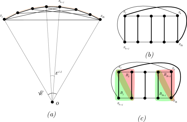
Figure 2: (a) The core gadget. (b) A different view of the core gadget. (c) A tree decomposition of the core gadget.

We observe that:

Observation 3.2.

$H_{r}$ has the following properties:

1. For any edge $e\in E(H_{r})$, we have:

   $$w(e)=\begin{cases}2r\sin(\epsilon^{3/2}/2)&\text{if $e$ is a short edge}\\ 2r\sin(k\epsilon^{3/2}/2)&\text{if $e$ is a long edge}\\ 2r\sin(\sqrt{\epsilon}/2)&\text{if $e$ is the terminal edge}\end{cases}$$ (3)

2. $w(\mathrm{MST}(H_{r}))\leq r\sqrt{\epsilon}$.

3. $w(H_{r})\geq\frac{r}{6\sqrt{\epsilon}}$ when $\epsilon\ll 1$.

Proof:  We only verify (3); other properties can be seen by direct calculation. By Taylor's expansion, each long edge of $H_{r}$ has weight $w(e)=2\sin(\frac{1}{4}(\sqrt{\epsilon}+\epsilon^{3/2}))=\frac{r}{2}(\sqrt{\epsilon}+o(\epsilon))\geq r\sqrt{\epsilon}/3$ when $\epsilon\ll 1$. Since $H_{r}$ has $k$ long edges, $w(H_{r})\geq kr\sqrt{\epsilon}/3\geq\frac{r}{6\sqrt{\epsilon}}$. $\Box$

Next, we claim that $H_{r}$ has small treewidth.

Claim 3.3.

$H_{r}$ has treewidth at most $4$.

Proof:  We construct a tree decomposition of width $4$ of $H_{r}$. In fact, we can construct a path decomposition of width $4$ for $H_{r}$. Let $B_{1},\ldots,B_{2k-2}$ be set of vertices where $B_{2i-1}=\{x_{2i-1},x_{2i+k-1},x_{2i+k}\}$ and $B_{2i}=\{x_{2i-1},x_{2i+k},x_{2i}\}$ for each $i\in[k-1]$ (see Figure 2(c)). We then add $x_{1}$ and $x_{k}$ to every $B_{i}$. Then, $\mathcal{P}=\{B_{1},\ldots,B_{2k-2}\}$ is a path decomposition of $H_{r}$ of width $4$. $\Box$

Figure 3: Paths $P_{e}$ between $x_{i}$ and $x_{i+k}$ are highlighted.

Remark: It can be seen that $H_{r}$ has $K_{4}$ as a minor, thus has treewidth at least $3$. Showing that $H_{r}$ has treewidth at least $4$ needs more work.

Lemma 3.4.

There is a constant $c$ such that any $(1+\epsilon/c)$-spanner of $H_{r}$ must have weight at least

$$\frac{w(\mathrm{MST}(H_{r}))}{6\epsilon}.$$

Proof:  Let $e$ be a long edge of $H_{r}$ and $G_{e}=H_{r}\setminus\{e\}$. We claim that the shortest path between $e$'s endpoints in $G_{e}$ must have length at least $(1+\epsilon/c)w(e)$ for some constant $c$. That implies any $(1+\epsilon/c)$-spanner of $H_{r}$ must include all long edges. The lemma then follows from Observation 3.2 since $H_{r}$ has at least $1/2\epsilon$ long edges, and each has length at least $w(\mathrm{MST}(H_{r}))/3$ for $\epsilon\ll 1$.

Suppose that $e=x_{i}x_{i+k}$. Let $P_{e}$ is a shortest path between $x_{i}$ and $x_{i+k}$ in $G_{e}$. Suppose that $w(P_{e})\leq(1+\epsilon/c)w(e)$. Since the terminal edge has length at least $3/2w(e)$, $P_{e}$ cannot contain the terminal edge. For the same reason, $P_{e}$ cannot contain two long edges. It remains to consider two cases:

1. $P_{e}$ contains exactly one long edge. Then, it must be that $P_{e}=\{x_{i},x_{i+1},x_{i+k+1},x_{i+k}\}$ (Figure 3(a)) or $P_{e}=\{x_{i},x_{i-1},x_{i+k-1},x_{i+k}\}$ (Figure 3(b)). In both case, $w(P_{i})=w(e)+4r\sin(\epsilon^{3/2}/2)\geq w(e)(1+2\frac{\sin(\epsilon^{3/2}/2)}{\sin(k\epsilon^{3/2}/2)})\geq(1+2\epsilon)w(e)$.

2. $P_{e}$ contains no long edge. Then, $P_{e}=\{x_{i},x_{i+1},\ldots,x_{i+k}\}$. Thus we have:

   $$\begin{split}\frac{w(P_{e})}{w(e)}\leavevmode\nobreak\ =\leavevmode\nobreak\ \frac{2kr\sin(\epsilon^{3/2}/2)}{2r\sin(k\epsilon^{3/2}/2)}\leavevmode\nobreak\ =\leavevmode\nobreak\ 1+\epsilon/96+o(\epsilon)\leavevmode\nobreak\ \geq\leavevmode\nobreak\ 1+\epsilon/100\end{split}$$

Thus, by choosing $c=100$, we derive a contradiction. $\Box$

Figure 4: An illustration of the recursive construction of $G_{L}$ with two levels.

Proof of Theorem 3.1. 

The construction is recursive. Let $H_{1}$ the core gadget of scale $1$. Let $s_{1}$ ($\ell_{1}$) be the length of short edges (long edges) of $H_{1}$. Let $x^{1}_{1},\ldots,x^{1}_{k}$ be break points of $H_{1}$. Let $\delta$ be the ratio of the length of a short edge to the length of the terminal edge. That is:

$$\delta=\frac{||x^{1}_{1},x^{1}_{2}||}{||x^{1}_{1},x^{1}_{2k}||}=\frac{\sin(\epsilon^{3/2}/2)}{\sin(\sqrt{\epsilon}/2)}=\epsilon+o(\epsilon)$$ (4)

Let $L=\frac{1}{\epsilon}$. We construct a set of graphs $G_{1},\ldots,G_{L}$ recursively; the output graph is $G_{L}$. We refer to $G_{i}$ is the level-$i$ graph.

Level-$1$ graph $G_{1}=H_{1}$. We refer to breakpoints of $H_{1}$ as breakpoints of $G$.

Level-$2$ graph $G_{2}$ obtained from $G_{1}$ by: (1) making $2k-1$ copies of the core gadget $H_{\delta}$ at scale $\delta$ (each $H_{\delta}$ is obtained by scaling every edge the core gadget by $\delta$), (2) for each $i\in[2k-1]$, attach each copy of $H_{\delta}$ to $G_{1}$ by identifying the terminal edge of $H_{\delta}$ and the edge between two consecutive breakpoints $x^{1}_{i}x^{1}_{i+1}$ of $G_{1}$. We then refer to breakpoints of all $H_{\delta}$ as breakpoints of $G_{2}$. (See Figure 4.) Note that by definition of $\delta$, the length of the terminal edge of $H_{\delta}$ is equal to $||x^{1}_{i},x^{1}_{i+1}||$. We say two adjacent breakpoints of $G_{2}$ consecutive if they belong to the same copy of $H_{\delta}$ in $G_{2}$ and are connected by one short edge of $H_{\delta}$.

Level-$j$ graph $G_{j}$ obtained from $G_{j-1}$ by: (1) making $(2k-1)^{j}$ copies of the core gadget $H_{\delta^{j-1}}$ at scale $\delta^{j-1}$, (2) for every two consecutive breakpoints of $G_{j-1}$, attach each copy of $H_{\delta^{j-1}}$ to $G_{j-1}$ by identifying the terminal edge of $H_{\delta^{j-1}}$ and the edge between the two consecutive breakpoints. This completes the construction.

We now show some properties of $G_{L}$. We first claim that:

Claim 3.5.

$G_{L}$ has treewidth at most $4$.

Proof:  Let $T_{1}$ be the tree decomposition of $G_{1}$ of width $5$, as guaranteed by Claim 3.3. Note that for every pair of consecutive breakpoints $x^{1}_{i},x^{1}_{i+1}$ of $G_{1}$, there is a bag, say $X_{i}$, of $T_{1}$ contains both $x^{1}_{i}$ and $x^{1}_{i+1}$. Also, there is a bag of $T_{1}$ containing both terminals of $T_{1}$.

We extend the tree decomposition $T_{1}$ to a tree decomposition $T_{2}$ of $G_{2}$ as follows. For each gadget $H_{\delta}$ attached to $G_{1}$ via consecutive breakpoints $x_{1}^{i},x^{1}_{i+1}$, we add a bag $B=\{x_{1}^{i},x^{1}_{i+1}\}$, connect $B$ to $X_{i}$ of $T_{1}$ and to the bag containing terminals of the tree decomposition of $H_{\delta}$. Observe that the resulting tree decomposition $T_{2}$ has treewidth at most $4$. The same construction can be applied recursively to construct a tree decomposition of $G_{L}$ of width at most $4$. $\Box$

Claim 3.6.

$w(\mathrm{MST}(G_{L}))=O(1)w(\mathrm{MST}(H_{1}))$.

Proof:  Let $r(\epsilon)$ be the ratio between $\mathrm{MST}(H_{1})$ and the length of the terminal edge of $H_{1}$. Note that $\mathrm{MST}(H_{1})$ is a path of short edges between $x_{1}^{1}$ and $x^{1}_{2k}$. By Observation 3.2, we have:

$$r(\epsilon)\leq\frac{r\sqrt{\epsilon}}{2r\sin(\sqrt{\epsilon}/2)}=1+\epsilon/24+o(\epsilon)\leq 1+\epsilon$$ (5)

when $\epsilon\ll 1$. When we attach copies of $H_{\delta}$ to edges between two consecutive breakpoints of $G_{1}$, by re-routing each edge of $\mathrm{MST}(H_{1})$ through the path $\mathrm{MST}(H_{\delta})$ between $H_{\delta}$'s terminals, we obtain a spanning tree of $G_{2}$ of weight at most $r(\epsilon)w(\mathrm{MST}(H_{1}))\leq(1+\epsilon)w(\mathrm{MST}(H_{1}))$. By induction, we have:

$$w(\mathrm{MST}(G_{j}))\leq(1+\epsilon)w(\mathrm{MST}(G_{j-1}))\leq(1+\epsilon)^{j-1}w(\mathrm{MST}(H_{1}))$$

This implies that $w(\mathrm{MST}(G_{L}))\leq(1+\epsilon)^{L-1}w(\mathrm{MST}(H_{1}))=O(1)w(\mathrm{MST}(H_{1}))$. $\Box$

Let $S$ be an $(1+\epsilon/100)$-spanner of $G_{L}$ ($c=100$ in Lemma 3.4). By Lemma 3.4, $S$ includes every long edge of all copies of $H_{r}$ at every scale $r$ in the construction. Recall that $||x^{1}_{1},x^{1}_{2k}||$ is the terminal edge of $G_{1}$. Let $L_{j}$ be the set of long edges of all copies of $H_{\delta^{j-1}}$ added at level $j$. Since $\frac{\mathrm{MST}(G_{1})}{||x^{1}_{1},x^{1}_{2k}||}=r(\epsilon)$, we have:

$$\begin{split}w(\mathrm{MST}(G_{1})&=\frac{r(\epsilon)}{r(\epsilon)-1}\left(w(\mathrm{MST}(G_{1}))-||x^{1}_{1},x^{1}_{2k}||\right)\geq\frac{24}{\epsilon}\left(w(\mathrm{MST}(G_{1}))-||x^{1}_{1},x^{1}_{2k}||\right)\end{split}$$ (6)

By Lemma 3.4, we have:

$$\begin{split}w(L_{1})&\geq\frac{1}{6\epsilon}w(\mathrm{MST}(G_{1}))\geq\frac{4}{\epsilon^{2}}(w(\mathrm{MST}(G_{1}))-||x^{1}_{1},x^{1}_{2k}||)\\ w(L_{2})&\geq\frac{4}{\epsilon^{2}}(w(\mathrm{MST}(G_{2}))-\mathrm{MST}(G_{1}))\\ &\ldots\\ w(L_{j})&\geq\frac{4}{\epsilon^{2}}(w(\mathrm{MST}(G_{j}))-w(\mathrm{MST}(G_{j-1})))\end{split}$$ (7)

Thus, we have:

$$w(S)\geq\sum_{j=1}^{L}w(L_{j})\geq\frac{1}{4\epsilon^{2}}(w(\mathrm{MST}(G_{L}))-||x^{1}_{1},x^{1}_{2k}||)=\Omega(\frac{1}{\epsilon^{2}})w(\mathrm{MST}(G_{L})$$

By setting $\epsilon\leftarrow\epsilon/100$, we complete the proof of Theorem 3.1. The condition on $n$ follows from the fact that $G_{L}$ has $|V(G_{L})|=O((2k-1)^{L})=O((\frac{1}{\epsilon})^{\frac{1}{\epsilon}})$ vertices. $\Box$

Part I Our Unified Framework: Applications (Section 4 and Section 5)

In this part, we show applications of our unified framework described in Theorem 1.10 in obtaining results in Section 1.

4 Applications of the Unified Framework: Fast Constructions

In this section we implement the $\mathsf{SSA}$ for each of the graph classes. By plugging the $\mathsf{SSA}$ on top of the general transformation, as provided by Theorem 1.10, we shall prove all theorems stated in Section 1. We assume that $\epsilon\ll 1$, and this is without loss of generality since we can remove this assumption by scaling $\epsilon\leftarrow\epsilon^{\prime}/c$ for any $\epsilon^{\prime}\in(0,1)$ and $c$ is sufficiently large constant. The scaling will incur a constant loss on lightness and runtime, as the dependency on $1/\epsilon$ is polynomial in all constructions below.

4.1 Euclidean Spanners and UDG Spanners

In this section we prove the following theorem.

Theorem 4.1.

Let $G=(V,E,w)$ be a $(1+\epsilon)$-spanner either for a set of $n$ points $P$ or for the unit ball graph $U$ of $P$ in $\mathbb{R}^{d}$. There is an algorithm that can compute a $(1+O(\epsilon))$-spanner $H$ of $G$ in the ACT model with lightness $O((\epsilon^{-(d+2)}+\epsilon^{-4})\log(1/\epsilon))$ in time $O(m\epsilon^{-1}(\alpha(m,n)+\epsilon^{1-d})\log(1/\epsilon))$.

We now show that Theorem 4.1 implies Theorem 1.1 and Theorem 1.3. Our construction for UDGs relies on the following result by Fürer and Kasiviswanathan [35].

Lemma 4.2 (Corollary 1 in [36]).

Given a set of $n$ points $P$ in $R^{d}$, there is an algorithm that constructs a $(1+\epsilon)$-spanner of the unit ball graph for $P$ with $O(n\epsilon^{1-d})$ edges. For $d=2$, the running time is $O(n(\epsilon^{-2}\log n))$; for $d=3$, the running time is $\tilde{O}(n^{4/3}\epsilon^{-3})$; and for $d\geq 4$, the running time is $O(n^{2-\frac{2}{(\lceil d/2\rceil+1)}+\delta}\epsilon^{-d+1}+n\epsilon^{-d})$ for any constant $\delta>0$.

Proof: [Proofs of Theorem 1.1 and Theorem 1.3]

It is known that a Euclidean $(1+\epsilon)$-spanner for a set of $n$ points $P$ in $\mathbb{R}^{d}$ with degree $O(\epsilon^{1-d})$ can be constructed in $O(n\log n)$ time in the ACT model (cf. Theorems 10.1.3 and 10.1.10 in [53]). Furthermore, when $m=O(n\epsilon^{1-d})$, we have that:

$$\alpha(m,n)\leavevmode\nobreak\ =\leavevmode\nobreak\ \alpha(nO(\epsilon^{-d}),n)\leavevmode\nobreak\ =\leavevmode\nobreak\ O(\alpha(n)+\log(\epsilon^{-d}))\leavevmode\nobreak\ =\leavevmode\nobreak\ O(\alpha(n)+d\log(1/\epsilon)).$$

Thus, Theorem 1.1 follows from Theorem 4.1.

By Lemma 4.2, we can construct sparse $(1+\epsilon)$-spanners for unit ball graphs with $m=O(n\epsilon^{1-d})$ edges in $O(n(\epsilon^{-2}\log n)$ time when $d=2$, $\tilde{O}(n^{4/3}\epsilon^{-3})$ time when $d=3$, and $O(n^{2-\frac{2}{(\lceil d/2\rceil+1)}+\delta}\epsilon^{-d+1}+n\epsilon^{-d})$ time for any constant $\delta>0$ when $d\geq 4$. Thus, Theorem 1.3 follows from Theorem 4.1. $\Box$

By Theorem 1.10, in order to prove Theorem 4.1, it suffices to implement the $\mathsf{SSA}$ for Euclidean and UDG spanners. Next, we give a detailed geometric implementation of the $\mathsf{SSA}$, hereafter $\mathsf{SSA}_{\mathsf{Geom}}$; note that the stretch parameter $t$ in the geometric setting is $1+\epsilon$. The idea is to use a Yao-graph like construction: For each node $\varphi_{C}\in\mathcal{V}$, we construct a collection of cones of angle $\epsilon$ around the representative $r(C)=\mathsf{source}(\varphi_{C})$ of the cluster $C$ corresponding to $\varphi_{C}$. Recall that we have access to a $\mathsf{source}$ function that returns the representative of each cluster in $O(1)$ time. Then for each cone, we look at all the representatives of the neighbors (in $\mathcal{G}$) of $C$ that fall into that cone, and pick to $\mathcal{E}^{\mathsf{pruned}}$ the edge that connects $r(C)$ to the representative that is closest to it.

We next analyze the running time of $\mathsf{SSA}_{\mathsf{Geom}}$, and also show that it satisfies the two properties of (Sparsity) and (Stretch) required by the abstract $\mathsf{SSA}$; these properties are described in Section 1.3. Recall that $H_{<(1+\epsilon)L}$ is the graph obtained by adding the source edges of $\mathcal{E}^{\mathsf{pruned}}$ to $H_{<L}$, which is the spanner for all edges in $G$ of weight $<L$. Note that the stretch of $H_{<L}$ is $t(1+\gamma\epsilon)$ for $t=1+\epsilon$, where $\gamma$ is a constant. Furthermore, as mentioned, we assume w.l.o.g. that $\epsilon$ is sufficiently smaller than $1$.

Figure 5: Illustration for the stretch bound proof of Lemma 4.3. Black dashed curves represent three clusters $C_{u},C_{v},C_{y}$. The solid red edge $(x,y)$ corresponds to an edge added to $\mathcal{E}^{\mathsf{pruned}}$, while the dashed red edge $(u,v)$ is not added. The green shaded region represents cone $Q_{j}$ of angle $\epsilon$ with apex at $r_{u}$.

Lemma 4.3.

$\mathsf{SSA}_{\mathsf{Geom}}$ can be implemented in $O((|\mathcal{V}|+|\mathcal{E}|)\epsilon^{1-d})$ time in the ACT model. Furthermore, 1. (Sparsity) $|\mathcal{E}^{\mathsf{pruned}}|=O(\epsilon^{1-d})|\mathcal{V}|$, and 2. (Stretch) For each edge $(\varphi_{C_{u}},\varphi_{C_{v}})\in\mathcal{E}$, $d_{H_{<(1+\epsilon)L}}(u,v)\leq t(1+s_{\mathsf{SSA}_{\mathsf{Geom}}}(\beta)\epsilon)w(u,v)$, where $(u,v)=\mathsf{source}(\varphi_{C_{u}},\varphi_{C_{v}})$, $s_{\mathsf{SSA}_{\mathsf{Geom}}}(\beta)=2(19\beta+14)$ and $\epsilon\leq\min\{\frac{1}{\gamma},\frac{1}{8\beta+6}\}$.

Proof:  We first analyze the running time. We observe that, since we can construct $\mathsf{Cone}(C_{u})$ for a single node $\varphi_{C_{u}}$ in $O(\epsilon^{1-d})$ time in the ACT model, the running time to construct all sets of cones $\{\mathsf{Cone}(C_{u})\}_{\varphi_{C_{u}}\in\mathcal{V}}$ is $O(|\mathcal{V}|\epsilon^{1-d})$. Now consider a specific node $\varphi_{C_{u}}$. For each neighbor $\varphi_{C^{\prime}}\in\mathcal{N}(\varphi_{C_{u}})$ of $\varphi_{C_{u}}$, finding the cone $Q_{j}\in\mathsf{Cone}(C_{u})$ such that $r(C^{\prime})\in Q_{j}$ takes $O(\tau)=O(\epsilon^{1-d})$ time. Thus, $\{R_{j}\}_{j=1}^{\tau}$ can be constructed in $O(|\mathcal{N}(\varphi_{C_{u}})|\epsilon^{1-d})$ time. Finding the set of representatives $\{r^{*}_{j}\}_{j=1}^{\tau}$ takes $O(|\mathcal{N}(\varphi_{C_{u}})|)$ time by calling function $\mathsf{source}(\cdot)$. Thus, the total running time to implement $\mathsf{SSA}_{\mathsf{Geom}}$ is:

$$O(|\mathcal{V}|\epsilon^{1-d})+\sum_{\varphi_{C_{u}}\in\mathcal{V}}O(|\mathcal{N}(\varphi_{C_{u}})|\epsilon^{1-d})=O((|\mathcal{V}|+|\mathcal{E}|)\epsilon^{1-d})\leavevmode\nobreak\ ,$$

as claimed.

By the construction of the algorithm, for each node $\varphi_{C}\in\mathcal{V}$, we add at most $\tau=O(\epsilon^{1-d})$ incident edges in $\mathcal{E}$ to $\mathcal{E}^{\mathsf{pruned}}$; this implies Item 1.

It remains to prove Item 2: For each edge $(\varphi_{C_{u}},\varphi_{C_{v}})\in\mathcal{E}$, the stretch in $H_{<(1+\epsilon)L}$ of the corresponding edge $(u,v)=\mathsf{source}(\varphi_{C_{u}},\varphi_{C_{v}})$ is at most $(1+s_{\mathsf{SSA}_{\mathsf{Geom}}}(\beta)\epsilon)$ with $s_{\mathsf{SSA}_{\mathsf{Geom}}}(\beta)=2(19\beta+14)$. Let $r_{u}\operatorname{\overset{\mathrm{def.}}{=}}r(C_{u})$ and $r_{v}\operatorname{\overset{\mathrm{def.}}{=}}r(C_{v})$ be the representatives of $C_{u}$ and $C_{v}$, respectively. Let $Q_{j}$ be the cone in $\mathsf{Cone}(C_{u})$ such that $r_{v}\in Q_{j}$ for some $j\in[\tau]$ (we are using the notation in $\mathsf{SSA}_{\mathsf{Geom}}$). If $r_{v}=r^{*}_{j}$, then $(u,v)\in H_{<(1+\epsilon)L}$ by the construction in $\mathsf{SSA}_{\mathsf{Geom}}$, and so the stretch is $1$. Otherwise, let $C_{y}$ be the level-$i$ cluster that contains the representative $r^{*}_{j}$. By the construction in $\mathsf{SSA}_{\mathsf{Geom}}$, there is an edge $(x,y)\in H_{<(1+\epsilon)L}$ where $x\in C_{u}$ and $y\in C_{y}$. (See Figure 5.) By property 4 of $\mathcal{G}$ in Definition 1.9, $\max\{\mathsf{Dm}(H_{<(1+\epsilon)L}[C_{u}]),\mathsf{Dm}(H_{<(1+\epsilon)L}[C_{v}]),\mathsf{Dm}(H_{<(1+\epsilon)L}[C_{y}])\}\leq\beta\epsilon L$. Note that edges in $\mathcal{E}$ have weights in $[L,(1+\epsilon)L)$ by property 3 in Definition 1.9. By the triangle inequality:

$$\begin{split}22\lVert{r_{u},r_{v}}&\leq 22\lVert{u,v}+2\beta\epsilon L\leq(1+(1+2\beta)\epsilon)L\\ 22\lVert{r_{u},r^{*}_{j}}&\leq 22\lVert{x,y}+2\beta L\leq(1+(1+2\beta)\epsilon)L\\ 22\lVert{u,v}\leq 22\lVert{r_{u},r_{v}}&+2\beta\epsilon L\qquad\mbox{ and}22\lVert{x,y}\leq 22\lVert{r_{u},r^{*}_{j}}+2\beta\epsilon L\end{split}$$ (8)

Furthermore, since $L\leq 22\lVert{u,v},22\lVert{x,y}\leq(1+\epsilon)L$, it follows that:

$$\begin{split}22\lVert{u,v}\leq(1+\epsilon)22\lVert{x,y}\quad\mbox{and}\quad 22\lVert{x,y}\leq(1+\epsilon)22\lVert{u,v}\end{split}$$ (9)

Claim 4.4.

$22\lVert{r_{v},r^{*}_{j}}\leq(8\beta+6)\epsilon L$.

Proof:  Recall that $22\lVert{r_{u},r^{*}_{j}}\leq 22\lVert{r_{u},r_{v}}$. Let $p$ be the projection of $r_{j}^{*}$ onto the segment $r_{u}r_{v}$ (see Figure 5). Since $\angle r_{v}r_{u}r^{*}_{j}\leq\epsilon$, $22\lVert{r_{j}^{*},p}\leq\sin(\epsilon)22\lVert{r_{u},r^{*}_{j}}\leq\sin(\epsilon)22\lVert{r_{u},r_{v}}\leavevmode\nobreak\ \leq\leavevmode\nobreak\ \epsilon(1+(1+2\beta)\epsilon)L$. We have:

$$\begin{split}22\lVert{r_{v},r^{*}_{j}}&\leq 22\lVert{p,r^{*}_{j}}+22\lVert{r_{v},p}\leq 22\lVert{p,r^{*}_{j}}+22\lVert{r_{u},r_{v}}-(22\lVert{r_{u},r_{j}^{*}}-22\lVert{r_{j}^{*},p})\\ &\leq(22\lVert{r_{u},r_{v}}-22\lVert{r_{u},r_{j}^{*}})+2\epsilon(1+(1+2\beta)\epsilon)L\end{split}$$ (10)

We now bound $(22\lVert{r_{u},r_{v}}-22\lVert{r_{u},r_{j}^{*}})$. By Equation 8 and Equation 9, it holds that:

$$\begin{split}22\lVert{r_{u},r_{v}}-22\lVert{r_{u},r_{j}^{*}}&\leq 22\lVert{u,v}+2\beta\epsilon L-(22\lVert{x,y}-2\beta\epsilon L)\leq(4\beta+1+\epsilon)\epsilon L\end{split}$$ (11)

Plugging Equation 11 into Equation 10, we get:

$$\begin{split}22\lVert{r_{v},r_{j}^{*}}&\leq(4\beta+1+\epsilon)\epsilon L+2\epsilon(1+(1+2\beta)\epsilon)L\leq(8\beta+6)\epsilon L\leavevmode\nobreak\ \qquad\mbox{(since }\epsilon\leq 1),\end{split}$$

as claimed. This completes the proof of 4.4. $\Box$

Next we continue with the proof of Lemma 4.3. By 4.4, $22\lVert{r_{v},r^{*}_{j}}<L$ when $\epsilon<1/(8\beta+6)$. If the input graph is a UDG, then $\mathcal{E}\not=\emptyset$ only if $L\leq 1$. Thus, $22\lVert{r_{v},r^{*}_{j}}\leq 1$ and hence, there is an edge $(r_{v},r^{*}_{j})$ of length $22\lVert{r_{v},r^{*}_{j}}$ in the input UDG. (This is the only place, other than starting our construction with a $(1+\epsilon)$-spanner for the input UDG, where we exploit the fact that the input graph is a UDG.)

Since $22\lVert{r_{v},r^{*}_{j}}<L$, the distance between $r_{v}$ and $r^{*}_{j}$ is preserved up to a factor of $(1+\gamma\epsilon)$ in $H_{<L}$. That is, $d_{H_{<(1+\epsilon)L}}(r_{v},r^{*}_{j})\leq(1+\gamma\epsilon)22\lVert{r_{v},r^{*}_{j}}$.

Note that $r_{u},r_{v},r_{j}^{*}$ are all in the input point set $P$ by the definition of representatives. By the triangle inequality, it follows that:

$$\begin{split}d_{H_{<(1+\epsilon)L}}(u,v)&\leq d_{H_{<(1+\epsilon)L}}(u,x)+22\lVert{x,y}+d_{H_{<(1+\epsilon)L}}(y,r_{j}^{*})+d_{H_{<(1+\epsilon)L}}(r_{j}^{*},r_{v})+d_{H_{<(1+\epsilon)L}}(r_{v},v)\\ &\leq\beta\epsilon L+22\lVert{x,y}+\beta\epsilon L+(1+\gamma\epsilon)22\lVert{r_{v},r^{*}_{j}}+\beta\epsilon L\\ &\leq 22\lVert{x,y}+3\beta\epsilon L+\underbrace{(1+\gamma\epsilon)}_{\leq\leavevmode\nobreak\ 2\text{ since }\epsilon\leavevmode\nobreak\ \leq\leavevmode\nobreak\ 1/\gamma}(8\beta+6)\epsilon L\qquad\mbox{(by \lx@cref{creftypecap~refnum}{clm:ACT-rvrj})}\\ &\leq 22\lVert{x,y}+(19\beta+12)\epsilon L\end{split}$$ (12)

By Equation 9, $22\lVert{x,y}\leavevmode\nobreak\ \leq\leavevmode\nobreak\ (1+\epsilon)22\lVert{u,v}\leq 22\lVert{u,v}+(1+\epsilon)\epsilon L\leq 22\lVert{u,v}+2\epsilon L$. Thus, by Equation (12):

$$d_{H_{<(1+\epsilon)L}}(u,v)\leq 22\lVert{u,v}+(19\beta+14)\epsilon L\stackrel{{\scriptstyle 22\lVert{u,v}\geq L/2}}{{\leq}}(1+2(19\beta+14)\epsilon)22\lVert{u,v}.$$

That is, the stretch of $(u,v)$ in $H_{<(1+\epsilon)L}$ is at most $1+s_{\mathsf{SSA}_{\mathsf{Geom}}}(\beta)\epsilon$ with $s_{\mathsf{SSA}_{\mathsf{Geom}}}(\beta)=2(19\beta+14)$. $\Box$

Remark 4.5.

$\mathsf{SSA}_{\mathsf{Geom}}$ can be implemented slightly faster, within time $O(|\mathcal{V}|\epsilon^{1-d}+|\mathcal{E}|\log(1/\epsilon))$, by using a data structure that allows us to search for the cone that a representative belongs to in $O(\log(1/\epsilon))$ time. Such a data structure is described in Theorem 5.3.2 in the book by Narasimhan and Smid [53].

Proof: [Proof of Theorem 4.1] We use $\mathsf{SSA}_{\mathsf{Geom}}$ in place of the abstract $\mathsf{SSA}$ in Theorem 1.10 to construct the light spanner. By Lemma 4.3, we have $s_{\mathsf{SSA}}(\beta)=2(19\beta+14)$, $\chi=O(\epsilon^{1-d})$ and $\tau(m^{\prime},n^{\prime})=O(\epsilon^{1-d})$. Thus, by plugging in the values of $\chi$ and $\tau$, we obtain the lightness and the running time as required by Theorem 4.1. The stretch of the spanner is $(1+\epsilon)(1+(s_{\mathsf{SSA}}(O(1))+O(1))\epsilon)=(1+O(\epsilon))$ when $\epsilon\leq 1$. $\Box$

4.2 General Graphs

In this section, we prove Theorem 1.2 by giving a detailed implementation of $\mathsf{SSA}$ for general graphs, hereafter $\mathsf{SSA}_{\mathsf{Gen}}$. Here we have $t=2k-1$ for an integer parameter $k\geq 2$. We will use as a black-box the linear-time construction of sparse spanners in general unweighted graphs by Halperin and Zwick [41].

Theorem 4.6 (Halperin-Zwick [41]).

Given an unweighted $n$-vertex graph $G$ with $m$ edges, a $(2k-1)$-spanner of $G$ with $O(n^{1+\frac{1}{k}})$ edges can be constructed deterministically in $O(m+n)$ time, for any $k\geq 2$.

We next analyze the running time of $\mathsf{SSA}_{\mathsf{Gen}}$, and also show that it satisfies the two properties of (Sparsity) and (Stretch) required by the abstract $\mathsf{SSA}$; these properties are described in Section 1.3.

Lemma 4.7.

$\mathsf{SSA}_{\mathsf{Gen}}$ can be implemented in $O(|\mathcal{V}|+|\mathcal{E}|)$ time. Furthermore, 1. (Sparsity) $\mathcal{E}^{\mathsf{pruned}}=O(n^{1/k})|\mathcal{V}|$, and 2. (Stretch) For each edge $(\varphi_{C_{u}},\varphi_{C_{v}})\in\mathcal{E}$, $d_{H_{<(1+\epsilon)L}}(u,v)\leq(2k-1)(1+s_{\mathsf{SSA}_{\mathsf{Gen}}}(\beta)\epsilon)w(u,v)$, where $(u,v)=\mathsf{source}(\varphi_{C_{u}},\varphi_{C_{v}})$, $s_{\mathsf{SSA}_{\mathsf{Gen}}}(\beta)=(2\beta+1)$ and $\epsilon\leq 1$.

Proof:  The running time of $\mathsf{SSA}_{\mathsf{Gen}}$ follows directly from Theorem 4.6. Also, by Theorem 4.6, $|\mathcal{E}^{\mathsf{pruned}}|=O(|\mathcal{V}|^{1+1/k})=O(n^{1/k}|\mathcal{V}|)$; this implies Item 1.

It remains to prove Item 2: For each edge $(\varphi_{C_{u}},\varphi_{C_{v}})\in\mathcal{E}$, the stretch in $H_{<(1+\epsilon)L}$ (constructed as described in $\mathsf{SSA}$) of the corresponding edge $(u,v)=\mathsf{source}(\varphi_{C_{u}},\varphi_{C_{v}})$ is at most $(2k-1)(1+(2\beta+1)\epsilon)w(u,v)$. Recall that $H_{<(1+\epsilon)L}$ is the graph obtained by adding the source edges of $\mathcal{E}^{\mathsf{pruned}}$ to $H_{<L}$.

Let $(u_{1},v_{1})$ be the edge in $E_{J}$ that corresponds to the edge $(\varphi_{C_{u}},\varphi_{C_{v}})$. By Theorem 4.6, there is a path $P$ between $u_{1}$ and $v_{1}$ in $J$ such that $P$ contains at most $2k-1$ edges. We write $P=(u_{1}=x_{0},(x_{0},x_{1}),x_{1},(x_{1},x_{2}),\ldots,x_{p}=v_{1})$ as an alternating sequence of vertices and edges. Let $\mathcal{P}=(\varphi_{0},(\varphi_{0},\varphi_{1}),\varphi_{1},(\varphi_{1},\varphi_{2}),\ldots,\varphi_{p})$ be a path of $\mathcal{G}$, written as an alternating sequence of vertices and edges, that is obtained from $P$ where $\varphi_{j}$ corresponds to $x_{j}$, $1\leq j\leq p$. Note that $\varphi_{1}=\varphi_{C_{u}}$ and $\varphi_{p}=\varphi_{C_{v}}$.

Figure 6: A path from $u$ to $v$.

Let $\{y_{i}\}_{i=0}^{p}$ and $\{z_{i}\}_{i=0}^{p}$ be two sequences of vertices of $G$ such that (a) $z_{0}=u$ and $y_{p}=v$, and (b) $(y_{i-1},z_{i})$ is the edge in $G$ corresponding to edge $(\varphi_{i-1},\varphi_{i})$ in $\mathcal{P}$, for $1\leq i\leq p$. Let $Q_{i}$, $0\leq i\leq p$, be a shortest path in $H_{<L}[C_{i}]$ between $z_{i}$ and $y_{i}$, where $C_{i}$ is the cluster corresponding to $\varphi_{i}$. See Figure 6 for an illustration. Observe that $w(Q_{i})\leq\beta\epsilon L$ by property 4 in Definition 1.9. Let $P^{\prime}=Q_{0}\circ(y_{0},z_{1})\circ\ldots\circ Q_{p}$ be a (possibly non-simple) path from $u$ to $v$ in $H_{<(1+\epsilon)L}$; here $\circ$ is the path concatenation operator.

$$\begin{split}w(P^{\prime})&\leq(2k-1)(1+\epsilon)L+(2k)\beta\epsilon L\leq(2k-1)(1+\epsilon+2\beta\epsilon)L\\ &\leq(2k-1)(1+(2\beta+1)\epsilon)w(u,v)\qquad\mbox{(since $w(u,v)\geq L$)}\\ \end{split}$$ (13)

Thus, the stretch of edge $(u,v)$ is at most $(2k-1)(1+(2\beta+1)\epsilon)$, as required. $\Box$

Proof: [Proof of Theorem 1.2] We use algorithm $\mathsf{SSA}_{\mathsf{Gen}}$ in place of the abstract $\mathsf{SSA}$ in Theorem 1.10 to construct the light spanner. By Lemma 4.3, we have $s_{\mathsf{SSA}}(\beta)=(2\beta+14)$, $\chi=O(n^{1/k})$ and $\tau(m^{\prime},n^{\prime})=O(1)$. Thus, by plugging in the values of $\chi$ and $\tau$, we obtain the lightness and the running time as required by Theorem 1.2. The stretch of the spanner is $(2k-1)(1+(s_{\mathsf{SSA}}(O(1))+O(1))\epsilon)=(2k-1)(1+O(\epsilon))$. By scaling, we get the required stretch of $(2k-1)(1+\epsilon)$. $\Box$

4.3 Minor-free Graphs

In this section, we prove a weaker version of Theorem 1.4, where the running time is $O(nr\sqrt{r}\alpha(nr\sqrt{r},n))$. In Section 9 we show how to achieve a linear running time, via an adaptation of our framework (described in detail in Section 6) to minor-free graphs.

The implementation of the abstract algorithm $\mathsf{SSA}$ for minor-free graphs, hereafter $\mathsf{SSA}_{\mathsf{Minor}}$, simply outputs the edge set $\mathcal{E}$. Note that the stretch in this case is $t=1+\epsilon$.

We next analyze the running time of $\mathsf{SSA}_{\mathsf{Minor}}$, and also show that it satisfies the two properties of (Sparsity) and (Stretch) required by the abstract $\mathsf{SSA}$.

Lemma 4.8.

$\mathsf{SSA}_{\mathsf{Minor}}$ can be implemented in $O((|\mathcal{V}|+|\mathcal{E}|))$ time. Furthermore, 1. (Sparsity) $\mathcal{E}^{\mathsf{pruned}}=O(r\sqrt{\log r})|\mathcal{V}|$, and 2. (Stretch) For each edge $(\varphi_{C_{u}},\varphi_{C_{v}})\in\mathcal{E}$, $d_{H_{<(1+\epsilon)L}}(u,v)\leq(1+\epsilon)(1+s_{\mathsf{SSA}_{\mathsf{Minor}}}(\beta)\epsilon)w(u,v)$, where $(u,v)=\mathsf{source}(\varphi_{C_{u}},\varphi_{C_{v}})$, $s_{\mathsf{SSA}_{\mathsf{Minor}}}(\beta)=0$ and $\epsilon\leq 1$.

Proof:  The running time of $\mathsf{SSA}_{\mathsf{Minor}}$ follows trivially from the construction. Noting that $\mathcal{G}$ is a minor of the input graph $G$, $\mathcal{G}$ is $K_{r}$-minor-free. Thus, $|\mathcal{E}|=O(r\sqrt{\log r})|\mathcal{V}|$ by the sparsity of minor-free graphs [45, 59]; this implies Item 1. Since we take every edge of $\mathcal{E}$ to $\mathcal{E}^{\mathsf{pruned}}$, the stretch is $1$ and hence $s_{\mathsf{SSA}_{\mathsf{Minor}}}(\beta)=0$, yielding Item 2. $\Box$

We are now ready to prove a weaker version of Theorem 1.4 for minor-free graphs, where the running time is $O(nr\sqrt{r}\alpha(nr\sqrt{r},n))$.

Proof: [Proof of Theorem 1.4] We use algorithm $\mathsf{SSA}_{\mathsf{Minor}}$ in place of the abstract $\mathsf{SSA}$ in Theorem 1.10 to construct the light spanner. By Lemma 4.3, we have $s_{\mathsf{SSA}}(\beta)=0$, $\chi=O(r\sqrt{\log r})$ and $\tau(m^{\prime},n^{\prime})=O(1)$. Thus, by plugging in the values of $\chi$ and $\tau$, we obtain the lightness claimed in Theorem 1.4 and a running time of $O(nr\sqrt{r}\alpha(nr\sqrt{r},n))$, for a constant $\epsilon$. The stretch of the spanner is:

$$(1+\epsilon)(1+(s_{\mathsf{SSA}}(O(1))+O(1))\epsilon)=(1+O(\epsilon))$$

By scaling, we get a stretch of $(1+\epsilon)$. $\Box$

5 Applications of the Unified Framework: Fine-Grained Optimality

In this section, we use the framework outlined in Section 1.3 to obtain all results regarding fine-grained lightness bounds stated in Section 1.2: Theorem 1.5, Theorem 1.6, Theorem 1.7, and Theorem 1.8. We do so by introduce another layer of abstraction via an object that we call general sparse spanner oracle ($\mathsf{GSSO}$) in Section 5.1: we show that the existence of $\mathsf{GSSO}$ implies the existence of light spanners. In Section 5.2, we construct $\mathsf{GSSO}$es for different class of graphs: general graphs, high dimensional Euclidean spanners, and Steiner Euclidean spanners. Finally, in Section 5.3, we construct a light spanner for minor-free graphs by directly implementing $\mathsf{SSO}$. See Figure 1 for relationships between theorems/lemmas.

5.1 General Sparse Spanner Oracles

We introduce the notion of a general sparse spanner oracle ($\mathsf{GSSO}$). Our $\mathsf{GSSO}$ for stretch $t=1+\epsilon$ coincides with a notion called spanner oracle, introduced by Le [47]; nonetheless, our goal is much more ambitious: First we wish to optimize the fine-grained dependencies and second we wish to do so while considering a much wider regime of the stretch parameter $t$, which may even depend on $n$.

Definition 5.1 (General Sparse Spanner Oracle).

Let $G$ be an edge-weighted graph and let $t>1$ be a stretch parameter. A general sparse spanner oracle ($\mathsf{GSSO}$) of $G$ for a given stretch $t$ is an algorithm that, given a subset of vertices $T\subseteq V(G)$ and a distance parameter $L>0$, outputs in polynomial time a subgraph $S$ of $G$ such that for every pair of vertices $x,y\in T,x\not=y$ with $L\leq d_{G}(x,y)<2L$:

$$d_{S}(x,y)\leq t\cdot d_{G}(x,y).$$ (14)

We denote a $\mathsf{GSSO}$ of $G$ with stretch $t$ by $\mathcal{O}_{G,t}$, and its output subgraph is denoted by $\mathcal{O}_{G,t}(T,L)$, given two parameters $T\subseteq V(G)$ and $L>0$.

Definition 5.2 (Sparsity).

Given a $\mathsf{GSSO}$ $\mathcal{O}_{G,t}$ of a graph $G$, we define weak sparsity and strong sparsity of $\mathcal{O}_{G,t}$, denoted by $\mathtt{Ws}_{\mathcal{O}_{G,t}}$ and $\mathtt{Ss}_{\mathcal{O}_{G,t}}$ respectively, as follows:

$$\begin{split}\mathtt{Ws}_{\mathcal{O}_{G,t}}&=\sup_{T\subseteq V,L\in^{+}}\frac{w\left(\mathcal{O}_{G,t}(T,L)\right)}{|T|L}\\ \mathtt{Ss}_{\mathcal{O}_{G,t}}&=\sup_{T\subseteq V,L\in^{+}}\frac{|E\left(\mathcal{O}_{G,t}(T,L)\right)|}{|T|}\end{split}$$ (15)

We observe that:

$$\mathtt{Ws}_{\mathcal{O}_{G,t}}\leq t\cdot\mathtt{Ss}_{\mathcal{O}_{G,t}},$$ (16)

since every edge $E\left(\mathcal{O}_{G,t}(T,L)\right)$ must have weight at most $t\cdot L$; indeed, otherwise we can remove it from $\mathcal{O}_{G,t}(T,L)$ without affecting the stretch. Thus, when $t$ is constant, strong sparsity implies weak sparsity; note, however, that this is not necessarily the case when $t$ is super-constant.

Our main result in this section is to show that for stretch $t\geq 2$, we can construct a light spanner with lightness bound roughly $O(\frac{1}{\epsilon})$ times the sparsity of the spanner oracle (Theorem 5.3). For stretch $t=1+\epsilon$, we can construct a light spanner with lightness bound roughly $O(\frac{1}{\epsilon})$ times the sparsity of the spanner oracle plus an additive factor $1/\epsilon^{2}$.

Theorem 5.3.

Let $G$ be an arbitrary edge-weighted graph that admits a $\mathsf{GSSO}$ $\mathcal{O}_{G,t}$ of weak sparsity $\mathtt{Ws}_{\mathcal{O}_{G,t}}$ for $t\geq 2$. Then for any $\epsilon>0$, we can construct in polynomial time a $t(1+\epsilon)$-spanner for $G$ with lightness $\tilde{O}_{\epsilon}\left(\frac{\mathtt{Ws}_{\mathcal{O}_{G,t}}}{\epsilon}\right)$

Theorem 5.4.

Let $G$ be an arbitrary edge-weighted graph that admits a $\mathsf{GSSO}$ $\mathcal{O}_{G,1+\epsilon}$ of weak sparsity $\mathtt{Ws}_{\mathcal{O}_{G,1+\epsilon}}$ for any $\epsilon>0$. Then there exists an $(1+O(\epsilon))$-spanner for $G$ with lightness $\tilde{O}_{\epsilon}\left(\frac{\mathtt{Ws}_{\mathcal{O}_{G,t}}}{\epsilon}+\frac{1}{\epsilon^{2}}\right)$.

In both Theorem 5.3 and Theorem 5.4, $\tilde{O}_{\epsilon}(.)$ hides a factor of $\log\frac{1}{\epsilon}$. The proofs of these theorem are presented in Section 5.1.

The bound in Theorem 5.4 improves over the lightness bound due to Le [49] by a factor of $\frac{1}{\epsilon^{2}}$. The stretch of $S$ in Theorem 5.4 is $1+O(\epsilon)$, but we can scale it down to $(1+\epsilon)$ while increasing the lightness by a constant factor. Moreover, this bound is optimal, as we shall assert next. First, the additive factor $\frac{\mathtt{Ws}_{\mathcal{O}_{G,t}}}{\epsilon}$ is unavoidable: the authors showed in [50] that there exists a set of $n$ points in $\mathbb{R}^{d}$ such that any $(1+\epsilon)$-spanner for it must have lightness $\Omega(\epsilon^{-d})$, while the result of Le [49] implies that point sets in $\mathbb{R}^{d}$ have $\mathsf{GSSO}$es with weak sparsity $O(\epsilon^{1-d})$. Second, the additive factor $\frac{1}{\epsilon^{2}}$ is tight by the following theorem.

Theorem 5.5.

For any $\epsilon<1$ and $n\geq(\frac{1}{\epsilon})^{\Theta(\frac{1}{\epsilon})}$, there is an $n$-vertex graph $G$ admitting a $\mathsf{GSSO}$ of stretch $(1+\epsilon)$ with weak sparsity $O(1)$ such that any $(1+\epsilon)$-spanner of $G$ must have lightness $\Omega(\frac{1}{\epsilon^{2}})$.

Proof:  Le (Theorem 1.3 in [49]), building upon the work of Krauthgamer, Nguy$\tilde{\hat{\mbox{e}}}$n and Zondiner [46], showed that graphs with treewidth $\mathsf{tw}$ have a $1$-spanner oracle with weak sparsity $O(\mathsf{tw}^{4})$. Since the treewidth of $G$ in Theorem 3.1 is $4$, it has a $1$-spanner oracle with weak sparsity $O(1)$; this implies Theorem 5.5. $\Box$

Light spanners from GSSO. 

We now turn to proving Theorem 5.3 and Theorem 5.4. We do so by providing an implementation of $\mathsf{SSO}$ using a $\mathsf{GSSO}$. We assume that we are given a $\mathsf{GSSO}$ $\mathcal{O}_{G,t}$ with weak sparsity $\mathtt{Ws}_{\mathcal{O}_{G,t}}$. We denote the algorithm by $\mathsf{SSO}_{\mathsf{Oracle}}$. We assume that every edge in $G$ is a shortest path between its endpoints; otherwise, we can safely remove them from the graph.

We now show that $\mathsf{SSO}_{\mathsf{Oracle}}$ has all the properties as described in the abstract $\mathsf{SSO}$.

Lemma 5.6.

Let $F$ be the output of $\mathsf{SSO}_{\mathsf{Oracle}}$. Then $w(F)=O(\mathtt{Ws}_{\mathcal{O}_{G,t}})L\cdot|\mathcal{V}|$. Furthermore, $d_{H_{<2L}}(u,v)\leq t(1+s_{\mathsf{SSO}_{\mathsf{Oracle}}}(\beta)\epsilon)w(u,v)$ for every edge $(u,v)$ corresponding to an edge in $\mathcal{E}$, where $s_{\mathsf{SSO}_{\mathsf{Oracle}}}(\beta)=4\beta$ and $\epsilon$ is sufficiently smaller than $1$, in particular $\epsilon\leq 1/(4\beta)$.

Proof:  Since we only choose exactly one vertex in $S$ per node in $\mathcal{G}$, $|S|=|\mathcal{V}|$. By the definition of the sparsity of an oracle (Definition 5.2), $w(F)\leq\mathtt{Ws}_{\mathcal{O}_{G,t}}(L/2)\cdot|S|+\mathtt{Ws}_{\mathcal{O}_{G,t}}L\cdot|S|+\mathtt{Ws}_{\mathcal{O}_{G,t}}2L\cdot|S|=O(\mathtt{Ws}_{\mathcal{O}_{G,t}})L\cdot|\mathcal{V}|$; this implies the first claim.

Let $(u,v)$ be an edge in $G$ corresponding to an edge $(\varphi_{C_{u}},\varphi_{C_{v}})\in\mathcal{E}$. We have that $L\leq w(u,v)<2L$ by property 3 in Definition 1.9. By the construction of $S$ in $\mathsf{SSO}_{\mathsf{Oracle}}$, there are two vertices $u_{1}\in C_{u}$ and $v_{1}\in C_{v}$ that are in $S$. Let $P_{u_{1},u}$ ($P_{v_{1},v}$) be the shortest path in $H_{<L}[C_{u}]$ ($H_{<L}[C_{v}]$) between $u$ and $u_{1}$ ($v$ and $v_{1}$). By property 4 in Definition 1.9, we have that $\max\{w(P_{u_{1},u}),w(P_{v_{1},v})\}\leq\beta\epsilon L$. By the triangle inequality, we have:

$$d_{G}(u_{1},v_{1})\leq w(u,v)+2\beta\epsilon L<(2+2\beta\epsilon)L\leq 4L,$$ (18)

since $\epsilon\leq 1/\beta$. Also by the triangle equality, it follows that:

$$d_{G}(u_{1},v_{1})\geq w(u,v)-2\beta\epsilon L\geq(1-2\beta\epsilon L)\geq L/2,$$ (19)

since $\epsilon\leq\frac{1}{4\beta}$. Thus, $d_{G}(u_{1},v_{1})\in[L/2,2L)$. It follows by the definition of $\mathsf{GSSO}$ (Definition 5.1) that there is a path, say $P_{u_{1},v_{1}}$, of weight at most $t\cdot d_{G}(u_{1},v_{1})$ between $u_{1}$ and $v_{1}$ in the graph induced by $F$. Let $P_{u,v}=P_{u_{1},u}\circ P_{u_{1},v_{1}}\circ P_{v,v_{1}}$ be the path between $u$ and $v$ obtained by concatenating $P_{u_{1},u},P_{u_{1},v_{1}},P_{v,v_{1}}$. By the triangle inequality, it follows that:

$$\begin{split}w(P_{u,v})&\leq w(P_{u_{1},v_{1}})+w(P_{u_{1},u})+w(P_{v_{1},v})\leq t\cdot d_{G}(u_{1},v_{1})+2\epsilon\beta L\\ &\stackrel{{\scriptstyle\mbox{\footnotesize{\lx@cref{creftype~refnum}{eq:oracleStretch-uv-up}}}}}{{=}}t\cdot(w(u,v)+2\epsilon\beta L)+2\epsilon\beta L\\ &\leq t\cdot(w(u,v)+4\epsilon\beta L)\leq t\cdot(1+4\epsilon\beta)w(u,v)\qquad\mbox{(since $w(u,v)\geq L$ and $t\geq 1$)},\end{split}$$ (20)

as desired. $\Box$

Proof: [Proof of Theorem 5.3] By Theorem 1.10 and Lemma 5.6, we can construct in polynomial time a spanner $H$ with stretch $t(1+(2s_{\mathsf{SSO}_{\mathsf{Oracle}}}(O(1))+O(1))\epsilon)$ where $s_{\mathsf{SSO}_{\mathsf{Oracle}}}(\beta)=8\beta$. Thus, the stretch of $H$ is $t(1+O(\epsilon))$; we then can recover stretch $t(1+\epsilon)$ by scaling. The lightness of $H$ is $\tilde{O}_{\epsilon}((\chi\epsilon^{-1}))$ with $\chi=O(\mathtt{Ws}_{\mathcal{O}_{G,t}})$. That implies a lightness of $\tilde{O}_{\epsilon}((\mathtt{Ws}_{\mathcal{O}_{G,t}}\epsilon^{-1}))$ as claimed. $\Box$

Proof: [Proof of Theorem 5.4] The proof follows the same line of the proof of Theorem 5.3. The difference is that we apply Lemma 5.6 and Theorem 1.10 with $t=1+\epsilon$ to construct $H$. Thus, the stretch of $H$ is $t(1+O(\epsilon))=1+O(\epsilon)$. Since $\chi=\mathtt{Ws}_{\mathcal{O}_{G,1+\epsilon}}$, the lightness is $\tilde{O}_{\epsilon}\left(\frac{\mathtt{Ws}_{\mathcal{O}_{G,t}}}{\epsilon}+\frac{1}{\epsilon^{2}}\right)$ as claimed. $\Box$

5.2 Constructing General Sparse Spanner Oracles

We construct $\mathsf{GSSO}$es for different class of graphs: general graphs, high dimensional metric spanners, and Steiner Euclidean spanners. This together with Theorem 5.3 and Theorem 5.4 give Theorem 1.6, Theorem 1.7, and Theorem 1.8.

5.2.1 General graphs and high dimensional metric spaces: Proof of Theorem 1.6 and Theorem 1.8

Theorem 5.7.

The following $\mathsf{GSSO}$es exist.

1. For any weighted graph $G$ and any $k\geq 2$, $\mathtt{Ws}_{\mathcal{O}_{G,2k-1}}=O(g(n,k))$.

2. For the complete weighted graph $G$ corresponding to any Euclidean space (in any dimension) and for any $t\geq 1$, $\mathtt{Ws}_{\mathcal{O}_{G,O(t)}}=O(tn^{\frac{1}{t^{2}}}\log n)$.

3. For the complete weighted graph $G$ corresponding to any finite $\ell_{p}$ normed space for $p\in(1,2]$ and for any $t\geq 1$, $\mathtt{Ws}_{\mathcal{O}_{G,O(t)}}=O(tn^{\frac{\log t}{t^{p}}}\log n)$.

Theorem 1.6 follows directly from Theorem 5.3 and Item (1) of Theorem 5.7; Theorem 1.8 follows directly from Theorem 5.3 and Item (2) and Item (3) of Theorem 5.7 with $\epsilon=1/2$; any constant $\epsilon<1$ works. See Figure 1 for a graphical illustration of the relationships between these theorems. We now focus on proving Theorem 5.7.

General graphs. 

For a given graph $G(V,E)$ and $T\subseteq V$, we construct another weighted graph $G_{T}(T,E_{T},w_{T})$ with vertex set $T$ such that for every two vertices $u,v$ that form a critical pair, we add an edge $(u,v)$ with weight $w_{T}(u,v)=d_{G}(u,v)$.

We apply the greedy algorithm [2] to $G_{T}$ with $t=2k-1$ and return the output of the greedy spanner, say $S_{T}$, (after replacing each artificial edge by the shortest path between its endpoints) as the output of the oracle $\mathcal{O}_{G,2k-1}$. We now bound the weak sparsity of $\mathcal{O}_{G,2k-1}$.

It was shown (Lemma 2 in [2]) that $S_{T}$ has girth $2k+1$ and hence has at most $g(|T|,k)|T|\leq g(n,k)|T|$ edges. It follows that $w(S_{T})\leavevmode\nobreak\ \leq\leavevmode\nobreak\ |g(n,k)|T|2L\leavevmode\nobreak\ =\leavevmode\nobreak\ O(g(n,k))|T|L$. That implies:

$$\mathtt{Ws}_{\mathcal{O}_{G,2k-1}}=\sup_{T\subseteq V,L\in\mathcal{R}^{+}}\frac{O(g(n,k))|T|L}{|T|L}=O(n^{1/k}).$$

This implies Item (1) of Theorem 5.7.

High dimensional metric spaces. 

Let $(X,d_{X})$ be a metric space and $\mathcal{P}$ be a partition of $(X,d_{X})$ into clusters. We say that $\mathcal{P}$ is $\Delta$-bounded if $\mathsf{Dm}(P)\leq\Delta$ for every $P\in\mathcal{P}$. For each $x\in X$, we denote the cluster containing $x$ in $\mathcal{P}$ by $\mathcal{P}(x)$. The following notion of $(t,\Delta,\delta$)-decomposition was introduced by Filtser and Neiman [33].

Definition 5.8 (($t,\Delta,\eta$)-decomposition).

Given parameters $t\geq 1,\Delta>0,\eta\in[0,1]$, a distribution $\mathcal{D}$ over partitions of $(X,d_{X})$ is a $(t,\Delta,\eta)$-decomposition if:

• Every partition $\mathcal{P}$ drawn from $\mathcal{D}$ is $t\cdot\Delta$-bounded.

• For every $x\not=y\in X$ such that $d_{X}(x,y)\leq\Delta$, $\operatorname{\mathtt{Pr}}\limits_{\mathcal{P}\sim\mathcal{D}}[\mathcal{P}(x)=\mathcal{P}(y)]\geq\eta$

$(X,d)$ is $(t,\eta)$-decomposable if it has a ($t,\Delta,\eta$)-decomposition for any $\Delta>0$.

Claim 5.9.

If $(X,d_{X})$ is $(t,\eta)$-decomposable, it has a $\mathsf{GSSO}$ $\mathcal{O}_{X,O(t)}$ with sparsity $\mathtt{Ws}_{\mathcal{O}_{X,O(t)}}=O(\frac{t\log|X|}{\eta})$. Furthermore, there is a polynomial time Monte Carlo algorithm constructing $\mathcal{O}_{X,O(t)}$ with constant success probability.

Proof:  Let $T$ be a set of terminals given to the oracle $\mathcal{O}_{X,O(t)}$. Let $\mathcal{D}$ be a $(t,2L,\eta)$-decomposition of $(X,d_{X})$.

Initially the spanner $S$ has $V(S)=T$ and $E(S)=\emptyset$. We sample $\rho=\frac{2\ln|T|}{\eta}$ partitions from $\mathcal{D}$, denoted by $\mathcal{P}_{1},\ldots,\mathcal{P}_{\rho}$. For each $i\in[\rho]$ and each cluster $C\in\mathcal{P}_{i}$, if $|T\cap C|\geq 2$, we pick a terminal $t\in C$ and add to $S$ edges from $t$ to all other terminals in $C$. We then return $S$ as the output of the oracle.

For each partition $\mathcal{P}_{i}$, the set of edges added to $S$ forms a forest. That implies we add to $S$ at most $|T|-1$ edges per partition. Thus, $|E(S)|\leq(|T|-1)\rho=O(\frac{|T|\log|T|}{\eta})$. Observe that $w(S)\leq|E(S)|\cdot t2L=(\frac{2|T|tL\log|T|}{\eta})$ since each edge has weight at most $t\cdot(2L)$. Thus, $\mathtt{Ws}_{\mathcal{O}}=O(\frac{t\log|T|}{\eta})=O(\frac{t\log|X|}{\eta})$.

It remains to show that with constant probability, $d_{S}(x,y)\leq O(t)d_{X}(x,y)$ for every $x\not=y\in T$ such that $L\leq d_{X}(x,y)<2L$. Observe by construction that if $x$ and $y$ fall into the same cluster in any partition, there is a $2$-hop path of length at most $4tL=O(t)d_{X}(x,y)$. Thus, we only need to bound the probability that $x$ and $y$ are clustered together in some partition. Observe that the probability that there is no cluster containing both $x$ and $y$ in $\rho$ partitions is at most:

$$(1-\eta)^{\rho}=(1-\eta)^{\frac{2\ln|T|}{\eta}}\leq\frac{1}{|T|^{2}}$$

Since there are at most $\frac{|T|^{2}}{2}$ distinct pairs, by union bound, the desired probability is at least $\frac{1}{2}$. $\Box$

Filtser and Neiman [33] showed that any $n$-point Euclidean metric is $(t,n^{-O(\frac{1}{t^{2}})})$-decomposable for any given $t>1$; this implies Item (2) in Theorem 5.7. If $(X,d_{X})$ is an $\ell_{p}$ metric with $p\in(1,2)$, Filtser and Neiman [33] showed that it is $(t,n^{-O(\frac{\log t}{t^{2}})})$-decoposable for any given $t>1$; this implies Item (3) in Theorem 5.7.

5.2.2 Steiner Euclidean Spanners

To prove Theorem 1.7, we allow the oracle to include Steiner points, i.e., points in $\mathbb{R}^{d}\setminus P$ in the construction of $\mathsf{GSSO}$ (Theorem 5.4 remains true for $\mathsf{GSSO}$ with Steiner points). Formally, a $\mathsf{GSSO}$ with Steiner points, given a subset of points $T\subseteq P$ and a distance parameter $L>0$, outputs a Euclidean graph $S(V_{S},E_{S})$ with $T\subseteq V_{S}$ such that $d_{S}(x,y)\leq(1+\epsilon)||x,y||$ for any $x\not=y$ in $T$, where $||x,y||\in[L,2L]$. We denote the oracle by $\mathcal{O}_{P,1+\epsilon}$. Our construction of the $\mathsf{GSSO}$ with Steiner points uses the sparse Steiner $(1+\epsilon)$-spanner from our previous work [50] (in the full version) as a black-box.

Theorem 5.10 (Theorem 1.3 [50]).

Given an $n$-point set $P\in\mathbb{R}^{d}$, there is a Steiner $(1+\epsilon)$-spanner for $P$ with $\tilde{O}_{\epsilon}(\epsilon^{-(d-1)/2}|P|)$ edges.

Theorem 5.11.

Any point set $P$ in $\mathbb{R}^{d}$ admits a $\mathsf{GSSO}$ with Steiner points that has weak sparsity $\mathtt{Ws}_{\mathcal{O}_{P,t+\epsilon}}=\tilde{O}_{\epsilon}(\epsilon^{-(d-1)/2})$.

We note that Theorem 1.7 follows directly from Theorem 5.11 and Theorem 5.4.

Proof:  Let $T\subseteq P$ be a subset of points given to the oracle and $L$ be the distance parameter. By Theorem 5.10, we can construct a Steiner $(1+\epsilon)$-spanner $S$ for $T$ with $|E(S)|=\tilde{O}_{\epsilon}(\epsilon^{-(d-1)/2}|T|)$. We observe that:

Observation 5.12.

Let $x\not=y$ be two points in $T$ such that $||x,y||\leq 2L$, and $Q$ be a shortest path between $x$ and $y$ in $S$. Then, for any edge $e$ such that $w(e)\geq 4L$, $e\not\in P$ when $\epsilon<1$.

Proof:  Since $S$ is a $(1+\epsilon)$-spanner, $w(P)\leq(1+\epsilon)||x,y||\leq(1+\epsilon)2L<4L$. $\Box$
Let $\mathcal{O}_{P,(1+\epsilon)}(T,L)$ be the graph obtained from $S$ by removing every edge $e\in E(S)$ such that $w(e)\geq 4L$. By Observation 5.12, $\mathcal{O}_{P,(1+\epsilon)}(T,L)$ is a $(1+\epsilon)$-spanner for $T$. Observe that

$$w(\mathcal{O}_{P,(1+\epsilon)}(T,L))\leavevmode\nobreak\ \leq\leavevmode\nobreak\ 4L|E(\mathcal{O}_{P,(1+\epsilon)}(T,L))|\leq 4L|E(S)|\leavevmode\nobreak\ =\leavevmode\nobreak\ \tilde{O}_{\epsilon}(\epsilon^{-(d-1)/2}|T|L).$$

It follows that $\mathtt{Ws}_{\mathcal{O}_{P,1+\epsilon}}=\tilde{O}_{\epsilon}(\epsilon^{-(d-1)/2})$. This completes the proof of Theorem 5.11.

5.3 Light Spanners for Minor-Free Graphs

In this section, we provide an implementation of $\mathsf{SSO}$ for minor-free graphs, which we denote by $\mathsf{SSO}_{\mathsf{Minor}}$. The algorithm simply outputs the edge set $\mathcal{E}$. Note that in this case, we set $t=1+\epsilon$.

We now show that $\mathsf{SSO}_{\mathsf{Minor}}$ has all the properties as described in the abstract $\mathsf{SSO}$, which implies Theorem 1.5.

See 1.5

Proof:  Since we add every edge corresponds to an edge in $\mathcal{E}$ in $\mathsf{SSO}_{\mathsf{Minor}}$, $s_{\mathsf{SSO}_{\mathsf{Minor}}}(\beta)=0$. By Theorem 1.10 and Lemma 5.6, we can construct in polynomial time a spanner $H$ with stretch $t(1+(2s_{\mathsf{SSO}_{\mathsf{Minor}}}(O(1))+O(1))\epsilon)=(1+O(\epsilon))$; note that $t=(1+\epsilon)$ in this case. We then can recover stretch $(1+\epsilon)$ by scaling.

We observe that $\mathcal{G}$ is a minor of $G$ and hence is $K_{r}$-minor-free. Thus, by the sparsity of minor-free graphs, $|\mathcal{E}|=O(r\sqrt{\log r})|\mathcal{V}|$. It follows that $w(F)=O(r\sqrt{\log r})L\cdot|\mathcal{V}|$ since every edge in $\mathcal{G}$ has weight at most $2L$. This gives $\chi=O(r\sqrt{\log r})$. By Theorem 1.10 for the case $t=1+\epsilon$, The lightness of $H$ is $\tilde{O}_{\epsilon}((\chi\epsilon^{-1})+\epsilon^{-2})=\tilde{O}_{\epsilon,r}(r\epsilon^{-1}+\epsilon^{-2})$ as claimed. $\Box$

Part II Our Unified Framework: The Proof (Section 6 — Section 12)

In this part, we present the proof of Theorem 1.10 in detail. We start by setting in a technical framework on which the proof rests.

6 Unified Framework: Technical Setup

In Section 6.1, we outline a technical framework that we use to prove Theorem 1.10. The proof of Theorem 1.10 boils down to constructions of clusters and associated subgraphs. In Section 7, we show how to design a fast algorithm to find the clusters and the subgraphs. In Section 10, we construct the clusters and the subgraphs that have a small dependency on $1/\epsilon$.

6.1 The Framework

Our starting point is a basic hierarchical partition, which dates back to the early 90s [4, 15], and was used by most if not all of the works on light spanners (see, e.g., [29, 30, 17, 10, 11, 50]). The current paper takes this hierarchical partition approach to the next level by proposing a unified framework.

Let $\operatorname{\mathrm{MST}}$ be a minimum spanning tree of the input $n$-vertex $m$-edge graph $G=(V,E,w)$. Let $T_{\operatorname{\mathrm{MST}}}$ be the running time needed to construct $\operatorname{\mathrm{MST}}$. By scaling, we shall assume w.l.o.g. that the minimum edge weight is $1$. Let $\bar{w}=\frac{w(\mathrm{MST})}{m}$. We remove from $G$ all edges of weight larger than $w(\operatorname{\mathrm{MST}})$; such edges do not belong to any shortest path, hence removing them does not affect the distances between vertices in $G$. We define two sets of edges, $E_{light}$ and $E_{heavy}$, as follows:

$$E_{light}=\{e\in E:w(e)\leq\frac{\bar{w}}{\epsilon}\}\qquad\&\qquad E_{heavy}=E\setminus E_{light}$$ (21)

It could be that $\frac{\bar{w}}{\epsilon}<1$; in this case, $E_{light}=\emptyset$. The next observation follows from the definition of $\bar{w}$.

Observation 6.1.

$w(E_{light})\leq\frac{w(\mathrm{MST})}{\epsilon}$.

Recall that the parameter $\epsilon$ is in the stretch $t(1+\epsilon)$ in Theorem 1.10. It controls the stretch blow-up in Theorem 1.10, and ultimately, the stretch of the final spanner. There is an inherent trade-off between the stretch blow-up (a factor of $1+\epsilon$) and the blow-up of the other parameters, including runtime and lightness, by at least a factor of $1/\epsilon$.

By 6.1, we can safely add $E_{light}$ to our final spanner, while paying only an additive $+\frac{1}{\epsilon}$ factor to the lightness bound. Hence, as the stretch of a spanner is realized by some edge of the graph, in the spanner construction that follows, it suffices to focus on the stretch for edges in $E_{heavy}$. Next, we partition the edge set $E_{heavy}$ into subsets of edges, such that for any two edges $e,e^{\prime}$ in the same subset, their weights are either almost the same (up to a factor of $1+\psi$) or they are far apart (by at least a factor of $\frac{1}{\epsilon(1+\psi)}$), where $\psi$ is a parameter to be optimized later. In fast constructions (Section 7), we choose $\psi=\epsilon$ and in optimal lightness constructions (Section 10), we choose $\psi=1/250$.

Definition 6.2 (Partitioning $E_{heavy}$).

Let $\psi$ be any parameter in the range $(0,1]$. Let $\mu_{\psi}=\lceil\log_{1+\psi}\frac{1}{\epsilon}\rceil$. We partition $E_{heavy}$ into subsets $\{E^{\sigma}\}_{\sigma\in[\mu_{\psi}]}$ such that $E^{\sigma}=\cup_{i\in\mathbb{N}^{+}}E^{\sigma}_{i}$ where:

$$E^{\sigma}_{i}=\left\{e:\frac{L_{i}}{1+\psi}\leq w(e)<L_{i}\right\}\mbox{ with }L_{i}=L_{0}/\epsilon^{i},L_{0}=(1+\psi)^{\sigma}\bar{w}\leavevmode\nobreak\ .$$ (22)

By definition, we have $L_{i}=L_{i-1}/\epsilon$ for each $i\geq 1$. Readers may notice that if $\log_{1+\psi}\frac{1}{\epsilon}$ is not an integer, by the definition of $E^{\sigma}$, it could be that $E^{\mu_{\psi}}\cap E^{1}\not=\emptyset$, in which case $\{E^{\sigma}\}_{\sigma\in[\mu_{\psi}]}$ is not really a partition of $E_{heavy}$. This can be fixed by taking to $E^{\mu_{\psi}}$ edges that are not in $\cup_{1\leq\sigma\leq\mu_{\psi}-1}E^{\sigma}$. We henceforth assume that $\{E^{\sigma}\}_{\sigma\in[\mu_{\psi}]}$ is a partition of $E_{heavy}$. The following lemma shows that it suffices to focus on the stretch of edges in $E^{\sigma}$, for an arbitrary $\sigma\in[\mu_{\psi}]$.

Lemma 6.3.

If for every $\sigma\in[\mu_{\psi}]$, we can construct a $k$-spanner $H^{\sigma}\subseteq G$ for $E^{\sigma}$ with lightness at most $\mathsf{Light}_{H^{\sigma}}$ in time $\mathsf{Time}_{H^{\sigma}}(m,n)$ (where $\mathsf{Light}_{H^{\sigma}}$ and $\mathsf{Time}_{H^{\sigma}}(m,n)$ do not depend on $\sigma$), then we can construct a $k$-spanner for $G$ with lightness $O\left(\frac{\mathsf{Light}_{H^{\sigma}}\log(1/\epsilon)}{\psi}+\frac{1}{\epsilon}\right)$ in time $O\left(\frac{\mathsf{Time}_{H^{\sigma}}(m,n)\log(1/\epsilon)}{\psi}+T_{\mathrm{MST}}\right)$.

Proof:  Let $H$ be a graph with $V(H)=V(G)$ and $E(H)=E_{light}\cup\left(\cup_{\sigma\in[\mu_{\psi}]}H^{\sigma}\right)$. The fact that $H$ is a $k$-spanner of $G$ follows directly from the fact that the stretch of a spanner is realized by some edge of the graph. The lightness bound follows from the fact that $\mu_{\psi}=O(\frac{\log(1/\epsilon)}{\log(1+\psi)})=O(\log(1/\epsilon)/\psi)$ and 6.1.

To bound the running time, note that the time needed to construct $E_{light}$ is $T_{\mathrm{MST}}+O(m)=O(T_{\mathrm{MST}})$. Since we remove edges of weight at least $\mathrm{MST}$ from $G$ and every edge in $E_{heavy}$ has a weight at least $\frac{\bar{w}}{\epsilon}=\frac{w(\mathrm{MST})}{\epsilon m}$, the number of sets that each $E^{\sigma}$ is partitioned to is $O(\log_{1/((1+\psi)\epsilon)}(\epsilon m))=O(\log(m))$ for any $\epsilon\leq 1/2$. Thus, the partition of $E_{heavy}$ can be trivially constructed in $O(m)$ time. The running time bound now follows. $\Box$

We shall henceforth focus on constructing a spanner for $E^{\sigma}$, for an arbitrarily fixed $\sigma\in[\mu_{\psi}]$. In what follows we present a clustering framework for constructing a spanner $H^{\sigma}$ for $E^{\sigma}$ with stretch $t(1+\epsilon)$. We will assume that $\epsilon$ is sufficiently smaller than $1$.

Subdividing $\mathrm{MST}$. 

We subdivide each edge $e\in\mathrm{MST}$ of weight more than $\bar{w}$ into $\lceil\frac{w(e)}{\bar{w}}\rceil$ edges of weight (of at most $\bar{w}$ and at least $\bar{w}/2$ each) that sums to $w(e)$. (New edges do not have to have equal weights.) Let $\widetilde{\mathrm{MST}}$ be the resulting subdivided $\mathrm{MST}$. We refer to vertices that are subdividing the $\mathrm{MST}$ edges as virtual vertices. Let $\tilde{V}$ be the set of vertices in $V$ and virtual vertices; we call $\tilde{V}$ the extended set of vertices. Let $\tilde{G}=(\tilde{V},\tilde{E})$ be the graph that consists of the edges in $\widetilde{\mathrm{MST}}$ and $E^{\sigma}$.

Observation 6.4.

$|\tilde{E}|=O(m)$.

Proof:  It suffices to show that $|E(\widetilde{\mathrm{MST}})|=O(m)$. Indeed, since $w(\widetilde{\mathrm{MST}})=w(\mathrm{MST})$ and each edge of $\widetilde{\mathrm{MST}}$ has weight at least $\bar{w}/2$, we have $|E(\widetilde{\mathrm{MST}})|\leq 2m$. $\Box$

The $t(1+\epsilon)$-spanner that we construct for $E^{\sigma}$ is a subgraph of $\tilde{G}$ containing all edges of $\widetilde{\mathrm{MST}}$; we can enforce this assumption by adding the edges of $\widetilde{\mathrm{MST}}$ to the spanner. By replacing the edges of $\widetilde{\mathrm{MST}}$ by those of $\mathrm{MST}$, we can transform any subgraph of $\tilde{G}$ that contains the entire tree $\widetilde{\mathrm{MST}}$ to a subgraph of $G$ that contains the entire tree $\mathrm{MST}$. We denote by $\tilde{H}^{\sigma}$ the $t(1+\epsilon)$-spanner of $E^{\sigma}$ in $\tilde{G}$; by abusing the notation, we will write $H^{\sigma}$ rather than $\tilde{H}^{\sigma}$ in the sequel, under the understanding that in the end we transform $H^{\sigma}$ to a subgraph of $G$.

Recall that $E^{\sigma}=\cup_{i\in\mathbb{N}^{+}}E^{\sigma}_{i}$ where $E^{\sigma}_{i}$ is the set of edges defined in Equation 22. We refer to edges in $E^{\sigma}_{i}$ as level-$i$ edges. We say that a level $i$ is empty if the set $E^{\sigma}_{i}$ of level-$i$ edges is empty; in the sequel, we shall only consider the nonempty levels.

Claim 6.5.

The number of (nonempty) levels is $O(\log m)$.

Proof:  The claim follows from the fact that every edge of $E^{\sigma}$ has weight at least $\frac{\bar{w}}{\epsilon}$ and at most $w(\mathrm{MST})=m\bar{w}$, and the weight of edges in $E^{\sigma}_{i+1}$ is at least $\frac{1}{(1+\psi)\epsilon}$ times the weight of edges $E^{\sigma}_{i}$. $\Box$

Our construction crucially relies on a hierarchy of clusters. A cluster in a graph is simply a subset of vertices in the graph. Nonetheless, as will become clear soon, we care also about edges connecting vertices in the cluster, and of the properties that these edges possess. Our hierarchy of clusters, denoted by $\mathcal{H}=\{\mathcal{C}_{1},\mathcal{C}_{2},\ldots\}$ satisfies the following properties:

• (P1)  For any $i\geq 1$, each $\mathcal{C}_{i}$ is a partition of $\tilde{V}$. When $i$ is large enough, $\mathcal{C}_{i}$ contains a single set $\tilde{V}$ and $\mathcal{C}_{i+1}=\emptyset$.

• (P2)  $\mathcal{C}_{i}$ is an $\Omega(\frac{1}{\epsilon})$-refinement of $\mathcal{C}_{i+1}$, i.e., every cluster $C\in\mathcal{C}_{i+1}$ is obtained as the union of $\Omega(\frac{1}{\epsilon})$ clusters in $\mathcal{C}_{i}$ for $i\geq 1$.

• (P3)  For each cluster $C\in\mathcal{C}_{i}$, we have $\mathsf{Dm}(H^{\sigma}[C])\leq gL_{i-1}$, for a sufficiently large constant $g$ to be determined later. (Recall that $L_{i}$ is defined in Equation 22.)

Remark 6.6.

(1) We construct $H^{\sigma}$ along with the cluster hierarchy. Suppose that at some step $s$ of the algorithm, we construct a level-$i$ cluster $C$. Let $H^{\sigma}_{s}$ be $H^{\sigma}$ at step $s$. We shall maintain (P3) by maintaining the invariant that $\mathsf{Dm}(H^{\sigma}_{s}[C])\leq gL_{i-1}$; indeed, adding more edges in later steps of the algorithm does not increase the diameter of the subgraph induced by $C$.

(2) It is time-expensive to compute the diameter of a cluster exactly. Thus, we explicitly associate with each cluster $C\in\mathcal{C}_{i}$ a proxy parameter of the diameter during the course of the construction. This proxy parameter has two properties: (a) it is at least the diameter of the cluster, and (b) it is lower-bounded by $\Omega(L_{i-1})$. Property (a) is crucial in arguing for the stretch of the spanner. Property (b) is crucial to have an upper bound on the number of level-$i$ clusters contained in a level-$(i+1)$ cluster, which speeds up its (the level-$(i+1)$ cluster's) construction.

When $\epsilon$ is sufficiently small, specifically smaller than the constant hiding in the $\Omega$-notation in property (P2) by at least a factor of 2, it holds that $|\mathcal{C}_{i+1}|\leq|\mathcal{C}_{i}|/2$, yielding a geometric decay in the number of clusters at each level of the hierarchy. This geometric decay is crucial to our fast constructions.

Our construction of the cluster hierarchy $\mathcal{H}$ will be carried out level by level, starting from level $1$. After we construct the set of level-$(i+1)$ clusters, we compute a subgraph $H^{\sigma}_{i}\subseteq G$ as stated in Theorem 1.10. The final spanner $H^{\sigma}$ is obtained as the union of all subgraphs $\{H^{\sigma}_{i}\}_{i\in\mathbb{N}^{+}}$. To bound the weight of $H^{\sigma}$, we rely on a potential function $\Phi$ that is formally defined as follows:

Definition 6.7 (Potential Function $\Phi$).

We use a potential function $\Phi:2^{\tilde{V}}\rightarrow\mathbb{R}^{+}$ that maps each cluster $C$ in the hierarchy $\mathcal{H}$ to a potential value $\Phi(C)$, such that the total potential of clusters at level $1$ satisfies:

$$\sum_{C\in\mathcal{C}_{1}}\Phi(C)\leavevmode\nobreak\ \leq\leavevmode\nobreak\ w(\operatorname{\mathrm{MST}})\leavevmode\nobreak\ .$$ (23)

Level-$i$ potential is defined as $\Phi_{i}=\sum_{C\in\mathcal{C}_{i}}\Phi(C)$ for any $i\geq 1$. The potential change at level $i$, denoted by $\Delta_{i}$ for every $i\geq 1$, is defined as:

$$\Delta_{i}\leavevmode\nobreak\ =\leavevmode\nobreak\ \Phi_{i-1}-\Phi_{i}\leavevmode\nobreak\ .$$ (24)

The key to our framework is the following lemma.

Lemma 6.8.

Let $\psi\in(0,1],t\geq 1,\epsilon\in(0,1)$ be parameters, and $E^{\sigma}=\cup_{i\in\mathbb{N}^{+}}E^{\sigma}_{i}$ be the set of edges defined in Equation (22). Let $\{a_{i}\}_{i\in\mathbb{N}^{+}}$ be a sequence of positive real numbers such that $\sum_{i\in\mathbb{N}^{+}}a_{i}\leq A\cdot w(\mathrm{MST})$ for some $A\in\mathbb{R}^{+}$. Let $H_{0}=\mathrm{MST}$. For any level $i\geq 1$, if we can compute all subgraphs $H_{1},\ldots,H_{i}\subseteq G$ as well as the cluster sets $\{\mathcal{C}_{1},\ldots,\mathcal{C}_{i},\mathcal{C}_{i+1}\}$ in total runtime $O(\sum_{j=1}^{i}(|\mathcal{C}_{j}|+|E^{\sigma}_{j}|)f(n,m)+m)$ for some function $f(\cdot,\cdot)$ such that:

1. $w(H_{i})\leq\lambda\Delta_{i+1}+a_{i}$ for some $\lambda\geq 0$,

2. for every $(u,v)\in E^{\sigma}_{i}$, $d_{H_{<L_{i}}}(u,v)\leq t(1+\rho\cdot\epsilon)w(u,v)$ when $\epsilon\in(0,\epsilon_{0})$ for some constants $\rho$ and $\epsilon_{0}$, where $H_{<L_{i}}$ is the spanner constructed for edges of $G$ of weight less than $L_{i}$.

Then we can construct a $t(1+\rho\epsilon)$-spanner for $G(V,E)$ with lightness $O(\frac{\lambda+A+1}{\psi}\log\frac{1}{\epsilon}+\frac{1}{\epsilon})$ in time $O(\frac{mf(n,m)}{\psi}\log\frac{1}{\epsilon}+T_{\mathrm{MST}})$ when $\epsilon\in(1,\epsilon_{0})$.

Proof:  Let $H^{\sigma}=\cup_{i\in\mathbb{N}}H_{i}$. The stretch bound $t(1+\rho\epsilon)$ follows directly from the fact that $E^{\sigma}=\cup_{i\in\mathbb{N}^{+}}E^{\sigma}_{i}$, Item (2), and Lemma 6.3. By condition (1) of Lemma 1.10 and Equation 23, we have:

$$\begin{split}w(H^{\sigma})\leq\lambda\sum_{i\in\mathbb{N}^{+}}\Delta_{i}+\sum_{i\in\mathbb{N}^{+}}a_{i}+w(\mathrm{MST})\leavevmode\nobreak\ \leq\leavevmode\nobreak\ \lambda\cdot\Phi_{1}+A\cdot w(\mathrm{MST})+w(\mathrm{MST})\leq(\lambda+A+1)w(\mathrm{MST})\leavevmode\nobreak\ .\end{split}$$

This and Lemma 6.3 implies the lightness upper bound; here $\mathsf{Light}_{H^{\sigma}}=(O(\lambda)+A+1)$. To bound the running time, we note that $\sum_{i\in\mathbb{N}^{+}}|E^{\sigma}_{i}|\leq m$ and by property (P2), we have $\sum_{i\in\mathbb{N}^{+}}|\mathcal{C}_{i}|=|\mathcal{C}_{1}|\sum_{i\in\mathbb{N}^{+}}\frac{O(1)}{\epsilon^{i+1}}=O(|\mathcal{C}_{1}|)=O(m)$. Thus, by the assumption of Lemma 1.10, the total running time to construct $H^{\sigma}$ is $\mathsf{Time}_{H^{\sigma}}(m,n)=O\left((\sum_{i\in\mathbb{N}^{+}}(|\mathcal{C}_{i}|)+|E_{i}|)f(m,n)+m\right)=O\left(mf(m,n)\right)$. Plugging this runtime bound on top of Lemma 6.3 yields the required runtime bound in Lemma 1.10. $\Box$

Remark 6.9.

In Lemma 6.8, we construct spanners for edges of $G$ level by level, starting from level $1$. By Item (2), when constructing spanners for edges in $E^{\sigma}_{i}$, we could assume by induction that all edges of weight less than $L_{i}/(1+\psi)$ already have stretch $t(1+\rho\epsilon)$ in the spanner constructed so far, denoted by $H_{<L_{i}/(1+\psi)}$. By defining $H_{<L_{i}}=H_{<L_{i}/(1+\psi)}\cup H_{i}$, we get a spanner for edges of length less than $L_{i}$.

In summary, two important components in our spanner construction is a hierarchy of clusters and a potential function as defined in Definition 6.7. In Section 6.2, we present a construction of level-$1$ clusters and a general principle for assigning potential values to clusters. The construction of clusters at any level $i+1$ for $i\geq 1$, which basically gives the proof of Theorem 1.10, is presented in Section 7 and Section 10.

6.2 Designing A Potential Function

In this section, we present in detail the underlying principle used to design the potential function $\Phi$ in Definition 6.7. We start by constructing and assigning potential values for level-$1$ clusters.

Lemma 6.10.

In time $O(m)$, we can construct a set of level-$1$ clusters $\mathcal{C}_{1}$ such that, for each cluster $C\in\mathcal{C}_{1}$, the subtree $\widetilde{\mathrm{MST}}[C]$ of $\widetilde{\mathrm{MST}}$ induced by $C$ satisfies $L_{0}\leq\mathsf{Dm}(\widetilde{\mathrm{MST}}[C])\leq 14L_{0}$.

Proof:  We apply a simple greedy construction to break $\widetilde{\mathrm{MST}}$ into a set $\mathcal{S}$ of subtrees of diameter at least $L_{0}$ and at most $5L_{0}$ as follows. (1) Repeatedly pick a vertex $v$ in a component $T$ of diameter at least $4L_{0}$, break a minimal subtree of radius at least $L_{0}$ with center $v$ from $T$, and add the minimal subtree to $\mathcal{S}$. (2) For each remaining component $T^{\prime}$ after step (1), there must be an $\widetilde{\mathrm{MST}}$ edge $e$ connecting $T^{\prime}$ and a subtree $T\in\mathcal{S}$ formed in step (1); we add $T^{\prime}$ and $e$ to $T$. Finally, we form $\mathcal{C}_{1}$ by taking the vertex set of each subtree in $\mathcal{S}$ to be a level-$1$ cluster. The running time bound follows directly from the construction.

We now bound the diameter of each subtree in $\mathcal{S}$. In step (1), the diameter is at most $2(L_{0}+\bar{w})$. In step (2), each subtree $T$ is augmented by subtrees of diameter at most $4L_{0}$ via $\widetilde{\mathrm{MST}}$ edges in a star-like way. Thus, the diameter of the resulting subtrees is at most $2(L_{0}+\bar{w})+2(4L_{0}+\bar{w})\leq 14L_{0}$, as required. $\Box$

By choosing $g\geq 14$, clusters in $\mathcal{C}_{1}$ satisfy properties (P1) and (P3). Note that (P2) is not applicable to level-$1$ clusters by definition. As for (P3), $\mathsf{Dm}(H^{\sigma}[C])\leq 14L_{0}$, for each $C\in\mathcal{C}_{1}$.

Next, we assign a potential value for each level-$1$ cluster as follows:

$$\Phi(C)=\mathsf{Dm}(\widetilde{\mathrm{MST}}[C])\qquad\forall C\in\mathcal{C}_{1}$$ (25)

We now claim that the total potential of all clusters at level $1$ is at most $w(\mathrm{MST})$ as stated in Definition 6.7.

Lemma 6.11.

$\Phi_{1}\leq w(\mathrm{MST})$.

Proof:  By definition of $\Phi_{1}$, we have:

$$\Phi_{1}\leavevmode\nobreak\ =\leavevmode\nobreak\ \sum_{C\in\mathcal{C}_{1}}\Phi(C)\leavevmode\nobreak\ =\leavevmode\nobreak\ \sum_{C\in\mathcal{C}_{1}}\mathsf{Dm}(\widetilde{\mathrm{MST}}[C])\leavevmode\nobreak\ \leq\leavevmode\nobreak\ \sum_{C\in\mathcal{C}_{1}}w(\widetilde{\mathrm{MST}}[C])\leavevmode\nobreak\ \leq\leavevmode\nobreak\ w(\widetilde{\mathrm{MST}})\leavevmode\nobreak\ =\leavevmode\nobreak\ w(\mathrm{MST})\leavevmode\nobreak\ .$$

The penultimate inequality holds since level-$1$ clusters induce vertex-disjoint subtrees of $\widetilde{\mathrm{MST}}$. $\Box$

While the potential of a level-1 cluster is the diameter of the subtree induced by the cluster, the potential assigned to a cluster at level at least $2$ need not be the diameter of the cluster. Instead, it is an overestimate of the cluster's diameter, as imposed by the following potential-diameter (PD) invariant.

PD Invariant: For every cluster $C\in\mathcal{C}_{i}$ and any $i\geq 1$, $\mathsf{Dm}(H_{<L_{i-1}}[C])\leq\Phi(C)$. (Recall that $H_{<L_{i-1}}$ is the spanner constructed for edges of $G$ of weight less than $L_{i-1}$, as defined in Lemma 6.8.)

Remark 6.12.

As discussed in Remark 6.6, it is time-expensive to compute the diameter of each cluster. By the PD Invariant, we can use the potential $\Phi(C)$ of a cluster $C\in\mathcal{C}_{i}$ as an upper bound on the diameter of $H_{<L_{i-1}}[C]$. As we will demonstrate in Section 7, $\Phi(C)$ can be computed efficiently.

To define potential values for clusters at levels at least $2$, we introduce a cluster graph, in which the nodes correspond to clusters. We shall derive the potential values of clusters via their structure in the cluster graph, as described next.

Definition 6.13 (Cluster Graph).

A cluster graph at level $i\geq 1$, denoted by $\mathcal{G}_{i}=(\mathcal{V}_{i},\mathcal{E}^{\prime}_{i},\omega)$, is a simple graph where each node corresponds to a cluster in $\mathcal{C}_{i}$ and each inter-cluster edge corresponds to an edge between vertices that belong to the corresponding clusters. We assign weights to both nodes and edges as follows: for each node $\varphi_{C}\in\mathcal{V}_{i}$ corresponding to a cluster $C\in\mathcal{C}_{i}$, $\omega(\varphi_{C})=\Phi(C)$, and for each edge $\mathbf{e}=(\varphi_{C_{u}},\varphi_{C_{v}})\in\mathcal{E}^{\prime}_{i}$ corresponding to an edge $(u,v)$ of $\tilde{G}$, $\omega(\mathbf{e})=w(u,v)$.

Remark 6.14.

The notion of cluster graphs in Definition 6.13 is slightly different from that of $(L,\epsilon,\beta)$-cluster graphs defined in Definition 1.9. In particular, cluster graphs in Definition 6.13 have weights on both edges and nodes, while $(L,\epsilon,\beta)$-cluster graphs in Definition 1.9 have weights on edges only.

In our framework, we want the cluster graph $\mathcal{G}_{i}$ to have the following basic properties.

Definition 6.15 (Properties of $\mathcal{G}_{i}$).

1. The edge set $\mathcal{E}^{\prime}_{i}$ of $\mathcal{G}_{i}$ is the union $\widetilde{\mathrm{MST}}_{i}\cup\mathcal{E}_{i}$, where $\widetilde{\mathrm{MST}}_{i}$ is the set of edges corresponding to edges in $\widetilde{\mathrm{MST}}$ and $\mathcal{E}_{i}$ is the set of edges corresponding to a subset of edges in $E^{\sigma}_{i}$.

2. $\widetilde{\mathrm{MST}}_{i}$ induces a spanning tree of $\mathcal{G}_{i}$. We abuse notation by using $\widetilde{\mathrm{MST}}_{i}$ to denote the induced spanning tree.

At the outset of the construction of level-$(i+1)$ clusters, we construct a cluster graph $\mathcal{G}_{i}$. We assume that the spanning tree $\widetilde{\mathrm{MST}}_{i}$ of $\mathcal{G}_{i}$ is given, as we construct the tree by the end of the construction of level-$i$ clusters. After we complete the construction of level-$(i+1)$ clusters, we construct $\widetilde{\mathrm{MST}}_{i+1}$ for the next level.

Observation 6.16.

At level $1$, both $\mathcal{V}_{1}$ and $\widetilde{\mathrm{MST}}_{1}$ can be constructed in $O(m)$ time.

Proof:  Edges of $\widetilde{\mathrm{MST}}_{1}$ correspond to the edges of $\widetilde{\mathrm{MST}}$ that do not belong to any level-1 cluster, i.e., to any $\widetilde{\mathrm{MST}}[C]$, where $C\in\mathcal{C}_{1}$. Thus, the observation follows from 6.4 and Lemma 6.10. $\Box$

The structure of level-$(i+1)$ clusters. 

Next, we describe how to construct the level-$(i+1)$ clusters via the cluster graph $\mathcal{G}_{i}$. We shall construct a collection of subgraphs $\mathbb{X}$ of $\mathcal{G}_{i}$, and then map each subgraph $\mathcal{X}\in\mathbb{X}$ to a cluster $C_{\mathcal{X}}\in\mathcal{C}_{i+1}$ as follows:

$$C_{\mathcal{X}}=\cup_{\varphi_{C}\in\mathcal{V}(\mathcal{X})}C\leavevmode\nobreak\ .$$ (26)

That is, $C_{\mathcal{X}}$ is the union of all level-$i$ clusters that correspond to nodes in $\mathcal{X}$.

For any subgraph $\mathcal{X}$ in a cluster graph, we denote by $\mathcal{V}(\mathcal{X})$ and $\mathcal{E}(\mathcal{X})$ the vertex and edge sets of $\mathcal{X}$, respectively. To guarantee properties (P1)-(P3) defined before Remark 6.6 for clusters in $\mathcal{C}_{i+1}$, we will make sure that subgraphs in $\mathbb{X}$ satisfy the following properties:

• (P1').  $\{\mathcal{V}(\mathcal{X})\}_{\mathcal{X}\in\mathbb{X}}$ is a partition of $\mathcal{V}_{i}$.

• (P2').  $|\mathcal{V}(\mathcal{X})|=\Omega(\frac{1}{\epsilon})$.

• (P3').  $L_{i}\leq\mathsf{Adm}(\mathcal{X})\leq gL_{i}$.

Recall that $\mathsf{Adm}(\mathcal{X})$ is the augmented diameter of $\mathcal{X}$, a variant of diameter defined for graphs with weights on both nodes and edges, see Section 2. Recall that the augmented diameter of $\mathcal{X}$ is at least the diameter of the corresponding cluster $C_{\mathcal{X}}$.

We then set the potential of cluster $C_{\mathcal{X}}$ corresponding to subgraph $\mathcal{X}$ as:

$$\Phi(C_{\mathcal{X}})=\mathsf{Adm}(\mathcal{X}).$$ (27)

Thus, the augmented diameter of any such subgraph $\mathcal{X}$ will be the weight of the corresponding node in the level-$(i+1)$ cluster graph $\mathcal{G}_{i+1}$. Our goal is to construct $H_{i}$ along with $\mathcal{C}_{i+1}$ as guaranteed by Theorem 1.10. $H_{i}$ consists of a subset of the edges in $E^{\sigma}_{i}$ (and in the case of optimal lightness constructions, some edges of $G$ as well). We can assume that the vertex set of $H_{i}$ is just the entire set $V$. Up to this point, we have not explained yet how $H_{i}$ is constructed, since the exact construction of $H_{i}$ depends on specific incarnations of our framework, which may change from one graph class to another.

While properties (P1') and (P2') directly imply properties (P1) and (P2) of $C_{\mathcal{X}}$, property (P3') does not directly imply property (P3); although the diameter of any weighted subgraph (with edge and vertex weights) is upper bounded by its augmented diameter, we need to guarantee that the (corresponding) edges of $\mathcal{X}$ belong to $H_{<L_{i}}$. Indeed, without this condition, the diameter of $H_{<L_{i}}$ could be much larger than the augmented diameter of $\mathcal{X}$.

Lemma 6.17.

Let $\mathcal{X}\in\mathbb{X}$ be a subgraph of $\mathcal{G}_{i}$ satisfying properties (P1')-(P3'). Suppose that for every edge $(\varphi_{C_{u}},\varphi_{C_{v}})\in\mathcal{E}(\mathcal{X})$, $(u,v)\in H_{<L_{i}}$. By setting the potential value of $C_{\mathcal{X}}$ to be $\Phi(C_{\mathcal{X}})=\mathsf{Adm}(\mathcal{X})$ for every $\mathcal{X}\in\mathbb{X}$, the PD Invariant is satisfied, and that $C_{\mathcal{X}}$ satisfies all properties (P1)-(P3).

Proof:  It can be seen directly that properties (P1') and (P2') of $\mathcal{X}$ directly imply properties (P1) and (P2) of $C_{\mathcal{X}}$, respectively. We prove, by induction on $i$, that property (P3) holds and that the PD Invariant is satisfied. The basis $i=1$ is trivial. For the induction step, we assume inductively that for each cluster $C\in\mathcal{C}_{i}$, $\mathsf{Dm}(H_{<L_{i-1}})[C]\leq gL_{i-1}$ and that the PD Invariant is satisfied: $\Phi(C)\geq\mathsf{Dm}(H_{<L_{i-1}})[C]$. Consider any level-$(i+1)$ cluster $C_{\mathcal{X}}$ corresponding to a subgraph $\mathcal{X}\in\mathbb{X}$. Let $H_{C_{\mathcal{X}}}$ be the graph obtained by first taking the union $\cup_{\varphi_{C}\in\mathcal{V}(\mathcal{X})}H_{<L_{i-1}}[C]$ and then adding in the edge set $\{(u,v)\}_{(\varphi_{C_{u}},\varphi_{C_{v}})\in\mathcal{E}(\mathcal{X})}$. Observe that $H_{C_{\mathcal{X}}}$ is a subgraph of $H_{<L_{i}}$ by the assumption that $(u,v)\in H_{<L_{i}}$ for every edge $(\varphi_{C_{u}},\varphi_{C_{v}})\in\mathcal{E}(\mathcal{X})$. We now show that $\mathsf{Dm}(H_{C_{\mathcal{X}}})\leq\mathsf{Adm}(\mathcal{X})$, which is at most $gL_{i}$ by property (P3'). This would imply both property (P3) and the PD Invariant for $C_{\mathcal{X}}$ since $\Phi(C_{\mathcal{X}})=\mathsf{Adm}(\mathcal{X})$, which would complete the proof of the induction step.

Let $u,v$ be any two vertices in $H_{C_{\mathcal{X}}}$ whose shortest distance in $H_{C_{\mathcal{X}}}$ realizes $\mathsf{Dm}(H_{C_{\mathcal{X}}})$. Let $\varphi_{C_{u}},\varphi_{C_{v}}$ be the two nodes in $\mathcal{X}$ that correspond to two clusters $C_{u},C_{v}$ containing $u$ and $v$, respectively. Let $\mathcal{P}_{u,v}$ a path in $\mathcal{G}_{i}$ of minimum augmented weight between $\varphi_{C_{u}}$ and $\varphi_{C_{v}}$. Observe that $\omega(\mathcal{P}_{u,v})\leq\mathsf{Adm}(\mathcal{X})$. We now construct a path $P_{u,v}$ between $u$ and $v$ in $H_{C_{\mathcal{X}}}$ as follows. We write $\mathcal{P}_{u,v}\equiv(\varphi_{C_{u}}=\varphi_{C_{1}},\mathbf{e}_{1},\varphi_{C_{2}},\mathbf{e}_{2},\ldots,\varphi_{C_{\ell}}=\varphi_{C_{v}})$ as an alternating sequence of nodes and edges. For every $1\leq p\leq\ell-1$, let $(u_{p},v_{p})$ be the edge in $E^{\sigma}_{i}$ that corresponds to $\mathbf{e}_{p}$. We then define $v_{0}=u,u_{\ell}=v$ and

$$P_{u,v}=Q_{H_{<L_{i-1}}[C_{1}]}(v_{0},u_{1})\circ(u_{1},v_{1})\circ Q_{H_{<L_{i-1}}[C_{2}]}(v_{1},u_{2})\circ(u_{2},v_{2})\circ\ldots\circ Q_{H_{<L_{i-1}}[C_{\ell}]}(v_{\ell-1},u_{\ell})\leavevmode\nobreak\ ,$$

where $Q_{H_{<L_{i-1}}[C_{p}]}(v_{p-1},u_{p})$ for $1\leq p\leq\ell$ denotes the shortest path in the corresponding subgraph (between the endpoints of the respective edge, as specified in all the subscripts), and $\circ$ is the path concatenation operator. By the induction hypothesis for the PD Invariant and $i$, $w(Q_{H_{<L_{i-1}}[C_{p}]}(v_{p-1},u_{p}))\leq\omega(\varphi_{C_{p}})$ for each $1\leq p\leq\ell$. Thus, $w(P_{u,v})\leq\omega(\mathcal{P}_{u,v})\leq\mathsf{Adm}(\mathcal{X})$. It follows that $\mathsf{Dm}(H_{C_{\mathcal{X}}})\leavevmode\nobreak\ \leq\leavevmode\nobreak\ w(P_{u,v})\leq\mathsf{Adm}(\mathcal{X})$ as desired. $\Box$

Local potential change. 

For each subgraph $\mathcal{X}\in\mathbb{X}$, we define the local potential change of $\mathcal{X}$, denoted by $\Delta_{i+1}(\mathcal{X})$ as follows:

$$\Delta_{i+1}(\mathcal{X})\stackrel{{\scriptstyle\mbox{\tiny{def.}}}}{{=}}\left(\sum_{\varphi_{C}\in\mathcal{V}(\mathcal{X})}\Phi(C)\right)-\Phi(C_{\mathcal{X}})=\left(\sum_{\varphi_{C}\in\mathcal{V}(\mathcal{X})}\omega(\varphi_{C})\right)-\mathsf{Adm}(\mathcal{X}).$$ (28)

Claim 6.18.

$\Delta_{i+1}=\sum_{\mathcal{X}\in\mathbb{X}}\Delta_{i+1}(\mathcal{X})$.

Proof:  By property (P1), subgraphs in $\mathbb{X}$ are vertex-disjoint and cover the vertex set $\mathcal{V}_{i}$, hence $\sum_{\mathcal{X}\in\mathbb{X}}(\sum_{\varphi_{C}\in\mathcal{V}(\mathcal{X})}\Phi(C))=\sum_{C\in\mathcal{C}_{i}}\Phi(C)=\Phi_{i}$. Additionally, by the construction of level-$(i+1)$ clusters, $\sum_{\mathcal{X}\in\mathbb{X}}\Phi(C_{\mathcal{X}})=\sum_{C^{\prime}\in\mathcal{C}_{i+1}}\Phi(C^{\prime})=\Phi_{i+1}$. Thus, we have:

$$\sum_{\mathcal{X}\in\mathbb{X}}\Delta_{i+1}(\mathcal{X})=\sum_{\mathcal{X}\in\mathbb{X}}\left(\left(\sum_{\varphi_{C}\in\mathcal{V}(\mathcal{X})}\Phi(C)\right)-\Phi(C_{\mathcal{X}})\right)=\Phi_{i}-\Phi_{i+1}=\Delta_{i+1},$$

as claimed. $\Box$

The decomposition of the (global) potential change into local potential changes makes the task of analyzing the spanner weight (Item (1) in Theorem 1.10) easier as we can do so locally. Specifically, we often construct $H_{i}$ by considering each node in $\mathcal{V}_{i}$ and taking a subset of (the corresponding edges of) the edges incident to the node to $H_{i}$. We then calculate the number of edges taken to $H_{i}$ incident to all nodes in $\mathcal{X}$, and bound their total weight by the local potential change of $\mathcal{X}$. By summing up over all $\mathcal{X}$, we obtain a bound on $w(H_{i})$ in terms of the (global) potential change $\Delta_{i+1}$.

6.3 Summary

We have introduced the technical framework (Lemma 6.8) for constructing light spanners that we will use to both design fast construction of light spanners (Section 7) and spanners with optimal lightness (Section 10). The construction boils down to constructing two objects: (a) clusters for level $i$ satisfying all properties (P1)-(P3) and (b) a spanner $H_{i}$ for $E)i^{\sigma}$ whose weight is bounded by potential change at level $i$ (Item (1) in Lemma 6.8). The cluster construction is based on a cluster graph Definition 6.13: each level $i+1$ cluster $\mathcal{X}$ corresponds to a subgraph of the cluster graph $\mathcal{G}_{i}$ satisfying properties (P1')-(P3'). The detailed construction of level $i+1$ clusters for fast algorithms is different from the construction for optimal lightness, and is deferred to the corresponding sections (Section 7 and Section 10). LABEL:table:notation below summarizes the notation introduced in this section.

Table 1: Notation introduced in Section 6.

Notation	Meaning
$E^{light}$	$\{e\in E(G):w(e)\leq w/\varepsilon\}$
$E^{heavy}$	$E\setminus E^{light}$
$E^{\sigma}$	$\bigcup_{i\in\mathbb{N}^{+}}E_{i}^{\sigma}$
$E_{i}^{\sigma}$	$\{e\in E(G):\frac{L_{i}}{1+\psi}\leq w(e)<L_{i}\}$
$g$	constant in property (P3).
$\mathcal{G}_{i}=(V_{i},\widetilde{\mathrm{MST}}_{i}\cup\mathcal{E}_{i},\omega)$	cluster graph; see Definition 6.13.
$\mathcal{E}_{i}$	corresponds to a subset of edges of $E^{\sigma}_{i}$
$\mathbb{X}$	a collection of subgraphs of $\mathcal{G}_{i}$
$\mathcal{X},\mathcal{V}(\mathcal{X}),\mathcal{E}(\mathcal{X})$	a subgraph in $\mathbb{X}$, its vertex set, and its edge set
$\Phi_{i}$	$\sum_{c\in C_{i}}\Phi(c)$
$\Delta_{i+1}$	$\Phi_{i}-\Phi_{i+1}$
$\Delta_{i+1}(\mathcal{X})$	$(\sum_{\phi_{C}\in\mathcal{X}}\Phi(C))-\Phi(C_{\mathcal{X}})$
$C_{\mathcal{X}}$	$\bigcup_{\phi_{C}\in\mathcal{X}}C$

7 Fast Construction: Proof of Theorem 1.10(1)

In this section, we give the detailed construction of level $i+1$ clusters and graph $H_{i}$, thereby proving Item (1) in Theorem 1.10. We set $\psi=\epsilon$ where $\psi$ is the parameter in Equation 22.

We guarantee that the cluster graph $\mathcal{G}_{i}$ introduced in Section 6.2 satisfies an additional property, which we will exploit for efficient construction.

Definition 7.1 (Additional Properties of $\mathcal{G}_{i}$).

$\mathcal{G}_{i}$ satisfies properties (1) and (2) in Definition 6.15, and the following property:

1. $\mathcal{G}_{i}$ has no removable edge: an edge $(\varphi_{C_{u}},\varphi_{C_{v}})\in\mathcal{E}_{i}$ is removable if (3a) the path $\widetilde{\mathrm{MST}}_{i}[\varphi_{C_{u}},\varphi_{C_{v}}]$ between $\varphi_{C_{u}}$ and $\varphi_{C_{v}}$ only contains nodes in $\widetilde{\mathrm{MST}}_{i}$ of degree at most $2$ and (3b) $\omega(\widetilde{\mathrm{MST}}_{i}[\varphi_{C_{u}},\varphi_{C_{v}}])\leq t(1+6g\epsilon)\omega(\varphi_{C_{u}},\varphi_{C_{v}})$.

As we will show in the sequel, if an edge $(\varphi_{C_{u}},\varphi_{C_{v}})$ satisfies property (3b), there is a path of stretch at most $t(1+6g\epsilon)$ in $H_{<L_{i-1}}$ between $u$ and $v$ and hence, we do not need to consider edge $(u,v)$ in the construction of $H_{i}$. To meet the required lightness bound, it turns out that it suffices to remove edges satisfying both properties (3a) and (3b), rather than removing all edges satisfying property (3b).

7.1 Constructing Level-$(i+1)$ Clusters

To obtain a fast spanner construction, we will maintain for each cluster $C\in\mathcal{C}_{i}$ a representative vertex $r(C)\in C$. If $C$ contains at least one original vertex, then $r(C)$ is one original vertex in $C$; otherwise, $r(C)$ is a virtual vertex. (Recall that virtual vertices are those subdividing $\mathrm{MST}$ edges.) For each vertex $v\in C$, we designate $r(C)$ as the representative of $v$, i.e., we set $r(v)=r(C)$ for each $v\in C$. We use the Union-Find data structure to maintain these representatives. Specifically, the representative of $v$ will be given as Find($v$). Whenever a level-$(i+1)$ cluster is formed from level-$i$ clusters, we call Union (sequentially on the level-$i$ clusters) to construct a new representative for the new cluster.

A careful usage of the Union-Find data structure. 

We will use the Union-Find data structure [58] for grouping subsets of clusters to larger clusters (via the Union operation) and checking whether two given vertices belong to the same cluster (via the Find operation). To reduce the amortized time to $O(\alpha(m,n))$, we only store original vertices in the Union-Find data structure. To this end, for each virtual vertex, say $x$, which subdivides an edge $(u,v)\in\mathrm{MST}$, we store a pointer, denoted by $p(x)$, which points to one of the endpoints, say $u$, in the same cluster with $x$, if there is at least one endpoint in the same cluster with $x$. In particular, any virtual vertex has at most two optional clusters that it can belong to at each level of the hierarchy. Hence, we can apply every Union-Find operation to $p(x)$ instead of $x$. For example, to check whether two virtual vertices $x$ and $y$ are in the same cluster, we compare $r(p(x))\stackrel{{\scriptstyle?}}{{=}}r(p(y))$ via two Find operations. The total number of Union and Find operations in our construction remains $O(m)$ while the number of vertices that we store in the data structure is reduced to $n$. Thus, the amortized time of each operation reduces to $O(\alpha(m,n))$ and the total runtime due to all these operations is $O(m\alpha(m,n))$.

Following the approach in Section 6.2, we construct a graph $\mathcal{G}_{i}$ satisfying all properties in Definition 6.15 and Definition 7.1. Then we construct a set $\mathbb{X}$ of subgraphs of $\mathcal{G}_{i}$ satisfying the three properties (P1')-(P3') and a subgraph $H_{i}$ of $G$ (and of $\tilde{G}$ as well). Each subgraph $\mathcal{X}\in\mathbb{X}$ is then converted to a level-$(i+1)$ cluster by Equation 26.

Constructing $\mathcal{G}_{i}$. 

We shall assume inductively on $i,i\geq 1$ that:

• The set of edges $\widetilde{\mathrm{MST}}_{i}$ is given by the construction of the previous level $i$ in the hierarchy; for the base case $i=1$ (see Section 6.2), $\widetilde{\mathrm{MST}}_{1}$ is simply a set of edges of $\widetilde{\mathrm{MST}}$ that are not in any level-$1$ cluster.

• The weight $\omega(\varphi_{C})$ on each node $\varphi_{C}\in\mathcal{V}_{i}$ is the potential value of cluster $C\in\mathcal{C}_{i}$; for the base case $i=1$, the potential values of level-$1$ clusters were computed in $O(m)$ time by Section 6.2.

By the end of this section, we will have constructed the edge set $\widetilde{\mathrm{MST}}_{i+1}$ and the weight function on nodes of $\mathcal{G}_{i+1}$, in time $O(|\mathcal{V}_{i}|\alpha(m,n))$. Computing the weight function on nodes of $\mathcal{G}_{i+1}$ is equivalent to computing the augmented diameter of $\mathcal{X}$, which in turn, is related to the potential function. The fact that we can compute all the weights efficiently in almost linear time is the crux of our framework.

Note that we make no inductive assumption regarding the set of edges ${E^{\sigma}_{i}}$, which can be computed once in $O(m)$ overall time at the outset for all levels $i\geq 1$, since the edge sets $E^{\sigma}_{1},E^{\sigma}_{2},\ldots$ are pairwise disjoint and the number of levels is $O(m)$ by 6.5.

Lemma 7.2.

$\mathcal{G}_{i}=(\mathcal{V}_{i},\mathcal{E}_{i}\cup\widetilde{\mathrm{MST}}_{i},\omega)$ can be constructed in $O\left(\alpha(m,n)(|\mathcal{V}_{i}|+|E^{\sigma}_{i}|)\right)$ time, where $\alpha(\cdot,\cdot)$ is the inverse-Ackermann function.

Proof:  Note that $\widetilde{\mathrm{MST}}_{i}$ and $E^{\sigma}_{i}$ are given at the outset of the construction of $\mathcal{G}_{i}$. To construct the edge set $\mathcal{E}_{i}$, we do the following. For each edge $e=(u,v)\in E^{\sigma}_{i}$, we compute the representatives $r(u),r(v)$; this can be done in $O(\alpha(m,n))$ amortized time over all the levels up to $i$ using the Union-Find data structure. Equipped with the representatives, it takes $O(1)$ time to check whether $e$'s endpoints lie in the same level-$i$ cluster and check in $O(1)$ time whether edges $e=(u,v)$ and $e^{\prime}=(u^{\prime},v^{\prime})$ are parallel in the cluster graph. Next, we remove all removable edges from $\mathcal{G}_{i}$ as specified by property (3b) in Definition 7.1. First we find in $O(|\mathcal{V}_{i}|)$ time a collection $\mathbb{P}$ of maximal paths in $\widetilde{\mathrm{MST}}_{i}$ that only contain degree-$2$ vertices. We then find for each path $\mathcal{P}\in\mathbb{P}$ a subset of edges $\mathcal{E}_{\mathcal{P}}\subseteq\mathcal{E}_{i}$ whose both endpoints belong to $\mathcal{P}$. Finally, for each path $\mathcal{P}\in\mathbb{P}$ and each edge $(\varphi_{C_{u}},\varphi_{C_{v}})\in\mathcal{E}_{\mathcal{P}}$, we can compute $\omega(\mathcal{P}[\varphi_{C_{u}},\varphi_{C_{v}}])$ in $O(1)$ time, after an $O(|\mathcal{V}(\mathcal{P})|)$ preprocessing tim by fixing an endpoint $\varphi_{C}\in\mathcal{P}$ and for every node $\varphi_{C^{\prime}}\in\mathcal{P}$, we compute $\omega(\mathcal{P}[\varphi_{C},\varphi_{C^{\prime}}])$ in total $O(|\mathcal{V}(\mathcal{P})|)$ time. Given $\omega(\mathcal{P}[\varphi_{C_{u}},\varphi_{C_{v}}])$, we can check in $O(1)$ time whether $(\varphi_{C_{u}},\varphi_{C_{v}})$ is removable and if so, we remove it from $\mathcal{E}_{i}$. The total running time is $O(|\mathcal{V}_{i}|+|E^{\sigma}_{i}|)$. $\Box$

The following key lemma states all the properties of clusters constructed in our framework; the details of the construction are deferred to Section 8.

Lemma 7.3.

Given $\mathcal{G}_{i}$, we can construct in time $O((|\mathcal{V}_{i}|+|\mathcal{E}_{i}|)\epsilon^{-1})$ (i) a partition of $\mathcal{V}_{i}$ into three sets $\{\mathcal{V}_{i}^{\mathsf{high}},\mathcal{V}_{i}^{\mathsf{low}^{+}},\mathcal{V}_{i}^{\mathsf{low}^{-}}\}$ and (ii) a collection $\mathbb{X}$ of subgraphs of $\mathcal{G}_{i}$ and their augmented diameters, such that:

1. For every node $\varphi_{C}\in\mathcal{V}_{i}$: If $\varphi_{C}\in\mathcal{V}_{i}^{\mathsf{high}}$, then $\varphi_{C}$ is incident to $\Omega(1/\epsilon)$ edges in $\mathcal{E}_{i}$; otherwise ($\varphi_{C}\in\mathcal{V}_{i}^{\mathsf{low}^{+}}\cup\mathcal{V}_{i}^{\mathsf{low}^{-}}$), the number of edges in $\mathcal{E}_{i}$ incident to $\varphi_{C}$ is $O(1/\epsilon)$.

2. If a subgraph $\mathcal{X}$ contains at least one node in $\mathcal{V}^{\mathsf{low}^{-}}_{i}$, then every node of $\mathcal{X}$ is in $\mathcal{V}^{\mathsf{low}^{-}}_{i}$. Let $\mathbb{X}^{\mathsf{low}^{-}}\subseteq\mathbb{X}$ be a set of sugraphs whose nodes are in $\mathcal{V}_{i}^{\mathsf{low}^{-}}$ only.

3. Let $\Delta_{i+1}^{+}(\mathcal{X})=\Delta(\mathcal{X})+\sum_{\mathbf{e}\in\widetilde{\mathrm{MST}}_{i}\cap\mathcal{E}(\mathcal{X})}w(\mathbf{e})$. Then, $\Delta_{i+1}^{+}(\mathcal{X})\geq 0$ for every $\mathcal{X}\in\mathbb{X}$, and

   $$\sum_{\mathcal{X}\in\mathbb{X}\setminus\mathbb{X}^{\mathsf{low}^{-}}}\Delta_{i+1}^{+}(\mathcal{X})=\sum_{\mathcal{X}\in\mathbb{X}\setminus\mathbb{X}^{\mathsf{low}^{-}}}\Omega(|\mathcal{V}(\mathcal{X})|\epsilon^{2}L_{i}).$$ (29)

4. There is no edge in $\mathcal{E}_{i}$ between a node in $\mathcal{V}^{\mathsf{high}}_{i}$ and a node in $\mathcal{V}^{\mathsf{low}^{-}}_{i}$. Furthermore, if there exists an edge $(\varphi_{C_{u}},\varphi_{C_{v}})\in\mathcal{E}_{i}$ such that both $\varphi_{C_{u}}$ and $\varphi_{C_{v}}$ are in $\mathcal{V}_{i}^{\mathsf{low}^{-}}$, then $\mathcal{V}_{i}^{\mathsf{low}^{-}}=\mathcal{V}_{i}$ and $|\mathcal{E}_{i}|=O(\frac{1}{\epsilon^{2}})$; we call this case the degenerate case.

5. For every subgraph $\mathcal{X}\in\mathbb{X}$, $\mathcal{X}$ satisfies the three properties (P1')-(P3') with constant $g=31$ and $\epsilon\leq\frac{1}{8(g+1)}$, and $|\mathcal{E}(\mathcal{X})\cap\mathcal{E}_{i}|=O(|\mathcal{V}(\mathcal{X})|)$.

Furthermore, the construction of $\mathbb{X}$ can be constructed in the pointer-machine model with the same running time.

We observe the following observations about subgraphs of $\mathbb{X}$ in Lemma 7.3.

Observation 7.4.

If a subgraph $\mathcal{X}\in\mathbb{X}$ has $\mathcal{V}(\mathcal{X})\cap(\mathcal{V}^{\mathsf{high}}_{i}\cup\mathcal{V}^{\mathsf{low}^{+}}_{i})\not=\emptyset$, then $\mathcal{V}(\mathcal{X})\subseteq(\mathcal{V}^{\mathsf{high}}_{i}\cup\mathcal{V}^{\mathsf{low}^{+}}_{i})$.

Proof:  Follows from Item (2) in Lemma 7.3 and the fact that $\{\mathcal{V}_{i}^{\mathsf{high}},\mathcal{V}_{i}^{\mathsf{low}^{+}},\mathcal{V}_{i}^{\mathsf{low}^{-}}\}$ is a partition of $\mathcal{V}_{i}$. $\Box$

Observation 7.5.

Unless the degenerate case happens, for every edge $(\varphi_{C_{u}},\varphi_{C_{v}})$ with one endpoint in $\mathcal{V}_{i}^{\mathsf{low}^{-}}$, w.l.o.g. $\varphi_{C_{v}}$, the other endpoint $\varphi_{C_{u}}$ must be in $\mathcal{V}_{i}^{\mathsf{low}^{+}}$. As a result, $\mathcal{E}(\mathcal{X})\cap\mathcal{E}_{i}=\emptyset$ if $\mathcal{X}\in\mathbb{X}^{\mathsf{low}^{-}}$.

Proof:  If the degenerate case does not happen, by Item (4) in Lemma 7.3, any edge incident to a node in $\mathcal{V}_{i}^{\mathsf{low}^{-}}$ must be incident to a node in $\mathcal{V}_{i}^{\mathsf{low}^{+}}$. By Item (2), if $\mathcal{X}\in\mathbb{X}^{\mathsf{low}^{-}}$, then $\mathcal{V}(\mathcal{X})\subseteq\mathcal{V}_{i}^{\mathsf{low}^{-}}$ and hence, there is no edge between two nodes in $\mathcal{X}$. Thus, $\mathcal{E}(\mathcal{X})\cap\mathcal{E}_{i}=\emptyset$. $\Box$

Next, we show how to construct $\widetilde{\mathrm{MST}}_{i+1}$ for the construction of the next level.

Lemma 7.6.

Given the collection of subgraphs $\mathbb{X}$ of $\mathcal{G}_{i}$ and their augmented diameters, we can construct the set of nodes $\mathcal{V}_{i+1}$, and their weights, and the cluster tree $\widetilde{\mathrm{MST}}_{i+1}$ of $\mathcal{G}_{i+1}$ in $O(|\mathcal{V}_{i}|\alpha(m,n))$ time.

Proof:  For each subgraph $\mathcal{X}\in\mathbb{X}$, we call Union operations sequentially on the set of clusters corresponding to the nodes of $\mathcal{X}$ to create a level-$(i+1)$ cluster $C_{\mathcal{X}}\in\mathcal{C}_{i+1}$. Then we create a set of nodes $\mathcal{V}_{i+1}$ for $\mathcal{G}_{i+1}$: each node $\varphi_{C_{\mathcal{X}}}$ corresponds to a cluster $C_{\mathcal{X}}\in\mathcal{C}_{i+1}$ (and also subgraph $\mathcal{X}\in\mathbb{X}$). Next, we set the weight $\omega(\varphi_{C_{\mathcal{X}}})=\mathsf{Adm}(\mathcal{X})$. The total running time of this step is $O(|\mathcal{V}_{i}|\alpha(m,n))$.

We now construct $\widetilde{\mathrm{MST}}_{i+1}$. Let $\widetilde{\mathrm{MST}}^{out}_{i}=\widetilde{\mathrm{MST}}_{i}\setminus(\cup_{\mathcal{X}\in\mathbb{X}}(\mathcal{E}(\mathcal{X})\cap\widetilde{\mathrm{MST}}_{i}))$ be the set of $\widetilde{\mathrm{MST}}_{i}$ edges that are not contained in any subgraph $\mathcal{X}\in\mathbb{X}$. Let $\widetilde{\mathrm{MST}}_{i+1}^{\prime}$ be the graph with vertex set $\mathcal{V}_{i+1}$ and there is an edge between two nodes $(\mathcal{X},\mathcal{Y})$ in $\mathcal{V}_{i+1}$ of there is at least one edge in $\widetilde{\mathrm{MST}}^{out}_{i}$ between two nodes in the two corresponding subgraphs $\mathcal{X}$ and $\mathcal{Y}$. Since $\widetilde{\mathrm{MST}}_{i}$ is a spanning tree of $\mathcal{G}_{i}$, $\widetilde{\mathrm{MST}}_{i+1}^{\prime}$ must be connected. $\widetilde{\mathrm{MST}}_{i+1}$ is then a spanning tree of $\widetilde{\mathrm{MST}}_{i+1}^{\prime}$. $\Box$

7.2 Constructing $H_{i}$: Proof of Theorem 1.10(1)

Recall that to obtain a fast algorithm for constructing a light spanner, Lemma 6.8 requires a fast construction of clusters at every level and a fast construction of $H_{i}$, the spanner for level-$i$ edges $E^{\sigma}_{i}$. In Section 7.1, we have designed an efficient construction of level-$i$ clusters (Lemma 7.6). In this section, we show to construct $H_{i}$ efficiently with stretch $t(1+\max\{s_{\mathsf{SSA}}(2g)+4g,10g\}\epsilon)$; that is parameter $\rho$ in Lemma 6.8 is $\rho=\max\{s_{\mathsf{SSA}}(2g)+4g,10g\}$. By induction, we assume that the stretch of every edge of weight less than $L_{i}/(1+\psi)$ in $H_{<L_{i}/(1+\psi)}$ is $t(1+\max\{s_{\mathsf{SSA}}(2g)+4g,10g\}\epsilon)$. Note that $H_{<L_{i}}=H_{<L_{i}/(1+\psi)}\cup H_{i}$; see Remark 6.9.

Our construction of $H_{i}$ assumes the existence of $\mathsf{SSA}$. Since edges of the input graph to $\mathsf{SSA}$ must have weights in $[L,(1+\epsilon)L)$ for some parameter $L$, we set parameter $\psi$ in Lemma 6.8 to be $\epsilon$. Thus, level-$i$ edges $E^{\sigma}_{i}$ (and hence edges in $\mathcal{E}_{i}$ of $\mathcal{G}_{i}$) have weights in $[L_{i}/(1+\epsilon),L_{i})$.

We now go into the details of the construction of $H_{i}$. We assume that we are given the collection $\mathbb{X}$ of subgraphs as described in Lemma 7.3. Define:

$$\begin{split}\mathbb{X}^{\mathsf{high}}&=\{\mathcal{X}\in\mathbb{X}:\mathcal{V}(\mathcal{X})\cap\mathcal{V}^{\mathsf{high}}_{i}\not=\emptyset\}\\ \mathbb{X}^{\mathsf{low}^{+}}&=\{\mathcal{X}\in\mathbb{X}:\mathcal{V}(\mathcal{X})\cap\mathcal{V}^{\mathsf{low}^{+}}_{i}\not=\emptyset\}\\ \end{split}$$ (30)

It could be that $\mathbb{X}^{\mathsf{high}}\cap\mathbb{X}^{\mathsf{low}^{+}}\not=\emptyset$. By 7.4, $\{\mathbb{X}^{\mathsf{high}}\cup\mathbb{X}^{\mathsf{low}^{+}},\mathbb{X}^{\mathsf{low}^{-}}\}$ is a partition of $\mathbb{X}$.

Recall that each edge $(\varphi_{C_{u}},\varphi_{C_{v}})\in\mathcal{E}_{i}$ has a corresponding edge $(u,v)\in E^{\sigma}_{i}$ where $u$ and $v$ are in two level-$i$ clusters $C_{u}$ and $C_{v}$, respectively. Our goal in this section is to prove the following lemma.

Lemma 7.7.

Given $\mathsf{SSA}$, we can construct $H_{i}$ in total time $O((|\mathcal{V}_{i}|+|\mathcal{E}_{i}|)\tau(m,n))$ satisfying Lemma 6.8 with $\lambda=O(\chi\epsilon^{-2}+\epsilon^{-3})$, and $A=O(\chi\epsilon^{-2}+\epsilon^{-3})$, when $\epsilon\leq 1/(2g)$. Furthermore, the stretch of every edge in $E_{i}^{\sigma}$ in $H_{<L_{i}}$ is $t(1+\max\{s_{\mathsf{SSA}}(2g)+4g,10g\}\epsilon)$.

We apply $\mathsf{SSA}$ to $\mathcal{V}^{\mathsf{high}}_{i}$ that has size at most $n$ since every level-$i$ cluster corresponding to a node in $\mathcal{V}^{\mathsf{high}}_{i}$ contains at least one original vertex in $G$. Furthermore, $|\mathcal{E}^{\mathsf{high}}_{i}|$ is bounded by $m$ and hence, $\tau(|\mathcal{E}^{\mathsf{high}}_{i}|,|\mathcal{V}^{\mathsf{high}}_{i}|)\leq\tau(m,n)$.

Remark 7.8.

If $\mathsf{SSA}$ can be implemented in the ACT model in time $O((|\mathcal{V}^{\mathsf{high}}_{i}|+|\mathcal{E}_{i}^{\mathsf{high}}|)\tau(m,n))$, then the construction of $H_{i}$ can be implemented in the ACT model in time $O((|\mathcal{V}_{i}|+|\mathcal{E}_{i}|)\tau(m,n))$.

Constructing $H_{i}$. 

We construct $H_{i}$ in three steps, as briefly described in the construction overview above. Initially $H_{i}$ contains no edges.

• (Step 1).  For every sugraph $\mathcal{X}\in\mathbb{X}$ and every edge $\mathbf{e}=(\varphi_{C_{u}},\varphi_{C_{v}})\in\mathcal{E}(\mathcal{X})$ such that $\mathbf{e}\in\mathcal{E}_{i}$, we add the corresponding edge $(u,v)$ to $H_{i}$. (Note that if $\mathbf{e}\not\in\mathcal{E}_{i}$, it is in $\widetilde{\mathrm{MST}}_{i}$ and hence $(u,v)$ belongs to $H_{0}$).

• (Step 2).  For each node $\varphi_{C_{u}}\in\mathcal{V}_{i}^{\mathsf{low}^{+}}\cup\mathcal{V}_{i}^{\mathsf{low}^{-}}$, and for each edge $(\varphi_{C_{u}},\varphi_{C_{v}})$ in $\mathcal{E}_{i}$ incident to $\varphi_{C_{u}}$, we add the corresponding edge $(u,v)$ to $H_{i}$,

• (Step 3).  Let $\mathcal{E}_{i}^{\mathsf{high}}\subseteq\mathcal{E}_{i}$ be the set of edges whose both endpoints are in $\mathcal{V}_{i}^{\mathsf{high}}$, and $\mathcal{K}_{i}=(\mathcal{V}^{\mathsf{high}}_{i},\mathcal{E}_{i}^{\mathsf{high}},\omega)$ be a subgraph of $\mathcal{G}_{i}$. We run $\mathsf{SSA}$ on $\mathcal{K}_{i}$ to obtain $\mathcal{E}^{\mathsf{pruned}}_{i}$. For every edge $(\varphi_{C_{u}},\varphi_{C_{v}})\in\mathcal{E}_{i}^{\mathsf{pruned}}$, we add the corresponding edge $(u,v)$ to $H_{i}$.

Analysis. 

In 7.9, 7.11, and 7.12 below, we bound the running time to construct $H_{i}$, the stretch of edges in $E^{\sigma}_{i}$, and the weight of $H_{i}$, respectively. The following claims follows directly from the construction.

Claim 7.9.

$H_{i}$ can be constructed in time $O((|\mathcal{V}_{i}|+|\mathcal{E}_{i}|)\tau(m,n))$.

We bound the stretch of edges in $E^{\sigma}_{i}$. We first show that the input to $\mathsf{SSA}$ satisfies its requirement.

Claim 7.10.

$\mathcal{K}_{i}=(\mathcal{V}^{\mathsf{high}}_{i},\mathcal{E}_{i}^{\mathsf{high}},\omega)$ is a $(L,\epsilon,\beta,\Upsilon=1+\epsilon)$-cluster graph with $L=L_{i}/(1+\epsilon)$, $\beta=2g$, and $H_{<L}=H_{<L_{i}/(1+\epsilon)}$, where $H_{<L_{i}/(1+\epsilon)}$ is the spanner constructed for edges of weight less than $L_{i}/(1+\epsilon)$ (see Remark 6.9 with $\psi=\epsilon$). Furthermore, the stretch of $H_{<L}$ for edges of weight less than $L$ is $t(1+\max\{s_{\mathsf{SSA}}(2g)+4g,10g\}\epsilon)$.

Proof:  We verify all properties in Definition 1.9. Properties (1) and (2) follow directly from the definition of $\mathcal{K}_{i}$. Since we set $\psi=\epsilon$, every edge $(u,v)\in E^{\sigma}_{i}$ has $L_{i}/(1+\epsilon)\leq w(u,v)\leq L_{i}$. As $L=L_{i}/(1+\epsilon)$, property (3) follows. By property (P3), $\mathsf{Dm}(H_{<L_{i}/(1+\epsilon)}[C])\leq gL_{i-1}=g(1+\epsilon)\epsilon L\leq 2g\epsilon L=\beta\epsilon L$ when $\epsilon<1$. Thus, $\mathcal{K}_{i}$ is a $(L,\epsilon,\beta)$-cluster graph. By induction, the stretch of $H_{<L}$ is $t(1+\max\{s_{\mathsf{SSA}}(2g)+4g,10g\}\epsilon)$. $\Box$

Claim 7.11.

$\forall(u,v)\in E^{\sigma}_{i}$, $d_{H_{<L_{i}}}(u,v)\leq t(1+\max\{s_{\mathsf{SSA}}(2g)+4g,10g\}\epsilon)w(u,v)$ when $\epsilon\leq 1/(2g)$.

Proof:  Let $F^{\sigma}_{i}=\{(u,v)\in E^{\sigma}_{i}:\exists(\varphi_{C_{u}},\varphi_{C_{v}})\in\mathcal{E}_{i}\}$ be the set of edges in $E^{\sigma}_{i}$ that correspond to the edges in $\mathcal{E}_{i}$. We first show that:

$$d_{H_{<L_{i}}}(u,v)\leq t(1+s_{\mathsf{SSA}}(2g)\epsilon)w(u,v)\qquad\forall(u,v)\in F^{\sigma}_{i}.$$ (31)

To that end, let $(\varphi_{C_{u}},\varphi_{C_{v}})\in\mathcal{E}_{i}$ be the edge corresponding to $(u,v)$ where $(u,v)\in F^{\sigma}_{i}$. If at least one of the endpoints of $(\varphi_{C_{u}},\varphi_{C_{v}})$ is in $\mathcal{V}^{\mathsf{low}^{+}}_{i}\cup\mathcal{V}^{\mathsf{low}^{-}}_{i}$, then $(u,v)\in H_{i}$ by the construction in Step 2, hence Equation 31 holds. Otherwise, $\{\varphi_{C_{u}},\varphi_{C_{v}}\}\subseteq\mathcal{V}_{i}^{\mathsf{high}}$, which implies that $(\varphi_{C_{u}},\varphi_{C_{v}})\in\mathcal{E}^{\mathsf{high}}_{i}$. Since we add all edges of $\mathcal{E}_{i}^{\mathsf{pruned}}$ to $H_{i}$, by property (2) of $\mathsf{SSA}$ and 7.10, the stretch of $(u,v)$ is $t(1+s_{\mathsf{SSA}}(2g)\epsilon)$.

It remains to bound the stretch of any edge $(u^{\prime},v^{\prime})\in E^{\sigma}_{i}\setminus F^{\sigma}_{i}$. Recall that $(u^{\prime},v^{\prime})$ is not added to $\mathcal{E}_{i}$ because (a) both $u^{\prime}$ and $v^{\prime}$ are in the same level-$i$ cluster in the construction of the cluster graph in Lemma 7.2 , or (b) $(u^{\prime},v^{\prime})$ is parallel with another edge $(u,v)$ also in Lemma 7.2, or (c) the edge $(\varphi_{C_{u^{\prime}}},\varphi_{C_{v^{\prime}}})$ corresponding to $(u^{\prime},v^{\prime})$ is a removable edge (see Definition 6.15).

In case (a), since the level-$i$ cluster containing both $u^{\prime}$ and $v^{\prime}$ has diameter at most $gL_{i-1}$ by property (P3), we have a path from $u^{\prime}$ to $v^{\prime}$ in $H_{<L_{i-1}}$ of diameter at most $gL_{i-1}\leavevmode\nobreak\ =\leavevmode\nobreak\ g\epsilon L_{i}\leavevmode\nobreak\ \leq\frac{L_{i}}{1+\psi}\leavevmode\nobreak\ \leq\leavevmode\nobreak\ w(u^{\prime},v^{\prime})$ when $\epsilon\leq 1/(2g)$. Thus, the stretch of edge $(u^{\prime},v^{\prime})$ is $1$. For case (c), the stretch of $(u^{\prime},v^{\prime})$ in $H_{<L_{i-1}}$ is $t(1+6g\epsilon)$ since $\epsilon\leq 1$. Thus, in both cases, we have:

$$d_{H_{<L_{i}}}(u^{\prime},v^{\prime})\leq t(1+6g\epsilon)w(u^{\prime},v^{\prime})$$ (32)

We now consider case (b). Let $C_{u}$ and $C_{v}$ be two level-$i$ clusters containing $u$ and $v$, respectively. W.l.o.g, we assume that $u^{\prime}\in C_{u}$ and $v^{\prime}\in C_{v}$. Since we only keep the edge of minimum weight among all parallel edges, $w(u,v)\leq w(u^{\prime},v^{\prime})$. Since the level-$i$ clusters that contain $u$ and $v$ have diameters at most $gL_{i-1}=g\epsilon L_{i}$ by property (P3), it follows that $\mathsf{Dm}(H_{<L_{i}}[C_{u}]),\mathsf{Dm}(H_{<L_{i}}[C_{v}])\leq g\varepsilon L_{i}$. We have:

$$\begin{split}d_{H_{<L_{i}}}(u^{\prime},v^{\prime})&\leq d_{H_{<L_{i}}}(u,v)+\mathsf{Dm}(H_{<L_{i}}[C_{u}])+\mathsf{Dm}(H_{<L_{i}}[C_{v}])\\ &\leq t(1+\max\{s_{\mathsf{SSA}}(2g),6g\}\epsilon)w(u,v)+2g\varepsilon L_{i}\qquad\mbox{(by \lx@cref{creftypecap~refnum}{eq:stertchF} and \lx@cref{creftypecap~refnum}{eq:stertch-uvprime})}\\ &\leq t(1+\max\{s_{\mathsf{SSA}}(2g),6g\}\epsilon)w(u^{\prime},v^{\prime})+2g\varepsilon L_{i}\leq t(1+\max\{s_{\mathsf{SSA}}(2g)+4g,10g\}\epsilon)w(u^{\prime},v^{\prime})\end{split}$$

Since $w(u^{\prime},v^{\prime})\geq L_{i}/(1+\epsilon)\geq L_{i}/2$ and $t\geq 1$. The lemma now follows. $\Box$

Claim 7.12.

Let $\widetilde{\mathrm{MST}}^{in}_{i}=\cup_{\mathcal{X}\in\mathbb{X}}(\mathcal{E}(\mathcal{X})\cap\widetilde{\mathrm{MST}}_{i})$ be the set of $\widetilde{\mathrm{MST}}_{i}$ edges that are contained in subgraphs in $\mathbb{X}$. Then, $w(H_{i})\leq\lambda\Delta_{i+1}+a_{i}$ for $\lambda=O(\chi\epsilon^{-2}+\epsilon^{-3})$ and $a_{i}=(\chi\epsilon^{-2})\cdot w(\widetilde{\mathrm{MST}}^{in}_{i})+O(L_{i}/\epsilon^{2})$.

Proof:  Let $\widetilde{\mathrm{MST}}^{in}_{i}(\mathcal{X})=\mathcal{E}(\mathcal{X})\cap\widetilde{\mathrm{MST}}_{i}$ for each subgraph $\mathcal{X}\in\mathbb{X}$. By the definition of $\mathbb{X}^{\mathsf{low}^{+}}$ and $\mathbb{X}^{\mathsf{high}}$ (see Equation 30), it holds that:

$$\begin{split}|\mathcal{V}_{i}^{\mathsf{high}}|\leq\sum_{\mathcal{X}\in\mathbb{X}^{\mathsf{high}}}|\mathcal{V}(\mathcal{X})|\quad&\mbox{and}\quad|\mathcal{V}_{i}^{\mathsf{low}^{+}}|\leq\sum_{\mathcal{X}\in\mathbb{X}^{\mathsf{low}^{+}}}|\mathcal{V}(\mathcal{X})|\end{split}$$ (33)

First, we consider the non-degenerate case where $\mathcal{V}_{i}^{\mathsf{low}^{-}}\not=\mathcal{V}_{i}$. By 7.5, any edge in $\mathcal{E}_{i}$ incident to a node in $\mathcal{V}_{i}^{\mathsf{low}^{-}}$ is also incident to a node in $\mathcal{V}_{i}^{\mathsf{low}^{+}}$. We bound the total weight of the edges added to $H_{i}$ by considering each step in the construction of $H_{i}$ separately. Let $F^{(a)}_{i}\subseteq E^{\sigma}_{i}$ be the set of edges added to $H_{i}$ in the construction in Step $a$, $a\in\{1,2,3\}$.

By 7.5, $\mathcal{E}(\mathcal{X})\cap\mathcal{E}_{i}=\emptyset$ if $\mathcal{X}\in\mathbb{X}^{\mathsf{low}^{-}}$. Recall that $\mathbb{X}^{\mathsf{high}}\cup\mathbb{X}^{\mathsf{low}^{+}}=\mathbb{X}\setminus\mathbb{X}^{\mathsf{low}^{-}}$. By Item (5) in Lemma 7.3, the total weight of the edges added to $H_{i}$ in Step 1 is:

$$\begin{split}w(F^{(1)}_{i})&=\sum_{\mathcal{X}\in\mathbb{X}^{\mathsf{high}}\cup\mathbb{X}^{\mathsf{low}^{+}}}O(|\mathcal{V}(\mathcal{X})|)L_{i}\stackrel{{\scriptstyle{\tiny{\mbox{Eq.\leavevmode\nobreak\ }}(\ref{eq:averagePotential})}}}{{=}}O(\frac{1}{\epsilon^{2}})\sum_{\mathcal{X}\in\mathbb{X}^{\mathsf{high}}\cup\mathbb{X}^{\mathsf{low}^{+}}}\Delta^{+}_{i+1}(\mathcal{X})=O(\frac{1}{\epsilon^{2}})\sum_{\mathcal{X}\in\mathbb{X}}\Delta^{+}_{i+1}(\mathcal{X})\\ &=O(\frac{1}{\epsilon^{2}})\sum_{\mathcal{X}\in\mathbb{X}}\left(\Delta_{i+1}(\mathcal{X})+w(\widetilde{\mathrm{MST}}^{in}_{i}(\mathcal{X}))\right)=O(\frac{1}{\epsilon^{2}})(\Delta_{i+1}+w(\widetilde{\mathrm{MST}}^{in}_{i}))\qquad\mbox{(by \lx@cref{creftypecap~refnum}{clm:localPotenDecomps})}\leavevmode\nobreak\ .\end{split}$$ (34)

Next, we bound $w(F^{(2)}_{i})$. Let $(u,v)$ be an edge added to $H_{i}$ in Step 2 and let $(\varphi_{C_{u}},\varphi_{C_{v}})$ be the corresponding edge of $(u,v)$. Since $\mathcal{V}^{\mathsf{low}^{-}}_{i}\not=\mathcal{V}_{i}$, at least one of the endpoints of $(\varphi_{C_{u}},\varphi_{C_{v}})$, w.l.o.g. $\varphi_{C_{u}}$, is in $\mathcal{V}^{\mathsf{low}^{+}}_{i}$ by 7.5. Recall by Item (1) of Lemma 7.3 that all nodes in $\mathcal{V}_{i}^{\mathsf{low}^{+}}$ have low degree, i.e., incident to $O(1/\epsilon)$ edges in $\mathcal{E}_{i}$. Thus, $|F^{(2)}_{i}|=O(\frac{1}{\epsilon})|\mathcal{V}_{i}^{\mathsf{low}^{+}}|$. We have:

$$\begin{split}w(F^{(2)}_{i})&=O(\frac{1}{\epsilon})|\mathcal{V}_{i}^{\mathsf{low}^{+}}|L_{i}\stackrel{{\scriptstyle{\tiny\mbox{Eq.\leavevmode\nobreak\ }(\ref{eq:mvilowhigh})}}}{{=}}O(\frac{1}{\epsilon})\sum_{\mathcal{X}\in\mathbb{X}^{\mathsf{low}^{+}}}|\mathcal{V}(\mathcal{X})|L_{i}\leavevmode\nobreak\ =\leavevmode\nobreak\ O(\frac{1}{\epsilon})\sum_{\mathcal{X}\in\mathbb{X}^{\mathsf{high}}\cup\mathbb{X}^{\mathsf{low}^{+}}}|\mathcal{V}(\mathcal{X})|L_{i}\\ &\stackrel{{\scriptstyle{\tiny{\mbox{Eq.\leavevmode\nobreak\ }}(\ref{eq:averagePotential})}}}{{=}}O(\frac{1}{\epsilon^{3}})\sum_{\mathcal{X}\in\mathbb{X}^{\mathsf{high}}\cup\mathbb{X}^{\mathsf{low}^{+}}}\Delta^{+}_{i+1}(\mathcal{X})=O(\frac{1}{\epsilon^{3}})(\Delta_{i+1}+w(\widetilde{\mathrm{MST}}^{in}_{i}))\leavevmode\nobreak\ .\end{split}$$ (35)

By property (1) of $\mathsf{SSA}$, the number of edges added to $H_{i}$ in Step 3 is at most $\chi|\mathcal{V}^{\mathsf{high}}_{i}|$. Thus:

$$\begin{split}w(F^{(3)}_{i})&\leavevmode\nobreak\ \leq\leavevmode\nobreak\ \chi|\mathcal{V}_{i}^{\mathsf{high}}|L_{i}\stackrel{{\scriptstyle{\tiny\mbox{Eq.\leavevmode\nobreak\ }(\ref{eq:mvilowhigh})}}}{{\leq}}\chi\sum_{\mathcal{X}\in\mathbb{X}^{\mathsf{high}}}|\mathcal{V}(\mathcal{X})|L_{i}\leavevmode\nobreak\ \leq\leavevmode\nobreak\ \chi\sum_{\mathcal{X}\in\mathbb{X}^{\mathsf{high}}\cup\mathbb{X}^{\mathsf{low}^{+}}}|\mathcal{V}(\mathcal{X})|L_{i}\\ &\stackrel{{\scriptstyle{\tiny{\mbox{Eq.\leavevmode\nobreak\ }}(\ref{eq:averagePotential})}}}{{=}}O(\chi\epsilon^{-2})\sum_{\mathcal{X}\in\mathbb{X}^{\mathsf{high}}\cup\mathbb{X}^{\mathsf{low}^{+}}}\Delta^{+}_{i+1}(\mathcal{X})=O(\chi\epsilon^{-2})(\Delta_{i+1}+w(\widetilde{\mathrm{MST}}^{in}_{i}))\leavevmode\nobreak\ .\end{split}$$ (36)

By Equations 34, 35 and 36, we conclude that:

$$\begin{split}w(H_{i})&=O(\chi\epsilon^{-2}+\epsilon^{-3})(\Delta_{i+1}+w(\widetilde{\mathrm{MST}}^{in}_{i}))\leq\lambda(\Delta_{i+1}+w(\widetilde{\mathrm{MST}}^{in}_{i}))\end{split}$$ (37)

for some $\lambda=O(\chi\epsilon^{-2}+\epsilon^{-3})$.

It remains to consider the degenerate case where $\mathcal{V}_{i}^{\mathsf{low}^{-}}=\mathcal{V}_{i}$. Even if we add every single edge that corresponds to an edge in $\mathcal{E}_{i}$ to $H_{i}$, Item (3) in Lemma 7.3 implies that the number of such edges is at most $O(\frac{1}{\epsilon^{2}})$. Thus, we have:

$$w(H_{i})=O(\frac{L_{i}}{\epsilon^{2}})\leq\lambda\cdot(\Delta_{i+1}+w(\widetilde{\mathrm{MST}}^{in}_{i}))+O(\frac{L_{i}}{\epsilon^{2}})$$ (38)

where in the last equation, we use the fact that:

$$\Delta_{i+1}+w(\widetilde{\mathrm{MST}}^{in}_{i})\stackrel{{\scriptstyle\text{\footnotesize{\lx@cref{creftypecap~refnum}{clm:localPotenDecomps}}}}}{{=}}\sum_{\mathcal{X}\in\mathbb{X}}(\Delta_{i+1}(\mathcal{X})+\widetilde{\mathrm{MST}}^{in}_{i}(\mathcal{X}))=\sum_{\mathcal{X}\in\mathbb{X}}\Delta^{+}_{i+1}(\mathcal{X})\geq 0\leavevmode\nobreak\$$

by Item (3) of Lemma 7.3. Thus, the claim follows from Equations 38 and 37. $\Box$

Proof: [Proof of Lemma 7.7] The running time follows from 7.9. By 7.11, the stretch is $t(1+\max\{s_{\mathsf{SSA}}(2g)+4g,10g\}\epsilon)$. By 7.12, we have $\sum_{i\in\mathbb{N}^{+}}a_{i}=\sum_{i\in\mathbb{N}^{+}}(\lambda\widetilde{\mathrm{MST}}^{in}_{i}+O(L_{i}/\epsilon^{2}))$. Observe by the definition that the sets of corresponding edges of $\widetilde{\mathrm{MST}}^{in}_{i}$ and $\widetilde{\mathrm{MST}}^{in}_{j}$ are disjoint for any $i\not=j\geq 1$. Thus, $\sum_{i\in\mathbb{N}^{+}}\widetilde{\mathrm{MST}}^{in}_{i}\leq w(\mathrm{MST})$. Observe that:

$$\sum_{i\in\mathbb{N}^{+}}O(\frac{L_{i}}{\epsilon^{2}})\leavevmode\nobreak\ =\leavevmode\nobreak\ O(\frac{1}{\epsilon^{2}})\sum_{i=1}^{i_{\max}}\frac{L_{i_{\max}}}{\epsilon^{i_{\max}-i}}\leavevmode\nobreak\ =\leavevmode\nobreak\ O(\frac{L_{i_{\max}}}{\epsilon^{2}(1-\epsilon)})\leavevmode\nobreak\ =\leavevmode\nobreak\ O(\frac{1}{\epsilon^{2}})w(\mathrm{MST})\leavevmode\nobreak\ ;$$

here $i_{\max}$ is the maximum level. The last equation is due to that $\epsilon\leq 1/2$ and every edge has weight at most $w(\mathrm{MST})$ (by the removal step in the construction of $\tilde{G}$). Thus, $A=\lambda+O(\epsilon^{-2})=O(\chi\epsilon^{-2}+\epsilon^{-3})+O(\epsilon^{-2})=O(\chi\epsilon^{-2}+\epsilon^{-3})$ as claimed. $\Box$

We are now ready to prove Item (1) of Theorem 1.10.

Proof of Item (1) of Theorem 1.10. 

By Lemma 7.3 and Lemma 7.6, level-$(i+1)$ clusters can be constructed in time $O((|\mathcal{V}_{i}|+|\mathcal{E}_{i}|)\epsilon^{-1}+|\mathcal{V}_{i}|\alpha(m,n))=O((|\mathcal{C}_{i}|+|E^{\sigma}_{i}|)(\alpha(m,n)+\epsilon^{-1})$ when $\epsilon\ll 1$. By Lemma 7.7, $H_{i}$ can be constructed in time $O((|\mathcal{V}_{i}|+|\mathcal{E}_{i}|)\tau(m,n))=O((|\mathcal{C}_{i}|+|E^{\sigma}_{i}|)\tau(m,n)$.

We can construct a minimum spanning tree in time $T_{\mathrm{MST}}=O((n+m)\alpha(m,n))$ by using Chazelle's algorithm [16]. Thus, by Lemma 6.8, the construction time of the light spanner is

$$O(m\epsilon^{-1}(\tau(m,n)+\alpha(m,n)+\epsilon^{-1})\log(1/\epsilon)+T_{\mathrm{MST}})=O(m\epsilon^{-1}(\tau(m,n)+\alpha(m,n)+\epsilon^{-1})\log(1/\epsilon)\leavevmode\nobreak\ .$$

By Lemma 7.7 and Lemma 6.8, the lightness of the spanner is

$$O(\frac{\lambda+A+1}{\epsilon}\log\frac{1}{\epsilon}+\frac{1}{\epsilon})=O((\chi\epsilon^{-3}+\epsilon^{-4})\log(1/\epsilon)).$$

Note that we set $\psi=\epsilon$ in this case. Since $g=31$, by Lemma 7.7 and Lemma 6.8, the stretch of the spanner is

$$t(1+\max\{s_{\mathsf{SSA}}(2g)+4g,10g\}\epsilon)\leq t(1+(s_{\mathsf{SSA}}O(1))+O(1))\epsilon)\leavevmode\nobreak\ .$$

This completes the proof of the theorem. $\Box$

8 Clustering: Proof of Lemma 7.3

In this section, we construct the set of subgraph $\mathbb{X}$ of the cluster graph $\mathcal{G}_{i}=(\mathcal{V}_{i},\widetilde{\mathrm{MST}}_{i}\cup\mathcal{E}_{i},\omega)$ as claimed in Lemma 7.3. See LABEL:table:notation for a summary of notation we introduced in Section 6. Our construction builds upon the construction of Borradaile, Le and Wulff-Nilsen (BLW) [10]. However, unlike their construction, which is inefficient, our main focus here is on having a linear-time construction. Using the augmented diameter, we could bound the size of subgraphs (specifically in the construction of Step 4) arising during the course of our algorithm, and compute the augmented diameters of clusters efficiently. We note that in Borradaile, Le and Wulff-Nilsen [10], the efficiency of the construction is not relevant since they use the cluster hierarchy to analyze the greedy algorithm, not in the construction of the spanner.

Our construction has five main steps (Steps 1-5). In Step 1, we group all vertices of $\mathcal{V}^{\mathsf{high}}_{i}$ and their neighbors into subgraphs of $\mathbb{X}$; see Lemma 8.1. In Step 2, we deal with branching nodes of $\widetilde{\mathrm{MST}}_{i}$; see Lemma 8.2. In Step 3, we augment existing subgraphs formed in Steps 1 and 2, to guarantee a special structure of the ungrouped nodes. In Step 4, we group subpaths of $\widetilde{\mathrm{MST}}_{i}$ connected by an edge $\mathbf{e}$ in $\widetilde{\mathrm{MST}}_{i}$ into clusters; see Lemma 8.4. Finally, in Step 5, we deal with the remaining nodes of $\mathcal{V}_{i}$.

Recall that $g$ is a constant defined in property (P3) (by Lemma 7.3, $g=31$), and that $\widetilde{\mathrm{MST}}_{i}$ is a spanning tree of $\mathcal{G}_{i}$. We refer readers to LABEL:table:notation for a summary of the notation.

Lemma 8.1 (Step 1).

Let $\mathcal{V}^{\mathsf{high}}_{i}=\{\varphi_{C}\in\mathcal{V}:\varphi_{C}\mbox{ is incident to at least $\frac{2g}{\epsilon}$ edges in }\mathcal{E}_{i}\}$. Let $\mathcal{V}_{i}^{\mathsf{high}+}$ be obtained from $\mathcal{V}^{\mathsf{high}}_{i}$ by adding all neighbors that are connected to nodes in $\mathcal{V}^{\mathsf{high}}_{i}$ via edges in $\mathcal{E}_{i}$. We can construct in $O(|\mathcal{V}_{i}|+|\mathcal{E}_{i}|)$ time a collection of node-disjoint subgraphs $\mathbb{X}_{1}$ of $\mathcal{G}_{i}$ such that:

1. Each subgraph $\mathcal{X}\in\mathbb{X}_{1}$ is a tree.

2. $\cup_{\mathcal{X}\in\mathbb{X}_{1}}\mathcal{V}(\mathcal{X})=\mathcal{V}^{\mathsf{high}+}_{i}$.

3. $L_{i}\leq\mathsf{Adm}(\mathcal{X})\leq 13L_{i}$, assuming that $\epsilon\leq 1/g$.

4. $|\mathcal{V}(\mathcal{X})|\geq\frac{2g}{\epsilon}$.

Proof:  Let $\mathcal{J}=(\mathcal{V}_{i},\mathcal{E}_{i})$ be the subgraph of $\mathcal{G}_{i}$ with the same vertex set and with edge set $\mathcal{E}_{i}$. Let $\mathcal{N}_{\mathcal{J}}(\varphi)$ be the set of neighbors of a node $\varphi$ in $\mathcal{J}$, and $\mathcal{N}_{\mathcal{J}}[\varphi]=\mathcal{N}_{\mathcal{J}}(\varphi)\cup\{\varphi\}$. We construct $\mathbb{X}_{1}$ in three steps; initially, $\mathbb{X}_{1}=\emptyset$.

1. Let $\mathcal{I}$ be a maximal set of nodes in $\mathcal{V}^{\mathsf{high}}$ such that for any two nodes $\varphi_{1},\varphi_{2}\in\mathcal{I}$, $\mathcal{N}_{\mathcal{J}}[\varphi_{1}]\cap\mathcal{N}_{\mathcal{J}}[\varphi_{2}]=\emptyset$. For each node $\varphi\in\mathcal{I}$, we form a subgraph $\mathcal{X}$ that consists of $\varphi$, its neighbors $\mathcal{N}_{\mathcal{J}}[\varphi]$, and all incident edges in $\mathcal{E}_{i}$ of $\varphi$. We then add $\mathcal{X}$ to $\mathbb{X}_{1}$.

2. We iterate over all nodes of $\mathcal{V}^{\mathsf{high}}_{i}\setminus\mathcal{I}$ that are not grouped yet to any subgraph. For each such node $\varphi\in\mathcal{V}^{\mathsf{high}}_{i}\setminus\mathcal{I}$, there must be a neighbor $\varphi^{\prime}$ that is already grouped to a subgraph, say $\mathcal{X}\in\mathbb{X}_{1}$; if there are multiple such neighbors, we pick one of them arbitrarily. We add $\varphi$ and the edge $(\varphi,\varphi^{\prime})$ to $\mathcal{X}$. Observe that every node in $\mathcal{V}^{\mathsf{high}}_{i}$ is grouped to some subgraph at the end of this step.

3. For each node $\varphi$ in $\mathcal{V}_{i}^{\mathsf{high}+}$ that has not grouped to a subgraph in steps (1) and (2), there must be at least one neighbor, say $\varphi^{\prime}$, of $\varphi$ that is grouped in step (1) or step (2) to a subgraph $\mathcal{X}\in\mathbb{X}_{1}$; if there are multiple such nodes, we pick one of them arbitrarily. We then add $\varphi$ and the edge $(\varphi,\varphi^{\prime})$ to $\mathcal{X}$.

This completes the construction of $\mathbb{X}_{1}$. We now show that subgraphs in $\mathbb{X}_{1}$ have all desired properties.

Observe that Items (1) and (2) follow directly from the construction. For Item (4), we observe that every subgraph $\mathcal{X}\in\mathbb{X}_{1}$ is created in step (1) and hence, contains a node $\varphi\in\mathcal{V}^{\mathsf{high}}_{i}$ and all of its neighbors (in $\mathcal{J}$) by the definition of $\mathcal{I}$. Thus, $|\mathcal{V}(\mathcal{X})|\geq 2g/\epsilon$ since $\varphi$ has at least $2g/\epsilon$ neighbors. For Item (3), we observe that each subgraph $\mathcal{X}\in\mathbb{X}_{1}$ after step (3) has hop-diameter at least $2$ and at most $6$. Thus, $\mathsf{Adm}(\mathcal{X})\leq 7g\epsilon L_{i}+6L_{i}\leavevmode\nobreak\ \leq\leavevmode\nobreak\ 13L_{i}$. Furthermore, since every edge $\mathbf{e}\in\mathcal{E}_{i}$ has a weight of at least $L_{i}/(1+\psi)\geq L_{i}/2$ and $\mathcal{X}$ has at least two edges in $\mathcal{E}_{i}$, $\mathsf{Adm}(\mathcal{X})\geq 2(L_{i}/2)=L_{i}$. The construction time follows straightforwardly from the algorithm. $\Box$

Given a tree $T$, we say that a node $x\in T$ is $T$-branching if it has degree at least 3 in $T$. For brevity, we shall omit the prefix $T$ in ``$T$-branching'' whenever this does not lead to confusion. Given a forest $F$, we say that $x$ is $F$-branching if it is $T$-branching for some tree $T\subseteq F$. The construction of Step 2 is described in the following lemma.

Lemma 8.2 (Step 2).

Let $\widetilde{F}^{(2)}_{i}$ be the forest obtained from $\widetilde{\mathrm{MST}}_{i}$ by removing every node in $\mathcal{V}^{\mathsf{high}+}_{i}$ (defined in Lemma 8.1). We can construct in $O(|\mathcal{V}_{i}|)$ time a collection $\mathbb{X}_{2}$ of subtrees of $\widetilde{F}^{(2)}_{i}$ such that for every $\mathcal{X}\in\mathbb{X}_{2}$:

1. $\mathcal{X}$ is a tree and has an $\mathcal{X}$-branching node.

2. $L_{i}\leq\mathsf{Adm}(\mathcal{X})\leq 2L_{i}$.

3. $|\mathcal{V}(\mathcal{X})|=\Omega(\frac{1}{\epsilon})$ when $\epsilon\leq 1/g$.

4. Let $\widetilde{F}^{(3)}_{i}$ be obtained from $\widetilde{F}^{(2)}_{i}$ by removing every node contained in subgraphs of $\mathbb{X}_{2}$. Then, for every tree $\widetilde{T}\subseteq\widetilde{F}^{(3)}_{i}$, either (4a) $\mathsf{Adm}(\widetilde{T})\leq 6L_{i}$ or (4b) $\widetilde{T}$ is a path.

Proof:  We say that a tree $\widetilde{T}\in\widetilde{F}^{(2)}_{i}$ is long if $\mathsf{Adm}(\widetilde{T})\geq 6L_{i}$ and short otherwise. We construct $\mathbb{X}_{2}$, initially empty, as follows:

• Pick a long tree $\widetilde{T}$ of $\widetilde{F}^{(2)}_{i}$ that has at least one $\widetilde{T}$-branching node, say $\varphi$. We traverse $\widetilde{T}$ starting from $\varphi$ and truncate the traversal at nodes whose augmented distance from $\varphi$ is at least $L_{i}$, which will be the leaves of the subtree. (The exact implementation details are delayed until the end of this proof.) As a result, the augmented radius (with respect to the center $\varphi$) of the subtree induced by the visited (non-truncated) nodes is at least $L_{i}$ and at most $L_{i}+\bar{w}+g\epsilon L_{i}$. We then form a subgraph, say $\mathcal{X}$, from the subtree induced by the visited nodes, add $\mathcal{X}$ to $\mathbb{X}_{2}$, remove every node of $\mathcal{X}$ from $\widetilde{T}$, and repeat this step until it no longer applies.

We observe that Item (1) follows directly from the construction. Since the algorithm only stops when every long tree has no branching node, meaning that it is a path, Item (4) is satisfied. By construction, $\mathcal{X}$ is a tree of augmented radius at least $L_{i}$ and at most $L_{i}+g\epsilon L_{i}+\bar{w}$, hence $L_{i}\leavevmode\nobreak\ \leq\leavevmode\nobreak\ \mathsf{Adm}(\mathcal{X})\leavevmode\nobreak\ \leq\leavevmode\nobreak\ 2(L_{i}+g\epsilon L_{i}+\bar{w})\leavevmode\nobreak\ \leq\leavevmode\nobreak\ 6L_{i}$ since $\bar{w}<L_{i}$ and $\epsilon\leq 1/g$; this implies Item (2). Let $\mathcal{D}$ be an augmented diameter path of $\mathcal{X}$; $\mathsf{Adm}(\mathcal{D})\geq L_{i}$ by construction. Note that every edge has a weight of at most $\bar{w}\leq L_{i-1}$ and every node has a weight of in $[L_{i-1},gL_{i-1}]$ by property (P3'). Thus, $\mathcal{D}$ has at least $\frac{\mathsf{Adm}(\mathcal{D})}{2gL_{i-1}}\leavevmode\nobreak\ \geq\leavevmode\nobreak\ \frac{L_{i}}{2g\epsilon L_{i}}=\Omega(\frac{1}{\epsilon})$ nodes; this implies Item (3). The construction of $\mathbb{X}_{2}$ can be implemented efficiently in $O(|\mathcal{V}_{i}|)$ by simply maintaining a list $\mathcal{B}$ of branching nodes of $\widetilde{F}^{(2)}_{i}$. $\Box$

The goal of constructing a subgraph from a branching node $\varphi$ is to guarantee that there must be at least one neighbor, say $\varphi^{\prime}$, of $\varphi$ that does not belong to the augmented diameter path of $\mathcal{X}$. Thus, we could show that the amount of corrected potential change $\Delta^{+}_{i+1}(\mathcal{X})$ is at least $\omega(\varphi^{\prime})\geq L_{i-1}=\epsilon L_{i}$. This will ultimately help us show that the corrected potential change $\Delta^{+}_{i+1}(\mathcal{X})$ is $\Omega(\epsilon^{2}|\mathcal{V}(\mathcal{X})|L_{i})$.

Step 3: Augmenting $\mathbb{X}_{1}\cup\mathbb{X}_{2}$. 

Let $\widetilde{F}^{(3)}_{i}$ be the forest obtained in Item (4b) in Lemma 8.2. Let $\mathcal{A}$ be the set of all nodes $\varphi$ in $\widetilde{F}^{(3)}_{i}$ such that $\varphi$ is in a tree $\widetilde{T}\in\widetilde{F}^{(3)}_{3}$ of augmented diameter at least $6L_{i}$ and $\varphi$ is a branching node in $\widetilde{\mathrm{MST}}_{i}$. For each node $\varphi\in\mathcal{A}$ such that $\varphi$ is connected to a node, say $\varphi^{\prime}$, in a subgraph $\mathcal{X}\in\mathbb{X}_{1}\cup\mathbb{X}_{2}$ via an $\widetilde{\mathrm{MST}}_{i}$ edge $\mathbf{e}$, we add $\varphi$ and $\mathbf{e}$ to $\mathcal{X}$. We note that $\varphi^{\prime}$ exists since $\varphi$ has degree at least $3$ in $\widetilde{\mathrm{MST}}_{i}$. (If there are many such nodes $\varphi^{\prime}$, we choose an arbitrary one.)

The following lemma follows directly from the construction.

Lemma 8.3.

The augmentation in Step 3 can be implemented in $O(|\mathcal{V}_{i}|)$ time, and increases the augmented diameter of each subgraph in $\mathbb{X}_{1}\cup\mathbb{X}_{2}$ by at most $4L_{i}$ when $\epsilon\leq 1/g$.
Furthermore, let $\widetilde{F}^{(4)}_{i}$ be the forest obtained from $\widetilde{F}^{(3)}_{i}$ by removing every node in $\mathcal{A}$. Then, for every tree $\widetilde{T}\subseteq\widetilde{F}^{(4)}_{i}$, either:

1. $\mathsf{Adm}(\widetilde{T})\leq 6L_{i}$ or

2. $\widetilde{T}$ is a path such that (2a) every node in $\widetilde{T}$ has degree at most $2$ in $\widetilde{\mathrm{MST}}_{i}$ and (2b) at least one endpoint $\varphi$ of $\widetilde{T}$ is connected via an $\widetilde{\mathrm{MST}}_{i}$ edge to a node $\varphi^{\prime}$ in a subgraph of $\mathbb{X}_{1}\cup\mathbb{X}_{2}$, unless $\mathbb{X}_{1}\cup\mathbb{X}_{2}=\emptyset$.

The main intuition behind Step 3 is to guarantee properties (2a) and (2b) for every long path $\widetilde{T}\in\widetilde{F}^{(4)}_{i}$. Recall that in Item (3) of Definition 6.15, we guarantee that $\mathcal{G}_{i}$ has no removable edge. Thus, any edge between two nodes in $\widetilde{T}$ is not removable. Later, we use this property to argue that the corrected potential change $\Delta^{+}_{i+1}(\mathcal{X})$ is non-trivial for every subgraph $\mathcal{X}$ formed in the construction of Step 4 below.

Required definitions/preparations for Step 4. 

Let $\widetilde{F}^{(4)}_{i}$ be the forest obtained from $\widetilde{F}^{(3)}_{i}$ as described in Lemma 8.3. By Item (2b) in Lemma 8.3, every tree of augmented diameter at least $6L_{i}$ of $\widetilde{F}^{(4)}_{i}$ is a simple path, which we call a long path.

Red/Blue Coloring.  Given a path $\widetilde{P}\subseteq\widetilde{F}^{(4)}_{i}$, we color their nodes red or blue. If a node has augmented distance at most $L_{i}$ from at least one of the path's endpoints, we color it red; otherwise, we color it blue. Observe that each red node belongs to the suffix or prefix of $\mathcal{P}$; the other nodes are colored blue.

Lemma 8.4 (Step 4).

Let $\widetilde{F}^{(4)}_{i}$ be the forest obtained from $\widetilde{F}^{(3)}_{i}$ as described in Lemma 8.3. We can construct in $O((|\mathcal{V}_{i}|+|\mathcal{E}_{i}|)\epsilon^{-1})$ time a collection $\mathbb{X}_{4}$ of subgraphs of $\mathcal{G}_{i}$ such that every $\mathcal{X}\in\mathbb{X}_{4}$:

1. $\mathcal{X}$ contains a single edge in $\mathcal{E}_{i}$.

2. $L_{i}\leq\mathsf{Adm}(\mathcal{X})\leq 5L_{i}$.

3. $|\mathcal{V}(\mathcal{X})|=\Theta(\frac{1}{\epsilon})$ when $\epsilon\leq 1/(8(g+1))$.

4. $\Delta_{i+1}^{+}(\mathcal{X})=\Omega(\epsilon^{2}|\mathcal{V}(\mathcal{X})|L_{i})$.

5. Let $\widetilde{F}^{(5)}_{i}$ be obtained from $\widetilde{F}^{(4)}_{i}$ by removing every node contained in subgraphs of $\mathbb{X}_{4}$. If we apply Red/Blue Coloring to each path of augmented diameter at least $6L_{i}$ in $\widetilde{F}^{(5)}_{i}$, then there is no edge in $\mathcal{E}_{i}$ that connects two blue nodes in $\widetilde{F}^{(5)}_{i}$.

Proof:  We only apply the construction to paths of augmented diameter at least $6L_{i}$ in $\widetilde{F}^{(4)}_{i}$, called long paths. Let $\widetilde{P}$ be a long path. For each blue node $\varphi\in\widetilde{P}$, we assign a subpath $\mathcal{I}(\varphi)$ of $\widetilde{P}$, called the interval of $\varphi$, which contains every node within an augmented distance (in $\widetilde{P}$) at most $L_{i}$ from $\varphi$. By definition, we have:

Claim 8.5.

For any blue node $\nu$, it holds that

• $(2-(3g+2)\epsilon)L_{i}\leq\mathsf{Adm}(\mathcal{I}(\nu))\leq 2L_{i}$.

• Denote by $\mathcal{I}_{1}$ and $\mathcal{I}_{2}$ the two subpaths obtained by removing $\nu$ from the path $\mathcal{I}(\nu)$. Each of these subpaths has $\Theta(\frac{1}{\epsilon})$ nodes and augmented diameter at least $(1-2(g+1)\epsilon)L_{i}$.

We keep track of a list $\mathcal{B}$ of edges in $\mathcal{E}_{i}$ with both blue endpoints. We then construct $\mathbb{X}_{4}$, initially empty, as follows:

• Pick an edge $(\nu,\mu)$ with both blue endpoints, form a subgraph $\mathcal{X}=\{(\nu,\mu)\cup\mathcal{I}(\nu)\cup\mathcal{I}(\mu)\}$, and add $\mathcal{X}$ to $\mathbb{X}_{4}$. We then remove all nodes in $\mathcal{I}_{\nu}\cup\mathcal{I}_{\mu}$ from the path or two paths containing $\nu$ and $\mu$, update the color of nodes in the new paths to satisfy Red/Blue Coloring and the edge set $\mathcal{B}$, and repeat this step until it no longer applies.

We observe that Items (1) and (5) follow directly from the construction. For Item (2), we observe by Claim 8.5 that $\mathcal{I}(v)$ has augmented diameter at most $2L_{i}$ and at least $L_{i}$ when $\epsilon\leq\frac{1}{8(g+1)}$, and the weight of the edge $(\mu,\nu)$ is at most $L_{i}$. Thus, $L_{i}\leq\mathsf{Adm}(\mathcal{X})\leq L_{i}+2\cdot 2L_{i}=5L_{i}$, as claimed. Item (3) follows directly from Claim 8.5 since $|\mathcal{I}(v)|=\Theta(\frac{1}{\epsilon})$ and $|\mathcal{I}(\mu)|=\Theta(\frac{1}{\epsilon})$.

Next, we show that the construction of $\mathbb{X}_{4}$ can be implemented efficiently. Since the interval $\mathcal{I}(\nu)$ assigned to each blue node $\nu$ consists of $O(\frac{1}{\epsilon})$ nodes by Claim 8.5(b), it takes $O(|\mathcal{E}_{i}|\epsilon^{-1})$ time to construct $\mathcal{B}$. For each edge $(\nu,\mu)\in\mathcal{B}$ picked in the construction of $\mathbb{X}_{4}$, forming $\mathcal{X}=\{(\nu,\mu)\cup\mathcal{I}(\nu)\cup\mathcal{I}(\mu)\}$ takes $O(1)$ time. When removing any such interval $\mathcal{I}(\nu)$ from a path $\widetilde{P}$, we may create two new sub-paths $\widetilde{P}_{1},\widetilde{P}_{2}$, and then need to recolor the nodes following Red/Blue Coloring. Specifically, some blue nodes in the prefix and/or suffix of $\widetilde{P}_{1},\widetilde{P}_{2}$ are colored red; importantly, a node's color may only change from blue to red, but it may not change in the other direction. Since the total number of nodes to be recolored as a result of removing such an interval $\mathcal{I}(\nu)$ is $O(\frac{1}{\epsilon})$, the total recoloring running time is $O(|\mathcal{V}(\widetilde{F}^{(4)}_{i})|\epsilon^{-1})=O(|\mathcal{V}_{i}|\epsilon^{-1})$. To bound the time required for updating the edge set $\mathcal{B}$ throughout this process, we note that edges are never added to $\mathcal{B}$ after its initiation. Specifically, when a blue node $\nu$ is recolored as red, we remove all incident edges of $\nu$ from $\mathcal{B}$, and none of these edges will be considered again; this can be done in $O(\frac{1}{\epsilon})$ time per node $\nu$, since $\nu$ is incident to at most $\frac{2g}{\epsilon}=O(\frac{1}{\epsilon})$ edges in $\mathcal{E}_{i}$ due to the construction of Step 1 (Lemma 8.1). Once a node is added to $\mathcal{X}$, it will never be considered again. It follows that the total running time required for implementing Step 3 is $O(|\mathcal{V}_{i}|\epsilon^{-1})$, as claimed.

We now prove Item (4). We consider two cases.

Case 1: $\mathcal{I}(\nu)\cap\mathcal{I}(\mu)=\emptyset$. 

Let $\mathcal{X}=(\nu,\mu)\cup\mathcal{I}(\nu)\cup\mathcal{I}(\mu)$ where $\mathbf{e}=(\nu,\mu)$ is the only edge in $\mathcal{E}_{i}$ contained in $\mathcal{X}$. For any subgraph $\mathcal{Z}$ of $\mathcal{X}$, we define:

$$\Phi^{+}(\mathcal{Z})=\sum_{\alpha\in\mathcal{Z}}\omega(\alpha)+\sum_{\mathbf{e}^{\prime}\in\widetilde{\mathrm{MST}}_{i}\cap\mathcal{E}(\mathcal{Z})}\omega(\mathbf{e})$$ (39)

to be the total weight of nodes and $\widetilde{\mathrm{MST}}_{i}$ edges in $\mathcal{Z}$. Let $\mathcal{D}$ be an augmented diameter path of $\mathcal{X}$, and $\mathcal{Y}=\mathcal{X}\setminus\mathcal{V}(\mathcal{D})$ be the subgraph obtained from $\mathcal{X}$ by removing nodes on $\mathcal{D}$. Let $\mathcal{I}(\nu)$ and $\mathcal{I}(\mu)$ be two intervals in the construction on Step 4 that are connected by an edge $\mathbf{e}=(\nu,\mu)$.

Claim 8.6.

$\Phi^{+}(\mathcal{Y})=\frac{5L_{i}}{4}+\Omega(|\mathcal{V}(\mathcal{Y})|\epsilon L_{i})$.

Proof:  Let $\mathcal{A}=\mathcal{Y}\setminus(\mathcal{I}(\nu)\cup\mathcal{I}(\mu))$ be the subgraph of $\mathcal{Y}$ obtained by removing every node in $\mathcal{I}(\nu)\cup\mathcal{I}(\mu)$ from $\mathcal{Y}$, and $\mathcal{B}=\mathcal{Y}\cap(\mathcal{I}(\nu)\cup\mathcal{I}(\mu))$ be the subgraph of $\mathcal{Y}$ induced by nodes of $\mathcal{Y}$ in $(\mathcal{I}(\nu)\cup\mathcal{I}(\mu))$. Observe that $\Phi^{+}(\mathcal{A})\geq|\mathcal{V}(\mathcal{A})|L_{i-1}=|\mathcal{V}(\mathcal{A})|\epsilon L_{i}.$. If $\mathcal{D}$ does not contain the edge $(\nu,\mu)$ (see Figure 7(a)), then $\mathcal{I}(\nu)\cap\mathcal{D}=\emptyset$, say, which implies $\Phi^{+}(\mathcal{B})\geq\mathsf{Adm}(\mathcal{I}(\nu))\geq(2-(3g+2)\epsilon)L_{i}$ by Claim 8.5. If $D$ contains the edge $(\nu,\mu)$ (see Figure 7(b)), then at least two sub-intervals, say $\mathcal{I}_{1},\mathcal{I}_{2}$, are disjoint from $\mathcal{D}$. By Claim 8.5, $\Phi^{+}(\mathcal{B})\geq\mathsf{Adm}(\mathcal{I}_{1})+\mathsf{Adm}(\mathcal{I}_{2})\geq(2-4(g+1)\epsilon)L_{i}$. In both cases, $\Phi^{+}(\mathcal{B})\geq(2-4(g+1)\epsilon)L_{i}\geq\frac{3L_{i}}{2}$ when $\epsilon\leq\frac{1}{8(g+1)}$. Thus:

$$\begin{split}\Phi^{+}(\mathcal{Y})&\geq\Phi^{+}(\mathcal{A})+\frac{3L_{i}}{2}\leavevmode\nobreak\ =\leavevmode\nobreak\ \frac{5L_{i}}{4}+\Omega((|\mathcal{V}(\mathcal{A})|+|\mathcal{V}(\mathcal{B})|)\epsilon L_{i})=\frac{5L_{i}}{4}+\Omega(|\mathcal{V}(\mathcal{Y})|\epsilon L_{i}),\end{split}$$

which concludes the proof of Claim 8.6. $\Box$

Figure 7: $\mathcal{D}$ is the diameter path and enclosed trees are augmented to a Step-4 subgraph in Step 5A. The green shaded regions contain nodes in $\mathcal{D}$. (a) $\mathcal{D}$ does not contain $\mathbf{e}$. (b) $\mathcal{D}$ contains $\mathbf{e}$.

Note that $\mathcal{V}(\mathcal{D})\leq\frac{gL_{i}}{L_{i-1}}=O(\frac{1}{\epsilon})$ since every node has weight at least $L_{i-1}$ by property (P3'). Thus, we have:

$$\begin{split}\Delta_{i}^{+}(\mathcal{X})&=\Phi^{+}(\mathcal{D})+\Phi^{+}(\mathcal{Y})-\mathsf{Adm}(\mathcal{X})=\Phi(\mathcal{Y})-\omega(\mathbf{e})\\ &\geq L_{i}/4+\Omega(|\mathcal{V}(\mathcal{Y})|\epsilon L_{i})\qquad\mbox{(by Claim\leavevmode\nobreak\ \ref{clm:PotentialY-bound})}\\ &=\Omega(|\mathcal{V}(\mathcal{D})|\epsilon L_{i})+\Omega(|\mathcal{V}(\mathcal{Y})|\epsilon L_{i})=\Omega(|\mathcal{V}(\mathcal{X})|\epsilon L_{i})\leavevmode\nobreak\ .\end{split}$$

Thus, Item (4) of Lemma 8.4 follows.

Case 2: $\mathcal{I}(\nu)\cap\mathcal{I}(\mu)\not=\emptyset$. 

Let $\mathcal{D}$ be a diameter path of $\mathcal{X}$, and $\mathcal{Y}=\mathcal{X}\setminus\mathcal{V}(\mathcal{D})$. Recall that $\mathcal{X}$ contains only one edge $\mathbf{e}=(\nu,\mu)\in\mathcal{E}_{i}$. Let $\mathcal{P}_{\mathbf{e}}=(\nu,\mathbf{e},\mu)$ be the path that consists of only edge $\mathbf{e}$ and its endpoints. Let $\mathcal{P}[\nu,\mu]$ be the subpath of $\widetilde{\mathrm{MST}}_{i}$ between $\nu$ and $\mu$.

Figure 8: Nodes enclosed in dashed red curves are augmented to $\mathcal{X}$ in Step 4.

We observe that $\mathbf{e}$ is not removable by Item (3) of Definition 6.15. Then it follows that:

$$\begin{split}\omega(\mathcal{P}[\nu,\mu])-\omega(\mathcal{P}_{e}))&>6g\epsilon\cdot\omega(\mathbf{e})-w(\nu)-w(\mu)\\ &>6g\epsilon L_{i}/2-2g\epsilon L_{i}=g\epsilon L_{i}\end{split}$$ (40)

In particular, this means that $\omega(\mathcal{P}(\nu,\mu))\geq\omega(\mathbf{e})$.

Thus, if $\mathcal{D}$ contains both $\nu$ and $\mu$, then it must contain $\mathbf{e}$, since otherwise, $\mathcal{D}$ must contain $\mathcal{P}[\nu,\mu]$ and by replacing $\mathcal{P}[\nu,\mu]$ by $\mathcal{P}_{\mathbf{e}}$ we obtain a shorter path by Equation (40) (see Figure 8). Observe that

Observation 8.7.

$|\mathcal{V}(\mathcal{P}[\nu,\mu])|\leq\frac{4}{\epsilon}$ and $|\mathcal{V}(\mathcal{D})|\leq\frac{g}{\epsilon}$.

We consider two cases:

• Case 1 If $\mathcal{D}$ does not contain edge $\mathbf{e}$, then (a) $\mathcal{D}\subseteq\widetilde{\mathrm{MST}}_{i}$ and (b) $|\{\nu,\mu\}\cap D|\leq 1$. From (a) and 8.7, we have:

  $$\begin{split}\Delta_{i+1}^{+}(\mathcal{X})&\geq\mathsf{Adm}(\mathcal{D})+\Phi^{+}(\mathcal{Y})-\mathsf{Adm}(\mathcal{X})=\Phi^{+}(\mathcal{Y})\\ &\geq\mathsf{Adm}(\mathcal{P}[\mu,\nu])+\Phi^{+}(\mathcal{Y}\setminus\mathcal{P}[\mu,\nu])\\ &\geq w(\mathbf{e})+|\mathcal{V}(\mathcal{Y}\setminus\mathcal{P}[\mu,\nu])|L_{i-1}\geq L_{i}/2+|\mathcal{V}(\mathcal{Y}\setminus\mathcal{P}[\mu,\nu])|\epsilon L_{i}\\ &=\Omega(\epsilon(|\mathcal{V}(\mathcal{P}[\mu,\nu])|+|\mathcal{V}(\mathcal{D})|)L_{i})+|\mathcal{V}(\mathcal{Y}\setminus\mathcal{P}[\mu,\nu])|\epsilon L_{i}=\Omega(|\mathcal{V}(\mathcal{X})|\epsilon L_{i})\end{split}$$ (41)

• Case 2 If $\mathcal{D}$ contains $\mathbf{e}$, then $\mathcal{D}\cap\mathcal{P}(\nu,\mu)=\emptyset$; here $\mathcal{P}(\nu,\mu)$ is the path obtained from $\mathcal{P}[\nu,\mu]$ by removing its endpoints. It follows that

  $$\begin{split}\Delta_{i+1}^{+}(\mathcal{X})&\geq\mathsf{Adm}(\mathcal{D})+\Phi^{+}(\mathcal{Y})-\mathsf{Adm}(\mathcal{X})=\Phi(\mathcal{Y})-w(\mathbf{e})\\ &\geq\mathsf{Adm}(\mathcal{P}[\mu,\nu])+\Phi^{+}(\mathcal{Y}\setminus\mathcal{P}[\mu,\nu])-w(\mathbf{e})\\ &\geq g\epsilon L_{i}+|\mathcal{V}(\mathcal{Y}\setminus\mathcal{P}[\mu,\nu])|L_{i-1}\qquad\mbox{(by Equation\leavevmode\nobreak\ \eqref{eq:p-vs-pe})}\\ &=\Omega((|\mathcal{V}(\mathcal{P}[\mu,\nu])|+|\mathcal{V}(\mathcal{D})|)\epsilon^{2}L_{i})+|\mathcal{V}(\mathcal{Y}\setminus\mathcal{P}[\mu,\nu])|\epsilon L_{i}=\Omega(|\mathcal{V}(\mathcal{X})|\epsilon^{2}L_{i})\end{split}$$ (42)

In both cases, we have $\Delta^{+}_{i+1}(\mathcal{X})=\Omega(|\mathcal{V}(\mathcal{X})|\epsilon^{2}L_{i})$ as claimed in Item (4) of Lemma 8.4. $\Box$

Observation 8.8.

For every tree $\widetilde{T}\subseteq\widetilde{F}^{(5)}_{i}$ such that $\mathsf{Adm}(\widetilde{T})\leq 6L_{i}$, then $\widetilde{T}$ is connected via $\widetilde{\mathrm{MST}}_{i}$ edge to a node in some subgraph $\mathcal{X}\in\mathbb{X}_{1}\cup\mathbb{X}_{2}\cup\mathbb{X}_{4}$, unless there is no subgraph formed in Steps 1-4, i.e, $\mathbb{X}_{1}\cup\mathbb{X}_{2}\cup\mathbb{X}_{4}=\emptyset$.

We call the case where $\mathbb{X}_{1}\cup\mathbb{X}_{2}\cup\mathbb{X}_{4}=\emptyset$ the degenerate case. When the degenerate case happens, $\mathcal{G}_{i}$ has a very special structure, which will be described later (in Lemma 8.11); for now, we focus on the construction of the last step.

Step 5. 

Let $\widetilde{T}$ be a path in $\widetilde{F}^{(5)}_{i}$ obtained by Item (5) of Lemma 8.4. We construct two sets of subgraphs, denoted by $\mathbb{X}^{\mathsf{intrnl}}_{5}$ and $\mathbb{X}^{\mathsf{pref}}_{5}$, of $\mathcal{G}_{i}$. The construction is broken into two steps. Step 5A is only applicable when the degenerate case does not happen; Step 5B is applicable regardless of the degenerate case.

• (Step 5A) If $\widetilde{T}$ has augmented diameter at most $6L_{i}$, let $\mathbf{e}$ be an $\widetilde{\mathrm{MST}}_{i}$ edge connecting $\widetilde{T}$ and a node in some subgraph $\mathcal{X}\in\mathbb{X}_{1}\cup\mathbb{X}_{2}\cup\mathbb{X}_{4}$; $\mathbf{e}$ exists by 8.8. We add both $\mathbf{e}$ and $\widetilde{T}$ to $\mathcal{X}$.

• (Step 5B) Otherwise, the augmented diameter of $\widetilde{T}$ is at least $6L_{i}$ and hence, it must be a path by Item (4) in Lemma 8.2. In this case, we greedily break $\widetilde{T}$ into subpaths of augmented diameter at least $L_{i}$ and at most $2L_{i}$. Let $\widetilde{P}$ be a subpath broken from $\widetilde{T}$. If $\widetilde{P}$ is connected to a node in a subgraph $\mathcal{X}$ via an edge $\mathbf{e}\in\widetilde{\mathrm{MST}}_{i}$, we add $\widetilde{P}$ and $\mathbf{e}$ to $\mathcal{X}$. If $\widetilde{P}$ contains an endpoint of $\widetilde{T}$, we add $\widetilde{P}$ to $\mathbb{X}^{\mathsf{pref}}_{5}$; otherwise, we add $\widetilde{P}$ to $\mathbb{X}^{\mathsf{intrnl}}_{5}$.

Lemma 8.9.

We can implement the construction of $\mathbb{X}_{5}^{\mathsf{intrnl}}$ and $\mathbb{X}_{5}^{\mathsf{pref}}$ in $O(|\mathcal{V}_{i}|)$ time. Furthermore, every subgraph $\mathcal{X}\in\mathbb{X}_{5}^{\mathsf{intrnl}}\cup\mathbb{X}_{5}^{\mathsf{pref}}$ satisfies:

1. $\mathcal{X}$ is a subpath of $\widetilde{\mathrm{MST}}_{i}$.

2. $L_{i}\leq\mathsf{Adm}(\mathcal{X})\leq 2L_{i}$ when $\epsilon\leq 1/g$.

3. $|\mathcal{V}(\mathcal{X})|=\Theta(\frac{1}{\epsilon})$.

Proof:  Items (1) and (2) follow directly from the construction. For Item (3), we observe the following facts: $\mathsf{Adm}(\mathcal{X})\geq L_{i}$, each edge has a weight of at most $L_{i-1}$, and each node has a weight of at most $gL_{i-1}$. Thus, $|\mathcal{V}(\mathcal{X})|\geq\frac{L_{i}}{(1+g)L_{i-1}}=\Omega(\frac{1}{\epsilon})$. By the same argument, since each node has a weight at least $L_{i-1}$ by property (P3'), $|\mathcal{V}(\mathcal{X})|\leq\frac{2L_{i}}{L_{i-1}}=O(1/\epsilon)$. The construction time follows by implementing the algorithm greedily.

Finally, we construct the collection $\mathbb{X}$ of subgraphs of $\mathcal{G}_{i}$ as follows:

$$\mathbb{X}=\mathbb{X}_{1}\cup\mathbb{X}_{2}\cup\mathbb{X}_{4}\cup\mathbb{X}_{5}^{\mathsf{intrnl}}\cup\mathbb{X}_{5}^{\mathsf{pref}}.$$ (43)

To complete the proof of Lemma 7.3, we need to:

1. show that subgraphs in $\mathbb{X}$ satisfies three properties: (P1'), (P2'), and (P3'), and that $|\mathcal{E}_{i}\cap\mathcal{E}(\mathcal{X})|=O(|\mathcal{V}(\mathcal{X})|)$. This implies Item (5) of Lemma 7.3. We present the proof in Section 8.1.

2. construct a partition $\{\mathcal{V}_{i}^{\mathsf{high}},\mathcal{V}_{i}^{\mathsf{low}^{+}},\mathcal{V}_{i}^{\mathsf{low}^{-}}\}$ of $\mathcal{V}_{i}$, show Items (1)-(4) and the running time bound as claimed by Lemma 7.3. We present the proof in Section 8.2

8.1 Properties of $\mathbb{X}$

In this section, we prove the following lemma.

Lemma 8.10.

Let $\mathbb{X}$ be the set of subgraph as defined in Equation 43. For every subgraph $\mathcal{X}\in\mathbb{X}$, $\mathcal{X}$ satisfies the three properties (P1')-(P3') with $g=31$ and $\epsilon\leq\frac{1}{8(g+1)}$, and $|\mathcal{E}(\mathcal{X})\cap\mathcal{E}_{i}|=O(|\mathcal{V}(\mathcal{X})|)$. Furthermore, $\mathbb{X}$ can be constructed in $O((|\mathcal{V}_{i}|+|\mathcal{E}_{i}|)\epsilon^{-1})$ time.

Proof:  We observe that property (P1') follows directly from the construction. Additionally, property (P2') follows from Item (4) of Lemma 8.1, Items (3) of Lemma 8.2, Lemma 8.4, and Lemma 8.9. The lower bound $L_{i}$ on the augmented diameter of a subgraph $\mathcal{X}\in\mathbb{X}$ follows from Item (3) of Lemma 8.1, Items (2) of Lemma 8.2, Lemma 8.4, and Lemma 8.9. Thus, to complete the proof of property (P3'), it remains to show that $\mathsf{Adm}(\mathcal{X})\leq gL_{i}$ with $g=31$ and $\epsilon\leq\frac{1}{8(g+1)}$. Observe that the condition that $\epsilon\leq\frac{1}{8(g+1)}$ follows by considering all constraints on $\epsilon$ in Lemmas 8.1, 8.2, 8.3, 8.4 and 8.9.

If $\mathcal{X}$ is formed in Step 5B, that is $\mathcal{X}\in\mathbb{X}^{\mathsf{intrnl}}_{5}\cup\mathbb{X}^{\mathsf{pref}}_{5}$, then $\mathsf{Adm}(\mathcal{X})\leavevmode\nobreak\ \leq\leavevmode\nobreak\ 2L_{i}$ by Lemma 8.9. Otherwise, excluding any augmentation to $\mathcal{X}$ due to Step 5, Lemma 8.1, Lemma 8.2 and Lemma 8.3 yield $\mathsf{Adm}(\mathcal{X})\leq 13L_{i}+4L_{i}\leq 17L_{i}$ where $+4L_{i}$ is due to the augmentation in Step 3 (see Lemma 8.3). By Lemma 8.4, $\mathsf{Adm}(\mathcal{X})\leq\max(17L_{i},5L_{i})=17L_{i}$.

We then may augment $\mathcal{X}$ with trees of diameter at most $6L_{i}$ (Step 5A) and/or with subpaths of diameter at most $2L_{i}$ (Step 5B). As the augmentation is star-like and via $\widetilde{\mathrm{MST}}_{i}$ edges, if we denote the resulting subgraph by $\mathcal{X}^{+}$, then

$$\mathsf{Adm}(\mathcal{X}^{+})\leq\mathsf{Adm}(\mathcal{X})+2\bar{w}+12L_{i}\leq\mathsf{Adm}(\mathcal{X})+14L_{i}\leq 31L_{i}.$$

Property (P3') now follows.

The fact that $|\mathcal{E}(\mathcal{X})\cap\mathcal{E}_{i}|=O(|\mathcal{V}(\mathcal{X})|)$ and the running time bound follow directly from Lemma 8.1, Lemma 8.2, Lemma 8.3, Lemma 8.4 and Lemma 8.9. Recall that the augmentation in Step 3 is in a star-like way and hence, no cycle is formed in subgraphs of $\mathbb{X}_{1}\cup\mathbb{X}_{2}$ after the augmentation. $\Box$

8.2 Constructing a Partition of $\mathcal{V}_{i}$

We first consider the degenerate case where $\mathbb{X}_{1}\cup\mathbb{X}_{2}\cup\mathbb{X}_{4}=\emptyset$.

Lemma 8.11 (Structure of Degenerate Case).

If $\mathbb{X}_{1}\cup\mathbb{X}_{2}\cup\mathbb{X}_{4}=\emptyset$, then $\widetilde{F}^{(5)}_{i}=\widetilde{\mathrm{MST}}_{i}$, and $\widetilde{\mathrm{MST}}_{i}$ is a single (long) path. Moreover, every edge $\mathbf{e}\in\mathcal{E}_{i}$ must be incident to a node in $\widetilde{P}_{1}\cup\widetilde{P}_{2}$, where $\widetilde{P}_{1}$ and $\widetilde{P}_{2}$ are the prefix and suffix subpaths of $\widetilde{\mathrm{MST}}_{i}$ of augmented diameter at most $L_{i}$. Consequently, we have that $|\mathcal{E}_{i}|=O(1/\epsilon^{2})$.

Proof:  By the assumption of the lemma, no subgraph is formed in Steps 1-4.

Figure 9: Red edges are edges in $\mathcal{E}_{i}$; every edge is incident to at least one red node.

Since no subgraph is formed in Step 1, $\widetilde{F}^{(2)}_{i}=\widetilde{\mathrm{MST}}_{i}$. Since no subgraph is formed in Step 2, there is no branching node in $\widetilde{F}^{(2)}_{i}$; thus $\widetilde{F}^{(3)}_{i}=\widetilde{F}^{(2)}_{i}$ and it is a single (long) path. Since $\mathbb{X}_{1}\cup\mathbb{X}_{2}=\emptyset$, there is no augmentation in Step 3. Since no subgraph is formed in Step 4, $\widetilde{F}^{(5)}_{i}=\widetilde{F}^{(4)}_{i}$ and both are equal to $\widetilde{\mathrm{MST}}_{i}$, which is a long path (see Figure 9).

By Item (5) in Lemma 8.4, any edge $\mathbf{e}\in\mathcal{E}_{i}$ must be incident to a red node. The augmented distance from any red node to at least one endpoint of $\widetilde{\mathrm{MST}}_{i}$ is at most $L_{i}$ by the definition of Red/Blue Coloring, and hence every red node belongs to $\widetilde{P}_{1}\cup\widetilde{P}_{2}$. Since each node has a weight of at least $L_{i-1}$ by property (P3'), we have:

$$|\mathcal{V}(\widetilde{P}_{1}\cup\widetilde{P}_{2})|\leq\frac{2L_{i}}{L_{i-1}}=\frac{2}{\epsilon}$$

Since each node of $\widetilde{P}_{1}\cup\widetilde{P}_{2}$ is incident to at most $\frac{2g}{\epsilon}$ edges in $\mathcal{E}_{i}$ (as there is no subgraph formed in Step 1; $\mathcal{V}^{\mathsf{high}}_{i}=\emptyset$), it holds that $|\mathcal{E}_{i}|=O(1/\epsilon^{2})$, as desired. $\Box$

We are now ready to describe the construction of the partition $\{\mathcal{V}^{\mathsf{high}}_{i},\mathcal{V}^{\mathsf{low}^{+}}_{i},\mathcal{V}^{\mathsf{low}^{-}}_{i}\}$ of $\mathcal{V}_{i}$

We show the following property of $\{\mathcal{V}^{\mathsf{high}}_{i},\mathcal{V}^{\mathsf{low}^{+}}_{i},\mathcal{V}^{\mathsf{low}^{-}}_{i}\}$, which is equivalent to Item (4) in Lemma 7.3.

Lemma 8.12.

1. If $\mathcal{X}$ contains a node in $\mathcal{V}^{\mathsf{low}^{-}}$, then $\mathcal{V}(\mathcal{X})\subseteq\mathcal{V}^{\mathsf{low}^{-}}$.

2. There is no edge in $\mathcal{E}_{i}$ between a node in $\mathcal{V}^{\mathsf{high}}_{i}$ and a node in $\mathcal{V}^{\mathsf{low}^{-}}_{i}$.

3. If there exists an edge $(\varphi_{C_{u}},\varphi_{C_{v}})\in\mathcal{E}_{i}$ such that both $\varphi_{C_{u}}$ and $\varphi_{C_{v}}$ are in $\mathcal{V}_{i}^{\mathsf{low}^{-}}$, then the degenerate case happens.

Proof:  Item (1) follows directly from the construction. By the construction of Step 1 (Lemma 8.1), any neighbor, say $\varphi$, of a node in $\mathcal{V}^{\mathsf{high}}_{i}$ is in $\mathcal{V}^{\mathsf{high}+}_{i}$. Thus, $\varphi$ will not be considered after Step 1. It follows that there is no edge between a node in $\mathcal{V}^{\mathsf{high}}_{i}$ and a node in $\mathcal{V}^{\mathsf{low}^{-}}_{i}$ since nodes in $\mathcal{V}^{\mathsf{low}^{-}}_{i}$ are in Step 5; Item (2) follows. To show Item (3), we observe that every node, say $\varphi_{C_{u}}$, in $\mathcal{V}^{\mathsf{low}^{-}}$ is a blue node of some long path $\widetilde{P}$ in $\widetilde{F}^{(5)}_{i}$. If the degenerate case does not happen, then by Item (5) of Lemma 8.4, every edge $(\varphi_{C_{u}},\varphi_{C_{v}})$ must have the node $\varphi_{C_{v}}$ being a red node of $\widetilde{P}$. But then by the construction of Step 5B, $\varphi_{C_{v}}$ belongs to some subgraph of $\mathbb{X}_{5}^{\mathsf{pref}}$ and hence is not in $\mathcal{V}^{\mathsf{low}^{-}}$. $\Box$

Next, we focus on bounding the corrected potential change $\Delta^{+}_{i}(\mathcal{X})$ of every cluster $\mathcal{X}\in\mathbb{X}$. Specifically, we show that:

• if $\mathcal{X}\in\mathbb{X}_{1}$, then $\Delta^{+}_{i+1}(\mathcal{X})=\Omega(|\mathcal{V}(\mathcal{X})|L_{i}\epsilon)$; the proof is in Lemma 8.13.

• if $\mathcal{X}\in\mathbb{X}_{2}$, then $\Delta^{+}_{i+1}(\mathcal{X})=\Omega(|\mathcal{V}(\mathcal{X})|L_{i}\epsilon^{2})$; the proof is in Lemma 8.14.

• if $\mathcal{X}\in\mathbb{X}_{4}$, then $\Delta^{+}_{i+1}(\mathcal{X})=\Omega(|\mathcal{V}(\mathcal{X})|L_{i}\epsilon^{2})$; the proof is in Lemma 8.15.

• the corrected potential change is non-negative and we provide a lower bound of the average corrected potential change for subgraphs in $\mathbb{X}\setminus\mathbb{X}^{\mathsf{low}^{-}}$ in Lemma 8.16.

Lemma 8.13.

For every subgraph $\mathcal{X}\in\mathbb{X}_{1}$, it holds that $\Delta^{+}_{i+1}(\mathcal{X})\geq\frac{|\mathcal{V}(\mathcal{X})|L_{i}\epsilon}{2}$.

Proof:  Let $\mathcal{X}\in\mathbb{X}_{1}$ be a subgraph formed in Step 1. By Item (4) of Lemma 8.1, $|\mathcal{V}(\mathcal{X})|\geq\frac{2g}{\epsilon}$. By definition of $\Delta^{i}_{L}(\mathcal{X})$ (Lemma 7.3), we have:

$$\begin{split}\Delta^{+}_{i+1}(\mathcal{X})&\geq\sum_{\varphi\in\mathcal{V}(\mathcal{X})}\omega(\varphi)-\mathsf{Adm}(\mathcal{X})\stackrel{{\scriptstyle\mbox{\hyperlink{P3'}{\tiny{(P3')}}}}}{{\geq}}\sum_{\varphi\in\mathcal{X}}L_{i-1}-gL_{i}=\frac{|\mathcal{V}(\mathcal{X})|L_{i-1}}{2}+\underbrace{(\frac{|\mathcal{V}(\mathcal{X})|L_{i-1}}{2}-gL_{i})}_{\geq 0\mbox{ since }|\mathcal{V}(\mathcal{X})|\geq(2g)/\epsilon}\\ &\geq\frac{|\mathcal{V}(\mathcal{X})|L_{i-1}}{2}=\frac{|\mathcal{V}(\mathcal{X})|\epsilon L_{i}}{2},\end{split}$$ (44)

as claimed. $\Box$

Lemma 8.14.

For every subgraph $\mathcal{X}\in\mathbb{X}_{2}$, it holds that $\Delta^{+}_{i+1}(\mathcal{X})\ =\Omega\left(|\mathcal{V}(\mathcal{X})|L_{i}\epsilon^{2}\right)$.

Proof:  Let $\mathcal{X}$ be a subgraph that is initially formed in Step 2 and could possibly be augmented in Steps 3 and 5. Recall that in the augmentation done in Step 3, we add to $\mathcal{X}$ nodes of $\mathcal{V}_{i}$ via $\widetilde{\mathrm{MST}}_{i}$ edges, and in the augmentation done in Step 5, we add to $\mathcal{X}$ subtrees of $\widetilde{\mathrm{MST}}_{i}$ via $\widetilde{\mathrm{MST}}_{i}$ edges. Thus, the resulting subgraph after the augmentation remains, as prior to the augmentation, a subtree of $\widetilde{\mathrm{MST}}_{i}$. That is, $\mathcal{E}(\mathcal{X})\subseteq\widetilde{\mathrm{MST}}_{i}$. Letting $\mathcal{D}$ be an augmented diameter path of $\mathcal{X}$, we have by definition of augmented diameter that

$$\mathsf{Adm}(\mathcal{X})=\sum_{\varphi\in\mathcal{D}}\omega(\varphi)+\sum_{\mathbf{e}\in\mathcal{E}(\mathcal{D})}\omega(e)$$

Let $\mathcal{Y}=\mathcal{V}(\mathcal{X})\setminus\mathcal{V}(\mathcal{D})$. Then $|\mathcal{Y}|>0$ since $\mathcal{X}$ has a $\mathcal{X}$-branching node by Item (1) of Lemma 8.2 and that

$$\begin{split}\Delta^{+}_{i+1}(\mathcal{X})=\left(\sum_{\varphi\in\mathcal{X}}\omega(\varphi)+\sum_{e\in\mathcal{E}(\mathcal{X})}\omega(e)\right)-\mathsf{Adm}(\mathcal{X})\geq\sum_{\varphi\in\mathcal{Y}}\omega(\varphi)\stackrel{{\scriptstyle\mbox{\hyperlink{P3'}{\tiny{(P3')}}}}}{{\geq}}|\mathcal{Y}|L_{i-1}\end{split}$$ (45)

As $\mathsf{Adm}(\mathcal{D})\leq gL_{i}$, it holds that $|\mathcal{V}(\mathcal{D})|=O(1/\epsilon)=O(\frac{|\mathcal{Y}|}{\epsilon})$. Thus,

$$\Delta^{+}_{i+1}(\mathcal{X})\geq\frac{|\mathcal{Y}|L_{i-1}}{2}+\Omega(\epsilon|\mathcal{V}(\mathcal{D})|L_{i-1})=\Omega((|\mathcal{Y}|+\mathcal{V}(\mathcal{D}))\epsilon L_{i-1})=\Omega(|\mathcal{V}(\mathcal{X})|\epsilon^{2}L_{i}),$$

as claimed. $\Box$

Lemma 8.15.

For every subgraph $\mathcal{X}\in\mathbb{X}_{4}$, it holds that $\Delta^{+}_{i+1}(\mathcal{X})=\Omega\left(|\mathcal{V}(\mathcal{X})|L_{i}\epsilon^{2}\right)$.

Proof:  Let $\mathcal{X}\in\mathbb{X}_{4}$ be a subgraph initially formed in Step 4; $\mathcal{X}$ is possibly augmented in Step 5. Let $\mathcal{X}^{+}$ be $\mathcal{X}$ after the augmentation (if any). Let $\mathcal{D}^{+}$ be the augmented diameter path of $\mathcal{X}^{+}$ and $\mathcal{D}=\mathcal{D}^{+}\cap\mathcal{X}$. By the same argument in Lemma 8.14,

$$\Delta_{i+1}^{+}(\mathcal{X})=\Omega(|\mathcal{V}(\mathcal{X})|\epsilon^{2}L_{i})=\Omega(|\mathcal{V}(\mathcal{X})\cup\mathcal{V}(\mathcal{D}^{+})|\epsilon^{2}L_{i}).$$ (46)

Furthermore,

$$\begin{split}\Delta_{i+1}^{+}(\mathcal{X}^{+})&=\sum_{\varphi\in\mathcal{X}^{+}}\omega(\varphi)+\sum_{\mathbf{e}\in\mathcal{E}(\mathcal{X}^{+})\cap\widetilde{\mathrm{MST}}_{i}}\omega(\mathbf{e})-\omega(\mathcal{D}^{+})\\ &\geq\sum_{\varphi\in\mathcal{Y}}\omega(\varphi)+\sum_{\varphi\in\mathcal{X}}\omega(\varphi)+\sum_{\mathbf{e}\in\mathcal{E}(\mathcal{X})\cap\widetilde{\mathrm{MST}}_{i}}\omega(\mathbf{e})-\omega(\mathcal{D})\\ &\geq\Omega(L_{i}\epsilon|\mathcal{Y}|)+\Delta_{i+1}^{+}(\mathcal{X})\stackrel{{\scriptstyle\mbox{\tiny{\leavevmode\nobreak\ \lx@cref{creftype~refnum}{eq:Step4PotentialXplus}}}}}{{=}}\Omega(|\mathcal{Y}|\epsilon L_{i})+\Omega(|\mathcal{V}(\mathcal{X})\cup\mathcal{V}(\mathcal{D}^{+})|\epsilon^{2}L_{i})\\ &=\Omega(|\mathcal{V}(\mathcal{X})\cup\mathcal{V}(\mathcal{D}^{+})\cup\mathcal{Y}|\epsilon^{2}L_{i})=\Omega(|\mathcal{V}(\mathcal{X}^{+})|\epsilon^{2}L_{i}),\\ \end{split}$$

as claimed. $\Box$

Next, we show Item (3) of Lemma 7.3 regarding the corrected potential changes of subgraphs in $\mathbb{X}$.

Lemma 8.16.

$\Delta_{i+1}^{+}(\mathcal{X})\geq 0$ for every $\mathcal{X}\in\mathbb{X}$, and

$$\sum_{\mathcal{X}\in\mathbb{X}\setminus\mathbb{X}^{\mathsf{low}^{-}}}\Delta_{i+1}^{+}(\mathcal{X})=\sum_{\mathcal{X}\in\mathbb{X}\setminus\mathbb{X}^{\mathsf{low}^{-}}}\Omega(|\mathcal{V}(\mathcal{X})|\epsilon^{2}L_{i}).$$

Proof:  If $\mathcal{X}\in\mathbb{X}_{1}\cup\mathbb{X}_{2}\cup\mathbb{X}_{4}$, then $\Delta^{+}_{i+1}(\mathcal{X})\geq 0$ by Lemmas 8.13, 8.14 and 8.15. Otherwise, $\mathcal{X}\in\mathbb{X}^{\mathsf{pref}}_{5}\cup\mathbb{X}^{\mathsf{intrnl}}_{5}$, and hence is a subpath of $\widetilde{\mathrm{MST}}_{i}$. Thus, by definition, $\Delta^{+}_{i+1}(\mathcal{X})=\sum_{\varphi\in\mathcal{X}}\omega(\varphi)+\sum_{\mathbf{e}\in\mathcal{E}(\mathcal{X})\cap\widetilde{\mathrm{MST}}_{i}}\omega(\mathbf{e})-\mathsf{Adm}(\mathcal{X})=0$. That is, $\Delta^{+}_{i+1}(\mathcal{X})\geq 0$ in every case.

We now show a lower bound on the average potential change of subgraphs in $\mathbb{X}\setminus\mathbb{X}^{\mathsf{low}^{-}}$. We assume that the degenerate case does not happen; otherwise, $\mathbb{X}\setminus\mathbb{X}^{\mathsf{low}^{-}}=\emptyset$ and there is nothing to prove. By Item (1) of Lemma 8.12, $\mathbb{X}^{\mathsf{low}^{-}}=\mathbb{X}^{\mathsf{intrnl}}_{5}$ and only subgraphs in $\mathbb{X}^{\mathsf{pref}}_{5}$ may not have positive potential change. By Lemmas 8.13, 8.14 and 8.15, on average, each node $\varphi$ in any subgraph $\mathcal{X}\in\mathbb{X}_{1}\cup\mathbb{X}_{2}\cup\mathbb{X}_{4}$ has $\Omega(\epsilon^{2}L_{i})$ corrected potential change, denoted by $\overline{\Delta}(\varphi)$.

By construction, a subgraph in $\mathbb{X}^{\mathsf{pref}}_{5}$ is a prefix (or suffix), say $\widetilde{P}_{1}$, of a long path $\widetilde{P}$. The other suffix, say $\widetilde{P}_{2}$, of $\widetilde{P}$ is augmented to a subgraph, say $\mathcal{X}\in\mathbb{X}_{1}\cup\mathbb{X}_{2}\cup\mathbb{X}_{4}$ by the construction of Step 5BFast and Item (2) Lemma 8.3. Since $|\mathcal{V}(\widetilde{P}_{2})|=\Omega(1/\epsilon)$ by Item (3) of Lemma 8.9, $\sum_{\varphi\in\widetilde{P}_{2}}\overline{\Delta}(\varphi)=\Omega(1/\epsilon)(\epsilon^{2}L_{i})=\Omega(\epsilon L_{i})$. We distribute half this corrected potential change to all the nodes in $\widetilde{P}_{1}$, by Item (3) of Lemma 8.9, each gets $\Omega(\frac{\epsilon L_{i}}{1/\epsilon})=\Omega(\epsilon^{2}L_{i})$. This implies:

$$\sum_{\mathcal{X}\in\mathbb{X}\setminus\mathbb{X}^{\mathsf{low}^{-}}}\Delta_{i+1}^{+}(\mathcal{X})=\sum_{\varphi\in\mathcal{V}_{i}\setminus\mathcal{V}^{\mathsf{low}^{-}}_{i}}\Omega(\epsilon^{2}L_{i})=\sum_{\mathcal{X}\in\mathbb{X}\setminus\mathbb{X}^{\mathsf{low}^{-}}}\Omega(|\mathcal{V}(\mathcal{X})|\epsilon^{2}L_{i}),$$

as desired. $\Box$

We are now ready to prove Lemma 7.3.

Proof: [Proof of Lemma 7.3] We observe that Items (1), (2) and (4) follow directly Lemma 8.11 and Lemma 8.12. Item (5) follows from Lemma 8.10. Item (3) follows from Lemma 8.16. The construction time is asymptotically the same as the construction time of $\mathbb{X}$, which is $O((|\mathcal{V}_{i}|+|\mathcal{E}_{i}|)\epsilon^{-1})$ by Lemma 8.10.

Finally, we compute the augmented diameter of each subgraph $\mathcal{X}\in\mathbb{X}$. We observe that the augmentations in Step 3 and Step 5 do not create any cycle. Thus, if $\mathcal{X}$ is initially formed in Steps 1, 2 or 5B, then finally $\mathcal{X}$ is a tree. It follows that the augmented diameter of $\mathcal{X}$ can be computed in $O(|\mathcal{V}(\mathcal{X})|)$ time by a simple tree traversal. If $\mathcal{X}$ is formed in Step 4, then it has exactly one edge $\mathbf{e}$ not in $\widetilde{\mathrm{MST}}_{i}$ by Item (1) in Lemma 8.4 and that $\mathcal{X}$ contains at most one cycle. Let $\mathcal{Z}$ be such a cycle (if any); $\mathcal{Z}$ has $O(1/\epsilon)$ edges by Item (3) in Lemma 8.4. Thus, we can reduce computing the diameter of $\mathcal{X}$ to computing the diameter of trees by guessing an edge of $\mathcal{Z}$ that does not belong to the diameter path of $\mathcal{X}$ and remove this edge from $\mathcal{X}$; the resulting graph is a tree. There are $O(\frac{1}{\epsilon})$ guesses and each for each guess, computing the diameter takes $O(|\mathcal{V}(\mathcal{X})|)$ time, which implies $O(|\mathcal{V}(\mathcal{X})|\epsilon^{-1})$ time to compute $\mathsf{Adm}(\mathcal{X})$. Thus, the total running time is $\sum_{\mathcal{X}\in\mathbb{X}}O(|\mathcal{V}(\mathcal{X})|\epsilon^{-1})=O(|\mathcal{V}_{i}|\epsilon^{-1})$. $\Box$

9 Light Spanners for Minor-free Graphs in Linear Time

In Section 4, we show a construction of a light spanner for $K_{r}$-minor-free graphs with running time $O(nr\sqrt{r}\alpha(nr\sqrt{r},n))$. The extra factor $\alpha(nr\sqrt{r},n)$ is due to Union-Find data structure in the proof of Theorem 1.10. To remove this factor, we do not use Union-Find. Instead, we follow the idea of Mareš [52] that was applied to construct a minimum spanning tree for $K_{r}$-minor-free graphs. Specifically, after the construction of level-$(i+1)$ clusters, we prune the set of edges that are involved in the construction of levels at least $i+1$, which is $\cup_{j\geq i+1}E^{\sigma}_{j}$, as follows.

Let $E^{\sigma}_{\geq i}=\cup_{j\geq i}E^{\sigma}_{j}$. We inductively maintain a set of edges $\mathcal{E}_{\geq i}$, where each edge in $\mathcal{E}_{\geq i}$ corresponds to an edge in $E^{\sigma}_{\geq i}$. (Note that only those in $\mathcal{E}_{i}$ are involved in the construction of spanner at level $i$.) Furthermore, we inductively guarantee that $|\mathcal{E}_{\geq i}|=O(r\sqrt{\log r})|\mathcal{V}_{i}|$; we call this the size invariant. Upon completing the construction of level-$(i+1)$ clusters, we construct the set of nodes $\mathcal{V}_{i+1}$. We now consider the set of edges $\mathcal{E}^{\prime}_{\geq i+1}=\mathcal{E}_{\geq i}\setminus\mathcal{E}$. Let $\tilde{\mathcal{E}}_{\geq i+1}$ be obtained from $\mathcal{E}^{\prime}_{\geq i+1}$ by removing parallel edges: two edges $(\varphi_{1},\varphi_{2})$ and $(\varphi^{\prime}_{1},\varphi^{\prime}_{2})$ are parallel if there exist two subgraphs $\mathcal{X},\mathcal{Y}\in\mathbb{X}$ such that, w.l.o.g, $\varphi_{1},\varphi_{1}^{\prime}\in\mathcal{V}(\mathcal{X})$ and $\varphi_{2},\varphi_{2}^{\prime}\in\mathcal{V}(\mathcal{Y})$. (Among all parallel edges, we keep the edge with minimum weight in $\tilde{\mathcal{E}}_{i+1}$.) We construct the edge set $\mathcal{E}_{\geq i+1}$ (between vertices in $\mathcal{V}_{i+1}$) at level $(i+1)$ from $\tilde{\mathcal{E}}_{\geq i+1}$ by creating one edge $(\mathcal{X},\mathcal{Y})\in\mathcal{E}_{\geq i+1}$ for each corresponding edge $(\varphi_{x},\varphi_{y})\in\tilde{\mathcal{E}}_{\geq i+1}$ where $\varphi_{x}\in\mathcal{V}(\mathcal{X})$ and $\varphi_{y}\in\mathcal{V}(\mathcal{Y})$; $\omega(\mathcal{X},\mathcal{Y})=\omega(\varphi_{x},\varphi_{y})$.

Observe that $\mathcal{E}_{i+1}$ corresponds to a subset of edges of $E^{\sigma}_{\geq i+1}$ since $\mathcal{E}^{\prime}_{\geq i+1}$, by definition, corresponds to a subset of edges of $E^{\sigma}_{\geq i+1}$. The stretch is in check (at most $(1+O(\epsilon))$), since we only remove parallel edges and that level-$(i+1)$ clusters have diameter $O(\epsilon)$ times the weight of level-$(i+1)$ edges by property (P3). Furthermore, since $\mathcal{E}_{\geq i}=O(r\sqrt{\log r}|\mathcal{V}_{i}|)$ by the size invariant, the construction of $\mathcal{E}_{i+1}$ can be done in $O(|\mathcal{V}_{i}|)$ time. Since the graph $(\mathcal{V}_{i+1},\mathcal{E}_{\geq i+1})$ is a minor of $G$ and hence, is $K_{r}$-minor-free, we conclude that $|\mathcal{E}_{\geq i+1}|=O(r\sqrt{\log r})|\mathcal{V}_{i+1}|$ by the sparsity of minor-free graphs, which implies the size invariant for level $i+1$.

By the size invariant, we do not need Union-Find data structure, as $\mathcal{E}_{\geq i}$ now has $O(r\sqrt{\log r}|\mathcal{V}_{i}|)=O(r\sqrt{\log r}|\mathcal{C}_{i}|)$ edges. Thus, the running time to construct $\mathcal{G}_{i}$ in Lemma 7.2 becomes $O_{\epsilon}(|\mathcal{C}_{i}|+|\mathcal{E}_{i}|)=O_{\epsilon}(r\sqrt{\log r}|\mathcal{C}_{i}|)$, and the running time to construct $\widetilde{\mathrm{MST}}_{i+1}$ in Lemma 7.6 also becomes $O((r\sqrt{\log r}|\mathcal{C}_{i}|)$. The rest of the proof is the same as the proof in Section 4.3.

10 Fine-Grained Optimal Lightness: Proof of Theorem 1.10(2)

Our goal is to construct a cluster graph $\mathcal{G}_{i}$ and a collection $\mathbb{X}$ of subgraphs of $\mathcal{G}_{i}$ satisfying properties (P1')-(P3'). We set $\psi=1/250$ where $\psi$ is the parameter in Equation 22.

By Lemma 6.17, the set of level-$(i+1)$ obtained from subgraphs in $\mathbb{X}$ obtained by applying the transformation in Equation 26 will satisfy properties (P1)-(P3). To be able to bound the set of edges in $H_{i}$ (constructed in Sections 11 and 12), we need to guarantee that subgraphs in $\mathbb{X}$ have sufficiently large potential changes. This indeed is the crux of our construction. We assume that $\epsilon>0$ is a sufficiently small constant, i.e., $\epsilon\ll 1,\epsilon=\Omega(1)$.

Constructing $\mathcal{G}_{i}$. 

We shall assume inductively on $i,i\geq 1$ that:

• The set of edges $\widetilde{\mathrm{MST}}_{i}$ is given by the construction of the previous level $i$ in the hierarchy; for the base case $i=1$ (see Section 6.2), $\widetilde{\mathrm{MST}}_{1}$ is simply a set of edges of $\widetilde{\mathrm{MST}}$ that are not in any level-$1$ cluster.

• The weight $\omega(\varphi_{C})$ on each node $\varphi_{C}\in\mathcal{V}_{i}$ is the potential value of cluster $C\in\mathcal{C}_{i}$; for the base case $i=1$, the potential values of level-$1$ clusters were set in Equation 25.

After completing the construction of $\mathbb{X}$, we can compute the weight of each node of $\mathcal{G}_{i+1}$ by computing the augmented diameter of each subgraph in $\mathcal{X}$; the running time is clearly polynomial. By the end of this section, we show to compute the spanning tree $\widetilde{\mathrm{MST}}_{i+1}$ for $\mathcal{G}_{i+1}$ for the construction of the next level.

Realization of a path. 

Let $\mathcal{P}=(\varphi_{0},(\varphi_{0},\varphi_{1}),\varphi_{1},(\varphi_{1},\varphi_{2}),\ldots,\varphi_{p})$ be a path of $\mathcal{G}_{i}$, written as an alternating sequence of vertices and edges. Let $C_{i}$ be the cluster corresponding to $\varphi_{i}$, $0\leq i\leq p$. Let $u$ and $v$ be two vertices such that $u$ is in the cluster corresponding to $\varphi_{0}$ and $v$ is in the cluster corresponding to $\varphi_{p}$. See Figure 6 for an illustration.

Let $\{y_{i}\}_{i=0}^{p}$ and $\{z_{i}\}_{i=0}^{p}$ be sequences of vertices of $G$ such that (a) $z_{0}=u$ and $y_{p}=v$ and (b) $(y_{i-1},z_{i})$ is the edge on $G$ corresponds to edge $(\varphi_{i-1},\varphi_{i})$ in $\mathcal{P}$ for $1\leq i\leq p$. Let $Q_{i}$, $0\leq i\leq p$, be a shortest path in $H_{<L_{i-1}}[C_{i}]$ between $z_{i}$ and $y_{i}$ where $C_{i}$ is the cluster corresponding to $\varphi_{i}$. Let $P=Q_{0}\circ(y_{0},z_{1})\circ\ldots\circ Q_{p}$ be a (possibly non-simple) path from $u$ to $v$. We call $P$ a realization of $\mathcal{P}$ with respect to $u$ and $v$. The following observation follows directly from the definition of the weight function of $\mathcal{G}_{i}$.

Observation 10.1.

Let $P$ be a realization of $\mathcal{P}$ w.r.t two vertices $u$ and $v$. Then $w(P)\leq\omega(\mathcal{P})$.

Next, we show that to construct $H_{i}$, it suffices to focus on the edges of $E^{\sigma}_{i}$ that correspond to edges in $\mathcal{E}_{i}$ of $\mathcal{G}_{i}$.

Lemma 10.2.

Let $\psi=1/250$. We can construct a cluster graph $\mathcal{G}_{i}=(\mathcal{V}_{i},\mathcal{E}_{i}\cup\widetilde{\mathrm{MST}}_{i},\omega)$ in polynomial time such that $\mathcal{G}_{i}$ satisfies all properties in Definition 6.15. Furthermore, let $F^{\sigma}_{i}$ be the set of edges in $E^{\sigma}_{i}$ that correspond to $\mathcal{E}_{i}$. If every edge in $F^{\sigma}_{i}$ has a stretch $t(1+s\cdot\epsilon)$ in $H_{<L_{i}}$ for some constant $s\geq 1$, then every edge in $E^{\sigma}_{i}$ has stretch $t(1+(2s+16g+1)\epsilon)$ when $\epsilon<\frac{1}{2(12g+1)}$.

Proof:  Since $\widetilde{\mathrm{MST}}_{i}$ is given at the outset of the construction of $\mathcal{G}_{i}$, we only focus on constructing $\mathcal{E}_{i}$. For each edge $e=(u,v)\in E^{\sigma}_{i}$, we add an edge $(\varphi_{C_{u}},\varphi_{C_{v}})$ to $\mathcal{G}_{i}$. Next, we remove edges from $\mathcal{G}_{i}$. (Step 1) we remove self-loops and parallel edges from $\mathcal{G}_{i}$; we only keep the edge of minimum weight in $\mathcal{G}_{i}$ among parallel edges. (Step 2) If $t\geq 2$, we remove every edge $(\varphi_{C_{u}},\varphi_{C_{v}})$ from $\mathcal{G}_{i}$ such that $\omega(\widetilde{\mathrm{MST}}_{i}[\varphi_{C_{u}},\varphi_{C_{v}}])\leq t(1+6g\epsilon)\omega(\varphi_{C_{u}},\varphi_{C_{v}})$; the remaining edges of $\mathcal{G}_{i}$ not in $\widetilde{\mathrm{MST}}_{i+1}$ are $\mathcal{E}_{i}$. If $t=1+\epsilon$, we apply the $\mathsf{path\leavevmode\nobreak\ greedy}$ algorithm to $\mathcal{G}_{i}$ with stretch $t(1+6g\epsilon)$ to obtain $\mathcal{S}_{i}$. (Note that we use augmented distances rather than normal distances when apply the greedy algorithm.) It was shown [2] that the $\mathsf{path\leavevmode\nobreak\ greedy}$ algorithm contains the minimum spanning tree of the input graph. Thus, $\mathcal{S}_{i}$ contains $\widetilde{\mathrm{MST}}_{i}$ as a subgraph. We then set $\mathcal{E}_{i}=\mathcal{E}(\mathcal{S}_{i})\setminus\widetilde{\mathrm{MST}}_{i}$; this completes the construction of $\mathcal{G}_{i}$.

We now show the second claim: the stretch of $E^{\sigma}_{i}$ in $H_{<L_{i}}$ is $t(1+\max\{s+4g,10g\}\epsilon)$. Let $(u^{\prime},v^{\prime})$ be any edge in $E^{\sigma}_{i}\setminus F^{\sigma}_{i}$. Recall that $(u^{\prime},v^{\prime})$ is not in $F^{\sigma}_{i}$ because (a) both $u^{\prime}$ and $v^{\prime}$ are in the same level-$i$ cluster in the construction of the cluster graph in Lemma 10.2, or (b) $(u^{\prime},v^{\prime})$ is parallel with another edge $(u,v)$, or (c) the edge $(\varphi_{C_{u^{\prime}}},\varphi_{C_{v^{\prime}}})$ corresponding to $(u^{\prime},v^{\prime})$ is removed from $\mathcal{G}_{i}$ in Step 2.

Case (a) does not happen since otherwise, there is a path in$H_{<L_{i}}$ of length at most $gL_{i-1}\leavevmode\nobreak\ =\leavevmode\nobreak\ g\epsilon L_{i}\leavevmode\nobreak\ \leq\frac{L_{i}}{1+\psi}\leavevmode\nobreak\ \leq\leavevmode\nobreak\ w(u^{\prime},v^{\prime})$ when $\epsilon<\frac{1}{(1+\psi)g}$, contradicting that every edge is a shortest path between its endpoints.

For case (c), observe that if $t\geq 2$, then by construction, $d_{H_{<L_{i-1}}}(u^{\prime},v^{\prime})\leq t(1+6g\epsilon)w(u^{\prime},v^{\prime})$. Otherwise ($t=1+\epsilon$), let $\mathcal{P}^{\prime}$ be the shortest path between $\varphi_{C_{u^{\prime}}}$ and $\varphi_{C_{v^{\prime}}}$ in $\mathcal{S}_{i}$. Since $\mathcal{S}_{i}$ is a $t(1+6g\epsilon)$-spanner of $\mathcal{G}_{i}$, we have:

$$\begin{split}\omega(\mathcal{P}^{\prime})&\leq(1+\epsilon)(1+6g\epsilon)\omega(\varphi_{C_{u^{\prime}}},\varphi_{C_{v^{\prime}}})\leq(1+(12g+1)\epsilon)w(u^{\prime},v^{\prime})\end{split}$$ (47)

Observe that $\mathcal{P}^{\prime}$ contains at most one edge in $\mathcal{E}_{i}$. Let $P^{\prime}$ be a realization of $\mathcal{P}^{\prime}$ w.r.t $u^{\prime}$ and $v^{\prime}$. If $\mathcal{P}^{\prime}$ contains no edge in $\mathcal{E}_{i}$, then $P^{\prime}$ is a path in $H_{<L_{i-1}}$. This implies that $d_{H\leq i}(u^{\prime},v^{\prime})\leq(1+(12g+1)\epsilon)w(u^{\prime},v^{\prime})\leq t(1+(12g+1)\epsilon)w(u^{\prime},v^{\prime})$ since $t\geq 1$. Otherwise, $P^{\prime}$ contains exactly one edge $(x,y)\in F^{\sigma}_{i}$. Let $Q^{\prime}$ be obtained from $P^{\prime}$ by replacing edge $(x,y)$ by a shortest path from $x$ to $y$ in $H_{<L_{i}}$. Since $d_{H_{<L_{i}}}(x,y)\leq t(1+s\cdot\epsilon)w(x,y)$. Then by Equation 47, we have:

$$w(Q^{\prime})\leq t(1+s\cdot\epsilon)w(P^{\prime})\leq t(1+(2s+12g+1)\cdot\epsilon)w(u^{\prime},v^{\prime})\qquad\mbox{(since $(12g+1)\epsilon\leq 1$)}$$

Thus, in all cases, $d_{H_{i}}(u^{\prime},v^{\prime})\leq t(1+(2s+12g+1)\cdot\epsilon)w(u^{\prime},v^{\prime})$.

We now consider case (b); that is, $(u^{\prime},v^{\prime})$ is not in $F^{\sigma}_{i}$ because it is parallel with another edge $(u,v)$. Let $C_{u}$ and $C_{v}$ be two level-$i$ clusters containing $u$ and $v$, respectively. W.l.o.g, we assume that $u^{\prime}\in C_{u}$ and $v^{\prime}\in C_{v}$. Since we only keep the edge of minimum weight among all parallel edges, $w(u,v)\leq w(u^{\prime},v^{\prime})$.By property (P3), $\mathsf{Dm}(H_{<L_{i}}[C_{u}]),\mathsf{Dm}(H_{<L_{i}}[C_{v}])\leq g\varepsilon L_{i}$.

$$\begin{split}d_{H_{<L_{i}}}(u^{\prime},v^{\prime})&\leq d_{H_{<L_{i}}}(u,v)+\mathsf{Dm}(H_{<L_{i}}[C_{u}])+\mathsf{Dm}(H_{<L_{i}}[C_{v}])\\ &\leq t(1+(2s+12g+1)\epsilon)w(u,v)+2g\varepsilon L_{i}\\ &\leq(1+(2s+16g+1)\epsilon)w(u^{\prime},v^{\prime})\qquad\mbox{(since $t\geq 1$)}\leavevmode\nobreak\ ,\end{split}$$

Since $w(u^{\prime},v^{\prime})\geq L_{i}/(1+\psi)\geq L_{i}/2$. $\Box$

To construct the set of subgraphs $\mathbb{X}$ of $\mathcal{G}_{i}$, we distinguish between two cases: (a) $t=1+\epsilon$ and (b) $t\geq 2$. Subgraphs in $\mathbb{X}$ constructed for the case $t=1+\epsilon$ have properties similar to those of subgraphs constructed in Section 7; the key difference is that subgraphs constructed in our work have a larger average potential change, which ultimately leads to an optimal dependency on $\epsilon$ of the lightness. When the stretch $t\geq 2$, we show that one can construct a set of subgraphs $\mathbb{X}$ of $\mathcal{G}_{i}$ with much larger potential change, which reduces the dependency of the lightness on $\epsilon$ by a factor $1/\epsilon$ compared to the case $t=1+\epsilon$. Our construction uses $\mathsf{SSO}$ as a black box. The following lemma summarizes our construction.

Lemma 10.3.

Given $\mathsf{SSO}$, we can construct in polynomial time a set of subgraphs $\mathbb{X}$ such that every subgraph $\mathcal{X}\in\mathbb{X}$ satisfies the three properties (P1')-(P3') with constant $g=223$, and graph $H_{i}$ such that:

$$d_{H_{<L_{i}}}(u,v)\leq t(1+\max\{s_{\mathsf{SSO}}(2g),6g\}\epsilon)w(u,v)\quad\forall(u,v)\in F^{\sigma}_{i}$$

where $F^{\sigma}_{i}$ is the set of edges defined in Lemma 10.2. Furthermore, $w(H_{i})\leq\lambda\Delta_{i+1}+a_{i}$ such that

1. when $t\geq 2$: $\lambda=O(\chi\epsilon^{-1})$, and $A=O(\chi\epsilon^{-1})$.

2. when $t=1+\epsilon$: $\lambda=O(\chi\epsilon^{-1}+\epsilon^{-2})$, and $A=O(\chi\epsilon^{-1}+\epsilon^{-2})$.

Here $A\in\mathbb{R}^{+}$ such that $\sum_{i\in\mathbb{N}^{+}}a_{i}\leq A\cdot w(\mathrm{MST})$.

The proof of Lemma 10.3 is deferred to Section 11 for the case $t\geq 2$ and Section 12 for the case $t=1+\epsilon$.

Constructing $\widetilde{\mathrm{MST}}_{i+1}$. 

Let $\widetilde{\mathrm{MST}}^{out}_{i}=\widetilde{\mathrm{MST}}_{i}\setminus(\cup_{\mathcal{X}\in\mathbb{X}}(\mathcal{E}(\mathcal{X})\cap\widetilde{\mathrm{MST}}_{i}))$ be the set of $\widetilde{\mathrm{MST}}_{i}$ edges that are not contained in any subgraph $\mathcal{X}\in\mathbb{X}$. Let $\widetilde{\mathrm{MST}}_{i+1}^{\prime}$ be the graph with vertex set $\mathcal{V}_{i+1}$ and there is an edge between two nodes $(\mathcal{X},\mathcal{Y})$ in $\mathcal{V}_{i+1}$ of there is at least one edge in $\widetilde{\mathrm{MST}}^{out}_{i}$ between two nodes in the two corresponding subgraphs $\mathcal{X}$ and $\mathcal{Y}$. Note that $\widetilde{\mathrm{MST}}_{i+1}^{\prime}$ could have parallel edges (but no self-loop). Since $\widetilde{\mathrm{MST}}_{i}$ is a spanning tree of $\mathcal{G}_{i}$, $\widetilde{\mathrm{MST}}_{i+1}^{\prime}$ must be connected. $\widetilde{\mathrm{MST}}_{i+1}$ is then a spanning tree of $\widetilde{\mathrm{MST}}_{i+1}^{\prime}$.

We are now ready to prove Item (2) of Theorem 1.10.

Proof: [Proof of Item (2) of Theorem 1.10] We apply Lemma 6.8 to construct a light spanner $H$ for $G$ where each graph $H_{i}$, $i\in\mathbb{N}^{+}$, is constructed using Lemma 10.3.

When $t\geq 2$, by Item (1) of Lemma 10.3 and Lemma 6.8, the lightness of $H$ is $O((\frac{O(\chi\epsilon^{-1})+O(\chi\epsilon^{-1})+1}{1+\psi})\log(\frac{1}{\epsilon})+\frac{1}{\epsilon})=O_{\epsilon}(\chi\epsilon^{-1})$. When $t=1+\epsilon$, by Item (2) of Lemma 10.3 and Lemma 6.8, the lightness of $H$ is $O((\frac{O(\chi\epsilon^{-1})+O(\chi\epsilon^{-1})+1}{1+\psi})\log(\frac{1}{\epsilon})+\frac{1}{\epsilon^{2}})=O_{\epsilon}(\chi\epsilon^{-1}+\epsilon^{-2})$.

We now bound the stretch of $H$. By Lemma 10.3 and Lemma 10.2, the stretch of edges in $E^{\sigma}_{i}$ in the graph $H_{<L_{i}}$ is $t(1+(2s_{\mathsf{SSO}}(2g)+16g+1)\epsilon)$ with $g=223$. Thus, by Lemma 6.8, the stretch of $H$ is $t(1+(2s_{\mathsf{SSO}}(2g)+16g+1)\epsilon)=t(1+(2s_{\mathsf{SSO}}(O(1))+O(1))\epsilon)$ as claimed. $\Box$

11 Clustering for Stretch $t\geq 2$: Proof of Lemma 10.3(1)

In this section, we prove Item (1) of Lemma 10.3 (when the stretch $t$ is at least 2). The general idea is to construct a set $\mathbb{X}$ of subgraphs of $\mathcal{G}_{i}$ such that each subgraph in $\mathbb{X}$ has a sufficiently large local potential change, and carefully choose a subset of edges of $\mathcal{G}_{i}$, with the help from $\mathsf{SSO}$, such that the total weight could be bounded by the potential change of subgraphs in $\mathbb{X}$ and distances between endpoints of edges in $\mathcal{E}_{i}$ are preserved. (By Lemma 7.2, it is sufficient to preserve distances between the endpoints of edges in $\mathcal{E}_{i}$.) In Lemma 11.1 below, we state desirable properties of subgraphs in $\mathbb{X}$. Recall that $H_{<L_{i-1}}$ is the spanner constructed for edges of $G$ of weight less than $L_{i-1}$.

Lemma 11.1.

Let $\mathcal{G}_{i}=(\mathcal{V}_{i},\mathcal{E}_{i})$ be the cluster graph. We can construct in polynomial time (i) a collection $\mathbb{X}$ of subgraphs of $\mathcal{G}_{i}$ and its partition into two sets $\{\mathbb{X}^{+},\mathbb{X}^{-}\}$ and (ii) a partition of $\mathcal{E}_{i}$ into three sets $\{\mathcal{E}_{i}^{\mathsf{take}},\mathcal{E}_{i}^{\mathsf{reduce}},\mathcal{E}_{i}^{\mathsf{redunt}}\}$ such that:

1. For every subgraph $\mathcal{X}\in\mathbb{X}$, $\deg_{\mathcal{G}^{\mathsf{take}}_{i}}(\mathcal{V}(\mathcal{X}))=O(|\mathcal{V}(\mathcal{X})|)$ where $\mathcal{G}^{\mathsf{take}}_{i}=(\mathcal{V}_{i},\mathcal{E}_{i}^{\mathsf{take}})$, and $\mathcal{E}(\mathcal{X})\cap\mathcal{E}_{i}\subseteq\mathcal{E}^{\mathsf{take}}$. Furthermore, if $\mathcal{X}\in\mathbb{X}^{-}$, there is no edge in $\mathcal{E}_{i}^{\mathsf{reduce}}$ incident to a node in $\mathcal{X}$.

2. Let $H_{<L_{i}}^{-}$ be a subgraph obtained by adding corresponding edges of $\mathcal{E}_{i}^{\mathsf{take}}$ to $H_{<L_{i-1}}$. Then for every edge $(u,v)$ that corresponds to an edge in $\mathcal{E}^{\mathsf{redunt}}$, $d_{H_{<L_{i}}^{-}}(u,v)\leq 2d_{G}(u,v)$.

3. Let $\Delta_{i+1}^{+}(\mathcal{X})=\Delta(\mathcal{X})+\sum_{\mathbf{e}\in\widetilde{\mathrm{MST}}_{i}\cap\mathcal{E}(\mathcal{X})}w(\mathbf{e})$ be the corrected potential change of $\mathcal{X}$. Then, $\Delta_{i+1}^{+}(\mathcal{X})\geq 0$ for every $\mathcal{X}\in\mathbb{X}$ and

   $$\sum_{\mathcal{X}\in\mathbb{X}^{+}}\Delta_{i+1}^{+}(\mathcal{X})=\sum_{\mathcal{X}\in\mathbb{X}^{+}}\Omega(|\mathcal{V}(\mathcal{X})|\epsilon L_{i}).$$ (48)

4. For every edge $(\varphi_{1},\varphi_{2})\in\mathcal{E}_{i}$ such that $\varphi_{1}\in\mathcal{X},\varphi_{2}\in\mathcal{Y}$ for some subgraphs $\mathcal{X},\mathcal{Y}\in\mathbb{X}^{-}$, then $(\varphi_{1},\varphi_{2})\in\mathcal{E}^{\mathsf{redunt}}_{i}$, unless a degenerate case happens, in which $\mathcal{E}^{\mathsf{reduce}}_{i}=\emptyset$ and $\mathcal{E}_{i}^{\mathsf{take}}=O(\frac{1}{\epsilon})$.

5. For every subgraph $\mathcal{X}\in\mathbb{X}$, $\mathcal{X}$ satisfies the three properties (P1')-(P3') with constant $g=223$. Furthermore, if $\mathcal{X}\in\mathbb{X}^{-}$, then $|\mathcal{E}(\mathcal{X})\cap\mathcal{E}_{i}|=0$.

Lemma 11.1 is analogous to Lemma 7.3. Here we point out two major differences, which ultimately lead to the optimal dependency on $\epsilon$ of the lightness. In Lemma 7.3, roughly $O(1/\epsilon)$ edges are added to $H_{i}$ per node of $\mathcal{V}_{i}$. Furthermore, each node has $\Omega(L_{i}\epsilon^{2})$ average potential change. These two facts together incur a factor of $\Omega(1/\epsilon^{3})$ in the lightness. Another factor of $1/\epsilon$ is due to $\psi=\epsilon$ for the purpose of obtaining a fast construction. The overall lightness has a factor of $1/\epsilon^{4}$ dependency on $\epsilon$. Our goal is to reduce this dependency all the way down to $1/\epsilon$. By choosing $\psi=1/250$, we already eliminate one factor of $1/\epsilon$. By carefully partitioning $\mathcal{E}_{i}$ into three set of edges $\{\mathcal{E}_{i}^{\mathsf{take}},\mathcal{E}_{i}^{\mathsf{reduce}},\mathcal{E}_{i}^{\mathsf{redunt}}\}$, and only taking edges of $\mathcal{E}_{i}^{\mathsf{take}}$ to $H_{i}$, we essentially reduce the number of edges we take per node in every subgraph $\mathcal{X}$ from $O(1/\epsilon)$ to $O(1)$ (by Item (1) in Lemma 11.1), thereby saving another factor of $1/\epsilon$. Finally, we show that (by Item (3) in Lemma 11.1), each node in $\mathbb{X}^{+}$ has $\Omega(L_{i}\epsilon)$ average potential change, which is larger than the average potential change of nodes in Lemma 7.3 by a factor of $1/\epsilon$. We crucially use the fact that $t\geq 2$ in bounding the average potential change here. All of these ideas together reduce the dependency on $\epsilon$ from $1/\epsilon^{4}$ to $1/\epsilon$ as desired.

Next we show to construct $H_{i}$ given that we can construct a set of subgraphs $\mathbb{X}$ as claimed in Lemma 11.1. The proof of Lemma 11.1 is deferred to Section 11.2.

11.1 Constructing $H_{i}$: Proof of Lemma 10.3 for $t\geq 2$.

In this section, we construct graph $H_{i}$ as described in Lemma 10.3 in two steps. In Step 1, we take every edge in $\mathcal{E}^{\mathsf{take}}_{i}$ to $H_{i}$. In Step 2, we use $\mathsf{SSO}$ to construct a subset of edges $F$ to provide a good stretch for edges in $\mathcal{E}^{\mathsf{reduce}}_{i}$. Note that edges in $F$ may not correspond to edges in $\mathcal{E}^{\mathsf{reduce}}_{i}$. As the implementation of $\mathsf{SSO}$ depends on the input graph, this is the only place in our framework where the structure of the input graph plays an important role in the construction of the light spanner.

Analysis. 

Recall that $F^{\sigma}_{i}$ is the set of edges in $E^{\sigma}_{i}$ that correspond to $\mathcal{E}_{i}$.

Lemma 11.2.

For every edge $(u,v)\in F^{\sigma}_{i}$, $d_{H_{<L_{i}}}(u,v)\leq t(1+s_{\mathsf{SSO}}(2g)\epsilon)w(u,v)$.

Proof:  By construction, edges in $F^{\sigma}_{i}$ that correspond to $\mathcal{E}_{i}^{\mathsf{take}}$ are added to $H_{i}$ and hence have stretch $1$. By Item (2) of Lemma 11.1, edges in $F^{\sigma}_{i}$ that correspond to $\mathcal{E}_{i}^{\mathsf{redunt}}$ have stretch $2\leq t$ in $H_{<L_{i}}$. Thus, it remains to focus on edges corresponding to $\mathcal{E}_{i}^{\mathsf{reduce}}$. Let $(\varphi_{C_{u}},\varphi_{C_{v}})\in\mathcal{E}^{\mathsf{reduce}}_{i}$ be the edge corresponding to an edge $(u,v\in F^{\sigma}_{i}$. Since we add all edges of $F$ to $H_{i}$, by property (2) of $\mathsf{SSO}$, the stretch of edge $(u,v)$ in $H_{<L_{i}}$ is at most $t(1+s_{\mathsf{SSO}}(\beta)\epsilon)=t(1+s_{\mathsf{SSO}}(2g)\epsilon)$ since $\beta=2g$. $\Box$

Let $\widetilde{\mathrm{MST}}^{in}_{i}(\mathcal{X})=\mathcal{E}(\mathcal{X})\cap\widetilde{\mathrm{MST}}_{i}$ for each $\mathcal{X}\in\mathbb{X}$. Let $\widetilde{\mathrm{MST}}^{in}_{i}=\cup_{\mathcal{X}\in\mathbb{X}}(\mathcal{E}(\mathcal{X})\cap\widetilde{\mathrm{MST}}_{i})$ be the set of $\widetilde{\mathrm{MST}}_{i}$ edges that are contained in subgraphs in $\mathbb{X}$. We have the following observations.

Observation 11.3.

1. $\sum_{\mathcal{X}\in\mathbb{X}}\Delta^{+}_{i+1}(\mathcal{X})=(\Delta_{i+1}+w(\widetilde{\mathrm{MST}}^{in}_{i}))$. Furthermore, $(\Delta_{i+1}+w(\widetilde{\mathrm{MST}}^{in}_{i}))\geq 0$.

2. $\sum_{i\in\mathbb{N}^{+}}\widetilde{\mathrm{MST}}^{in}_{i}\leq w(\mathrm{MST})$.

Lemma 11.4.

$w(H_{i})\leq\lambda\Delta_{i+1}+a_{i}$ for $\lambda=O(\chi\epsilon^{-1})$ and $a_{i}=O(\chi\epsilon^{-1})w(\widetilde{\mathrm{MST}}^{in}_{i})+O(L_{i}/\epsilon)$.

Proof:  First, we consider the non-degenerate case. Note by the construction of $H_{i}$ that we do not add any edge corresponding to an edge in $\mathcal{E}^{\mathsf{redunt}}_{i}$ to $H_{i}$. Thus, we only need to consider edges in $\mathcal{E}^{\mathsf{take}}_{i}\cup\mathcal{E}^{\mathsf{reduce}}_{i}$. Let $\mathcal{V}_{i}^{+}=\cup_{\mathcal{X}\in\mathbb{X}^{+}}\mathcal{V}(\mathcal{X})$ and $\mathcal{V}_{i}^{-}=\cup_{\mathcal{X}\in\mathbb{X}^{-}}\mathcal{V}(\mathcal{X})$. By 11.3, any edge in $\mathcal{E}^{\mathsf{take}}_{i}$ incident to a node in $\mathcal{V}_{i}^{-}$ is also incident to a node in $\mathcal{V}_{i}^{+}$. Let $F^{(a)}_{i}$ be the set of edges added to $H_{i}$ in the construction in Step $a$, $a\in\{1,2\}$.

By Item (3) of 11.3, $\mathcal{E}(\mathcal{X})\cap\mathcal{E}_{i}=\emptyset$ if $\mathcal{X}\in\mathbb{X}^{-}$. By the construction in Step 1, $F^{(1)}_{i}$ includes edges in $E^{\sigma}_{i}$ corresponding to $\mathcal{E}_{i}^{\mathsf{take}}$. By Item (1) in Lemma 11.1, the total weight of the edges added to $H_{i}$ in Step 1 is:

$$\begin{split}w(F^{(1)}_{i})&=\sum_{\mathcal{X}\in\mathbb{X}^{+}}O(|\mathcal{V}(\mathcal{X})|)L_{i}\stackrel{{\scriptstyle\mbox{\tiny{\lx@cref{creftype~refnum}{eq:averagePotential-t2}}}}}{{=}}O(\frac{1}{\epsilon})\sum_{\mathcal{X}\in\mathbb{X}^{+}}\Delta^{+}_{i+1}(\mathcal{X})=O(\frac{1}{\epsilon})(\Delta_{i+1}+w(\widetilde{\mathrm{MST}}^{in}_{i})).\end{split}$$ (49)

Next, we bound $w(F^{(2)}_{i})$. By Item (1) of Lemma 11.1, there is no edge in $\mathcal{E}^{\mathsf{reduce}}_{i}$ incident to a node in $\mathcal{V}_{i}^{-}$. Thus, $\mathcal{V}(\mathcal{J}_{i})\subseteq\mathcal{V}_{i}^{+}$. By property (1) of $\mathsf{SSO}$, it follows that

$$\begin{split}w(F^{(2)}_{i})&\leavevmode\nobreak\ \leq\leavevmode\nobreak\ \chi|\mathcal{V}(\mathcal{J}_{i})|L_{i}\leq\chi|\mathcal{V}_{i}^{+}|L_{i}=\chi\sum_{\mathcal{X}\in\mathbb{X}^{+}}|\mathcal{V}(\mathcal{X})|L_{i}=O(\chi/\epsilon)(\Delta_{i+1}+w(\widetilde{\mathrm{MST}}^{in}_{i}))\leavevmode\nobreak\ .\end{split}$$ (50)

By Equations 49 and 50, we conclude that:

$$\begin{split}w(H_{i})&=O(\chi/\epsilon)(\Delta_{i+1}+w(\widetilde{\mathrm{MST}}^{in}_{i}))\leq\lambda(\Delta_{i+1}+w(\widetilde{\mathrm{MST}}^{in}_{i}))\end{split}$$ (51)

for some $\lambda=O(\chi/\epsilon)$.

It remains to consider the degenerate case. By Item (4) of Lemma 11.1, we only add to $H_{i}$ edges corresponding to $\mathcal{E}^{\mathsf{take}}_{i}$, and there are $O(1/\epsilon)$ such edges. Thus, we have:

$$w(H_{i})=O(\frac{L_{i}}{\epsilon})\leq\lambda\cdot(\Delta_{i+1}+w(\widetilde{\mathrm{MST}}^{in}_{i}))+O(\frac{L_{i}}{\epsilon}),$$ (52)

since $\Delta_{i+1}+w(\widetilde{\mathrm{MST}}^{in}_{i})\geq 0$ by Item (1) in 11.3. Thus, the lemma follows from Equations 52 and 51. $\Box$

We are now ready to prove Lemma 10.3 for the case $t\geq 2$, which we restate below.

See 10.3

Proof: [Proof of Item 1.] The fact that subgraphs in $\mathbb{X}$ satisfy the three properties (P1')-(P3') with constant $g=223$ follows from Item (5) of Lemma 11.1. The stretch in $H_{<L_{i}}$ of edges in $F^{\sigma}_{i}$ follows from Lemma 11.2.

By Lemma 11.4, $w(H_{i})\leq\lambda\Delta_{i+1}+a_{i}$ where $\lambda=O(\chi\epsilon^{-1})$ and $a_{i}=O(\chi\epsilon^{-1})w(\widetilde{\mathrm{MST}}^{in}_{i})+O(L_{i}/\epsilon)$. It remains to show that $A=\sum_{i\in\mathbb{N}^{+}}a_{i}=O(\chi\epsilon^{-1})$. Observe that

$$\sum_{i\in\mathbb{N}^{+}}O(\frac{L_{i}}{\epsilon})\leavevmode\nobreak\ =\leavevmode\nobreak\ O(\frac{1}{\epsilon})\sum_{i=1}^{i_{\max}}\frac{L_{i_{\max}}}{\epsilon^{i_{\max}-i}}\leavevmode\nobreak\ =\leavevmode\nobreak\ O(\frac{L_{i_{\max}}}{\epsilon(1-\epsilon)})\leavevmode\nobreak\ =\leavevmode\nobreak\ O(\frac{1}{\epsilon})w(\mathrm{MST})\leavevmode\nobreak\ ;$$

here $i_{\max}$ is the maximum level. The last equation is due to that $\epsilon\leq 1/2$ and every edge has weight at most $w(\mathrm{MST})$ since the weight of every is the shortest distance between its endpoints. By Item (2) of 11.3, $\sum_{i\in\mathbb{N}^{+}}\widetilde{\mathrm{MST}}^{in}_{i}\leq w(\mathrm{MST})$. Thus, $A=O(\chi/\epsilon)+O(1/\epsilon)=O(\chi/\epsilon)$ as desired. $\Box$

11.2 Clustering

In this section, we give a construction of the set of subgraphs $\mathbb{X}$ of the cluster graph $\mathcal{G}_{i}$ as claimed in Lemma 11.1. Our construction builds on the construction in Section 8. However, there are two specific goals we would like to achieve: the total degree of nodes in each subgraph $\mathcal{X}$ in $\mathcal{G}_{i}^{\mathsf{take}}$ is $O(|\mathcal{V}(\mathcal{X})|)$, and the average potential change of each node (up to some edge cases) is $\Omega(\epsilon L_{i})$ (instead of $\Omega(\epsilon^{2}L_{i})$ as achieved in Section 8),

Our construction has 6 main steps (Steps 1-6). The first five steps are similar to the first five steps in the construction in Section 8. The major differences are in Step 2 and Step 4. In particular, in Step 2, we need to apply a clustering procedure of [50] to guarantee that the formed clusters have large average potential change. In Step 4, by using the fact that the stretch is at least 2, we form subgraphs in such a way that the potential change of the formed subgraphs is large. Step 6 is new in this paper. The idea is to post-process clusters formed in Steps 1-5 to form larger subgraphs that are trees, and hence, the average degree of nodes is $O(1)$. For those that are not grouped in the larger subgraphs, the total degree of the nodes in each subgraph is $O(1/\epsilon)$, which is at most the number of nodes. In this step, we also rely on the fact that the stretch $t\geq 2$.

Now we give the details of the construction. Recall that $g$ is a constant defined in property (P3) ($g=223$ in Lemma 11.1), and that $\widetilde{\mathrm{MST}}_{i}$ is a spanning tree of $\mathcal{G}_{i}$ by Item (2) in Definition 6.15. We reuse the construction in Lemma 8.1 for Step 1 which applies to the subgraph $\mathcal{K}_{i}$ of $\mathcal{G}_{i}$ with edges in $\mathcal{E}_{i}$, as described by the following lemma.

Lemma 11.5.

Let $\mathcal{V}^{\mathsf{high}}_{i}=\{\varphi_{C}\in\mathcal{V}:\varphi_{C}\mbox{ is incident to at least $\frac{2g}{\zeta\epsilon}$ edges in }\mathcal{E}_{i}\}$. Let $\mathcal{V}_{i}^{\mathsf{high}+}$ be obtained from $\mathcal{V}^{\mathsf{high}}_{i}$ by adding all neighbors that are connected to nodes in $\mathcal{V}^{\mathsf{high}}_{i}$ via edges in $\mathcal{E}_{i}$. We can construct in polynomial time a collection of node-disjoint subgraphs $\mathbb{X}_{1}$ of $\mathcal{K}_{i}=(\mathcal{V}_{i},\mathcal{E}_{i})$ such that:

1. Each subgraph $\mathcal{X}\in\mathbb{X}_{1}$ is a tree.

2. $\cup_{\mathcal{X}\in\mathbb{X}_{1}}\mathcal{V}(\mathcal{X})=\mathcal{V}^{\mathsf{high}+}_{i}$.

3. $L_{i}\leq\mathsf{Adm}(\mathcal{X})\leq(6+7\eta)L_{i}$, assuming that every node of $\mathcal{V}_{i}$ has weight at most $\eta L_{i}$.

4. $\mathcal{X}$ contains a node in $\mathcal{V}^{\mathsf{high}}_{i}$ and all of its neighbors in $\mathcal{K}_{i}$. In particular, this implies $|\mathcal{V}(\mathcal{X})|\geq\frac{2g}{\zeta\epsilon}$.

We note Lemma 11.5 is slightly more general than Lemma 8.1 in that we parameterize the weights of nodes in $\mathcal{V}_{i}$ by $\eta L_{i}$. Clearly, we can choose $\eta=g\epsilon\leq 1$ when $\epsilon\leq 1/g$ since every node in $\mathcal{V}_{i}$ has a weight at most $g\epsilon L_{i}$ by property (P3') for level $i-1$. By parameterizing the weights, it will be more convenient for us to use the same construction again in Step 6 below.

Given a tree $T$, we say that a node $x\in T$ is $T$-branching if it has degree at least 3 in $T$. For brevity, we shall omit the prefix $T$ in ``$T$-branching'' whenever this does not lead to confusion. Given a forest $F$, we say that $x$ is $F$-branching if it is $T$-branching for some tree $T\subseteq F$. Our construction of Step 2 uses the following lemma by [50].

Lemma 11.6 (Lemma 6.12, full version [50]).

Let $\mathcal{T}$ be a tree with vertex weights and edge weights. Let $L,\eta,\gamma,\beta$ be parameters where $\eta\ll\gamma\ll 1$ and $\beta\geq 1$. Suppose that for any vertex $v\in\mathcal{T}$ and any edge $e\in\mathcal{T}$, $w(e)\leq w(v)\leq\eta L$ and $w(v)\geq\eta L/\beta$. There is a polynomial-time algorithm that finds a collection of vertex-disjoint subtrees $\mathbb{U}=\{\mathcal{T}_{1},\ldots,\mathcal{T}_{k}\}$ of $\mathcal{T}$ such that:

1. $\mathsf{Adm}(\mathcal{T}_{i})\leq 190\gamma L$ for any $1\leq i\leq k$.

2. Every branching node is contained in some tree in $\mathbb{U}$.

3. Each tree $\mathcal{T}_{i}$ contains a $\mathcal{T}_{i}$-branching node $b_{i}$ and three internally node-disjoint paths $\mathcal{P}_{1},\mathcal{P}_{2},\mathcal{P}_{3}$ sharing $b_{i}$ as the same endpoint, such that $\mathsf{Adm}(\mathcal{P}_{1}\cup\mathcal{P}_{2})=\mathsf{Adm}(\mathcal{T}_{i})$ and $\mathsf{Adm}(\mathcal{P}_{3}\setminus\{b_{i}\})=\Omega(\mathsf{Adm}(\mathcal{T}_{i})/\beta)$. We call $b_{i}$ the center of $\mathcal{T}_{i}$.

4. Let $\overline{\mathcal{T}}$ be obtained by contracting each subtree of $\mathbb{U}$ into a single node. Then each $\overline{\mathcal{T}}$-branching node corresponds to a sub-tree of augmented diameter at least $\gamma L$.

Figure 10: (a) A collection $\mathbb{U}=\{\mathcal{T}_{1},\mathcal{T}_{2},\mathcal{T}_{3}\}$ of a tree $\mathcal{T}$ as in Lemma 11.6. Yellow nodes are $\mathcal{T}$-branching nodes. Big yellow nodes are the centers of their corresponding subtrees in $\mathbb{U}$. (b) The shaded node in $\overline{\mathcal{T}}$ is a $\overline{\mathcal{T}}$-branching node and has an augmented diameter of at least $\gamma L$.

Let $\textsc{TreeClustering}(\mathcal{T},L,\eta,\gamma,\beta)$ be the output of Lemma 11.6 for input $\mathcal{T}$ and parameters $L,\eta,\gamma,\beta$.

See an illustration of Lemma 11.6 in Figure 10. We are now ready to describe Step 2. Recall that $\zeta=1/250$ is the constant in property (P3')

Lemma 11.7 (Step 2).

Let $\widetilde{F}^{(2)}_{i}$ be the forest obtained from $\widetilde{\mathrm{MST}}_{i}$ by removing every node in $\mathcal{V}^{\mathsf{high}+}_{i}$ (defined in Lemma 11.5). Let $\mathcal{U}=\cup_{\tilde{T}\in\widetilde{F}^{(2)}_{i}}\textsc{TreeClustering}(\tilde{T},L_{i},g\epsilon,\zeta,g/\zeta)$ and $\mathbb{X}_{2}=\{\tilde{T}\in\mathcal{U}:\mathsf{Adm}(\tilde{T})\geq\zeta L_{i}\}$. Then, for every $\mathcal{X}\in\mathbb{X}_{2}$,

1. $\mathcal{X}$ is a subtree of $\widetilde{\mathrm{MST}}_{i}$.

2. $\zeta L_{i}\leq\mathsf{Adm}(\mathcal{X})\leq L_{i}$.

3. $|\mathcal{V}(\mathcal{X})|=\Omega(\frac{1}{\epsilon})$ when $\epsilon\leq 2/g$.

4. $\Delta^{+}_{i+1}(\mathcal{X})=\Omega(L_{i})$.

Furthermore, let $\overline{F}^{(3)}_{i}$ be obtained from $\widetilde{F}^{(2)}_{i}$ by removing every tree in $\mathbb{U}$ that is added to $\mathbb{X}_{2}$, and contracting each remaining tree in $\mathbb{U}$ into a single node. Then every tree $\overline{T}\subseteq\overline{F}^{(3)}_{i}$ is a path.

Proof:  We observe that Items (1), (2), and (3) follows directly from the construction. We focus on showing Item (4). Let $\varphi_{b}$ be the center node of $\mathcal{X}$. By Item (3) in Lemma 11.6, there are three internally node-disjoint paths $\mathcal{P}_{1},\mathcal{P}_{2},\mathcal{P}_{3}$ sharing $\varphi_{b}$ as the same endpoint. There must be an least one path, say $\mathcal{P}_{1}$, such that $\mathcal{P}_{1}\cap\mathcal{D}\subseteq\{\varphi_{b}\}$. That is, $\mathcal{P}_{1}$ is internally disjoint from the diameter path $\mathcal{D}$. Also by Item (3) in Lemma 11.6, $\mathsf{Adm}(\mathcal{P}_{1}\setminus\{\varphi_{b}\})=\Omega(\mathsf{Adm}(\mathcal{X})/\beta)=\Omega(\zeta L_{i}/(g/\zeta))=\Omega(L_{i})$. Thus, $\Delta^{+}_{i+1}(\mathcal{X})\geq\mathsf{Adm}(\mathcal{P}_{1}\setminus\{\varphi_{b}\})=\Omega(L_{i}),$ as claimed. $\Box$

By Item (4) of Lemma 11.7, the amount of potential change of subgraphs in $\mathbb{X}_{2}$ is $\Omega(L_{i})$, while in subgraphs in $\mathbb{X}_{2}$ in the construction in Section 8 only have $\Omega(\epsilon L_{i})$ potential change.

We note that there might be isolated nodes in $\overline{F}^{(3)}_{i}$, which we still consider as paths. We refer to nodes in $\overline{F}^{(3)}_{i}$ that are contracted from $\mathcal{U}$ as contracted nodes, and nodes that correspond to original nodes of $\widetilde{F}^{(2)}_{i}$ as uncontracted nodes. For each node $\bar{\varphi}\in\overline{F}^{(3)}_{i}$, we abuse notation by denoting $\bar{\varphi}$ the subtree of $\widetilde{F}^{(2)}_{i}$ corresponding to the node $\bar{\varphi}$; $\bar{\varphi}$ could be a single node in $\widetilde{F}^{(2)}_{i}$ for the uncontracted case. We then define the weight function of $\bar{\varphi}$ as follows:

$$\omega(\bar{\varphi})=\mathsf{Adm}(\bar{\varphi})$$ (53)

In the RHS of Equation 53, we interpret $\bar{\varphi}$ as a subtree of $\widetilde{F}^{(2)}_{i}$ with weights on nodes an edges.

Observation 11.8.

$\omega(\bar{\varphi})\leq\zeta L_{i}$ for every node $\bar{\varphi}\in\overline{F}^{(3)}$.

For each subpath $\overline{P}\subseteq\overline{F}^{(3)}_{i}$, let $\tilde{P}^{\mathsf{uctrt}}$ be the subtree of $\widetilde{\mathrm{MST}}_{i}$ obtained by uncontracting the contracted nodes in $\overline{P}$. We say that a node $\bar{\varphi}\in\overline{F}^{(3)}_{i}$ is incident to an edge $\mathbf{e}\in\widetilde{\mathrm{MST}}_{i}\cup\mathcal{E}_{i}$ if one endpoint of $\mathbf{e}$ belongs to $\bar{\varphi}$.

Step 3: Augmenting $\mathbb{X}_{1}\cup\mathbb{X}_{2}$. 

Let $\overline{F}^{(3)}_{i}$ be the forest obtained in Item (4b) in Lemma 11.7. Let $\bar{A}$ be the set of all nodes $\bar{\varphi}$ in $\overline{F}^{(3)}_{i}$ such that there is (at least one) $\widetilde{\mathrm{MST}}_{i}$ edge $\mathbf{e}=(\varphi_{1},\varphi_{2})$ between a node $\varphi_{1}\in\bar{\varphi}$, and a node $\varphi_{2}\in\mathcal{X}$ for some subgraph $\mathcal{X}\in\mathbb{X}_{1}\cup\mathbb{X}_{2}$. Then, for each node $\bar{\varphi}\in\bar{A}$, we augment $\mathcal{X}$ by adding $\bar{\varphi}$ and $\mathbf{e}$ to $\mathcal{X}$.

The following lemma follows directly from the construction.

Lemma 11.9.

The augmentation in Step 3 increases the augmented diameter of each subgraph in $\mathbb{X}_{1}\cup\mathbb{X}_{2}$ by at most $4L_{i}$ when $\epsilon\leq 1/g$.
Furthermore, let $\overline{F}^{(4)}_{i}$ be the forest obtained from $\overline{F}^{(3)}_{i}$ by removing every node in $\bar{A}$. Then, for every path $\overline{P}\subseteq\overline{F}^{(4)}_{i}$, at least one endpoint $\bar{\varphi}\in\overline{P}$ has an $\widetilde{\mathrm{MST}}_{i}$ edge to a subgraph of $\mathbb{X}_{1}\cup\mathbb{X}_{2}$, unless $\mathbb{X}_{1}\cup\mathbb{X}_{2}=\emptyset$.

Required definitions/preparations for Step 4. 

Let $\overline{F}^{(4)}_{i}$ be the forest obtained from $\overline{F}^{(3)}_{i}$ as described in Lemma 11.9. We call every path of augmented diameter at least $6L_{i}$ of $\overline{F}^{(4)}_{i}$ a long path. We use red/blue coloring, which is analogous to red/blue coloring in Section 8.

Red/Blue Coloring.  Given a path $\overline{P}\subseteq\overline{F}^{(4)}_{i}$, we color their nodes red or blue. If a node has augmented distance at most $L_{i}$ from at least one of the path's endpoints, we color it red; otherwise, we color it blue. Observe that each red node belongs to the suffix or prefix of $\overline{P}$; the other nodes are colored blue.

For each blue node $\bar{\nu}$ in a long path $\overline{P}$, we denote by $\overline{I}(\bar{\nu})$ the subpath of $\overline{P}$ containing every node within an augmented distance (in $\overline{P}$) at most $(1-\psi)L_{i}$ from $\bar{\nu}$. We call $\overline{I}(\bar{\nu})$ the interval of $\bar{\nu}$. Recall that $\psi=1/250$ is the constant defined in Equation 22.

We define the following set of edges between nodes of $\overline{F}^{(4)}_{i}$.

$$\bar{\mathcal{E}}_{i}=\{(\bar{\mu},\bar{\nu})|\exists\mu\in\bar{\mu},\nu\in\bar{\nu}\mbox{ and }(\mu,\nu)\in\mathcal{E}_{i}\}.$$ (54)

We note that there is no edge in $\mathcal{E}_{i}$ whose nodes belong to the same tree, say $\bar{\mu}$, that corresponds to a node in $\overline{F}^{(4)}_{i}$, because such an edge, say $\mathbf{e}$, will have weight at most $\omega(\bar{\mu})\leq\zeta L_{i}<L_{i}/2<\omega(\mathbf{e})$, a contradiction.

Next, we define the weight:

$$\omega(\bar{\mu},\bar{\nu})=\min_{\begin{subarray}{c}\mu\in\bar{\mu},\nu\in\bar{\nu}\\ (\mu,\nu)\in\mathcal{E}_{i}\end{subarray}}\omega(\mu,\nu)$$ (55)

That is, the weight of edges $(\bar{\mu},\bar{\nu})$ is the minimum weight over all edges between two trees $\bar{\mu}$ and $\bar{\nu}$. We then denote $(\mu,\nu)$ the edge in $\mathcal{E}_{i}$ corresponding to an edge $(\bar{\mu},\bar{\nu})\in\bar{\mathcal{E}}_{i}$. Next, we define:

$$\begin{split}\bar{\mathcal{E}}^{far}_{i}(\overline{F}^{(4)})&=\{(\bar{\nu},\bar{\mu})\in\bar{\mathcal{E}}_{i}|color(\bar{\nu})=color({\bar{\mu}})=blue\mbox{ and }\overline{I}(\bar{\nu})\cap\overline{I}(\bar{\mu})=\emptyset\}\\ \bar{\mathcal{E}}^{close}_{i}(\overline{F}^{(4)})&=\{(\bar{\nu},\bar{\mu})\in\bar{\mathcal{E}}_{i}|color(\bar{\nu})=color({\bar{\mu}})=blue\mbox{ and }\overline{I}(\bar{\nu})\cap\overline{I}(\bar{\mu})\not=\emptyset\}\end{split}$$ (56)

We note that the definition of $\bar{\mathcal{E}}^{far}_{i}(\overline{F}^{(4)})$ and $\bar{\mathcal{E}}^{close}_{i}(\overline{F}^{(4)})$ depends on the underlying forest $\overline{F}^{(4)}$.

Lemma 11.10 (Step 4).

Let $\overline{F}^{(4)}_{i}$ be the forest obtained from $\overline{F}^{(3)}_{i}$ as described in Lemma 11.9. We can construct a collection $\mathbb{X}_{4}$ of subgraphs of $\mathcal{G}_{i}$ such that every $\mathcal{X}\in\mathbb{X}_{4}$:

1. $\mathcal{X}$ is a tree and contains a single edge in $\mathcal{E}_{i}$.

2. $L_{i}\leq\mathsf{Adm}(\mathcal{X})\leq 5L_{i}$.

3. $|\mathcal{V}(\mathcal{X})|=\Omega(1/\epsilon)$ when $\epsilon\leq 1/8$.

4. $\Delta_{i+1}^{+}(\mathcal{X})=\Omega(L_{i})$.

Let $\overline{F}^{(5)}_{i}$ be obtained from $\overline{F}^{(4)}_{i}$ by removing every node whose corresponding tree is contained in subgraphs of $\mathbb{X}_{4}$. If we apply Red/Blue Coloring to each path of augmented diameter at least $6L_{i}$ in $\overline{F}^{(5)}_{i}$, then $\bar{\mathcal{E}}^{far}_{i}(\overline{F}^{(5)})=\emptyset$. Furthermore, for every path $\overline{P}\subseteq\overline{F}^{(5)}_{i}$, at least one endpoint of $\overline{P}$ has an $\widetilde{\mathrm{MST}}_{i}$ edge to a subgraph of $\mathbb{X}_{1}\cup\mathbb{X}_{2}\cup\mathbb{X}_{4}$, unless $\mathbb{X}_{1}\cup\mathbb{X}_{2}\cup\mathbb{X}_{4}=\emptyset$.

Proof:  We only apply the construction to long paths of $\overline{F}^{(4)}_{i}$; those that have augmented diameter at least $6L_{i}$. We use the following claim which is analogous to 8.5.

Claim 11.11.

For any blue node $\nu$, it holds that

• $(2-3\zeta-2\epsilon-2\psi)L_{i}\leq\mathsf{Adm}(\overline{\mathcal{I}}(\bar{\nu}))\leq 2(1-\psi)L_{i}$.

• Denote by $\overline{\mathcal{I}}_{1}$ and $\overline{\mathcal{I}}_{2}$ the two subpaths obtained by removing $\bar{\nu}$ from the path $\overline{\mathcal{I}}(\bar{\nu})$. Each of these subpaths has augmented diameter at least $(1-2\zeta-\epsilon-\psi)L_{i}$.

We now construct $\mathbb{X}_{4}$, which initially is empty.

• Pick an edge $(\bar{\nu},\bar{\mu})$ with both blue endpoints and form a subgraph $\overline{\mathcal{X}}=\{(\bar{\nu},\bar{\mu})\cup\overline{\mathcal{I}}(\bar{\nu})\cup\overline{\mathcal{I}}(\bar{\mu})\}$. We remove all nodes in $\overline{\mathcal{I}}(\bar{\nu})\cup\overline{\mathcal{I}}(\bar{\mu})$ from the path or two paths containing $\bar{\nu}$ and $\bar{\mu}$, update the color of nodes in the new paths to satisfy Red/Blue Coloring. We then uncontract nodes in $\overline{\mathcal{X}}$ to obtain a subgraph $\mathcal{X}$ of $\mathcal{G}_{i}$, add $\mathcal{X}$ to $\mathbb{X}_{4}$, and repeat this step until it no longer applies.

Items (1), (2) and (3) follows from the same argument in Lemma 8.4. We only focus on Item (4). Let $\overline{\mathcal{I}}_{1},\overline{\mathcal{I}}_{2},\overline{\mathcal{I}}_{3},\overline{\mathcal{I}}_{4}$ be four paths obtained from $\overline{\mathcal{I}}(\bar{\mu})$ and $\overline{\mathcal{I}}(\bar{\nu})$ by removing $\bar{\mu}$ and $\bar{\nu}$. Let $\overline{\mathcal{D}}$ be the diameter path of $\bar{\mathcal{X}}$. Then $\overline{\mathcal{D}}$ contains at most 2 paths among the four paths, and possibly contains edge $(\bar{\nu},\bar{\mu})$ as well. Since each path has augmented diameter at most $2L_{i}$ and $\omega(\bar{\nu},\bar{\mu})\leq L_{i}$, we have that:

$$\begin{split}Delta^{+}_{i+1}(\mathcal{X})\geq\left(\sum_{\bar{\varphi}\in\bar{\mathcal{X}}}\omega(\bar{\varphi})+\sum_{\mathbf{e}\in\mathcal{E}(\bar{\mathcal{X}})\cap\widetilde{\mathrm{MST}}_{i}}\omega(\mathbf{e})\right)-\mathsf{Adm}(\bar{\mathcal{D}})\geq(1-8\zeta-4\epsilon-4\psi)L_{i}=\Omega(L_{i})\leavevmode\nobreak\ ,\end{split}$$

when $\epsilon\leq 1/8$. $\Box$

As each node has weight at most $g\epsilon L_{i-1}$, we have:

Observation 11.12.

Let $\overline{P}\subseteq\overline{F}^{(3)}_{i}$ be a path of augmented diameter $\Omega(L_{i})$. Then $|\mathcal{V}(\tilde{P}^{\mathsf{uctrt}})|=\Omega(1/\epsilon)$.

Step 5. 

Let $\overline{P}$ be a path in $\overline{F}^{(5)}_{i}$ obtained by Item (5) of Lemma 11.10. We construct two sets of subgraphs, denoted by $\mathbb{X}^{\mathsf{intrnl}}_{5}$ and $\mathbb{X}^{\mathsf{pref}}_{5}$, of $\mathcal{G}_{i}$. The construction is broken into two steps. Step 5A is only applicable when $\mathbb{X}_{1}\cup\mathbb{X}_{2}\cup\mathbb{X}_{4}\not=\emptyset$.

• (Step 5A) If $\overline{P}$ has augmented diameter at most $6L_{i}$, let $\mathbf{e}$ be an $\widetilde{\mathrm{MST}}_{i}$ edge connecting $\widetilde{P}^{\mathsf{uctrt}}$ and a node in some subgraph $\mathcal{X}\in\mathbb{X}_{1}\cup\mathbb{X}_{2}\cup\mathbb{X}_{4}$; $\mathbf{e}$ exists by Lemma 11.10. We add both $\mathbf{e}$ and $\widetilde{P}^{\mathsf{uctrt}}$ to $\mathcal{X}$.

• (Step 5B) Otherwise, the augmented diameter of $\overline{P}$ is at least $6L_{i}$. In this case, we greedily break $\overline{P}$ into subpaths $\{\overline{Q}_{1},\ldots,\overline{Q}_{k}\}$ such that for each $j\in[1,k]$, $\tilde{Q}^{\mathsf{uctrt}}_{j}$ has augmented diameter at least $L_{i}$ and at most $2L_{i}$. If $\overline{Q}_{j}$ is connected to a node in a subgraph $\mathcal{X}\in\mathbb{X}_{1}\cup\mathbb{X}_{2}\cup\mathbb{X}_{4}$ via an edge $e\in\widetilde{\mathrm{MST}}_{i}$, we add $\tilde{Q}^{\mathsf{uctrt}}_{j}$ and $e$ to $\mathcal{X}$. If $\overline{Q}_{j}$ contains an endpoint of $\overline{P}$, we add $\widetilde{Q}_{j}^{\mathsf{uctrt}}$ to $\mathbb{X}^{\mathsf{pref}}_{5}$; otherwise, we add $\widetilde{Q}_{j}^{\mathsf{uctrt}}$ to $\mathbb{X}^{\mathsf{intrnl}}_{5}$.

In Step 5B, we want $\tilde{Q}_{j}^{\mathsf{uctrt}}$ to have augmented diameter at least $L_{i}$ (to satisfy property(P3')) instead of requiring $\mathsf{Adm}(\overline{Q}_{j})\geq L_{i}$ because a lower bound on the augmented diameter of $\overline{Q}_{j}$ does not translate to a lower bound on the augmented diameter of $\tilde{Q}^{\mathsf{uctrt}}_{j}$.

Lemma 11.13.

Every subgraph $\mathcal{X}\in\mathbb{X}_{5}^{\mathsf{intrnl}}\cup\mathbb{X}_{5}^{\mathsf{pref}}$ satisfies:

1. $\mathcal{X}$ is a subtree of $\widetilde{\mathrm{MST}}_{i}$.

2. $L_{i}\leq\mathsf{Adm}(\mathcal{X})\leq 2L_{i}$.

3. $|\mathcal{V}(\mathcal{X})|=\Omega(1/\epsilon)$.

Furthermore, if $\mathcal{X}\in\mathbb{X}_{5}^{\mathsf{pref}}$, then $\mathcal{X}$ the uncontraction of a prefix subpath $\overline{Q}$ of a long path $\overline{P}$, and additionally, the (uncontraction of) other suffix $\overline{Q}^{\prime}$ of $\overline{P}$ is augmented to a subgraph in $\mathbb{X}_{1}\cup\mathbb{X}_{2}\cup\mathbb{X}_{4}$, unless $\mathbb{X}_{1}\cup\mathbb{X}_{2}\cup\mathbb{X}_{4}=\emptyset$.

Proof:  Items (1) and (2) follow directly from the construction. Item (3) follows from 11.12. The last claim about subgraphs in $\mathbb{X}_{5}^{\mathsf{pref}}$ follows from Lemma 11.10. $\Box$

Lemma 11.14.

Let $\mathbb{X}^{\prime}=\mathbb{X}_{1}\cup\mathbb{X}_{2}\cup\mathbb{X}_{4}\cup\mathbb{X}_{5}^{\mathsf{intrnl}}\cup\mathbb{X}_{5}^{\mathsf{pref}}$. Every node of $\mathcal{V}_{i}$ is grouped to some subgraph in $\mathbb{X}^{\prime}$. Furthermore, for every $\mathcal{X}\in\mathbb{X}^{\prime}$,

1. $\mathcal{X}$ is a tree. Furthermore, if $\mathcal{X}\not\in\mathbb{X}_{4}$, it is a subtree of $\widetilde{\mathrm{MST}}_{i}$.

2. $\zeta L_{i}\leq\mathsf{Adm}(\mathcal{X})\leq 31L_{i}$ when $\epsilon\leq 1/g$.

3. $|\mathcal{V}(\mathcal{X})|=\Omega(1/\epsilon)$.

Proof:  The fact that every node of $\mathcal{V}_{i}$ is grouped to some subgraph in $\mathbb{X}^{\prime}$ follows directly from the construction. Observe that only subgraphs in $\mathbb{X}^{\prime}$ formed in Step 4 contain edges in $\mathcal{E}_{i}$, and such subgraphs are trees by Item (1) of Lemma 11.10; this implies Item (1). Item 3 follows directly from Lemmas 11.5, 11.7, 11.10 and 11.13.

We now focus on bounding $\mathsf{Adm}(\mathcal{X})$. The lower bound on $\mathsf{Adm}(\mathcal{X})$ follows directly from Item (3) of Lemma 11.5, Items (2) of Lemmas 11.7, 11.10 and 11.13. For the upper bound, we observe that if $\mathcal{X}$ is formed in Step 1, it could be augmented further in Step 3, and hence, by Item (3) of Lemma 11.5 (here $\eta=g\epsilon$), and Lemma 11.9, $\mathsf{Adm}(\mathcal{X})\leq(6+7g\epsilon)L_{i}+4L_{i}\leq 17L_{i}$ since $\epsilon\leq 1/g$. By Items (2) of Lemmas 11.7, 11.10 and 11.13, $\mathsf{Adm}(\mathcal{X})\leq 5L_{i}$ if $\mathcal{X}$ is not initially formed in Step 1. Furthermore, the augmentation in Step 5A and 5B increases $\mathsf{Adm}(\mathcal{X})$ by at most $2(\bar{w}+6L_{i})\leq 14L_{i}$. This implies that, in any case, $\mathsf{Adm}(\mathcal{X})\leq\max\{17L_{i},5L_{i}\}+14L_{i}=31L_{i}$. $\Box$

Except for subgraphs in $\mathbb{X}_{5}^{\mathsf{intrnl}}\cup\mathbb{X}_{5}^{\mathsf{pref}}$, we can show every subgraph $\mathcal{X}\in\mathbb{X}_{1}\cup\mathbb{X}_{2}\cup\mathbb{X}_{4}$ has large potential change: $\Delta_{i+1}(\mathcal{X})=\Omega(L_{i})$. The last property that we need to complete the proof of Lemma 11.1 is to guarantee that the total degree of vertices in $\mathcal{X}\in\mathbb{X}_{2}\cup\mathbb{X}_{4}\cup\mathbb{X}_{5}^{\mathsf{intrnl}}\cup\mathbb{X}_{5}^{\mathsf{pref}}$ in $\mathcal{G}^{\mathsf{reduce}}$ is $O(1/\epsilon)$ (we have not defined $\mathcal{G}^{\mathsf{reduce}}$ yet). To this end, we need Step 6. The basic idea is that if any subgraph has many out-going edges in $\bar{\mathcal{E}}_{i}$ (defined in Equation 54), then we apply the clustering procedure in Step 1 to group it to a larger subgraph.

Required definitions/preparations for Step 6. 

We construct a graph $\widehat{\mathcal{K}}_{i}(\widehat{\mathcal{V}}_{i},\widehat{\mathcal{E}}_{i},\widehat{\omega})$ as follows. Each node $\widehat{\varphi}_{\mathcal{X}}\in\widehat{\mathcal{V}_{i}}$ corresponds to a subgraph $\mathcal{X}\in\mathbb{X}^{\prime}$. We then set $\widehat{\omega}(\widehat{\varphi}_{\mathcal{X}})=\mathsf{Adm}(\mathcal{X})$. There is an edge $(\widehat{\varphi}_{\mathcal{X}},\widehat{\varphi}_{\mathcal{Y}})\in\widehat{\mathcal{E}}_{i}$ between two different nodes $\widehat{\varphi}_{\mathcal{X}},\widehat{\varphi}_{\mathcal{Y}}$ if there exists an edge $(\varphi_{1},\varphi_{2})\in\mathcal{E}_{i}$ between a node $\varphi_{1}\in\mathcal{X}$ and a node $\varphi_{2}\in\mathcal{Y}$. We set the weight $\widehat{\omega}(\widehat{\varphi}_{\mathcal{X}},\widehat{\varphi}_{\mathcal{Y}})$ to be the minimum weight over all edges in $\mathcal{E}_{i}$ between $\mathcal{X}$ and $\mathcal{Y}$. We call nodes of $\widehat{\mathcal{K}}_{i}$ supernodes.

We call $\widehat{\varphi}_{\mathcal{X}}$ a heavy supernode if $|\mathcal{V}(\mathcal{X})|\geq\frac{2g}{\zeta\epsilon}$ or $\widehat{\varphi}_{\mathcal{X}}$ is incident to at least $\frac{2g}{\zeta\epsilon}$ edges in $\widehat{\mathcal{K}}_{i}$. Otherwise, we call $\widehat{\varphi}_{\mathcal{X}}$ a light supernode. By definition of a heavy supernode and by Item (4) in Lemma 11.5, if $\mathcal{X}$ is formed in Step 1, then $\widehat{\varphi}_{\mathcal{X}}$ is a heavy supernode. We then do the following.

We apply the construction in Lemma 11.5 to graph $\widehat{\mathcal{K}}_{i}(\widehat{\mathcal{V}}_{i},\widehat{\mathcal{E}}_{i},\widehat{\omega})$, where $\widehat{\mathcal{V}}_{i}^{\mathsf{high}}$ is the set of heavy supernodes in $\widehat{\mathcal{K}}$ and $\widehat{\mathcal{V}}_{i}^{\mathsf{high}^{+}}$ is obtained from $\widehat{\mathcal{V}}_{i}^{\mathsf{high}}$ by adding neighbors in $\widehat{\mathcal{K}_{i}}$. Let $\widehat{\mathbb{X}}_{6}$ be the set of subgraphs of $\widehat{\mathcal{K}}_{i}(\widehat{\mathcal{V}}_{i},\widehat{\mathcal{E}}_{i},\widehat{\omega})$ obtained by the construction. Every subgraph $\widehat{\mathcal{X}}\in\widehat{\mathbb{X}}_{6}$ satisfies all properties in Lemma 11.5 with $\eta=31$.

Let $\mathbb{X}_{6}$ be obtained from $\widehat{\mathbb{X}}_{6}$ by uncontracting supernodes. This completes our Step 6.

By the construction and a simple calculation, we have:

Lemma 11.15.

Every subgraph $\mathcal{X}\in\mathbb{X}_{6}$ has $\zeta L_{i}\leq\mathsf{Adm}(\mathcal{X})\leq 223L_{i}$.

In Section 11.2.1 we construct the set of subgraphs $\mathbb{X}$, and show several properties of subgraphs in $\mathbb{X}$. In Section 11.2.2, we construct a partition of $\mathcal{E}_{i}$ into three sets, and prove Lemma 11.1.

11.2.1 Constructing $\mathbb{X}$

For each $i\in\{2,4,5\}$ let $\mathbb{X}_{i}^{-}$ be obtained from $\mathbb{X}_{i}$ by removing subgraphs corresponding to nodes in $\widehat{\mathcal{V}}_{i}^{\mathsf{high}^{+}}$ (which then form subgraphs in $\mathbb{X}_{6}$). We now define $\mathbb{X}$ and a partition of $\mathbb{X}$ into two sets $\mathbb{X}^{+}$ and $\mathbb{X}^{-}$ $\mathbb{X}^{\mathsf{low}^{-}}$ as claimed in Lemma 11.1. We distinguish two cases:

Degenerate Case. 

The degenerate case is the case where $\mathbb{X}^{-}_{1}\cup\mathbb{X}^{-}_{2}\cup\mathbb{X}^{-}_{4}=\mathbb{X}^{\mathsf{intrnl}}_{5}=\emptyset$. In this case, we set $\mathbb{X}=\mathbb{X}^{-}=\mathbb{X}_{5}^{\mathsf{intrnl}}\cup\mathbb{X}_{5}^{\mathsf{pref}}$, and $\mathbb{X}^{+}=\emptyset$.

Non-degenerate case. 

If $\mathbb{X}^{-}_{1}\cup\mathbb{X}^{-}_{2}\cup\mathbb{X}^{-}_{4}=\mathbb{X}_{6}\not=\emptyset$, we call this the non-degenerate case. In this case, we define.

$$\begin{split}\mathbb{X}^{+}&=\mathbb{X}^{-}_{2}\cup\mathbb{X}^{-}_{4}\cup\mathbb{X}_{5}^{\mathsf{pref}-}\cup\mathbb{X}_{6},\quad\mathbb{X}^{-}=\mathbb{X}_{5}^{\mathsf{intrnl}-}\\ \mathbb{X}&=\mathbb{X}^{+}\cup\mathbb{X}^{-}\end{split}$$ (57)

We note that every subgraph in $\mathbb{X}_{1}$ corresponds to a heavy supernode in $\widehat{\mathcal{K}_{i}}$ and hence, it will be grouped in some subgraph in $\mathbb{X}_{6}$.

In the analysis below, we only explicitly distinguish the degenerate case from the non-degenerate case when it is necessary, i.e, in the proof Item (4) of Lemma 11.1. Otherwise, which case we are in is either implicit from the context, or does not matter.

Lemma 11.16.

Let $\mathbb{X}$ be the subgraph as defined in Equation 57. For every subgraph $\mathcal{X}\in\mathbb{X}$, $\mathcal{X}$ is a tree and satisfies the three properties (P1')-(P3') with $g=223$. Consequently, Item (5) of Lemma 11.1 holds.

Proof:  We observe that property (P1') follows directly from the construction. Property (P2') follows from Item (3) of Lemma 11.14. Property (P3') follows from Lemma 11.15.

By Item (1) of Lemma 11.14, every subgraph $\mathcal{X}\in\mathbb{X}^{\prime}$ is a tree. Since subgraphs in $\widehat{\mathcal{X}}_{6}$ in the construction of Step 6 are trees, subgraphs in $\mathbb{X}$ are also trees. Thus, $|\mathcal{E}(\mathcal{X})\cap\mathcal{E}_{i}|=O(|\mathcal{V}(\mathcal{X})|)$. Furthermore, if $\mathcal{X}\in\mathbb{X}^{-}$, by the definition $\mathbb{X}^{-}$, $\mathcal{X}\not\in\mathbb{X}_{4}$. Thus, $\mathcal{X}$ is a subtree of $\widetilde{\mathrm{MST}}_{i}$ by Item (1) of Lemma 11.14. That implies $\mathcal{E}(\mathcal{X})\cap\mathcal{E}_{i}=\emptyset$, which implies Item (5) of Lemma 11.1. $\Box$

Our next goal is to show Item (3) of Lemma 11.1. Lemma 11.17 below implies that if $\mathcal{X}\in\mathbb{X}$ is formed in Steps 2,4, and 6, then $\Delta^{+}_{i+1}(\mathcal{X})=\Omega(\epsilon L_{i}|\mathcal{V}(\mathcal{X})|)$.

Lemma 11.17.

For any subgraph $\mathcal{X}\in\mathbb{X}$ such that $|\mathcal{V}(\mathcal{X})|\geq\frac{2g}{\zeta\epsilon}$ or $\Delta^{+}_{i+1}(\mathcal{X})=\Omega(L_{i})$, then $\Delta^{+}_{i+1}(\mathcal{X})=\Omega(\epsilon L_{i}|\mathcal{V}(\mathcal{X})|)$.

Proof:  We fist consider the case where $|\mathcal{V}(\mathcal{X})|\geq\frac{2g}{\zeta\epsilon}$. By definition of corrected potential change in Item (3) of Lemma 11.1, we have:

$$\begin{split}\Delta^{+}_{i+1}(\mathcal{X})&\geq\sum_{\varphi\in\mathcal{V}(\mathcal{X})}\omega(\varphi)-\mathsf{Adm}(\mathcal{X})\geq(\zeta\epsilon L_{i}|\mathcal{V}(\mathcal{X})|)-\mathsf{Adm}(\mathcal{X})\\ &\geq(\zeta\epsilon L_{i}|\mathcal{V}(\mathcal{X})|)/2-gL_{i}+(\zeta\epsilon L_{i}|\mathcal{V}(\mathcal{X})|)/2=\Omega(\epsilon L_{i}|\mathcal{V}(\mathcal{X})|)\leavevmode\nobreak\ .\end{split}$$

Next, we consider the case where $\Delta^{+}_{i+1}(\mathcal{X})=\Omega(L_{i})$. If $|\mathcal{V}(\mathcal{X})|\geq\frac{2g}{\zeta\epsilon}$, then $\Delta^{+}_{i+1}(\mathcal{X})=\Omega(\epsilon L_{i}|\mathcal{V}(\mathcal{X})|)$ as we have just shown. Otherwise, we have:

$$\Delta^{+}_{i+1}(\mathcal{X})=\Omega(L_{i})=\Omega(\epsilon L_{i}\frac{2g}{\zeta\epsilon})=\Omega(\epsilon L_{i}|\mathcal{V}(\mathcal{X})|),$$

as claimed. $\Box$

Lemma 11.18.

$\Delta_{i+1}^{+}(\mathcal{X})\geq 0$ for every $\mathcal{X}\in\mathbb{X}$ and

$$\sum_{\mathcal{X}\in\mathbb{X}^{+}}\Delta_{i+1}^{+}(\mathcal{X})=\sum_{\mathcal{X}\in\mathbb{X}^{+}}\Omega(|\mathcal{V}(\mathcal{X})|\epsilon L_{i}).$$

Consequently, Item (3) of Lemma 11.1 holds.

Proof:  The fact that $\Delta^{+}_{i+1}(\mathcal{X})\geq 0$ follows directly from the definition. By Lemma 11.17 for every $\mathcal{X}\in\mathbb{X}^{-}_{2}\cup\mathbb{X}^{-}_{4}\cup\mathbb{X}_{6}$, it holds that

$$\Delta^{+}_{i+1}(\mathcal{X})=\Omega(\epsilon L_{i}|\mathcal{V}(\mathcal{X})|)\leavevmode\nobreak\ ,$$ (58)

By the definition of $\mathbb{X}^{+}$ in Equation 57, the only case where $\Delta^{+}_{i+1}(\mathcal{X})$ could be $0$ is $\mathcal{X}\in\mathbb{X}_{5}^{\mathsf{pref}-}$. Next, we use an averaging argument to assign potential change to $\mathcal{X}$. Observe that $\mathcal{X}$ is an uncontraction of some prefix $\overline{Q}$ of some path $\overline{P}\in\overline{F}^{(5)}$. By Lemma 11.13, the uncontraction of the other suffix $\overline{Q}^{\prime}$ of $\overline{P}$, say $\widetilde{Q}^{\prime}$, is augmented to a subgraph in $\mathbb{X}_{1}\cup\mathbb{X}_{2}\cup\mathbb{X}_{4}$. It follows that $\widetilde{Q}^{\prime}$ is a subgraph of some graph $\mathcal{Y}\in\mathbb{X}^{-}_{2}\cup\mathbb{X}^{-}_{4}\cup\mathbb{X}_{6}$. If we distribute the corrected potential change $\Delta^{+}_{i+1}(\mathcal{Y})$ to nodes in $\mathcal{Y}$, each node gets $\Omega(\epsilon L_{i})$ potential change. Thus, the total potential change of nodes in $\widetilde{Q}^{\prime}$ is $\Omega(\epsilon L_{i}|\mathcal{V}(\widetilde{Q}^{\prime})|)$. By Item (3) of Lemma 11.13, $|\mathcal{V}(\widetilde{Q}^{\prime})|=\Omega(1/\epsilon)$. Thus the potential change of nodes in $\widetilde{Q}^{\prime}$ is $\Omega(L_{i}|)$. We distribute half of the potential change to $\mathcal{X}$. Thus, $\mathcal{X}$ has $\Omega(L_{i})$ potential change, and by Lemma 11.17, the potential change of $\mathcal{X}$ is $\Omega(\epsilon L_{i}|\mathcal{V}(\mathcal{X})|)$. This, with Equation 58, implies that:

$$\sum_{\mathcal{X}\in\mathbb{X}^{+}}\Delta_{i+1}^{+}(\mathcal{X})=\sum_{\mathcal{X}\in\mathbb{X}^{+}}\Omega(|\mathcal{V}(\mathcal{X})|\epsilon L_{i}),$$

as desired. $\Box$

11.2.2 Constructing the partition of of $\mathcal{E}_{i}$: Proof of Lemma 11.1

In this section, we construct a partition of $\mathcal{E}$ and prove Lemma 11.1. Items (3) and (5) of Lemma 11.1 were proved in Lemma 11.18 and Lemma 11.16, respectively. In the following, we prove Items (1), (2) and (4). Indeed, Item (2) follows directly from the construction (11.20). Item (1) is proved in Lemma 11.26 and Item (4) is proved in Lemma 11.27 and Lemma 11.28.

Recall that we define $\mathbb{X}^{\prime}=\mathbb{X}_{1}\cup\mathbb{X}_{2}\cup\mathbb{X}_{4}\cup\mathbb{X}^{\mathsf{pref}}_{5}\cup\mathbb{X}^{\mathsf{intrnl}}_{5}$ in Lemma 11.14. We say that a subgraph $\mathcal{X}\in\mathbb{X}^{\prime}$ is light if it corresponds to a light supernode in $\widehat{\mathcal{K}_{i}}$ (defined in Step 6); otherwise, we say that $\mathcal{X}$ is heavy. We construct $\mathcal{E}_{i}^{\mathsf{take}}$ and $\mathcal{E}^{\mathsf{redunt}}_{i}$ in two steps below; $\mathcal{E}_{i}^{\mathsf{reduce}}=\mathcal{E}_{i}\setminus(\mathcal{E}_{i}^{\mathsf{take}}\cup\mathcal{E}_{i}^{\mathsf{redunt}})$. Initially, both sets are empty.

The construction in Step 2 is the $\mathsf{path\leavevmode\nobreak\ greedy}$ algorithm. We observe that:

Observation 11.19.

For every edge $\mathbf{e}\in\mathcal{E}^{\mathsf{reduce}}_{i}$, at least one endpoint of $\mathbf{e}$ is in a heavy subgraph.

Observation 11.20.

Let $H_{<L_{i}}^{-}$ be a subgraph obtained by adding corresponding edges of $\mathcal{E}_{i}^{\mathsf{take}}$ to $H_{<L_{i-1}}$. Then for every edge $(u,v)$ that corresponds to an edge in $\mathcal{E}^{\mathsf{redunt}}$, $d_{H_{<L_{i}}^{-}}(u,v)\leq 2d_{G}(u,v)$.

We now focus on proving Item (1) of Lemma 11.1. The key idea is the following lemma.

Lemma 11.21.

Any subgraph $\mathcal{X}\in\mathbb{X}^{\prime}\setminus\mathbb{X}_{1}$ can be partitioned into $k=O(1/\zeta)$ subgraphs $\{\mathcal{Y}_{1},\ldots,\mathcal{Y}_{k}\}$ such that $\mathsf{Adm}(\mathcal{Y}_{j})\leq 9\zeta L_{i}$ for any $1\leq j\leq k$ when $\epsilon\leq\frac{\zeta}{g}$.

Proof:  Let $\varphi$ be a branching node in $\widetilde{F}^{(2)}$, the tree in Lemma 11.7. We say that $\varphi$ is special if there exists three internally node disjoint paths $\widetilde{P}_{1},\widetilde{P}_{2},\widetilde{P}_{3}$ of $\widetilde{F}^{(2)}$ sharing the same node $\varphi$ such that $\mathsf{Adm}(\widetilde{P}_{j}\setminus\{\varphi\})\geq\zeta L_{i}$. Observe by the construction in Lemma 11.7 that

Observation 11.22.

Any special node $\varphi$ of $\widetilde{F}^{(2)}$ is contained in a subgraph in $\mathbb{X}_{2}$.

By Lemma 11.14, $\mathcal{X}$ is a tree. Let $\mathcal{X}^{\prime}$ be a maximal subtree of $\mathcal{X}$ such that $\mathcal{X}^{\prime}$ is a subtree of $\widetilde{\mathrm{MST}}_{i}$. If $\mathcal{X}$ is in $\mathbb{X}_{2}\cup\mathbb{X}_{5}^{\mathsf{pref}}\cup\mathbb{X}_{5}^{\mathsf{intrnl}}$ then $\mathcal{X}^{\prime}=\mathcal{X}$. Otherwise, $\mathcal{X}\in\mathbb{X}_{4}$, and thus it has a single edge in $\mathcal{E}_{i}$ by Item (1) of Lemma 11.10. That is, $\mathcal{X}$ has exactly two such maximal subtrees $\mathcal{X}^{\prime}$. Thus, to complete the lemma, we show that $\mathcal{X}^{\prime}$ can be partitioned into $O(1/\zeta)$ subtrees as claimed in the lemma.

Let $\mathcal{D}$ be the path in $\mathcal{X}^{\prime}$ of maximum augmented diameter. Let $\mathcal{J}$ be the forest obtained from $\mathcal{X}^{\prime}$ by removing nodes of $\mathcal{D}$. Then,

Observation 11.23.

$\mathsf{Adm}(\mathcal{T})\leq 2\zeta L_{i}\quad\forall\mbox{ tree }\mathcal{T}\in\mathcal{J}$

Now we greedily partition $\mathcal{D}$ into $k=O(1/\zeta)$ subpaths $\{\mathcal{P}_{1},\ldots,\mathcal{P}_{k}\}$, each of augmented diameter at least $\zeta L_{i}$ and at most $3\zeta L_{i}$. This is possible because each node/edge has a weight at most $\max\{g\epsilon L_{i},\bar{w}\}\leq\max\{g\epsilon L_{i},\epsilon L_{i}\}\leq\zeta L_{i}$ when $\epsilon\leq\zeta/g$. Next, for every tree $\mathcal{T}\in\mathcal{J}$, if $\mathcal{T}$ is connected to a node $\varphi\in\mathcal{P}_{j}$ via some $\widetilde{\mathrm{MST}}_{i}$ edge $\mathbf{e}$ for some $j\in[1,k]$, we augment $\mathbf{e}$ and $\mathcal{T}$ to $\mathcal{P}_{j}$. By 11.23, the augmentation increases the diameter of $\mathcal{P}$ by at most $2(\bar{w}+2\zeta L_{i})\leq 6\zeta L_{i}$ additively. $\Box$

Lemma 11.24.

Let $\mathcal{X},\mathcal{Y}$ be two (not necessarily distinct) subgraphs in $\mathbb{X}^{\mathsf{light}}$. Then there are $O(1)$ edges in $\mathcal{E}_{i}^{\mathsf{take}}$ between nodes in $\mathcal{X}$ and nodes in $\mathcal{Y}$.

Proof:  Let $\{\mathcal{A}_{1},\ldots,\mathcal{A}_{x}\}$ ($\{\mathcal{B}_{1},\ldots,\mathcal{B}_{y}\}$) be a partition of $\mathcal{X}$ ($\mathcal{Y}$) into $x=O(1/\zeta)$ ($y=O(1/\zeta)$) subgraphs of augmented diameter at most $9\zeta L_{i}$ as guarantee by Lemma 11.21. Observe that by Equation 59, there is at most one edge in $\mathcal{E}^{\mathsf{take}}$ between $\mathcal{A}_{j}$ and $\mathcal{B}_{k}$ for any $1\leq j\leq x,1\leq k\leq y$. Thus, the number of edges in $\mathcal{E}^{\mathsf{take}}$ between $\mathcal{X}$ and $\mathcal{Y}$ is at most $x\cdot y=O(1/\zeta^{2})=O(1)$. $\Box$

We obtain the following corollary of Lemma 11.24.

Corollary 11.25.

For any $\mathcal{X}\in\mathbb{X}^{\mathsf{light}}$, $\deg_{\mathcal{G}^{\mathsf{take}}_{i}}(\mathcal{V}(\mathcal{X}))=O(1/\epsilon)=O(|\mathcal{V}(\mathcal{X})|)$ where $\mathcal{G}^{\mathsf{take}}_{i}=(\mathcal{V}_{i},\mathcal{E}_{i}^{\mathsf{take}})$.

We now prove Item (1) of Lemma 11.1.

Lemma 11.26.

For every subgraph $\mathcal{X}\in\mathbb{X}$, $\deg_{\mathcal{G}^{\mathsf{take}}_{i}}(\mathcal{X})=O(|\mathcal{V}(\mathcal{X})|)$ where $\mathcal{G}^{\mathsf{take}}_{i}=(\mathcal{V}_{i},\mathcal{E}_{i}^{\mathsf{take}})$, and $\mathcal{E}(\mathcal{X})\cap\mathcal{E}_{i}\subseteq\mathcal{E}^{\mathsf{take}}$. Furthermore, if $\mathcal{X}\in\mathbb{X}^{-}$, there is no edge in $\mathcal{E}_{i}^{\mathsf{reduce}}$ incident to a node in $\mathcal{X}$.

Proof:  Let $\mathcal{X}$ be a subgraph in $\mathbb{X}$. Observe by the construction of $\mathcal{E}^{\mathsf{take}}_{i}$ in Step 1, $\mathcal{E}\cap\mathcal{E}(\mathcal{X})\subseteq\mathcal{E}^{\mathsf{take}}_{i}$. Clearly, the number of edges incident to nodes in $\mathcal{X}$ added in Step 1 is $O(|\mathcal{V}(\mathcal{X})|)$ since every subgraph in $\mathbb{X}$ is a tree by Lemma 11.14. Thus, it remains to bound the number of edges added in Step 2.

If $\mathcal{X}\in\mathbb{X}^{-}_{2}\cup\mathbb{X}^{-}_{4}\cup\mathbb{X}^{\mathsf{pref}-}_{5}\cup\mathbb{X}^{\mathsf{intrnl}-}_{5}$, then $\mathcal{X}$ corresponds to a light supernode in $\mathcal{K}_{i}$. Thus, $\deg_{\mathcal{G}^{\mathsf{take}}_{i}}(\mathcal{V}(\mathcal{X}))=O(|\mathcal{V}(\mathcal{X})|)$ by Corollary 11.25. Otherwise, $\mathcal{X}\in\mathbb{X}_{6}$. By construction in Step 6, $\mathcal{X}$ is the union heavy subgraphs and light subgraphs (and some edges in $\mathcal{E}_{i}$). By construction of $\mathcal{E}_{i}^{\mathsf{take}}$, only light subgraphs have nodes incident to edges in $\mathcal{E}_{i}^{\mathsf{take}}$. Let $\{\mathcal{Y}_{1},\ldots,\mathcal{Y}_{p}\}$ be the set of light subgraphs constituting $\mathcal{X}$. Then, by Corollary 11.25, we have that:

$$\deg_{\mathcal{G}^{\mathsf{take}}_{i}}(\mathcal{X})\leq\sum_{k=1}^{p}\deg_{\mathcal{G}^{\mathsf{take}}_{i}}(\mathcal{Y})=\sum_{k=1}^{p}(|\mathcal{V}(\mathcal{Y}_{k})|)=O(|\mathcal{V}(\mathcal{X})|)\leavevmode\nobreak\ .$$

We now show that there is no edge in $\mathcal{E}_{i}^{\mathsf{reduce}}$ incident to a node in $\mathcal{X}\in\mathbb{X}^{-}$. Suppose otherwise, let $\mathbf{e}$ be such an edge. By 11.19, $\mathbf{e}$ is incident to a node in a heavy subgraph, say $\mathcal{Y}$. That is, $\widehat{\varphi}_{\mathcal{Y}}\in\widehat{\mathcal{V}}^{\mathsf{high}}_{i}$. By the construction in Step 6, $\widehat{\varphi}_{\mathcal{X}}\in\widehat{\mathcal{V}}^{\mathsf{high}^{+}}_{i}$ and hence $\mathcal{X}$ is grouped to a larger subgraph in $\mathbb{X}_{6}$, contradicting that $\mathcal{X}\in\mathbb{X}^{-}$. $\Box$

We now focus on proving Item (4) of Lemma 11.1. In Lemma 11.27, we consider the non-degenerate case, and in Lemma 11.28 we consider the degenerate case.

Lemma 11.27.

Let $(\varphi_{1},\varphi_{2})$ be any edge in $\mathcal{E}_{i}$ between nodes of two light subgraphs $\mathcal{X},\mathcal{Y}$ in $\mathbb{X}_{5}^{\mathsf{intrnl}}$. Then, $(\varphi_{1},\varphi_{2})\in\mathcal{E}_{i}^{\mathsf{redunt}}$.

Proof:  By the construction of Step 5, $\mathcal{X}$ and $\mathcal{Y}$ correspond to two subpaths $\bar{{\mathcal{X}}}$ and $\bar{\mathcal{Y}}$ of two paths $\overline{P}$ and $\overline{Q}$ in $\overline{F}^{(5)}$. Note that all nodes in $\bar{{\mathcal{X}}}$ and $\bar{\mathcal{Y}}$ have a blue color since the suffix/prefix of $\overline{P}$ and $\overline{Q}$ are either in $\mathbb{X}_{5}^{\mathsf{pref}}$ or are augmented to existing subgraphs in Step 5B.

Since there is an edge in $\mathcal{E}_{i}$ between $\mathcal{X}$ and $\mathcal{Y}$, there must be an edge in $\bar{\mathcal{E}}_{i}$, say $(\bar{\mu},\bar{\nu})$ between a node of $\bar{\mu}\in\bar{{\mathcal{X}}}$ and a node of $\bar{\nu}\in\bar{\mathcal{Y}}$ by the definition of $\bar{\mathcal{E}}_{i}$ (in Equation 54) such that $\varphi_{1}\in\bar{\mu},\varphi_{2}\in\bar{\nu}$.

As $\bar{\mu}$ and $\bar{\nu}$ both have a blue color, either $(\bar{\mu},\bar{\nu})\in\mathcal{E}_{i}^{far}(\overline{F}^{(5)})$ or $(\bar{\mu},\bar{\nu})\in\mathcal{E}_{i}^{close}(\overline{F}^{(5)})$ by the definition in Equation 56. By Lemma 11.10, $\mathcal{E}_{i}^{far}(\overline{F}^{(5)})=\emptyset$. Thus, $(\bar{\mu},\bar{\nu})\in\mathcal{E}_{i}^{close}(\overline{F}^{(5)})$. This implies $\overline{I}(\bar{\nu})\cap\overline{I}(\bar{\mu})\not=\emptyset$, and hence, $\bar{{\mathcal{X}}}$ and $\bar{\mathcal{Y}}$ are broken from the same path, say $\bar{P}\in\overline{F}^{(5)}$, in Step 5B.

Furthermore, by the definition of $\overline{I}(\bar{\nu})$, every node $\bar{\varphi}\in\overline{I}(\bar{\nu})$ is within an augmented distance (along $\overline{P}$) of at most $(1-\psi)L_{i}$ from $\bar{\nu}$. This means, $\mathsf{Adm}(\bar{P}[\bar{\nu},\bar{\mu}])\leq 2(1-\psi)L_{i}$. Note that the uncontraction of $\bar{P}[\bar{\nu},\bar{\mu}]$ is a subtree of $\widetilde{\mathrm{MST}}_{i}$. Thus, $d_{\widetilde{\mathrm{MST}}_{i}}(\varphi_{1},\varphi_{2})\leq\mathsf{Adm}(\bar{P}[\bar{\nu},\bar{\mu}])\leq 2(1-\psi)L_{i}\leq\frac{2L_{i}}{1+\psi}\leq 2\omega(\varphi_{1},\varphi_{2})$. As $\widetilde{\mathrm{MST}}_{i}$ is a subgraph of $\mathcal{H}_{i}$, $(\varphi_{1},\varphi_{2})$ will be added to $\mathcal{E}_{i}^{\mathsf{redunt}}$ in Step 2, Equation 59. $\Box$

Lemma 11.28 (Structure of Degenerate Case).

If the degenerate case happens, then $\overline{F}^{(5)}_{i}=\overline{F}^{(4)}_{i}=\overline{F}^{(3)}_{i}$, and $\overline{F}^{(5)}_{i}$ is a single (long) path. Moreover, $|\mathcal{E}^{\mathsf{take}}_{i}|=O(1/\epsilon)$.

Proof:  Recall that the degenerate case happens when $\mathbb{X}^{-}_{1}\cup\mathbb{X}^{-}_{2}\cup\mathbb{X}^{-}_{4}=\mathbb{X}_{6}=\emptyset$. This implies $\mathbb{X}_{1}\cup\mathbb{X}_{2}\cup\mathbb{X}_{4}=\emptyset$. Thus, $\overline{F}^{(5)}_{i}=\overline{F}^{(4)}_{i}=\overline{F}^{(3)}_{i}$. Furthermore, $\overline{F}^{(5)}_{i}$ is a single (long) path since $\overline{F}^{(3)}_{i}$ is a path by Lemma 11.7. This gives $|\mathbb{X}_{5}^{\mathsf{pref}}|=2$. By Lemma 11.27, there is no edge in $\mathcal{E}_{i}^{\mathsf{take}}$ between two subgraphs in $\mathbb{X}_{5}^{\mathsf{intrnl}}$. Thus, any edge in $\mathcal{E}_{i}^{\mathsf{take}}$ must be incident to a node in a subgraph of $\mathcal{X}\in\mathbb{X}_{5}^{\mathsf{pref}}$. By Corollary 11.25, there are $O(1/\epsilon)$ such edges. $\Box$

12 Clustering for Stretch $t=1+\epsilon$

In this section, we prove Lemma 10.3 when the stretch $t=1+\epsilon$. The key technical idea is the following clustering lemma, which is analogous to Lemma 11.1 in Section 11; the highlighted texts below are the major differences. Recall that $H_{<L_{i-1}}$ is the spanner constructed for edges of $G$ of weight less than $L_{i-1}$.

Lemma 12.1.

Let $\mathcal{G}_{i}=(\mathcal{V}_{i},\mathcal{E}_{i})$ be the cluster graph. We can construct in polynomial time (i) a collection $\mathbb{X}$ of subgraphs of $\mathcal{G}_{i}$ and its partition into two sets $\{\mathbb{X}^{+},\mathbb{X}^{-}\}$ and (ii) a partition of $\mathcal{E}_{i}$ into three sets $\{\mathcal{E}_{i}^{\mathsf{take}},\mathcal{E}_{i}^{\mathsf{reduce}},\mathcal{E}_{i}^{\mathsf{redunt}}\}$ such that:

1. For every subgraph $\mathcal{X}\in\mathbb{X}$, $\deg_{\mathcal{G}^{\mathsf{take}}_{i}}(\mathcal{V}(\mathcal{X}))=O(|\mathcal{V}(\mathcal{X})|/\epsilon)$ where $\mathcal{G}^{\mathsf{take}}_{i}=(\mathcal{V}_{i},\mathcal{E}_{i}^{\mathsf{take}})$, and $\mathcal{E}(\mathcal{X})\cap\mathcal{E}_{i}\subseteq\mathcal{E}^{\mathsf{take}}$. Furthermore, if $\mathcal{X}\in\mathbb{X}^{-}$, there is no edge in $\mathcal{E}_{i}^{\mathsf{reduce}}$ incident to a node in $\mathcal{X}$.

2. Let $H_{<L_{i}}^{-}$ be a subgraph obtained by adding corresponding edges of $\mathcal{E}_{i}^{\mathsf{take}}$ to $H_{<L_{i-1}}$. Then for every edge $(u,v)$ that corresponds to an edge in $\mathcal{E}^{\mathsf{redunt}}$, $d_{H_{<L_{i}}^{-}}(u,v)\leq(1+6g\epsilon)2d_{G}(u,v)$.

3. Let $\Delta_{i+1}^{+}(\mathcal{X})=\Delta(\mathcal{X})+\sum_{\mathbf{e}\in\widetilde{\mathrm{MST}}_{i}\cap\mathcal{E}(\mathcal{X})}w(\mathbf{e})$ be the corrected potential change of $\mathcal{X}$. Then, $\Delta_{i+1}^{+}(\mathcal{X})\geq 0$ for every $\mathcal{X}\in\mathbb{X}$ and

   $$\sum_{\mathcal{X}\in\mathbb{X}^{+}}\Delta_{i+1}^{+}(\mathcal{X})=\sum_{\mathcal{X}\in\mathbb{X}^{+}}\Omega(|\mathcal{V}(\mathcal{X})|\epsilon L_{i}).$$ (60)

4. There exists an orientation of edges in $\mathcal{E}_{i}^{\mathsf{take}}$ such that for every subgraph $\mathcal{X}\in\mathbb{X}^{-}$, if $\mathcal{X}$ has $t$ out-going edges for some $t\geq 0$, then $\Delta^{+}_{i+1}(\mathcal{X})=\Omega(|\mathcal{V}(\mathcal{X})|t\epsilon^{2}L_{i})$, unless a degenerate case happens, in which $\mathcal{E}^{\mathsf{reduce}}_{i}=\emptyset$ and

   $\omega(\mathcal{E}_{i}^{\mathsf{take}})=O(\frac{1}{\epsilon^{2}})(\sum_{\mathcal{X}\in\mathbb{X}}\Delta_{i+1}^{+}(\mathcal{X})+L_{i}).$

5. For every subgraph $\mathcal{X}\in\mathbb{X}$, $\mathcal{X}$ satisfies the three properties (P1')-(P3') with constant $g=31$.

The total node degree of $\mathcal{X}$ in $\mathcal{G}_{i}^{\mathsf{take}}$ in Lemma 12.1 is worst than the total node degree of $\mathcal{X}$ in Lemma 11.1 by a factor of $1/\epsilon$. Furthermore, Item (4) of Lemma 12.1 is qualitatively different from Item (4) of Lemma 11.1 and we no longer can bound the size of $\mathcal{E}_{i}^{\mathsf{take}}$ in the degenerate case. All of these are due to the fact that the stretch $t=1+\epsilon<2$ when $\epsilon<1$.

Next we show to construct $H_{i}$ given that we can construct a set of subgraphs $\mathbb{X}$ as claimed in Lemma 12.1. The proof of Lemma 12.1 is deferred to Section 12.2.

12.1 Constructing $H_{i}$: Proof of Lemma 10.3 for $t=1+\epsilon$.

Let $\widetilde{\mathrm{MST}}^{in}_{i}(\mathcal{X})=\mathcal{E}(\mathcal{X})\cap\widetilde{\mathrm{MST}}_{i}$ for each $\mathcal{X}\in\mathbb{X}$. Let $\widetilde{\mathrm{MST}}^{in}_{i}=\cup_{\mathcal{X}\in\mathbb{X}}(\mathcal{E}(\mathcal{X})\cap\widetilde{\mathrm{MST}}_{i})$ be the set of $\widetilde{\mathrm{MST}}_{i}$ edges that are contained in subgraphs in $\mathbb{X}$. The construction of $H_{i}$ is exactly the same as the construction of $H_{i}$ in Section 11.1: first, add every edge of $\mathcal{E}_{i}^{\mathsf{take}}$ to $H_{i}$, and then apply $\mathsf{SSO}$ on the subgraph of $\mathcal{G}_{i}$ induced by $\mathcal{E}_{i}^{\mathsf{reduce}}$. Furthermore, 7.10 and 11.3 hold here.

Recall that $F^{\sigma}_{i}$ is the set of edges in $E^{\sigma}_{i}$ that correspond to $\mathcal{E}_{i}$. By the same proof in Lemma 11.2 we have:

Lemma 12.2.

For every edge $(u,v)\in F^{\sigma}_{i}$, $d_{H_{<L_{i}}}(u,v)\leq t(1+\max\{s_{\mathsf{SSO}}(2g),6g\}\epsilon)w(u,v)$.

Next, we bound the total weight of $H_{i}$.

Lemma 12.3.

$w(H_{i})\leq\lambda\Delta_{i+1}+a_{i}$ for $\lambda=O(\chi\epsilon^{-1}+\epsilon^{-2})$ and $a_{i}=O(\chi\epsilon^{-1}+\epsilon^{-2})w(\widetilde{\mathrm{MST}}^{in}_{i})+O(L_{i}/\epsilon^{2})$.

Proof:  First, we consider the non-degenerate case. Note that edges in $\mathcal{E}^{\mathsf{redunt}}_{i}$ are not added to $H_{i}$. Let $\mathcal{V}_{i}^{+}=\cup_{\mathcal{X}\in\mathbb{X}^{+}}\mathcal{V}(\mathcal{X})$ and $\mathcal{V}_{i}^{-}=\cup_{\mathcal{X}\in\mathbb{X}^{-}}\mathcal{V}(\mathcal{X})$. Let $F^{(a)}_{i}$ be the set of edges added to $H_{i}$ in the construction in Step $a$, $a\in\{1,2\}$.

By the construction in Step 1, $F^{(1)}_{i}$ includes edges in $\mathcal{E}_{i}^{\mathsf{take}}$. Let $A^{(1)}\subseteq F^{(1)}_{i}$ be the set of edges incident to at least one node in $\mathcal{V}_{i}^{+}$ and $A^{(2)}=F^{(1)}_{i}\setminus A^{(1)}$. By Item (1) in Lemma 12.1, the total weight of the edges added to $H_{i}$ in Step 1 is:

$$\begin{split}w(A^{(1)}_{i})&=\sum_{\mathcal{X}\in\mathbb{X}^{+}}O(|\mathcal{V}(\mathcal{X})|/\epsilon)L_{i}\stackrel{{\scriptstyle\mbox{\tiny{\lx@cref{creftype~refnum}{eq:averagePotential-t1E}}}}}{{=}}O(\frac{1}{\epsilon^{2}})\sum_{\mathcal{X}\in\mathbb{X}^{+}}\Delta^{+}_{i+1}(\mathcal{X})=O(\frac{1}{\epsilon^{2}})(\Delta_{i+1}+w(\widetilde{\mathrm{MST}}^{in}_{i}))\leavevmode\nobreak\ .\end{split}$$ (61)

By definition $A^{(2)}$ is the set of edges with both endpoints in subgraphs of $\mathcal{V}_{i}^{-}$. Consider the orientation of $\mathcal{E}^{\mathsf{take}}_{i}$ as in Lemma 12.1. Then, every edge of $A^{(2)}$ is an out-going edge from some node in a graph in $\mathbb{X}^{-}$. For each graph $\mathcal{X}\in\mathbb{X}^{-}$, by Item (4) of Lemma 12.1, the total weight of incoming edges of $\mathcal{X}$ is $O(tL_{i})=O(1/\epsilon^{2})\Delta^{+}_{i+1}(\mathcal{X})$. Thus, we have:

$$\begin{split}w(A^{(2)}_{i})&=O(\frac{1}{\epsilon^{2}})\sum_{\mathcal{X}\in\mathbb{X}}\Delta^{+}_{i+1}(\mathcal{X})=O(\frac{1}{\epsilon^{2}})(\Delta_{i+1}+w(\widetilde{\mathrm{MST}}^{in}_{i}))\leavevmode\nobreak\ .\end{split}$$ (62)

Thus, by Equations 61 and 62, we have $w(F^{(1)})=O(\frac{1}{\epsilon^{2}})(\Delta_{i+1}+w(\widetilde{\mathrm{MST}}^{in}_{i}))$. By the exactly the same argument in Lemma 12.3, we have that $w(F^{(2)})=O(\chi/\epsilon)(\Delta_{i+1}+w(\widetilde{\mathrm{MST}}^{in}_{i}))$. This gives:

$$\begin{split}w(H_{i})&=O(\chi/\epsilon+1/\epsilon^{2})(\Delta_{i+1}+w(\widetilde{\mathrm{MST}}^{in}_{i}))\leq\lambda(\Delta_{i+1}+w(\widetilde{\mathrm{MST}}^{in}_{i}))\end{split}$$ (63)

for some $\lambda=O(\chi/\epsilon+1/\epsilon^{2})$.

It remains to consider the degenerate case, and in which case, we only add to $H_{i}$ edges corresponding to $\mathcal{E}^{\mathsf{take}}_{i}$. Thus, by Item (4) of Lemma 12.1, we have:

$$w(H_{i})=O(\frac{L_{i}}{\epsilon^{2}})\leq\lambda\cdot(\Delta_{i+1}+w(\widetilde{\mathrm{MST}}^{in}_{i}))+O(\frac{L_{i}}{\epsilon^{2}}),$$ (64)

since $\Delta_{i+1}+w(\widetilde{\mathrm{MST}}^{in}_{i})=\sum_{\mathcal{X}\in\mathbb{X}}\Delta^{+}_{i+1}(\mathcal{X})$ by Item (1) in 11.3. Thus, the lemma follows from Equations 64 and 63. $\Box$

We are now ready to prove Lemma 10.3 for the case $t=1+\epsilon$.

Proof: [Proof of Item 2 of Lemma 10.3] The fact that subgraphs in $\mathbb{X}$ satisfy the three properties (P1')-(P3') with constant $g=31$ follows from Item (5) of Lemma 12.1. The stretch in $H_{<L_{i}}$ of edges in $F^{\sigma}_{i}$ follows from Lemma 12.2.

By Lemma 12.3, $w(H_{i})\leq\lambda\Delta_{i+1}+a_{i}$ where $\lambda=O(\chi\epsilon^{-1}+\epsilon^{-2})$ and $a_{i}=O(\chi\epsilon^{-1}+\epsilon^{-2})w(\widetilde{\mathrm{MST}}^{in}_{i})+O(L_{i}/\epsilon^{2})$. It remains to show that $A=\sum_{i\in\mathbb{N}^{+}}a_{i}=O(\chi\epsilon^{-1}+\epsilon^{-2})$. Observe that

$$\sum_{i\in\mathbb{N}^{+}}O(\frac{L_{i}}{\epsilon^{2}})\leavevmode\nobreak\ =\leavevmode\nobreak\ O(\frac{1}{\epsilon^{2}})\sum_{i=1}^{i_{\max}}\frac{L_{i_{\max}}}{\epsilon^{i_{\max}-i}}\leavevmode\nobreak\ =\leavevmode\nobreak\ O(\frac{L_{i_{\max}}}{\epsilon^{2}(1-\epsilon)})\leavevmode\nobreak\ =\leavevmode\nobreak\ O(\frac{1}{\epsilon^{2}})w(\mathrm{MST})\leavevmode\nobreak\ ;$$

here $i_{\max}$ is the maximum level. The last equation is due to that $\epsilon\leq 1/2$ and every edge has weight at most $w(\mathrm{MST})$ since the weight of every is the shortest distance between its endpoints. By Item (2) of 11.3, $\sum_{i\in\mathbb{N}^{+}}\widetilde{\mathrm{MST}}^{in}_{i}\leq w(\mathrm{MST})$. Thus, $A=O(\chi/\epsilon^{2})+O(1/\epsilon^{2})$ as desired. $\Box$

12.2 Clustering

In this section, we prove Lemma 12.1. The construction of $\mathbb{X}$ has 5 steps. The first four steps are exactly the same as the first four steps in the construction in Section 11. In Step 5, we construct $\mathbb{X}^{\mathsf{intrnl}}_{5}$ differently, taking into account of edges in $\bar{\mathcal{E}}_{i}^{close}$ in Equation 56. Recall that when the stretch parameter $t\geq 2$, we show that edges in $\mathcal{E}_{i}$ corresponding to $\bar{\mathcal{E}}_{i}^{close}$ are added to $\mathcal{E}_{i}^{\mathsf{redunt}}$ (implicitly in Lemma 11.27). However, when $t=1+\epsilon$, we could not afford to do so, and the construction in Step 5 will take care of these edges.

Steps 1-4. 

The construction of Steps 1 to 4 are exactly the same as Steps 1-4 in Section 11.2 to obtain three sets of clusters $\mathbb{X}_{1},\mathbb{X}_{2}$ and $\mathbb{X}_{4}$ whose properties are described in Lemmas 11.5, 11.7, 11.9 and 11.10. After the four steps, we obtain the forest $\overline{F}^{(5)}_{i}$, where every tree is a path. In particular, for every edge $(\bar{\mu},\bar{\nu})\in\bar{\mathcal{E}}_{i}$ with both endpoints in $\overline{F}^{(5)}_{i}$, either (i) the edge is in $\bar{\mathcal{E}}^{close}_{i}(\overline{F}^{(5)}_{i})$, or (ii) at least one of the endpoints must belong to a low-diameter tree of $\overline{F}^{(5)}_{i}$ or (iii) in a (red) suffix of a long path in $\overline{F}^{(5)}_{i}$ of augmented diameter at most $L_{i}$.

Before moving on to Step 5, we need a preprocessing step in which we find all edges in $\mathcal{E}^{\mathsf{redunt}}_{i}$. The construction of Step 5 relies on edges that are not in $\mathcal{E}^{\mathsf{redunt}}_{i}$.

Constructing $\mathcal{E}_{i}^{\mathsf{redunt}}$ and $\mathcal{E}_{i}^{\mathsf{take}-}$. 

Let $\widetilde{F}^{(5)}_{i}$ be obtained from $\overline{F}^{(5)}_{i}$ by uncontracting the contracted nodes. We apply the greedy algorithm. Initially, both $\mathcal{E}_{i}^{\mathsf{redunt}}$ and $\mathcal{E}_{i}^{\mathsf{take}-}$ are empty sets. We construct a graph $\mathcal{H}_{i}=(\mathcal{V}_{i},\widetilde{\mathrm{MST}}_{i}\cup\mathcal{E}_{i}^{\mathsf{take}-},\omega)$, which initially only include edges in $\widetilde{\mathrm{MST}}_{i}$. We then consider every edge $\mathbf{e}=(\nu\cup\mu)\in\mathcal{E}_{i}$, where both endpoints are in $\mathcal{V}(\widetilde{F}^{(5)}_{i})$, in the non-decreasing order of the weight. If:

$$d_{\mathcal{H}_{i}}(\nu,\mu)\leq(1+6g\epsilon)\omega(\mathbf{e})\leavevmode\nobreak\ ,$$ (65)

then we add $\mathbf{e}$ to $\mathcal{E}_{i}^{\mathsf{redunt}}$. Otherwise, we add $\mathbf{e}$ to $\mathcal{E}_{i}^{\mathsf{take}-}$ (and hence to $\mathcal{H}_{i}$). Note that the distance in $\mathcal{H}_{i}$ in Equation 65 is the augmented distance. We have the following observation which follows directly from the greedy algorithm.

Observation 12.4.

For every edge $\mathbf{e}=(\nu,\mu)\in\mathcal{E}_{i}^{\mathsf{take}-}$, $d_{\mathcal{H}_{i}}(\nu,\mu)\geq(1+6g\epsilon)\omega(\mathbf{e})$.

Step 5. 

Let $\overline{P}$ be a path in $\overline{F}^{(5)}_{i}$ obtained by Item (5) of Lemma 11.10. We construct two sets of subgraphs, denoted by $\mathbb{X}^{\mathsf{intrnl}}_{5}$ and $\mathbb{X}^{\mathsf{pref}}_{5}$, of $\mathcal{G}_{i}$. The construction is broken into two steps. Step 5A is only applicable when $\mathbb{X}_{1}\cup\mathbb{X}_{2}\cup\mathbb{X}_{4}\not=\emptyset$. In Step 5B, we need a more involved construction by  [50], as described in Lemma 12.5.

• (Step 5A) If $\overline{P}$ has augmented diameter at most $6L_{i}$, let $\mathbf{e}$ be an $\widetilde{\mathrm{MST}}_{i}$ edge connecting $\widetilde{P}^{\mathsf{uctrt}}$ and a node in some subgraph $\mathcal{X}\in\mathbb{X}_{1}\cup\mathbb{X}_{2}\cup\mathbb{X}_{4}$; $\mathbf{e}$ exists by Lemma 11.10. We add both $\mathbf{e}$ and $\widetilde{P}^{\mathsf{uctrt}}$ to $\mathcal{X}$.

• (Step 5B) Otherwise, the augmented diameter of $\overline{P}$ is at least $6L_{i}$. Let $\{\overline{Q}_{1},\overline{Q}_{2}\}$ be the suffix and prefix of $\overline{P}$ such that $\overline{Q}^{\mathsf{uctrt}}_{1}$ and $\overline{Q}^{\mathsf{uctrt}}_{2}$ have augmented diameter at least $L_{i}$ and at most $2L_{i}$. If $\overline{Q}_{j}$, $j\in\{1,2\}$ is connected to a node in a subgraph $\mathcal{X}\in\mathbb{X}_{1}\cup\mathbb{X}_{2}\cup\mathbb{X}_{4}$ via an edge $e\in\widetilde{\mathrm{MST}}_{i}$, we add $\tilde{Q}^{\mathsf{uctrt}}_{j}$ and $e$ to $\mathcal{X}$. If $\overline{Q}_{j}$ contains an endpoint of $\overline{P}$, we add $\widetilde{Q}_{j}^{\mathsf{uctrt}}$ to $\mathbb{X}^{\mathsf{pref}}_{5}$.

  Next, denote by $\overline{P}^{{}^{\prime}}$ the path obtained by removing $\overline{Q}_{1},\overline{Q}_{2}$ from $\overline{P}$. We then apply the construction in Lemma 12.5 to $\overline{P}^{{}^{\prime}}$ to obtain a set of subgraphs $\mathbb{C}_{5}(\overline{P}^{{}^{\prime}})$ and an orientation of edges in $\mathcal{E}^{\mathsf{take}-}_{i}(\overline{P}^{\prime})$, the set edges of $\mathcal{E}^{\mathsf{take}-}_{i}$ with both endpoints in the uncontraction of $\overline{P}^{{}^{\prime}}$. We add all edges of $\mathcal{E}^{\mathsf{take}-}_{i}(\overline{P}^{\prime})$ to a set $\mathcal{E}^{(5B)}_{i}$ (which is initially empty). We then add all subgraphs in $\mathbb{C}_{5}(\overline{P}^{{}^{\prime}})$ to $\mathbb{X}^{\mathsf{intrnl}}_{5}$.

The construction of Step 5B is described in the following lemma, which is a slight adaption of Lemma 6.17 in [50]. See Figure 11 for an illustration. The construction crucially exploit the fact that $d_{\mathcal{H}_{i}}(\nu,\mu)\leq(1+6g\epsilon)\omega(\mathbf{e})$.

Lemma 12.5 (Step 5B, Lemma 6.17 in [50]).

Let $\overline{P}$ be a path in $\overline{F}^{(5)}_{i}$. Let $\mathcal{E}^{\mathsf{take}-}_{i}(\overline{P})$ be the edges of $\mathcal{E}^{\mathsf{take}-}_{i}$ with both endpoints in $\widetilde{P}^{\mathsf{uctrt}}$. We can construct a set of subgraphs $\mathbb{C}_{5}(\overline{P})$ such that:

1. Subgraphs in $\mathbb{C}_{5}(\overline{P})$ contain every node in $\widetilde{P}^{\mathsf{uctrt}}$.

2. For every subgraph $\mathcal{X}\in\mathbb{C}_{4}(\overline{P})$, $\zeta L_{i}\leq\mathsf{Adm}(\mathcal{X})\leq 5L_{i}$. Furthermore, $\mathcal{X}$ is a subtree of $\widetilde{P}^{\mathsf{uctrt}}$ and some edges in $\mathcal{E}^{\mathsf{take}-}_{i}(\overline{P})$ whose both endpoints are in $\mathcal{X}$.

3. There is an orientation of edges in $\mathcal{E}^{\mathsf{take}-}_{i}(\overline{P})$ such that, for any subgraph $\mathcal{X}\in\mathbb{C}_{5}(\overline{P})$, if the total number of out-going edges incident to nodes in $\mathcal{X}$ is $t$ for any $t\geq 0$, then:

   $$\Delta^{+}_{i+1}(\mathcal{X})=\Omega(t\epsilon^{2})L_{i}$$ (66)

Figure 11: A path $\overline{P}$, a cluster $\mathcal{X}$, and a set of (blue) edges in $\mathcal{E}^{\mathsf{take}-}_{i}(\overline{P})$. White nodes are uncontracted nodes and black nodes are those in contracted nodes (triangular shapes). $\Delta^{+}_{i+1}(\mathcal{X})$ is proportional to the number of out-going edges from nodes in $\mathcal{X}$, which is 3 in this case; there could be edges with both endpoints in $\mathcal{X}$.

We observe the following from the construction.

Observation 12.6.

For every edge $\mathbf{e}\in\mathcal{E}_{i}^{\mathsf{take}-}$, either at least one endpoint of $\mathbf{e}$ is in a subgraph in $\mathbb{X}_{5}^{\mathsf{pref}}$, or both endpoints of $\mathbf{e}$ are in $\mathcal{E}_{i}^{(5B)}$.

The following lemma is analogous to Lemma 11.13.

Lemma 12.7.

Every subgraph $\mathcal{X}\in\mathbb{X}_{5}^{\mathsf{intrnl}}\cup\mathbb{X}_{5}^{\mathsf{pref}}$ satisfies:

1. $\mathcal{X}$ is a subtree of $\widetilde{\mathrm{MST}}_{i}$ if $\mathcal{X}\in\mathbb{X}_{5}^{\mathsf{pref}}$.

2. $\zeta L_{i}\leq\mathsf{Adm}(\mathcal{X})\leq 20L_{i}$.

3. $|\mathcal{V}(\mathcal{X})|=\Omega(1/\epsilon)$.

Furthermore, if $\mathcal{X}\in\mathbb{X}_{5}^{\mathsf{pref}}$, then $\mathcal{X}$ the uncontraction of a prefix/suffix subpath $\overline{Q}$ of a long path $\overline{P}$, and additionally, the (uncontraction of) other suffix $\overline{Q}^{\prime}$ of $\overline{P}$ is augmented to a subgraph in $\mathbb{X}_{1}\cup\mathbb{X}_{2}\cup\mathbb{X}_{4}$, unless $\mathbb{X}_{1}\cup\mathbb{X}_{2}\cup\mathbb{X}_{4}=\emptyset$.

In the next section, we prove Lemma 12.1.

12.2.1 Constructing $\mathbb{X}$ and the partition of $\mathcal{E}_{i}$: Proof of Lemma 12.1

We distinguish two cases:

Degenerate Case. 

The degenerate case is the case where $\mathbb{X}_{1}\cup\mathbb{X}_{2}\cup\mathbb{X}_{4}=\emptyset$. In this case, we set $\mathbb{X}=\mathbb{X}^{-}=\mathbb{X}_{5}^{\mathsf{intrnl}}\cup\mathbb{X}_{5}^{\mathsf{pref}}$, and $\mathbb{X}^{+}=\emptyset$.

Non-degenerate case. 

We define:

$$\begin{split}\mathbb{X}^{+}&=\mathbb{X}_{1}\cup\mathbb{X}_{2}\cup\mathbb{X}_{4}\cup\mathbb{X}_{5}^{\mathsf{pref}},\quad\mathbb{X}^{-}=\mathbb{X}_{5}^{\mathsf{intrnl}}\\ \mathbb{X}&=\mathbb{X}^{+}\cup\mathbb{X}^{-}\end{split}$$ (67)

Next, we construct the partition of $\{\mathcal{E}^{\mathsf{take}}_{i},\mathcal{E}^{\mathsf{redunt}}_{i},\mathcal{E}_{i}^{\mathsf{reduce}}\}$ of $\mathcal{E}_{i}$. Recall that we constructed two edge sets $\mathcal{E}_{i}^{\mathsf{redunt}}$ and $\mathcal{E}^{\mathsf{take}-}_{i}$ above (Equation 65). We then construct $\mathcal{E}_{i}^{\mathsf{take}}$ as described below. It follows that $\mathcal{E}^{\mathsf{reduce}}_{i}=\mathcal{E}_{i}\setminus(\mathcal{E}_{i}^{\mathsf{take}}\cup\mathcal{E}_{i}^{\mathsf{redunt}})$.

In the analysis below, we only explicitly distinguish the degenerate case from the non-degenerate case when it is necessary, i.e, in the proof Item (4) of Lemma 12.1. Otherwise, which case we are in is either implicit from the context, or does not matter.

We observe that Item (2) in Lemma 12.1 follows directly from the construction of $\mathcal{E}_{i}^{\mathsf{redunt}}$. Henceforth, we focus on proving other items of Lemma 12.1. We first show Item (5).

Lemma 12.8.

Let $\mathbb{X}$ be the subgraph as defined in Equation 67. For every subgraph $\mathcal{X}\in\mathbb{X}$, $\mathcal{X}$ satisfies the three properties (P1')-(P3') with $g=31$. Consequently, Item (5) of Lemma 12.1 holds.

Proof:  We observe that property (P1') follows directly from the construction. Property (P2') follows directly from Lemmas 11.5, 11.7, 11.10 and 12.7. We now bound $\mathsf{Adm}(\mathcal{X})$. The lower bound on $\mathsf{Adm}(\mathcal{X})$ follows directly from Item (3) of Lemma 11.5, Items (2) of Lemmas 11.7, 11.10 and 12.7. For the upper bound, by the same argument in Lemma 8.10, if $\mathcal{X}$ is initially formed in Steps 1-4, then $\mathsf{Adm}(\mathcal{X})\leq 31L_{i}$. Otherwise, by Lemma 12.7, $\mathsf{Adm}(\mathcal{X})\leq 5L_{i}$, which implies property (P3') with $g=31$. $\Box$

We observe that Lemma 11.17 and Lemma 11.18 holds for $\mathbb{X}^{+}$, which we restate below in Lemma 12.9 and Lemma 12.10, respectively. In particular, Lemma 12.10 implies Item (3) of Lemma 12.1.

Lemma 12.9.

For any subgraph $\mathcal{X}\in\mathbb{X}$ such that $|\mathcal{V}(\mathcal{X})|\geq\frac{2g}{\zeta\epsilon}$ or $\Delta^{+}_{i+1}(\mathcal{X})=\Omega(L_{i})$, then $\Delta^{+}_{i+1}(\mathcal{X})=\Omega(\epsilon L_{i}|\mathcal{V}(\mathcal{X})|)$.

Lemma 12.10.

$\Delta_{i+1}^{+}(\mathcal{X})\geq 0$ for every $\mathcal{X}\in\mathbb{X}$ and

$$\sum_{\mathcal{X}\in\mathbb{X}^{+}}\Delta_{i+1}^{+}(\mathcal{X})=\sum_{\mathcal{X}\in\mathbb{X}^{+}}\Omega(|\mathcal{V}(\mathcal{X})|\epsilon L_{i}).$$

We now prove Item (1) of Lemma 12.1, which we restate here for convenience.

Lemma 12.11.

For every subgraph $\mathcal{X}\in\mathbb{X}$, $\deg_{\mathcal{G}^{\mathsf{take}}_{i}}(\mathcal{V}(\mathcal{X}))=O(|\mathcal{V}(\mathcal{X})|/\epsilon)$ where $\mathcal{G}^{\mathsf{take}}_{i}=(\mathcal{V}_{i},\mathcal{E}_{i}^{\mathsf{take}})$, and $\mathcal{E}(\mathcal{X})\cap\mathcal{E}_{i}\subseteq\mathcal{E}^{\mathsf{take}}$. Furthermore, if $\mathcal{X}\in\mathbb{X}^{-}$, there is no edge in $\mathcal{E}_{i}^{\mathsf{reduce}}$ incident to a node in $\mathcal{X}$.

Proof:  Let $\mathcal{V}^{\mathsf{high}^{+}}_{i}=\cup_{\mathcal{X}\in\mathbb{X}_{1}}\mathcal{X}$. Note by the construction in Step 1 (Lemma 11.5), nodes in $\mathcal{V}_{i}\setminus\mathcal{V}^{\mathsf{high}^{+}}_{i}$ have degree $O(\frac{1}{\epsilon})$. Let $\mathcal{E}_{i}^{(1)}$ be the set of edges in $\mathcal{E}_{i}^{\mathsf{take}}$ with both endpoints in $\mathcal{V}^{\mathsf{high}^{+}}_{i}$ and $\mathcal{E}_{i}^{2}=\mathcal{E}_{i}^{\mathsf{take}}\setminus\mathcal{E}_{i}^{(1)}$. Also by the construction in Step 1 (Lemma 11.5), both endpoints of every edge in $\mathcal{E}_{i}^{2}$ have degree $O(1/\epsilon)$. Thus, for any $\mathcal{X}\in\mathbb{X}$, the number of edges in $\mathcal{E}_{i}^{(2)}$ incident to nodes in $\mathcal{X}$ is $O(|\mathcal{V}(\mathcal{X})|/\epsilon)$.

Next, we consider $\mathcal{E}_{i}^{(1)}$. Observe by the construction of $\mathcal{E}_{i}^{\mathsf{take}}$ that there is no edge in $\mathcal{E}_{i}^{(1)}$ with two endpoints in two different graphs of $\mathbb{X}_{1}$. Furthermore, since $\mathcal{X}$ is a tree for every subgraph $\mathcal{X}\in\mathbb{X}_{1}$, the number of edges in $\mathcal{E}_{i}^{(1)}$ incident to nodes in $\mathcal{X}$ is $O(|\mathcal{V}(\mathcal{X})|)$. This bound also holds for every subgraph $\mathcal{X}$ not in $\mathbb{X}_{1}$ since the number of incident edges in $\mathcal{E}_{i}^{(1)}$ is 0; this implies the claimed bound on $\deg_{\mathcal{G}^{\mathsf{take}}_{i}}(\mathcal{V}(\mathcal{X}))$.

For the last claim, we observe that nodes in subgraphs of $\mathbb{X}^{-}$ are in $\mathcal{V}_{i}^{-}$. Thus, by the construction of $\mathcal{E}_{i}^{\mathsf{take}}$, every edge incident to a node of $\mathcal{X}\in\mathbb{X}^{-}$ is either in $\mathcal{E}_{i}^{\mathsf{take}}$ or $\mathcal{E}_{i}^{\mathsf{redunt}}$. $\Box$

We now focus on proving Item (4) of Lemma 12.1 which we restate below.

Lemma 12.12.

There exists an orientation of edges in $\mathcal{E}_{i}^{\mathsf{take}}$ such that for every subgraph $\mathcal{X}\in\mathbb{X}^{-}$, if $\mathcal{X}$ has $t$ out-going edges for some $t\geq 0$, then $\Delta^{+}_{i+1}(\mathcal{X})=\Omega(|\mathcal{V}(\mathcal{X})|t\epsilon^{2}L_{i})$, unless a degenerate case happens, in which $\mathcal{E}^{\mathsf{reduce}}_{i}=\emptyset$ and

$$\omega(\mathcal{E}_{i}^{\mathsf{take}})=O(\frac{1}{\epsilon^{2}})(\sum_{\mathcal{X}\in\mathbb{X}}\Delta_{i+1}^{+}(\mathcal{X})+L_{i}).$$

Proof:  First, we consider the non-degenerate case. Recall that $\{\mathcal{V}^{+}_{i},\mathcal{V}^{-}_{i}\}$ is a partition of $\mathcal{V}_{i}$ in the construction of $\mathcal{E}_{i}^{\mathsf{take}}$. We orient edges of $\mathcal{E}_{i}^{\mathsf{take}}$ as follows.

First, for any $\mathbf{e}=(\mu,\nu)\in\mathcal{E}_{i}^{\mathsf{take}}$ such that at least one endpoint, say $\mu\in\mathcal{V}_{i}^{+}$, we orient $\mathbf{e}$ as out-going from $\mu$. (If both $\mu,\nu$ are in $\mathcal{V}_{i}^{+}$, we orient $\mathbf{e}$ arbitrarily). Remaining edges are subsets of $\mathcal{E}_{i}^{(5B)}$ by 12.6. We orient edges in $\mathcal{E}_{i}^{(5B)}$ as in the construction of Step 5B. For every subgraph $\mathcal{X}\in\mathbb{X}^{-}$, by construction, out-going edges incident to nodes in $\mathcal{X}$ are in $\mathcal{E}_{i}^{(5B)}$. By Item (3) of Lemma 12.5, $\Delta^{+}_{i+1}(\mathcal{X})=\Omega(|\mathcal{V}(\mathcal{X})|t\epsilon^{2}L_{i})$.

It remains to consider the degenerate case. In this case, by the same argument in Lemma 11.28, $\overline{F}^{(5)}_{i}=\overline{F}^{(4)}_{i}=\overline{F}^{(3)}_{i}$, and $\overline{F}^{(5)}_{i}$ is a single (long) path. Furthermore, $\mathcal{E}_{i}^{\mathsf{take}}=\mathcal{E}_{i}^{\mathsf{take}-}$, and $|\mathbb{X}_{5}^{\mathsf{pref}}|=2$. We orient edges in $\mathcal{E}_{i}^{(5B)}$ as in the construction of Step 5B, and other edges of $\mathcal{E}_{i}^{\mathsf{take}}$, which must be incident to nodes in subgraphs of $\mathbb{X}_{5}^{\mathsf{pref}}$, are oriented as out-going from subgraphs in $\mathbb{X}_{5}^{\mathsf{pref}}$. By Item (3) of Lemma 12.1, for any subgraph $\mathcal{X}\in\mathbb{X}^{\mathsf{intrnl}}_{5}$ that has $t$ out-going edges, the total weight of the out-going edges is at most $tL_{i}=O(1/\epsilon)\Delta^{+}_{i+1}(\mathcal{X})$. Thus, $\omega(\mathcal{E}_{i}^{(5B)})=O(1/\epsilon)\sum_{\mathcal{X}\in\mathbb{X}^{\mathsf{intrnl}}_{5}}\Delta^{+}_{i+1}(\mathcal{X})=O(1/\epsilon^{2})\sum_{\mathcal{X}\in\mathbb{X}}\Delta^{+}_{i+1}(\mathcal{X})$.

It remains to consider edges incident to at leas one node in a subgraph in $\mathbb{X}_{5}^{\mathsf{pref}}$ by 12.6. Let $\mathcal{X}\in\mathbb{X}_{5}^{\mathsf{pref}}$. Observe that if $|\mathcal{V}(\mathcal{X})|\geq\frac{2g}{\zeta\epsilon}$, then

$$\begin{split}\Delta_{i+1}^{+}(\mathcal{X})&=O(|\mathcal{V}(\mathcal{X})|\epsilon L_{i})\qquad\mbox{(by \lx@cref{creftypecap~refnum}{lm:manynodes1E})}\\ &=O(|\deg_{\mathcal{G}_{i}^{\mathsf{take}}}(\mathcal{X})|\epsilon^{2}L_{i})\qquad\mbox{(by Item (1) of \lx@cref{creftypecap~refnum}{lm:ClusteringE})}\end{split}$$

Otherwise, $|\mathcal{V}(\mathcal{X})|\leq\frac{2g}{\zeta\epsilon}$, and hence $|\deg_{\mathcal{G}_{i}^{\mathsf{take}}}(\mathcal{X})|=O(1/\epsilon^{2})$ by Item (1) of Lemma 12.1. This implies that the total weight of edges incident to $\mathcal{X}$ is at most $|\deg_{\mathcal{G}_{i}^{\mathsf{take}}}(\mathcal{X})|L_{i}=O(1/\epsilon^{2})(\Delta_{i+1}^{+}(\mathcal{X})+L_{i})$. Since $|\mathbb{X}_{5}^{\mathsf{pref}}|=2$ and $\Delta^{+}_{i+1}(\mathcal{X})\geq 0$ for every $\mathcal{X}\in\mathbb{X}$ by Item (3) of Lemma 12.1, we have that the total weight of edges ncident to at leas one node in a subgraph in $\mathbb{X}_{5}^{\mathsf{pref}}$ is $O(\frac{1}{\epsilon^{2}})(\sum_{\mathcal{X}\in\mathbb{X}}\Delta_{i+1}^{+}(\mathcal{X})+L_{i})$. The lemma now follows. $\Box$

Acknowledgement. 

Hung Le is supported by a start up funding of University of Massachusetts at Amherst and by the National Science Foundation under Grants No. CCF-2121952 and No. CCF-2237288. Shay Solomon is partially supported by the Israel Science Foundation grant No.1991/19. We thank Oded Goldreich for his suggestions concerning the presentation of this work and we thank Lazar Milenković for his support.

References

- [1] S. Alstrup, S. Dahlgaard, A. Filtser, M. Stöckel, and C. Wulff-Nilsen. Constructing light spanners deterministically in near-linear time. In 27th Annual European Symposium on Algorithms (ESA 2019), pages 4:1–4:15, 2019.
- [2] I. Althöfer, G. Das, D. Dobkin, D. Joseph, and J. Soares. On sparse spanners of weighted graphs. Discrete Computational Geometry, 9(1):81–100, 1993.
- [3] S. Arya, G. Das, D. M. Mount, J. S. Salowe, and M. Smid. Euclidean spanners: Short, thin, and lanky. In Proceedings of the Twenty-seventh Annual ACM Symposium on Theory of Computing, STOC '95, pages 489–498, 1995.
- [4] B. Awerbuch, M. Luby, A. V. Goldberg, and S. A. Plotkin. Network decomposition and locality in distributed computation. In Proceedings of the 30th Annual Symposium on Foundations of Computer Science, FOCS '89, pages 364–369, 1989.
- [5] Surender Baswana and Sandeep Sen. A simple and linear time randomized algorithm for computing sparse spanners in weighted graphs. Random Structures & Algorithms, 30(4):532–563, 2007.
- [6] M. Ben-Or. Lower bounds for algebraic computation trees. In Proceedings of the 15th Annual ACM Symposium on Theory of Computing, STOC'83, pages 80–86, 1983.
- [7] S. Bhore and C. D. Tóth. Light Euclidean Steiner Spanners in the Plane. In 37th International Symposium on Computational Geometry, SoCG `21, pages 15:1–15:17, 2021.
- [8] S. Bhore and C. D. Tóth. On Euclidean Steiner -Spanners. In 38th International Symposium on Theoretical Aspects of Computer Science (STACS 2021), pages 13:1–13:16, 2021.
- [9] G. Bodwin. Personal communication, 2022.
- [10] G. Borradaile, H. Le, and C. Wulff-Nilsen. Minor-free graphs have light spanners. In 2017 IEEE 58th Annual Symposium on Foundations of Computer Science, FOCS '17, pages 767–778, 2017.
- [11] G. Borradaile, H. Le, and C. Wulff-Nilsen. Greedy spanners are optimal in doubling metrics. In Proceedings of the 30th Annual ACM-SIAM Symposium on Discrete Algorithms, SODA `19, pages 2371–2379, 2019.
- [12] Milutin Brankovic, Joachim Gudmundsson, and André van Renssen. Local routing in a tree metric 1-spanner. In COCOON, volume 12273 of Lecture Notes in Computer Science, pages 174–185. Springer, 2020.
- [13] D. De Caen and L. A. Székely. The maximum size of -and -cycle free bipartite graphs on vertices. Rheinische Friedrich-Wilhelms-Universität, 1991.
- [14] T.-H. Hubert Chan, Anupam Gupta, Bruce M. Maggs, and Shuheng Zhou. On hierarchical routing in doubling metrics. ACM Trans. Algorithms, 12(4):55:1–55:22, 2016. Preliminary version appeared in SODA 2005.
- [15] B. Chandra, G. Das, G. Narasimhan, and J. Soares. New sparseness results on graph spanners. In Proceedings of the Eighth Annual Symposium on Computational Geometry, 1992.
- [16] B. Chazelle. A minimum spanning tree algorithm with inverse-ackermann type complexity. Journal of the ACM, 47(6):1028–1047, 2000.
- [17] S. Chechik and C. Wulff-Nilsen. Near-optimal light spanners. In Proceedings of the 27th Annual ACM-SIAM Symposium on Discrete Algorithms, SODA'16, pages 883–892, 2016.
- [18] D. Z. Chen, G. Das, and M. Smid. Lower bounds for computing geometric spanners and approximate shortest paths. Discrete Applied Mathematics, 110(2-3):151–167, 2001.
- [19] L. P. Chew. There is a planar graph almost as good as the complete graph. In Proceedings of the Second Annual Symposium on Computational Geometry, SCG `86, pages 169–177, 1986.
- [20] L. P. Chew. There are planar graphs almost as good as the complete graph. Journal of Computer and System Sciences, 39(2):205 – 219, 1989.
- [21] David Conlon, Jacob Fox, Benny Sudakov, and Yufei Zhao. The regularity method for graphs with few 4-cycles. Journal of the London Mathematical Society, 104(5):2376–2401, 2021.
- [22] Artur Czumaj and Andrzej Lingas. Fast approximation schemes for euclidean multi-connectivity problems. In International Colloquium on Automata, Languages, and Programming, pages 856–868. Springer, 2000.
- [23] G. Das, P. Heffernan, and G. Narasimhan. Optimally sparse spanners in 3-dimensional euclidean space. In Proceedings of the 9th Annual Symposium on Computational Geometry, SCG '93, pages 53–62, 1993.
- [24] G. Das, G. Narasimhan, and J. Salowe. A new way to weigh malnourished euclidean graphs. In Proceedings of the 6th Annual ACM-SIAM Symposium on Discrete Algorithms, SODA '95, pages 215–222, 1995.
- [25] Gautam Das and Paul J Heffernan. Constructing degree-3 spanners with other sparseness properties. International Journal of Foundations of Computer Science, 7(02):121–135, 1996.
- [26] Gautam Das and Giri Narasimhan. A fast algorithm for constructing sparse euclidean spanners. In Proceedings of 10th SoCG, pages 132–139, 1994.
- [27] Erik D. Demaine, MohammadTaghi Hajiaghayi, and Ken-ichi Kawarabayashi. Contraction decomposition in h-minor-free graphs and algorithmic applications. In Proceedings of the 43rd ACM Symposium on Theory of Computing, STOC 2011, San Jose, CA, USA, 6-8 June 2011, pages 441–450, 2011.
- [28] M. Elkin and O. Neiman. Efficient algorithms for constructing very sparse spanners and emulators. ACM Transactions on Algorithms, 15(1), 2018. Announced at SODA `17.
- [29] M. Elkin and S. Solomon. Fast constructions of lightweight spanners for general graphs. ACM Transactions on Algorithms, 12(3), 2016.
- [30] Michael Elkin, Ofer Neiman, and Shay Solomon. Light spanners. In Proc. of 41th ICALP, pages 442–452, 2014.
- [31] Michael Elkin and Shay Solomon. Optimal euclidean spanners: Really short, thin, and lanky. Journal of the ACM (JACM), 62(5):1–45, 2015.
- [32] M. Farshi and A. Poureidi. A lower bound for computing geometric spanners. Computational Geometry, 53:21–26, 2016.
- [33] Arnold Filtser and Ofer Neiman. Light spanners for high dimensional norms via stochastic decompositions. In 26th Annual European Symposium on Algorithms, ESA 2018, August 20-22, 2018, Helsinki, Finland, pages 29:1–29:15, 2018.
- [34] Arnold Filtser and Shay Solomon. The greedy spanner is existentially optimal. In Proceedings of the 2016 ACM Symposium on Principles of Distributed Computing, PODC '16, pages 9–17, 2016. to appear in SICOMP 2020.
- [35] M. Fürer and S. P. Kasiviswanathan. Approximate distance queries in disk graphs. In International Workshop on Approximation and Online Algorithms, WAOA `06, pages 174–187, 2006.
- [36] Martin Fürer and Shiva Prasad Kasiviswanathan. Spanners for geometric intersection graphs with applications. J. Comput. Geom., 3(1):31–64, 2012.
- [37] Lee-Ad Gottlieb and Liam Roditty. Improved algorithms for fully dynamic geometric spanners and geometric routing. In SODA, pages 591–600. SIAM, 2008.
- [38] M. Grigni and P. Sissokho. Light spanners and approximate TSP in weighted graphs with forbidden minors. In Proceedings of the 13th Annual ACM-SIAM Symposium on Discrete Algorithms, SODA '02, pages 852–857, 2002.
- [39] Michelangelo Grigni. Approximate TSP in graphs with forbidden minors. In Automata, Languages and Programming, 27th International Colloquium, ICALP 2000, Geneva, Switzerland, July 9-15, 2000, Proceedings, pages 869–877, 2000.
- [40] J. Gudmundsson, C. Levcopoulos, and G. Narasimhan. Fast greedy algorithms for constructing sparse geometric spanners. SIAM J. Comput., 31(5):1479–1500, 2002.
- [41] S. Halperin and U. Zwick. Linear time deterministic algorithm for computing spanners for unweighted graphs, 1996. Manuscript.
- [42] Y. Han and M. Thorup. Integer sorting in expected time and linear space. In Proceedings of the 43rd Annual Symposium on Foundations of Computer Science, FOCS '02.
- [43] S. Har-Peled, P. Indyk, and A. Sidiropoulos. Euclidean spanners in high dimensions. In Proceedings of the 24th Annual ACM-SIAM Symposium on Discrete Algorithms, SODA `13, pages 804–809, 2013.
- [44] Shlomo Hoory and Nathan Linial. Colorings of the d-regular infinite tree. Journal of Combinatorial Theory, Series B, 91(2):161–167, 2004.
- [45] A. V. Kostochka. The minimum Hadwiger number for graphs with a given mean degree of vertices. Metody Diskret. Analiz., (38):37–58, 1982.
- [46] Robert Krauthgamer, Huy L. Nguyen, and Tamar Zondiner. Preserving terminal distances using minors. SIAM J. Discrete Math., 28(1):127–141, 2014.
- [47] H. Le and S. Solomon. Light euclidean spanners with steiner points. In 28th Annual European Symposium on Algorithms, 2020. Full version at https://arxiv.org/pdf/2007.11636.pdf.
- [48] H. Le and S. Solomon. Near-optimal spanners for general graphs in (nearly) linear time. In Proceedings of the 2022 Annual ACM-SIAM Symposium on Discrete Algorithms, SODA '22, pages 3332–3361. 2022.
- [49] Hung Le. A PTAS for subset TSP in minor-free graphs. In Proceedings of the 2020 ACM-SIAM Symposium on Discrete Algorithms, SODA 2020, Salt Lake City, UT, USA, January 5-8, 2020, pages 2279–2298, 2020. Full version: arxiv:1804.01588.
- [50] Hung Le and Shay Solomon. Truly optimal euclidean spanners. In 60th IEEE Annual Symposium on Foundations of Computer Science, FOCS 2019, Baltimore, Maryland, USA, November 9-12, 2019, pages 1078–1100, 2019. Full version at https://arxiv.org/abs/1904.12042.
- [51] C. Levcopoulos and A. Lingas. There are planar graphs almost as good as the complete graphs and as short as minimum spanning trees. In International Symposium on Optimal Algorithms, pages 9–13, 1989.
- [52] M. Mareš. Two linear time algorithms for mst on minor closed graph classes. Archivum Mathematicum, 40(3):315–320, 2004.
- [53] G. Narasimhan and M. Smid. Geometric Spanner Networks. Cambridge University Press, 2007.
- [54] D. Peleg and A. A. Schäffer. Graph spanners. Journal of Graph Theory, 13(1):99–116, 1989.
- [55] D. Peleg and J. D. Ullman. An optimal synchronizer for the hypercube. SIAM J. Comput., 18(4):740–747, 1989.
- [56] S. B. Rao and W. D. Smith. Approximating geometrical graphs via ``spanners'' and ``banyans''. In Proceedings of the 30th Annual ACM Symposium on Theory of Computing, STOC '98, pages 540–550, 1998. Full version at http://graphics.stanford.edu/courses/cs468-06-winter/Papers/rs-tsp.pdf.
- [57] Liam Roditty, Mikkel Thorup, and Uri Zwick. Deterministic constructions of approximate distance oracles and spanners. In International Colloquium on Automata, Languages, and Programming, pages 261–272. Springer, 2005.
- [58] Robert E. Tarjan. Efficiency of a good but not linear set union algorithm. Journal of the ACM, 22(2):215–225, 1975.
- [59] A. Thomason. An extremal function for contractions of graphs. Mathematical Proceedings of the Cambridge Philosophical Society, 95(2):261–265, 1984.