Deconvolving Pulsar Signals with Cyclic Spectroscopy: A Systematic Evaluation

Abstract

Radio pulsar signals are significantly perturbed by their propagation through the ionized interstellar medium. In addition to the frequency-dependent pulse times of arrival due to dispersion, pulse shapes are also distorted and shifted, having been scattered by the inhomogeneous interstellar plasma, affecting pulse arrival times. Understanding the degree to which scattering affects pulsar timing is important for gravitational wave detection with pulsar timing arrays (PTAs), which depend on the reliability of pulsars as stable clocks with an uncertainty of $\sim$100 ns or less over $\sim$10 yr or more. Scattering can be described as a convolution of the intrinsic pulse shape with an impulse response function representing the effects of multipath propagation. In previous studies, the technique of cyclic spectroscopy has been applied to pulsar signals to deconvolve the effects of scattering from the original emitted signals, increasing the overall timing precision. We present an analysis of simulated data to test the quality of deconvolution using cyclic spectroscopy over a range of parameters characterizing interstellar scattering and pulsar signal-to-noise ratio. We show that cyclic spectroscopy is most effective for high-S/N and/or highly scattered pulsars. We conclude that cyclic spectroscopy could play an important role in scattering correction to distant populations of highly scattered pulsars not currently included in PTAs. For future telescopes and for current instruments such as the Green Bank Telescope upgraded with the ultrawide bandwidth (UWB) receiver, cyclic spectroscopy could potentially double the number of PTA-quality pulsars.

1 Introduction

Millisecond pulsars (MSPs) are excellent tools for long-period gravitational wave (GW) detection. GWs are perturbations in the space-time metric predicted by general relativity, first indirectly detected in a binary neutron star (Hulse & Taylor 1975) and then directly by the Laser Interferometer Gravitational-Wave Observatory (LIGO; Abbott et al. 2016). Using pulsar timing for GW detection requires measurements of time-of-arrival (TOA) perturbations from many MSPs. Long-term monitoring of MSPs distributed widely across the sky (pulsar timing arrays; PTAs) is a robust method for nanohertz (i.e., light-year wavelength) GW detection (Sazhin 1978, Foster & Backer 1990). The PTA method of detecting GWs with frequencies in the range 10^-9 to 10^-7 Hz is complementary to laser interferometers, which probe GW frequencies of $>$ 10^-6 Hz. PTAs are sensitive to GWs because metric disturbances induce a variation of the observed pulse arrival time; hence, the TOA will be delayed or advanced relative to a predicted arrival time. PTA collaborations include the North American Nanohertz Observatory for Gravitational Waves (NANOGrav; McLaughlin 2013), the EPTA (the European Pulsar Timing Array; Kramer & Champion 2013), and the PPTA (the Parkes Pulsar Timing Array; Hobbs 2013, Manchester et al. 2013), working collectively as the IPTA (International Pulsar Timing Array; Hobbs et al. 2010, Manchester & IPTA 2013). The GW sources to which PTAs are likely the most sensitive are merging supermassive black hole binaries (Detweiler 1979, Hellings & Downs 1983, Arzoumanian et al. 2018). The NANOGrav Collaboration uses the Green Bank Telescope (GBT) at the Green Bank Observatory and formerly used the 300-m William E. Gordon telescope at the Arecibo Observatory (AO).

Rapidly rotating neutron stars, observed as pulsars, are remarkably stable astrophysical clocks. Acquiring a useful TOA dataset for the purpose of GW detection involves collecting pulse arrival times every one to four weeks from each pulsar in the PTA for a decade or more. In the case of NANOGrav (Alam et al. 2021a, Alam et al. 2021b), $\sim$20 min observations are taken every one to three weeks, depending on the pulsar. Pulses are averaged or “folded” at the appropriate pulse period, from which we obtain an average pulse profile shape over the observation’s duration. Each folded set of pulses is assigned an arrival time in frequency-dependent sub-bands. The folded pulse profiles are then compared to a timing model that accounts for the many phenomena that influence arrival times. The list includes many timing perturbations from the ionized interstellar medium, or IISM, between Earth and the pulsar (Stinebring 2013, Dolch et al. 2018), such as variations in dispersion measure (DM; a line-of-sight integral of the electron density in the IISM), scattering, and interstellar scintillation (ISS). These effects are all chromatic, unlike frequency-independent effects such as spin noise intrinsic to the pulsar and any GW signals present during observations.

Significant physical processes not explicitly included in a timing model will lead to significantly non-zero timing residuals, the differences between the measured arrival times and those predicted by the timing model. After accounting for these astrophysical and systematic effects, the final residuals may reveal evidence for GWs, or provide upper limits on their magnitude (Siemens et al. 2013). Modeling chromatic timing effects also provides invaluable ancillary data for studying turbulence, lensing, and other plasma structures in the IISM (Lam et al. 2018, Stinebring et al. 2019b).

Building on studies of PSR B1937+21 (Demorest 2011, Walker et al. 2013), and of other simulations (Palliyaguru et al. 2015), this paper explores the conditions under which scattering can be deconvolved using a signal processing technique known as cyclic spectroscopy (CS). Section 2 describes some specific aspects of the IISM to which deconvolution can be applied. Section 3 derives a figure of merit that can be used to predict how well coherent deconvolution will work for a given pulsar. In Section 4 we describe simulated datasets that represent a variety of pulsar observations. Section 5 shows the results of the simulations, with comparisons to observations. Section 6 makes predictions about the number of pulsars that could become PTA-quality after applying CS. We discuss implications for GW detection and for radio astronomy in general in Section 7.

2 The Transfer Function of the IISM

To a high degree of accuracy, the ionized ISM acts as a linear filter on the radio waves passing through it (Hankins 1971). Using standard terminology from signal processing, we can characterize this either by the complex-valued voltage impulse response function (IRF), denoted $h(t)$ or, equivalently, through the Fourier transform of $h(t)$, the transfer function $H(\nu)$ (Hankins & Rickett 1975).

The dominant source of frequency-dependent delay due to the IISM is from plasma dispersion. This is time-dependent for a particular line-of-sight because of the combined motion of the pulsar, the observer, and the intervening medium. The observed DM at any given moment introduces a TOA delay $\propto\textrm{DM}/\nu^{2}$, where $\nu$ is the observed radio frequency. The effects of DM variations on timing are typically represented by a single time-varying number, the broadband DM, although a more complete model would incorporate a frequency-dependent DM (Cordes et al. 2016). The transfer function of the IISM is dominated by cold plasma dispersion, which can be modeled as an all-pass quadratic chirp filter. In modern pulsar timing observations, the majority of this dispersive effect is removed by applying the inverse filter function to the received voltage data in real-time, using a fixed value of the DM. This process is referred to as coherent dedipsersion (Hankins & Rickett 1975). Stochastic and systematic variations about the fixed DM are then incorporated into the timing model.

2.1 Interstellar Scattering of Pulsar Signals

In addition to dispersion delay, the radio signal is scattered by inhomogeneities in the IISM. Since the unscattered angular size of the pulsar is exceedingly small, multi-path scattering results in a variety of interference effects that can be used to assess and potentially mitigate the effects of scattering delay. The scattering is traditionally described by two regimes: diffractive and refractive (Rickett 1990) although the demarcation is not always sharp. Diffractive interstellar scintillation, DISS, refers to the short timescale (minutes to hours) variation as the observer moves through the random diffraction pattern caused by the scattered ray bundle. This stochastic pattern can be easily visualized by plotting the pulsar spectrum as a function of time, resulting in a “dynamic spectrum.” Although random in nature, this pattern has a characteristic width in frequency and time resulting in bright islands of power known as “scintles” surrounded by regions of relatively weaker signal.

Larger scale inhomogeneities in the IISM can cause the ray bundle to expand or contract or, in extreme cases, break into multiple components that would represent multi-imaging events if the necessary angular resolution was available. These refractive interstellar scintillation (RISS) effects have a timescale of days to weeks, governed by the length of time it takes for the multi-path ray bundle to move transversely to the line-of-sight by its width, thereby guaranteeing a fresh (uncorrelated) signal path. It has been conventional to model the IISM as a single phase-changing screen with a Kolmogorov density structure (Cordes et al. 2006), and we take that approach here. Increasingly, however, pulsar scintillation studies are yielding a different picture of the IISM: one in which any sight line crosses multiple relatively thin scattering screens with highly non-stationary statistics (Stinebring et al. 2019a).

The IRF of the IISM is changing with time because of motion of the line of sight through the medium. It is useful, therefore, to define a long-time average of the intensity IRF. We will refer to this as the pulse broadening function (PBF), denoted as $\overline{h_{I}(t)}=\langle|h(t)|^{2}\rangle$, with the angle brackets denoting a time average. A Kolmogorov spectrum of electron density fluctuations in a thin screen results in a PBF that is close in functional form to a one-sided exponential, although in practice the kernel has a broader wing (Coles et al. 2010).

The amplitude of the impulse response function (IRF) fluctuates about the square root of the mean PBF. The instantaneous IRF depends on the configuration of the IISM at a given time during an observation. The centroid of an PBF corresponds to a pulsar’s characteristic scattering timescale, or $\tau_{\rm s}$, a quantity often cited in the literature (Levin et al. 2016). The corresponding scintle width, or diffractive bandwidth $\Delta\nu_{d}$ (Rickett 1990), is:

$$\Delta\nu_{d}=\frac{C_{1}}{2\pi{\tau_{\rm s}}}$$ (1)

where $C_{1}$ is a dimensionless constant of order unity. The effect of scattering is strongly frequency dependent: $\tau_{\rm s}\propto\nu^{-4.4}$. The diffractive timescale, the timescale on which the scintillation pattern changes (also known as the scintillation timescale), scales as $\propto\nu^{-2.2}$ (Cordes & Shannon 2010), and is typically minutes to hours for PTA observations. (The actual frequency dependencies for any given line-of-sight may differ significantly; our method in this paper does not rely on any particular exponent.)

A first-order correction of scattering delays as a function of time can be accomplished by simply subtracting $\tau_{\rm s}$ from TOAs. This reduces a scattering delay to a single number instead of an entire function. The $\tau_{\rm s}$ value is typically obtained through an autocorrelation function (ACF) analysis of the scintillation structure, given that $\tau_{\rm s}$ is inversely proportional to the scintillation bandwidth. Levin et al. (2016) measures the long-term $\tau_{\rm s}$ for NANOGrav pulsars, while Turner et al. (2020) provide an updated analysis on the recent NANOGrav 12.5-year data set. However, the correction by this single parameter $\tau_{\rm s}$ does not account for the distortion of the IRF shape away from the one-sided exponential ensemble average PBF, which may lead to higher order timing errors. On the other hand, by determining the IRF as a function of time and frequency through the cyclic spectrum, we can remove both the delay and the distortion of the pulse profile by a deconvolution.

Coherently deconvolving the IRF from the measured voltage waveform intrinsic to the pulsar provides a more accurate correction by separating the intrinsic pulsar signal from the scattering transfer function of the IISM (Jones et al. 2013). Several papers demonstrate a method for doing this using CS (Demorest 2011, Walker et al. 2013). This technique relies on computing the cyclic spectrum of the voltage waveform, which is defined for cyclostationary signals—e.g. any noise modulated by a periodic envelope (Antoni 2007, Gardner 1991). Pulsar emission is a particularly good example of a cyclostationary signal.

The deconvolution algorithm discussed in the following sections will be referred to as WDS, in reference to Walker et al. (2013). We note that the approach explored here and pioneered in early cyclic spectroscopy papers relies on a minimum of assumptions about the problem: the pulse profile and IRF do not change over the time span analyzed; and each pulse consists of uncorrelated noise (Hankins & Rickett 1975). In principle, no assumptions are needed about the distribution of scattering material along the line of sight or the inhomogeneity spectrum of that material. This is in contrast to intensity-only techniques that have been employed in the past (e.g. Bhat et al. 2004; Löhmer et al. 2004; Geyer & Karastergiou 2016; Geyer et al. 2017) that require specific assumptions about the functional form of the scattering kernel.

2.2 The Signal Model

When a pulsed signal arrives at a telescope, the standard practice is to detect pulses by dedispersing and folding data in real time. The full electric field (E-field) information is typically discarded to keep the recorded data volume manageable. Pulsar data therefore tends to be an average of pulse intensity profiles (for a particular polarization), $I(\nu,t)=|E(\nu,t)|^{2}$. For coherent WDS deconvolution, the phase information must be preserved in a cyclic spectrum. In practice, the receiver band is divided into frequency channels with a digital filterbank and the complex voltage time series corresponding to $E(\nu,t)$, for each frequency channel $\nu$, is recorded to disk. Through the methods outlined here, the ultimate aim of deconvolution will be to understand how the E-field of the original pulse train is changed by its interaction with the IISM (Walker & Stinebring 2005, Walker et al. 2008).

To describe the process of CS deconvolution, we take a simple model for the E-field of a pulsar signal passing through the IISM and telescope:

$${E(t)=[p(t)N(t)]*h(t)+n_{\textrm{sys}}(t)},$$ (2)

where $p(t)$ is the original (unconvolved) pulse profile at time $t$ mod $P$, $N(t)$ is the intrinsic modulated pulsar noise, $h(t)$ is the IRF,

$P$ is the pulse period, and $n_{\textrm{sys}}(t)$ is the sky and receiver noise present in the system, uncorrelated across pulse periods. This can also be written as

$$E(t)=X(t)*h(t)+n_{\textrm{sys}}(t),$$ (3)

in which $X(t)=p(t)N(t)$. In the frequency domain the signal model becomes:

$$E(\nu) = [p(\nu)*N(\nu)]H(\nu)+n_{\textrm{sys}}(\nu)$$ (4)

$$= X(\nu)H(\nu)+n_{\textrm{sys}}(\nu),$$ (5)

using $X$ instead of $p*N$ because the convolution occurs upon emission at the pulsar.

The cyclic spectrum of $E(t)$ is:

$${S_{E}}(\nu,\alpha_{k})=\langle E(\nu+\alpha_{k}/2)E^{*}(\nu-\alpha_{k}/2)\rangle,$$ (6)

where $\nu$ is the radio frequency at when the signal is measured and $\alpha_{k}=k/P$ is the cyclic frequency, also known as the modulation frequency. The integer $k$ also refers to the number of pulse periods in the time domain that we would shift the signal and its conjugate before taking their product. The mean here is taken over an integer number of pulses. The resulting folded cyclic spectrum is complex-valued with amplitude and phase for each $(\nu,\alpha_{k})$ pair, and is not defined for non-periodic signals.

Idealized, simulated example: magnitude of the cyclic spectrum for a scattered pulsar signal. The color scaling is logarithmic in power with an arbitrary reference level. Power is seen as a function of both cyclic frequency $\alpha_{k}$ (Hz) and radio frequency $\nu$ (MHz), chosen in this simulated example to be a 1 MHz band near 435 MHz.

Encapsulating the complete effect of the IISM on the intrinsic (pre-ISM) pulsed signal requires preserving the E-field phase information. If the IISM were not present, we would have $h(t)=1$. For every short integration time on the order of the scintillation timescale we can construct a cyclic spectrum as a function of $\nu$ and $\alpha_{k}$ instead of an intensity spectrum as a function of $\nu$ only. The cyclic spectrum can be rewritten in the following form:

$${S_{E}}(\nu,\alpha_{k})=\langle{H(\nu+\alpha_{k}/2)H^{*}(\nu-\alpha_{k}/2)}\\ \times X(\nu+\alpha_{k}/2)X^{*}(\nu-\alpha_{k}/2)\rangle\\ =\langle{H(\nu+\alpha_{k}/2)H^{*}(\nu-\alpha_{k}/2)}\rangle{S_{x}(\alpha_{k})},$$ (7)

where $S_{x}(\nu,\alpha_{k})$ is the Fourier transform (FT) of the folded intrinsic pulse profile, which we will write as $S_{x}(\alpha_{k})$, assuming that there is negligible pulse profile evolution with radio frequency across the relevant observing band. Because of this assumption, we calculate cyclic spectra over fairly narrow bandwidths, meaning that variations in radio frequency in that spectra will be due to the IISM alone. The shifts by $\pm\alpha_{k}/2$ represent the range of possible phase differences induced in the E-field from the IISM. Due to the periodic modulation (i.e. the intrinsically cyclostationary nature) of the intrinsic pulse, the modulus of $S_{x}(\alpha_{k})$ is also called the harmonic profile. The cyclic spectrum, ${S_{E}}(\nu,\alpha_{k})$, is then a 2D array that contains both folded E-field amplitude and E-field phase information. “Phase” in this context specifically refers to the electromagnetic phase induced only by the propagation of the intrinsic pulses through the IISM, not the pulse phase. The FT of the cyclic spectrum along the $\alpha_{k}$-axis yields the cyclic periodogram, which shows the pulsar signal averaged over pulse phase and radio frequency. The cyclic periodogram can produce finer frequency resolution than a standard filterbank for periodic signals.

3 The Cyclic Merit, A Metric of Deconvolution Quality

Regardless of any later analysis one wishes to perform, the cyclic spectrum is itself an efficient way of collecting and storing the phase information from a given pulsar observation without resorting to large baseband datasets. The cyclic spectrum is also a tool for IISM deconvolution: the form of the spectrum expressed in Equation 7 suggests that $H$ can be separated from $S_{x}(\alpha_{k})$ in principle. In practice this separation is non-trivial.

Detailed derivations of relevant CS quantities and their expected noise properties are provided in Demorest (2011) and Walker et al. (2013). In order to predict the fidelity of the IRF determined by the WDS algorithm, we derive a figure of merit related to the signal-to-noise ratio (S/N) of the cyclic spectrum.

3.1 A Description of the Cyclic Spectrum by Example

We first consider some properties of the cyclic spectrum in the presence of interstellar scattering. For pulse-modulated noise, we consider the cyclic spectrum of a scattered pulse. In this example, the cyclic spectrum corresponds to a 1.6 ms pulse period (the same as PSR B1937+21) with a $\sim$5% duty cycle scattered with a 4-$\mu$s scattering tail. These values represent a typical MSP that NANOGrav would routinely observe, with the period chosen to match that of PSR B1937+21. The amplitude of the cyclic spectrum is simply $\left|H(\nu)\right|\left|{S_{x}(\alpha_{k})}\right|$ (see Figure 2.2). The examples shown in Figures 2.2 and 3.1 have a pulse profile S/N of 70. In the blue regions of Figure 3.1, the phase of the cyclic spectrum $\Phi_{S_{E}}$ remains coherent with $\alpha_{k}$. Deconvolving IISM effects using CS hinges on this phase structure, which represents the degeneracy between $H(\nu+\alpha_{k}/2)$ and $H(\nu-\alpha_{k}/2)$ being broken. In contrast, a non-periodic source such as a quasar (in this noiseless case) would have a zero-valued cyclic spectrum in amplitude everywhere except for the $\alpha_{k}=0$ column, which is the standard spectrum of the source (Figure 3.2), and would have an entirely incoherent complex phase across radio frequency.

Idealized, simulated example: phase of the cyclic spectrum for a scattered pulsar signal. The color scaling is $\pm\pi$ in phase. Phase is seen as a function of both cyclic frequency $\alpha_{k}$ (Hz) and radio frequency $\nu$ (MHz), chosen in this simulated example to be over 1 MHz near 435 MHz. The zero-to-negative phase transition within the scintles is the phase slope resulting from the IISM. The cyclic spectrum makes this phase slope apparent. Figure 2.2 is scaled logarithmically; by contrast, the phase structure in this figure, scaled linearly, goes out to much higher harmonics than does the amplitude.

3.2 A Figure of Merit for Deconvolution by Cyclic Spectroscopy

The WDS algorithm searches for both the true (unscattered) pulse profile and for the IRF that best explains the measured CS. The algorithm performs this search by taking an initial guess at the IRF, usually a delta function, which corresponds to the specification $\partial{H(\nu)}/\partial\nu=0$ (no scintles) and a constant phase. The $M$ complex samples that make up the IRF are then varied as a $2M$-dimensional parameter space, holding the assumed intrinsic profile constant. While this methodology inherently introduces many possible degeneracies, Walker et al. (2013) show that the cyclic spectrum structure due to scattering will not be significantly covariant with the intrinsic profile. The intrinsic profile can then be determined by iteratively solving several consecutive cyclic spectra, while refining the estimate of the intrinsic profile with each subsequent iteration (the “outer loop”). The assumed intrinsic profile (at any step of the outer loop that iterates through successive cyclic spectra) and the IRF that yielded the best-fit cyclic spectrum represent estimates of the intrinsic pulse profile and the IRF of the IISM. The WDS procedure in Walker et al. (2013) yields an IRF for the original millisecond pulsar B1937+21 at 430 MHz, in which the best fit IRF clearly has an even more finely resolved scattering structure than that shown by earlier methods (Stinebring et al. 2001) in which AU-sized scattering structures in the IISM were observed. The intrinsic profile is consistent between two nearby frequencies treated independently, showing a high degree of convergence.

The radio frequency spectrum for the same simulated cyclic spectrum shown in Figures 1 and 2. This is the zero-valued column of Figure 1 along the radio frequency axis. Each peak is a “scintle” due to ISS.

In our implementation of the WDS algorithm, we do not use the outer loop. This is because each simulation is limited to a single cyclic spectrum made from a single realization of an IRF. One could simulate a realistic sequence of IRFs that evolve with time to more fully characterize the WDS algorithm, but doing so is beyond the scope of this paper. In real observations, once a best-fit intrinsic profile is found, it can be used in repeated epochs, as it will generally vary much less significantly than the IRF on a diffractive timescale, likely making the inner loop more critical.

We find that WDS fits for the cyclic spectrum amplitude $\left|{{S_{E}}(\nu,\alpha_{k}})\right|$ in a relatively small number of iterations. This is not surprising because $\left|{S_{E}}(\nu,0)\right|$ is proportional to $\left|H(\nu)\right|$, providing a good initial estimate of the magnitude. As we move out to higher $\alpha_{k}$ in $\left|{{S_{E}}(\nu,\alpha_{k})}\right|$, the functional form across radio frequency is narrowed and overtaken by noise. Fitting the phase of ${S_{E}}(\nu,\alpha_{k})$ requires considerably more effort by the non-linear optimization at the heart of WDS, for the following important reason. Radio frequency channels between scintles have little to no signal at low values of $\alpha_{k}$, which results in regions of phase ambiguity. Qualitatively observing the evolution of the fitting process in our runs of the code, the complex phase of $H(\nu)$ often appears to converge long after its complex amplitude. See Walker et al. (2013) for a more detailed explanation.

The transfer function phase due to interfering E-field phases from the cyclic spectrum can be obtained as follows. In order to deconvolve the IISM along every ray path, we need E-field phase information contained in the phase of the transfer function $H$ of the data we are fitting. Taking the complex phase of Equation 6, we have:

$$\Phi_{S_{E}}(\nu,\alpha_{k})=\Phi_{H}(\nu+\alpha_{k}/2)-\Phi_{H}(\nu-\alpha_{k}/2)+\phi_{S_{x}}(\alpha_{k})$$ (8)

$$=\alpha_{k}\frac{\Phi_{H}(\nu+\alpha_{k}/2)-\Phi_{H}(\nu-\alpha_{k}/2)}{\alpha_{k}}+\phi_{S_{x}}(\alpha_{k})$$ (9)

where $\Phi_{E}$ is the phase of the cyclic spectrum at $\nu$ and $\alpha_{k}$, $\Phi_{H}$ is the phase of the transfer function $H(\nu,\alpha_{k})$, and $\phi_{S_{x}}$ is the phase of the intrinsic profile harmonics. In the limit $\alpha_{k}\ll\Delta\nu$, where $\Delta\nu$ is the radio frequency channelization, we have:

$$\phi_{S_{E}}(\nu,\alpha_{k})\approx\alpha_{k}\frac{\mathrm{d}\Phi_{H}}{\mathrm{d}\nu}+\phi_{S_{x}}(\alpha_{k})$$ (10)

$$=\frac{k}{P}\frac{\mathrm{d}\Phi_{H}}{\mathrm{d}{\nu}}+\phi_{S_{x}}(\alpha_{k}).$$ (11)

The problem then becomes solving for $\Phi_{H}$ and $\phi_{S_{x}}$ in Equation 11. The WDS algorithm arrives at a solution through optimization techniques. The likelihood of extracting useful phase information from the cyclic spectrum can be found by calculating a figure of merit, which is the expected average value of $\Phi$ divided by the uncertainty in that estimate (see Appendix A for derivation and details):

$$m_{\rm cyc}=\frac{\Phi}{\delta\Phi}=2\pi\frac{\tau_{s}W_{e}}{P^{2}}(S/N)\sqrt{\sum_{k}k^{2}a_{k}},$$ (12)

where $\tau_{s}$ is the scattering time, $P$ is the pulsar period, $W_{e}$ is the equivalent width of the average pulse profile, $S/N$ is the averaged signal-to-noise ratio of the maximum of the pulse profile divided by the off-pulse, and $a_{k}\equiv A_{k}/A_{0}$, where the $A_{k}$ values are the amplitudes of the Fourier transform of the intensity pulse profile (note the importance of CS for MSPs, with $m_{\rm cyc}\propto P^{-1}$, assuming $W_{e}\propto P$).

For $m_{\rm cyc}\gg 1$, the cyclic spectrum should provide enough information for WDS to successfully deconvolve the IRF to a reasonably high accuracy. Testing this assumption with simulations is critical because it is not obvious how specific features of the algorithm might limit recovery, such as phase-wrapping, in which the phase of $H(\nu)$ might be lost between scintles. Many other possible subtleties of WDS described in Walker et al. (2013) could also reduce the effectiveness of the algorithm.

A high S/N ratio is clearly a criterion for successful deconvolution. In one sense, a long scattering tail provides more phase slope (see Figure 3.1) that can be leveraged by the deconvolution algorithm if it rises above the phase noise as we move toward higher harmonics or $\alpha_{k}$ values. However, a highly scattered pulsar may still be more difficult for the WDS algorithm to deconvolve, given the phase-wrapping considerations just mentioned. We now proceed to describe tests of the effectiveness of the WDS algorithm on simulated datasets and evaluate the results in relation to the cyclic figure of merit.

Simulated recovery of an impulse response function (IRF) for an artificial pulsar signal with period 1.6 ms and scattering time constant $\tau_{\rm s}$ = 4 $\mathrm{\mu s}$, $S/N=70$. The top left plot shows the phase of the cyclic spectrum as a function of cyclic frequency in Hz, including a stable phase due to scattering, similar to the toy model in Figure 3.1, with the color scaling representing complex phase. The bottom left plot shows the amplitude of the cyclic spectrum as a function of cyclic frequency in Hz, similar to the toy model in Figure 2.2, with a color scaling logarithmic in power. The upper right figure shows the complex phases of the simulated (blue) and recovered (orange) transfer functions, or FTs of the IRFs. The x-axis shows frequency (in MHz). The bottom right plot shows the simulated (blue) and recovered (orange) impulse responses in the time domain, for only the first 75 of 2048 samples, scaled so that the peak value is 1 dB. See Section 3 for further details. The plots are generated from the pycyc code.

4 Deconvolving The Simulated Datasets

We generated a suite of artificial IRFs and recovered them using WDS, looking at these results by varying the S/N of the de-scattered pulse profile and the simulated $\tau_{\rm s}$ in order to determine the region in the $\tau_{\rm s}$-$S/N$ parameter space in which CS is effective. WDS was re-implemented in Python in the publicly available pycyc code.

4.1 Setup and Properties of Simulation Suite

We assumed 2048 frequency bins over a bandwidth of 1 MHz, in order to ensure resolved scintles; thousands of channels of frequency resolution across several scintles is routinely possible after employing CS, as with the periodic spectrum of PSR B1937+21 in Demorest (2011). The very narrow radio frequency channelization assumed here is not strictly necessary for the success of CS deconvolution; what is necessary is a large enough $\mathrm{d}\Phi_{H}/\mathrm{d}{\nu}$ to accumulate CS phase while avoiding obscuration by random variations in $\phi_{S_{x}}(\alpha_{k})$ as in Section 3.2. The simulated pulsar has a duty cycle for its intrinsic pulse shape of about 5%, similar to PSR B1937+21 (Kramer et al. 1998).

We generated transfer functions each with characteristic width $\tau_{\rm s}$ by using the relevant routines in pycyc to multiply the exponential IRF envelope by complex Gaussian noise. We then added noise directly to the simulated cyclic spectrum to simulate the presence of radiometer noise. In both stages the noise was white and Gaussian in each of the real and imaginary components. The one-sided exponential with multiplicative noise becomes the IRF which the WDS algorithm will recover. An entirely realistic pulse profile would include two components of white noise in the time domain, one additive, corresponding to radiometer noise, and one component of amplitude-modulated noise (AMN), emanating from the emission mechanism from the pulsar itself. Doing so is beyond the scope of this paper, as such an arrangement would be too expensive computationally. Adding artificial noise directly to the cyclic spectrum is slightly unrealistic because each element of the 2D cyclic spectrum array receives an independently generated noise value. In reality, the noise and signal values in a cyclic spectrum are not independent from bin to bin because the values result from the correlation products of the measured voltage data. The purpose of the simulation, however, is to explore the conditions under which a phase slope can rise above the noise present in a cyclic spectrum, regardless of the detailed characteristics of that noise.

Figure 3.2 shows an example simulation of a realistic IRF and its resulting scintillation structure after a converged WDS fitting process. The bottom right panel shows the time domain magnitude of the simulated IRF (blue) and the recovered IRF (orange). The signal bandwidth is 1 MHz and the pulse period is 1.6 ms in the artificial pulsar signal. The number of frequency channels is chosen to reduce computation time. It is not necessary to simulate a range of bandwidths because the important quantity to vary is the number of scintles across the band. In the example shown in the figure, $\tau_{\rm s}$ is the $1/e$ timescale in the blue curve in the bottom right. For a 1.6 ms pulsar, 5 $\mu$s of scattering is a small fraction of the pulsar’s period, which is why the noisy one-sided exponential is only visible in the first $\sim$20 of the 2048 time bins of the IRF. The upper right panel shows the complex phase of the transfer function, or FT of the IRF. As demonstrated in Section 2, the slope of the phase of the transfer function is proportional to the scattering timescale, or the centroid of the IRF in the bottom right panel. The bottom left and upper left panels show, respectively, the amplitude and phase of the complex cyclic spectrum array, to which WDS was applied and from which the results in the upper right and lower right panels were extracted. The color scale of the amplitude plot is in logarithmic units, and the scaling of the phase plot ranges from $-\pi$ to $\pi$. In the amplitude of the cyclic spectrum, the magnitude of $H(\nu)$ is discernible along the vertical direction. Each scintle decays with increasing harmonic in the horizontal direction. In the phase of the cyclic spectrum a slope is apparent in the horizontal direction. The degree to which this phase stability is measurable across harmonics becomes a diagnostic for how well IISM deconvolution is possible.

The cyclic merit $m_{\rm cyc}$ of the example in Figure 3.2 is $\sim$4. While the quality of recovery in this case is reasonably good by eye, the low cyclic merit value implies that this example is an outlier amongst iterations that would generally not allow for reliable CS deconvolution.

The upper right panel of Figure 3.2 also demonstrates the inherent difficulty in the WDS fitting process caused by phase ambiguities. In the example shown, the lowest quality fit around 0.6 MHz is caused by a low S/N in that region of the cyclic spectrum, which is visible in the upper left panel. For a pulsar signal scattered significantly more than this example, the number of phase wraps may become so large that the phase of $H(\nu)$ may become indistinguishable from noise in the low-amplitude regions of the bandwidth.

Our goal is to find the quality of IRF reconstruction in both complex amplitude and phase. We define 36 “cells” in a two-parameter grid of simulated pulsar signals, varying pulse profile S/N and scattering timescale parameters, to see how the WDS algorithm behaves in practice for a variety of possible astrophysical signals.

We chose scattering times of 1, 2, 4, 8, 16, 32, 64, 128, and 256 $\mu$s for the $\tau_{\rm s}$ of a B1937-like pulsar (period 1.6 ms). We used full-bandwidth intrinsic pulse profile S/N (peak to off-pulse rms) values of 20, 70, 650, and 2600. For each combination of $\tau_{\rm s}$ and $S/N$, we ran at least 60 simulations with different random number seeds determining both the radiometer noise and the realization of the scattering variations modulating the one-sided exponential. Each simulation had a limit of 3000 objective function evaluations by the non-linear optimizer. Convergence occurs when successive function values differ by a factor of approximately the machine $\epsilon$, or the smallest numerical step possible on a given processor, which is an extremely high standard of convergence. Most runs converged long before 3000 objective function evaluations.

4.2 Measuring the Quality of Impulse Response Function Recovery

Once WDS determined a best-fit IRF for a particular simulation, we calculated the quality of recovery by comparing the input and output IRFs. For the $>$60 simulations in a cell, we define a goodness-of-fit metric $\Delta$ as:

$$\Delta\equiv\frac{1}{3\tau_{\rm s}}\sum^{J}_{i=0}\biggl{(}\frac{h_{\textrm{input}}(t_{i})}{\sum^{J}_{j=0}h_{\textrm{input}}(t_{j})}\hskip 10.00002pt-\\ \frac{h_{\textrm{output}}(t_{i})}{\sum^{J}_{j=0}h_{\textrm{output}}(t_{j})}\biggr{)}^{2}$$ (13)

where $J$ is determined such that $J\delta{t}=3\tau_{s}$, where $\delta{t}$ is the sampling interval ($t_{J}=3\tau_{\rm s}$). By construction, the simulated IRFs (each $h_{\textrm{input}}$ above), are one sided exponential functions with $1/e$ widths of $\tau_{\rm s}$ and multiplicative random noise but otherwise noiseless. The multiplicative noise is a simulated astrophysical signal with each IRF representing a different realization of the IISM. The radiometer noise, the observational noise added to the simulated cyclic spectra, is present in both the recovered intrinsic pulse profile and the recovered IRF. Normalizing IRFs to a value of 1 is difficult in the presence of the additive noise acquired in the WDS fitting process, in which each iteration of $h$ depends on most recent best-fit cyclic spectrum, because the normalization will be influenced by the noise present in $h(t)$ when $t\gg\tau_{\rm s}$. We instead perform our normalization only out to $3\tau_{\rm s}$, where the IRF signal is present, and then take the sum-of-squares value out to $3\tau_{\rm s}$ as well. We finally divide by $3\tau_{\rm s}$ to compare the goodness-of-fit per time bin, so as be able to compare simulations with different $\tau_{\rm s}$ values. The parameter $\Delta$ is taken to be the typical quality of reconstruction for a given $\tau_{\rm s}$ and S/N ratio. In the deconvolution example of Figure 3.2, $\mathop{\log_{10}}{\Delta}=-3.1$, which is $\sim$1.3$\sigma$ above the mean of our simulated $\mathop{\log_{10}}{\Delta}$ values (lower $\mathop{\log_{10}}{\Delta}$ representing better fit quality), consistent with the $m_{\rm cyc}$ range that represents varying recovery quality as stated in 4.1.

The quantity $\Delta$ used in this work is different than the “demerit” used in Walker et al. (2013), a quantity which compares the data to a model cyclic spectrum at each step of the fitting process. The WDS algorithm minimizes the demerit. Here, we are instead comparing a simulated IRF to the recovered best-fit IRF. In Appendix B of Walker et al. (2013), the authors show that quality-of-fit (the positive curvatures or second derivatives of demerit) is proportional to $F^{2}$, where $F$ is the total pulsed flux in a pulsar signal. For a fixed S/N in our simulations, where S/N is the peak to off-pulse rms, increasing $\tau_{\rm s}$ is equivalent to increasing $F$ in the suite of simulated pulsars. For our high $\tau_{\rm s}$-valued and/or high S/N-valued individual simulations, then, the metric $\Delta$ should be closely related to the best-fit demerits from the WDS algorithm. However, the $\tau_{\rm s}$ and $S/N$ values at which the recovered IRFs become unreliable is not straightforward, which is why we propose $m_{\rm cyc}$ as a new metric, to be verified in the following section with simulations.

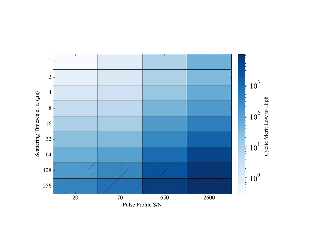
Figure 1: Quality of impulse response function recovery for simulated pulsars using the WDS algorithm (Section 5.1). Higher values in colorbar mean better quality of recovery. The values in each cell were originally goodness-of-fit metrics $\Delta$, then reassigned to cyclic merit values $m_{\rm cyc}$ (Equation 12), as described in Section 5.2. Values of $\tau_{\rm s}$ are in $\mu$s. Each cell corresponds to $>$60 simulations, with the color corresponding to the median $m_{\rm cyc}$ value. Simulations in the crosshatched region are those in which scintles are not resolved by the fixed number of radio frequency channels across the simulations performed here, in which case the recovered IRFs are broad one-sided exponentials. The simulations verify that the effectiveness of CS deconvolution is proportional to both pulse profile S/N and scattering timescale $\tau_{\rm s}$.

5 Results and Comparisons with Observations

Using the simulations, quality measurements, and theoretical cyclic merit from the previous two sections, we compare a suite of simulations to test the dependence of $m_{\rm cyc}$ on $\tau_{\rm s}$ and $S/N$. We also compare several observations to the theoretical cyclic merit predictions, establishing a fiducial metric for the reliability of routine deconvolution of the IISM.

5.1 Measuring the Simulated Cyclic Merit Relationship

Results from the simulations are summarized in Figure 1. Each cell in the grid corresponds to a combination of $\tau_{\rm s}$ and S/N ratio. The color scale corresponds to the logarithm of the $m_{\textrm{cyc}}$ values described in Section 3. The $\Delta$ values from each corresponding simulated and recovered IRF pair were calibrated to the theoretical $m_{\textrm{cyc}}$ values by the procedure to be described in this section, and then rescaled to arrive at the merit-based color scaling in Figure 1. Note that while the vertical axis shows $\tau_{\rm s}$ values that are powers of two, the $S/N$ values in the horizontal axis increase by a factor of $\sim$3.5 except from 70 to 2600 which increases by almost two of the logarithmic intervals. We did not simulate the missing middle column to save computing time; the gap is taken into account in our linear regression procedure.

For the B1937+21-like artificial pulsar used in the simulations (similar in period and in main pulse width, with no interpulse in simulations), we relate our goodness-of-fit metric $\Delta$ to $m_{\rm cyc}$ by:

$$\Delta={A}m_{\textrm{cyc}}^{-\mu}$$ (14)

because we expect an inversely monotonic relationship between $\Delta$ and $m_{\textrm{cyc}}$ across many orders of magnitude in $\tau_{\rm s}$ and $S/N$, but we do not know the details of how the two will correspond at low $m_{\textrm{cyc}}$, as discussed in Section 4.2. We assume $\mu$ is a constant with respect to $\tau_{\rm s}$ and $S/N$. Although we already have a theoretical expectation for how $m_{\textrm{cyc}}$ will depend on $\tau_{\rm s}$ and $S/N$ from Equation A11, we parameterize possible powerlaw dependencies as:

$$m_{\textrm{cyc}}\propto\tau_{\rm s}^{\beta}\left({\mathrm{S/N}}\right)^{\gamma}.$$ (15)

We are interested in verifying that the simulation results demonstrate that $\beta=1$ and $\gamma=1$, which would be consistent with the derivation in Appendix A. Re-writing this in logarithmic form, Equation 15 becomes:

$$\mathop{\log_{10}}{m_{\textrm{cyc}}}=\beta{\mathop{\log_{10}}{\tau_{\rm s}}}+\gamma\mathop{\log_{10}}{\left(\mathrm{S/N}\right)}+C$$ (16)

where $C$ is a constant derived from pulsar-specific parameters in Equation A11. We can then substitute Equation 14 into Equation 16 to obtain:

$$-\frac{1}{\mu}\mathop{\log_{10}}{\Delta}=\beta{\mathop{\log_{10}}{\tau_{\rm s}}}+\gamma\mathop{\log_{10}}{\left(\mathrm{S/N}\right)}+D$$ (17)

where $D$ depends on both $A$ and $C$. Proceeding, we note that because:

$$\mathop{\log_{10}}{\Delta}=-\mu\beta{\mathop{\log_{10}}{\tau_{\rm s}}}-\mu\gamma\mathop{\log_{10}}{\left(\mathrm{S/N}\right)}-\mu{D}$$ (18)

we cannot measure $\beta$ and $\gamma$ from the results of our simulations because each will be covariant with $\mu$. However, we can measure the ratio $\gamma/\beta$, which should be 1, by least-squares linear regression. This is equivalent to measuring the direction of the gradient of $\mathop{\log_{10}}{\Delta}$ but not its magnitude. Because we have derived $\beta=1$ and $\gamma=1$ in Appendix A, the gradient of $\Delta$ should point in the $(1,1)$ direction in $\mathop{\log_{10}}\tau$-$\mathop{\log_{10}}(\mathrm{S/N})$ space. We ignore the constant $\mu{D}$ in our fitting.

The distribution of the $\Delta$ values within each cell was approximately Gaussian. Across cells, the median $\Delta$ values appear approximately coplanar in Figure 1 by eye. An exception is the upper right cell which is a local minimum compared to the surrounding cell. We examined the individual input and output IRFs and found that because the S/N was very high in this region, most $\Delta$ values were very near zero. The statistical distribution of the $\Delta$ values was different from the apparently Gaussian distribution in other cells, most likely because the statistics are determined more by the numerical properties of the computational process than by the simulated IISM properties. In the following fit, we neglect this outlier upper-right cell.

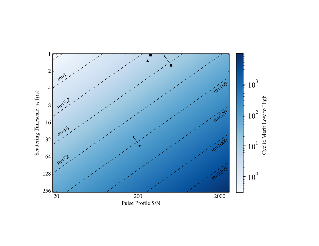
Figure 2: Theoretical quality of impulse response function recovery (Section 5.2) from Equation 12. Four examples of CS deconvolution on real pulsars are also shown: PSR J2317+1439 at 327 MHz (triangle), PSR B1937+21 at 430 MHz (star; from Walker et al. 2013), PSR J1713+0747 at 327 MHz (square), and PSR B1937+21 at 1410 MHz (circle). Of the four real pulsar examples, the upper three real pulsars did not successfully recover an IRF, which is consistent with their low cyclic merit ($m_{\rm cyc}$) values. The predicted cyclic merit values shown in the colorscale are for a generic pulsar with the period and equivalent width of PSR B1937+21, and the pulse profile shape of the PSR B1937+21 main pulse only. Pulsars J1713+0747 and J2317+1439 therefore have $m_{\rm cyc}$ values that differ slightly from those shown. The arrows next to both observations of PSR B1937+21 indicate that in reality, the interpulse reduces the cyclic merit by a factor of $\sim$2, resulting in three of the four observations with $m_{\rm cyc}<10$, those three which we also found to not regularly converge on a best-fit IRF. Note that a pulsar’s S/N is entirely dependent on the telescope sensitivity and on the folding time. Upcoming telescopes will move more pulsars to the right. Inclusion of significantly scattered pulsars not currently used in timing programs will further populate the bottom of the plot with high $m_{\rm cyc}$ pulsars.

A two-parameter unweighted linear regression of $\mathop{\log_{10}}{\Delta}$ with $\mathop{\log_{10}}{\tau_{\rm s}}$ and $\mathop{\log_{10}}{\mathrm{S/N}}$ yields slopes of $-\mu\beta=-1.86\pm 0.07$ and $-\mu\gamma=-1.92\pm 0.07$ respectively, with an $r^{2}$ regression statistic of 0.98. The slope ratio $\gamma/\beta$ is therefore $0.98\pm 0.05$. With these nearly coplanar values and the expected gradient direction, we compute the $m_{\rm cyc}$ values from Equation 12 for a B1937+21-like pulsar and assign those values to the cells, shown in the color scale of Figure 1.

The bottom crosshatched two rows of Figure 1 are those in which the scintles are not resolved, and in which, as a result, the success of the WDS algorithm in those cells is not representative of the full capability of the algorithm.

The radio frequency channel size here is 1 MHz$/2048=0.488$ kHz, which is held constant over all the simulations so that $\tau_{\rm s}$ and $S/N$ are the only variables changed. By Equation 1, for $\tau_{\rm s}=64\mathrm{\mu s}$, $\Delta\nu_{d}=2.5$ kHz, and we have $\sim$5 channels per scintle. At $\tau=128\mathrm{\mu s}$ we have 1 or 2 channels per scintle, making resolving the scintles difficult. Because the scintillation structure across radio frequency corresponds to the multiplicative noise structure in an IRF, unresolved scintles are equivalent to a one-sided exponential IRF with no additional structure. The situation of unresolved scintles often occurs when observing pulsars at radio frequencies $<100$ MHz; scattering timescales are measured by taking an intrinsic pulse shape derived from higher frequencies and convolving with one-sided exponentials until the model profiles match the data (Bansal et al. 2019). The crosshatched rows represent simulations with no IISM information gained over the method of successive convolutions with smooth, one-sided exponential IRFs. However, we are not aware of any reasons why WDS would perform poorly for the highly scattered pulsars represented in the bottom two rows of Figure 1 if we had used a greater number of channels. The slope ratio $\gamma/\beta$ for Figure 1, removing both the upper right outlier and the crosshatched cells, is $1.02\pm 0.08$ with an $r^{2}$ regression statistic of 0.97, consistent with the prediction from Equation 12. The S/N in Figure 1 is integrated over the band, not the single-channel S/N.

5.2 Comparisons of Figure-of-merit with Observations

In Figure 2, we show $m_{\rm cyc}$ predictions using, as in Figure 1, the period and main-pulse $W_{e}$ for PSR B1937+21 as representative quantities for a generic MSP. We then compare to data.

The observations used here, in addition to the 430 MHz data on PSR B1937+21 used in Demorest (2011) and Walker et al. (2013), were taken from three separate campaigns at Arecibo on pulsars PSR J1713+0747 (4.6 ms period) at 327 MHz, PSR B1937+21 (1.6 ms period) at 1.4 GHz, and PSR J2317+1439 (3.4 ms period) at 327 MHz. All three datasets were baseband. The PSR J1713+0747 data (AO P2627, PI Palliyaguru) were taken at 430 MHz on 19-Sep-2011 with Mock spectrometers as backend receivers and were 40 MHz wide in bandwidth, with a 10 MHz slice used for the deconvolution attempt. The PSR B1937+21 data (AO P2676, PI Dolch) were taken on 19-Sep-2012 and the PSR J2317+1439 data (AO P2824, PI Stinebring) were taken on 02-Aug-2013, both with the PUPPI backend (Puerto Rican Ultimate Pulsar Processing Instrument; DuPlain et al. 2008) with a 200 MHz and a 50 MHz bandwidth, respectively. Data were folded into cyclic spectra using the “–cyclic” option in the dspsr package (van Straten & Bailes 2011, Demorest 2011). The deconvolutions used 25 MHz of the available bandwidth unless stated otherwise, which simplified the dataset because of band gaps between channels. The cyclic spectrum was accumulated in integrations such that the duration of each integration was less than the diffractive timescale, so that the IRF would be stable throughout each integration. The S/N of each data set was high enough that scintles were visually apparent in dynamic spectra formed from the data. For most subintegrations of data, the WDS procedure was applied and no converging IRF was found. We attempted a number of different starting conditions, varying the shift in phase between input profile and the measured profile, but in none of these cases did the algorithm yield a coherent solution. The same stopping and convergence criteria were used on both the data and the simulations. We found one well-fitting IRF in a subintegration of the PSR B1937+21 data at 1.5 GHz, but based on the cyclic merit values in Figure 1, we expect an occasional convergence by chance that may nor may not represent the true underlying state of the IISM during that subintegration.

The examples of deconvolution attempts on real data are plotted in Figure 2 along with the converging example from (Demorest 2011) and (Walker et al. 2013). The $S/N$ values for the data new to this paper were computed using a 25 MHz bandwidth. The three non-converging examples are in a region of $\tau_{\rm s}$-$S/N$ space predicted to have poorer deconvolution quality than the converging example by an order of magnitude. The $\tau_{\rm s}$ values and each pulsar’s measured frequency powerlaw used here are from the NANOGrav 12.5-year dataset (Turner et al. 2020), unless otherwise stated. We recognize these values are representative of highly variable IISM structures along a pulsar’s line-of-sight (the variability motivating CS deconvolution) but many reported values in the literature differ. The $a_{k}$ values (Equation 12) used were also from the NANOGrav 12.5-year dataset (Alam et al. 2021a). The $m_{\rm cyc}$ value for PSR J1713+0747 at 430 MHz ($\tau=1.0\mathrm{\mu s}$; $S/N$ = 285) was 4.3. For PSR B1937+21 at 1.4 GHz ($\tau_{\rm s}=1.6\mathrm{\mu s}$; S/N = 506), $m_{\rm cyc}=12.2$. PSR B1937+21 at 430 MHz had $m_{\rm cyc}=125$ ($\tau_{\rm s}=40\mathrm{\mu s}$; $S/N$ = 209, Walker et al. 2013, Demorest 2011, using the $-3.66$ frequency powerlaw dependence of $\tau_{\rm s}$ in Ramachandran et al. 2006 at a frequency of 1273 MHz where our baseband observations were located). Finally, PSR J2317+1439 at 327 MHz ($\tau_{\rm s}=1.3\mathrm{\mu s}$; $S/N$ = 262) had $m_{\rm cyc}=5.1$.

In reality, these four pulsar observations will correspond to different colorscales in Figure 2 because they have different values of $P$, $W$, and $\sum_{k}k^{2}a_{k}$ in Equation 12, whereas the colorscale of Figure 1 is based on PSR B1937+21. The $m_{\rm cyc}$ values for PSR J1713+0747 and PSR J2317+1439 are slightly higher and lower respectively due to the sharper pulse of the second producing more $a_{k}$ terms in Equation 12. Our stated $m_{\rm cyc}$ values for PSR B1937+21 are greater than the true $m_{\rm cyc}$ values by a factor of $\sim$2 because the presence of the interpulse reduces $\sum_{k}k^{2}a_{k}$ in Equation 12. The arrows in Figure 2 point to the true $m_{\rm cyc}$ contour line where the two PSR B1937+21 observations should reside. For PSR B1937+21 at 430 MHz (Walker et al. 2013), the actual $m_{\rm cyc}$ value is 66. Because our simulations were done on a single-component pulse profile representing a generic MSP, in Figure 2 we still plot the $m_{\rm cyc}$ value from PSR B1937+21’s main component $m_{\rm cyc}$ only. The results remain consistent with the concept of $m_{\rm cyc}$ as a unitless detection “signal” of a scattering tail. Taking the interpulse into account, the three unsuccessful CS deconvolution attempts have $m_{\rm cyc}<10$ and the successful attempt has $m_{\rm cyc}=66$, which is why we use $m_{\rm cyc}=10$ as an absolute minimum requirement for CS-enhanced pulsar timing in Section 6.

The predictions in Figure 2, verified by the simulations in Figure 1, suggest that despite the large amount of phase-wrapping, a pulsar in the bottom-left of Figure 2 – highly scattered but low S/N – could be successfully IISM-deconvolved. The large amount of scattering would mean a high duty cycle in the scattered pulse profile. The de-scattered profile in such a case would both be scattering-corrected in terms of its TOAs (by eliminating variations in the IRF), as well as turned into a better precision-timed pulsar with its low-duty-cycle unscattered pulse profile. However, this possibility would need case-by-case evaluation: as we move toward lower frequencies, $\tau_{s}$ increases, but the diffractive timescale decreases (Cordes & Shannon 2010), limiting the maximum integration time. A smaller $\Delta\nu_{d}$ also lowers the S/N per scintle. A correct application of the figure-of-merit (Figure 2) to pulsar observations should take these considerations into account.

A more detailed simulation will be necessary to evaluate the following cases, which depend on the pulsar and the observation in question:

• If the pulsar flux becomes comparable to the telescope’s system equivalent flux-density, then the on-pulse noise (due to the pulsar’s own AMN) will significantly exceed the off-pulse noise, unlike our simulations which assume the same noise properties across all phases of the profile.

• If the number of pulses averaged to obtain a cyclic spectrum is too low, then the effects of pulse phase jitter will be important (Lam et al. 2019), and the correlations between ${S_{E}}(\nu,\alpha_{k})$ bins in the cyclic spectrum array will become significant. Pulse phase jitter - the intrinsic white-noise distributed TOAs of single pulses - cannot be reduced by telescope sensitivity, as the TOA uncertainties are intrinsic to the pulsar. The TOA uncertainties can be reduced by longer integration times, but this is not helpful for mitigating scattering in real time, with the longest integration time on the order of a diffractive timescale. For highly scattered pulsars, the diffractive timescale may in some cases become so low that the necessary S/N for CS deconvolution is not possible.

As long as a particular pulsar observation is free of the above two properties, Figure 2 can be expected to reasonably predict whether CS deconvolution is feasible.

Figure 2 does not imply that CS is totally inapplicable to pulsar observations with $m_{\rm cyc}<10$. Even if deconvolution is infeasible, a cyclic spectrum still contains a detailed measurement of the presence of scattering, in addition to providing an extremely fine frequency resolution. In some cases, CS deconvolution may be possible even when $m_{\rm cyc}<10$. What we have tested here is a straightforward, untailored application of the WDS algorithm. In practice, well-measured long-term PBFs for particular pulsars could serve as ideal initial conditions, instead of the delta functions used here. An ideal frequency binning could also change the behavior of the algorithm. Such approaches would model a line-of-sight and repeatedly update that model, much in the same way that pulsar timing models are repeatedly updated. The cyclic merit concept, then, must be understood as a measure of how reliably the WDS algorithm can quickly and routinely deconvolve, as in a real-time data processing pipeline.

The improvement in timing precision for a simulated Galactic MSP population from the PsrPopPy code observed with the Green Bank Telescope’s ultrawide bandwidth (UWB) receiver, currently under construction. Cyclic spectroscopy deconvolution has the potential to double the number of PTA-quality MSPs with $\sigma_{\rm TOA}<1\;\mathrm{\mu s}$ at the GBT using the UWB receiver. The (blue) “Always PTA-quality” MSPs have similar properties to current NANOGrav pulsars. The (green) “PTA-quality only w/CS” are those MSPs that could be included in the NANOGrav PTA because of the improved UWB sensitivity.

The same simulated pulsars are plotted as in Figure 5.2, but with the colorscale representing the $\tau_{\rm s}$ value of each simulated pulsar. The pulsars with the greatest timing improvements tend to be those with the longest scattering tails, but the majority of the “PTA-quality only w/CS” pulsars have scattering tails with $\tau_{\rm s}$ values of $\sim 10-100\mathrm{\mu s}$, in accordance with Figure 1. The dotted lines correspond to the classification regions from Figure 5.2.

6 Predictions for Pulsar Populations

Figure 2 suggests that many pulsars in addition to PSR B1937+21 could have high $m_{\rm cyc}$ values, most of which are not currently included in PTAs. We estimate the number of pulsars that could be successfully deconvolved in a future version of Figure 2 using the example of the GBT ultrawide bandwidth (UWB) receiver currently under construction. The GBT’s UWB receiver, similar to the UWB receiver developed by CSIRO for the Parkes Radio Telescope, spans the 0.7–4 GHz range.

We simulated the full Galactic MSP population using the PsrPopPy library (Bates et al. 2014) with the expected UWB system temperatures and gains across the bandwidth, ${\mathcal{T}_{\rm obs}}$ = 15 min (corresponding to typical DISS timescales), and assuming a Gaussian pulse profile shape. The pulsars had the requirement that $\tau_{\rm s}<P/2$, because more highly scattered pulsars are unlikely to be detected in untargeted surveys. We also assumed that any pulsar with a large value of $m_{\rm cyc}$ would have sufficiently high S/N to be detected in future surveys. Finally, we calculated the rms timing residual, $\sigma_{\rm TOA}$, expected (Lam et al. 2018) for two cases: 1) traditional processing, in which scattering is not mitigated for any MSP, and 2) CS processing, in which we set $\tau_{\rm s}=0$ for any MSP with $m_{\rm cyc}\geq 10$ at 0.8 GHz (equivalent to completely mitigating all IISM noise at a typical NANOGrav timing frequency). We used $m_{\rm cyc,full}$ from Equation A12, because we assume that the high-resolution dynamic spectra from CS will resolve scintles, enabling the usage of a bandwidth over which we would measure $m_{\rm cyc}$ that varies with $\tau_{\rm s}$. The timing rms due to variations in the IRF is assumed to be 50% of $\tau_{\rm s}$ (Lam et al. 2018). The quantity $\sigma_{\rm TOA}$ also includes the rms from timing residuals from phenomena such as long-term DM variations.

The results are shown in Figure 5.2. We find that $\sim$40 MSPs that would otherwise not be of PTA-quality (i.e., $\sigma_{\rm TOA}>1$ $\mathrm{\mu s}$; the pulsars shown in green) become PTA-quality with the use of CS and the GBT UWB receiver. This is compared to 45 MSPs that are always of PTA-quality using the UWB receiver, even without the use of CS (the pulsars shown in blue). These population simulations suggest that CS deconvolution could double the number of PTA-quality MSPs, using the example of the GBT as one of many telescopes undergoing a receiver upgrade. We also find that the mean $\sigma_{\rm TOA}$ improves from $\sim$45 $\mathrm{\mu s}$ without CS to $\sim$ 2$\mathrm{\mu s}$ with CS. We note that this simulated population includes pulsars similar to current NANOGrav pulsars as well as pulsars either not yet discovered or not yet included as PTA pulsars due to high scattering and/or low S/N. The off-diagonal blue points in Figure 5.2 likely represent pulsars not yet discovered (see Section 7). The blue points along the diagonal represent a population similar to NANOGrav pulsars, both discovered and yet-to-be-discovered, for which CS deconvolution does not improve timing.

Several caveats about the cyclic merit values used to create Figure 5.2 bear mentioning. Because detailed profile information is difficult to extract from the population simulations, we only use the $a_{1}$ term in Equation A12, which may underestimate the cyclic merit of each pulsar in the simulated population, and thus the number that would improve to PTA quality. On the other hand, we also assumed that $m_{\rm cyc}>10$ implies complete scattering removal; the true degree of removal will depend on the details of the timing pipeline used (see Section 7). The threshold $m_{\rm cyc}$ might in practice also be larger than 10; all we can say definitively is that $m_{\rm cyc}\gg 1$ for scattering removal (with motivation for a threshold of 10 from our data in Section 5.2). Although we calculated $\sigma_{\rm TOA}$ at 0.8 GHz, $m_{\rm cyc}$ may also need to be $>$10 at more than one frequency across the UWB receiver’s bandwidth in order to improve timing precision, possibly reducing the number of pulsars correctable to PTA-quality. As these caveats are difficult to quantify, we do not attempt to refine them further in this work. At the very least, the “PTA-quality only with CS” designation in Figure 5.2 suggests a possible population of pulsars with good timing quality that has yet to be exploited. The artificial pulsars with a factor of $\sim$100 improvement are not known PTA pulsars that would improve by such a significant factor (note the smaller improvement factors for the “Always PTA-quality” pulsars). The pulsars with a factor of $\sim$100 improvement in $\sigma_{\rm TOA}$ are rather those that in the absence of CS deconvolution would likely have never had a full timing solution prior to CS pulse-sharpening. The improvements in Figure 5.2 must be understood with this last consideration especially in mind.

Figures 5.2, 6, and 6 show some interesting properties of the predicted populations. Pulsars with the largest improvement (Figure 5.2) tend to be those with large $\tau_{\rm s}$ values but also narrow intrinsic pulse widths. The probability density function of pulse widths is shown in Figure 6. We measured width by $W_{\rm eff}/P$, where $1/W_{\rm eff}$ is the mean-squared derivative of the pulse profile (Downs & Reichley 1983, Lam et al. 2016a). The distribution in Figure 6 tends toward narrower pulse widths for the “PTA-quality only w/CS” sub-population, suggesting that their narrow intrinsic widths in particular will enable better timing. While these have notably narrow pulse widths, the lognormal distribution from which widths are drawn matches the width distribution from the NANOGrav 12.5-year dataset. As Figure 6 shows, the distribution of the “PTA-quality only w/CS” pulsars in Galactic coordinates tends toward the Galactic center, with the highest timing residual rms improvements corresponding to the most distant pulsars. Bright, intrinsically narrow, and highly scattered pulsars may very well acquire low timing rms values by means of CS.

Probability density functions of the pulse sharpness measurements, $W_{\rm eff}/P$, for the intrinsic (unscattered) pulse shapes from all the simulated pulsars in Figure 5.2. Both the “PTA-quality only w/CS” and the entire population of simulated pulsars have sharper intrinsic pulses, enabling good timing quality if CS deconvolution is applied.

Galactic spatial distribution of simulated pulsar set from Figure 5.2. The solar system is the black circled dot. Those pulsars acquiring PTA-quality after CS deconvolution tend to be more distant than those PTA pulsars with no or small timing improvements after CS deconvolution. The small subset with extremely large timing improvements are the most distant of the “PTA-quality only w/CS” pulsars, consistent with their significant scattering from Figure 6.

7 Conclusions and Next Steps

To reiterate, we expect several possible CS deconvolution benefits for PTA pulsars:

• Improved timing precision of current PTA pulsars through scattering correction at some or all radio frequencies across a wide bandwidth. For any particular pulsar currently with PTA-quality timing precision, the timing correction may be one of many small second-order corrections, but at least for some current PTA pulsars, a S/N improvement with a new receiver and/or telescope may enable a more significant correction (blue points in Figure 5.2, allowing a movement to the right in Figure 2).

• Future pulsar discoveries, likely to be more distant and highly scattered, that can become PTA-quality through removal of scattering variations. CS deconvolution also applies to known pulsars currently with low timing precision, IISM-deconvolved to have PTA-quality timing precision.

• Enabling observations at lower frequencies not presently used for pulsar timing where pulsars are intrinsically brighter, given the approximate relationship $\tau_{\rm s}\propto\nu^{-4.4}$. Low-frequency telescopes and instruments could become more important for pulsar timing.

A procedure for using CS to improve pulsar timing precision is described in Palliyaguru et al. (2015). The approach uses a timing model, fitting the WDS-recovered IRF with a one-sided exponential. The results are encouraging, although as the paper states, work still remains to implement a full pulse-sharpening procedure. Our present work demonstrates that the pulse-sharpening itself will likely be effective if $m_{\rm cyc}>10$ for a particular pulsar; demonstration of a full timing pipeline involving CS deconvolution is a work in progress.

Several additional procedures will need to be incorporated into a full CS timing pipeline. Scattering correction methods are most relevant to low radio frequencies. Because high timing precision requires a DM measurement, which in turn requires high precision across a wide range of frequencies, scattering variations (and thus the changing IRF) would be highly covariant with any DM variations. If scattering variations are significant enough, then scattering delays can be partially absorbed into the DM measurement. Such an effect would, of course, represent a real source of error not otherwise taken into account, and CS would be useful for characterizing that error, but improved timing precision is not guaranteed. If scattering is high enough, then DM measurements could become contaminated (Levin et al. 2016). For most pulsars, the scintillation timescale, the timescale on which IRF realizations change, is significantly less than the typical timescale for DM variations, reducing the possibility of covariance.

For PSR B1937+21, CS deconvolution is unsuccessful only for the 1.4 GHz data presented here; at 430 MHz, Demorest (2011) and Walker et al. (2013) successfully obtained an IRF. Being heavily subject to red noise (Kaspi et al. 1994, Lam et al. 2017, Lam et al. 2016b), PSR B1937+21 is not a useful contributor for most expected GW signals, given the necessity for stability on decades’ timescales. It remains included in the list of routinely timed NANOGrav pulsars in order to compare arrival times between telescopes, and because of its very high short-term timing precision, making it sensitive to burst sources on timescales of approximately months (Finn & Lommen 2010). Such bursts could arise from nearby individual supermassive black hole binaries in highly elliptical orbits. PSR B1937+21’s short-term GW sensitivity could be improved by routine CS deconvolution.

In the case of NANOGrav, the PTA’s pulsars typically have $\tau_{\rm s}$ values $<$10 $\mu$s (Levin et al. 2016, Turner et al. 2020), corresponding to low cyclic merit values. This is not surprising because the pulsars were selected for high timing precision. CS, however, remains an effective technique for obtaining extremely fine frequency resolution, and should still be performed as a routine data product. Finer frequency resolution helps to better excise radio frequency interference (RFI) using the RFI itself as the cyclostationary “signal”, and can also provide higher frequency-resolution dynamic spectra, either for IISM studies or as a diagnostic tool for timing. For example, highly scattered epochs could be measured with fine-resolution cyclic periodograms (as demonstrated by Archibald et al. 2014) and then appropriately down-weighted in a GW detection pipeline. Preliminary high-resolution dynamic spectra using CS were also created as part of the IPTA’s 24-hour global campaign on PSR J1713+0747 (Dolch et al. 2014).

The practical difficulty of CS as a routine data product is the large volume of baseband data. Real-time CS backend receivers are currently being pursued in order to create cyclic spectra and/or IISM-deconvolved timing data as a direct data product, so that baseband data will not need to be saved for post-processing.

Within the current 12.5-year NANOGrav dataset (Alam et al. 2021a, Alam et al. 2021b), PSR J1903+0327 is an example of a high-DM NANOGrav pulsar that would likely benefit from such a routine procedure. Using NANOGrav 12.5-year dataset profiles, values from the ATNF pulsar catalog, and the assumption of increasing flux at low frequencies with a $-1.4$ powerlaw dependence, we estimate $m_{\rm cyc}$ $\sim$4 at 820 MHz for PSR J1903+0327. The true scattering timescale has not yet been estimated from resolved scintles. Improved frequency resolution with CS and/or improved telescope sensitivity could show a higher merit value. The calculation assumes an the AO sensitivity, but given the improved system temperature of the UWB receiver, this is still a pulsar worth exploring with the upgraded GBT. Other distant, high-DM pulsars for which good non-NANOGrav timing solutions already exist could be added to the array. However, these added pulsars must not be scattered so highly that low-frequency scintles are unresolvable (Cordes & Shannon 2010); in the NANOGrav 12.5-year dataset scattering measurements (Turner et al. 2020), all pulsars either have $\tau_{\rm s}<1\mathrm{\mu s}$ at 820 MHz or have unresolvable scintles at the observed frequencies. Routine, fine-frequency dynamic spectra from CS may resolve currently unresolved scintles for PTA pulsars such as PSR J1903+0327, after which, CS pulse-sharpening may be applicable.

Other possible benefits of CS deconvolution are likely to occur for other telescopes not yet mentioned (Dolch 2019). The Canadian HI Mapping Experiment (CHIME; Bandura et al. 2014, Ng et al. 2020), although primarily searching for high-redshift baryon acoustic oscillations, observes transiting pulsars daily from 400 MHz to 800 MHz, typical frequencies in which $\tau_{\rm s}$ is large enough that CS deconvolution could be successfully applied on many pulsars. Combined with the high cadence, CHIME’s sensitivity to short-timescale GW bursts would improve with routine CS deconvolution. The telescope is not steerable, but a pulsar-specialized backend receiver extracts pulsar timing data from the large volume of information constantly obtained at the instrument’s many receivers (CHIME/Pulsar Collaboration et al. 2020). CHIME can obtain high-time-sampled, low-frequency data as well as make discoveries of pulsars in its declination range. The future Square Kilometer Array, and the current pathfinders - Australian Square Kilometre Array Pathfinder (ASKAP; (Johnston et al. 2009)) and MeerKAT (Gibbon et al. 2013) - are expected to discover a significant fraction of all the visible pulsars in the Galaxy (Cordes et al. 2004). A Next-Generation Very-Large Array (ngVLA; NANOGrav Collaboration 2018) has also been proposed for the northern hemisphere. Both telescopes are expected to have a factor of $\sim$10 improvement in sensitivity over AO, improving the $m_{\rm cyc}$ for many currently fainter pulsars. As already discussed in Section 6, the GBT UWB receiver will enable simultaneous, highly sensitive pulsar observations across 3.3 GHz. In Figure 2, these future telescopes or upgrades would move the example pulsars at least an order of magnitude to the right on the diagram. As a low-$\sigma_{\rm TOA}$ example, PSR J1713+0747 would be located in the upper-right region of the plot instead of the upper left. While CS deconvolution would require many computing nodes across a large bandwidth, such computing resources will be a part of the full SKA or ngVLA. With these telescopes, many pulsars will have S/N similar to that of PSR B1937+21 now. These changes could heavily populate the diagnostic diagram in this paper with pulsars that are high S/N enough and/or highly scattered enough for feasible routine CS deconvolution.

In addition to the successful application of CS to LOFAR data (Archibald et al. 2014), other low-frequency radio telescopes (e.g., 200 MHz and below) could benefit from routine CS data products, for the sake of both fine channelization data products and for deconvolution. While these frequencies do not usually allow for precision timing, the significant scattering tails present could be utilized vis-a-vis CS deconvolution to significant improve timing precision, or to arrive at stable timing solutions otherwise unavailable before CS deconvolution. The Long-Wavelength Array (LWA), recently expanded to two stations with a significant sensitivity increase, is a relevant example. The LWA is already monitoring many pulsars (Stovall et al. 2015), several of which are currently NANOGrav MSPs. Future low-frequency telescopes such as SKA-low in the southern hemisphere and the proposed LWA-Swarm telescope (Dowell & Taylor 2018, Taylor et al. 2019) may have sensitivities for a significant S/N boost in Figure 2. The Expanded LWA (ELWA; Taylor et al. 2017, Ruan et al. 2020) already uses recently installed 50–80 MHz dipoles on the VLA together with the two LWA stations. Even if low-frequency timing does not become feasible, these low-frequency telescopes aided with CS can complement timing observations with DM measurements and with monitoring of CS-resolved secondary spectra (the parabolic 2D FTs of dynamic spectra containing scattering structure information) as done with PSR B1937+21 in Walker et al. (2013). Finally, CS has been successfully applied to data from the VLA Low Band Ionospheric and Transient Experiment (VLITE; Polisensky et al. 2016) project in order to provide very high-frequency resolution for RFI excision (M. Kerr, private communication). For the transient search aspect of VLITE, the improved frequency resolution of periodic RFI (Demorest 2011), and therefore the improved quality of RFI excision, could aid the search for fast radio bursts or other radio transients. The Breakthrough Listen project, along these lines, has searched for technosignature periodicities in association with FRBs (Price et al. 2019), by creating cyclic spectra, shifting at multiples of small time intervals and seeing if power appears in harmonics of a particular period. Beyond transient radio astronomy, as in radio spectral line observations, routine CS would also help excise RFI.

CS may also serve as an important pulsar searching tool. The presence of scattering in a CS phase slope could serve as an additional pulsar searching metric, along with trial DMs and periods, for an astrophysically pulsating signal. Searches near the highly scattered Galactic center might particularly benefit from CS as a routine and/or real-time data product.

8 Acknowledgments

We thank the referee for the many helpful suggestions that have been incorporated into this paper. We thank J. M. Cordes, T. T. Pennucci, M. Kerr, and the NANOGrav collaboration for helpful discussions and suggestions, the Noise Budget Working Group in particular. We thank the AO staff for their assistance during the observations reported in this work, in particular P. Perillat, J. S. Deneva, H. Hernandez, and the telescope operators. We are grateful for the use of the Bowser computing cluster at WVU with the assistance of N. E. Garver-Daniels. From Hillsdale College, TD gratefully acknowledges computing resources from the Department of Physics, summer leave funds, and professional development funds for conducting this research. The authors were partially supported through the National Science Foundation (NSF) PIRE program award number 0968296. Members of the NANOGrav Collaboration (TD, DS, RL, PD, ML, MM) acknowledge support from the NSF Physics Frontiers Center (PFC) award number 1430284. TD acknowledges NANOGrav seed-funding for meetings where this research was conducted. AO is a facility of the NSF operated under cooperative agreement by UCF in alliance with Yang Enterprises, Inc. and Universidad Metropolitana. The Green Bank Observatory (GBO) is a facility of the NSF operated under cooperative agreement by Associated Universities, Inc. The GBT UWB receiver project is funded in part by the Gordon and Betty Moore Foundation through Grant GBMF7576 to Associated Universities Inc. to support the work of the GBO and the NANOGrav PFC. TD and MTL are supported by an NSF Astronomy and Astrophysics Grant (AAG) award number 2009468. This work made use of NASA’s ADS and the arXiv.org preprint service.

Appendix A Derivation of the Cyclic Merit

According to Equation 10, the phase of the cyclic spectrum has two contributions: one term induced by the derivative of the phase of the IISM transfer function and the other intrinsic to the pulse profile. By the shift theorem in Fourier analysis, a translation in the time domain induces a phase slope in the frequency domain. Since the time-domain impulse response function is characterised by a delay $\tau_{\rm s}$, we can estimate the phase derivative of the transfer function by $-2\pi\tau_{\textrm{s}}$,

$$\Phi_{S_{E}}(\nu,\alpha_{k}) =\frac{k}{P}\frac{\textrm{d}\Phi_{H}}{\textrm{d}\nu}+\phi_{S_{x}}(\alpha_{k})$$ (A1)

$$\approx-2\pi\frac{k\tau_{\textrm{s}}}{P}+\phi_{S_{x}}(\alpha_{k})$$ (A2)

$$\approx k\,b+\phi_{S_{x}}(\alpha_{k}),$$ (A3)

where $b=2\pi\tau_{\rm{s}}/P$ is the average cyclic phase slope, also equal to the expected phase at $k=1$.

The spectrum of the intrinsic pulse profile can be determined accurately by the WDS algorithm, since the Hessian is diagonal with respect to the set of parameters describing the profile (Walker et al. 2013). Hence, in general, the second term in Equation A3 does not complicate the phase retrieval process. At larger modulation frequencies, the CS amplitude is lost to the noise as in Figure 2.2 near $\alpha_{k}$ = 40, which causes a transition to incoherence in phase as in Figure 3.1. We can estimate the phase noise in a cyclic spectrum at the $k^{th}$ harmonic to be

$$\Delta\Phi_{k}\equiv\sigma_{\textrm{noise}}/{A_{k}}$$ (A4)

where $A_{k}$ is the frequency-averaged amplitude of the cyclic spectrum at harmonic $\alpha_{k}$. By a weighted linear fit, the phase slope $b$ can be estimated by

$$b=\frac{1}{\Delta_{w}}\sum_{k}{w_{k}\,k\,\Phi_{E}(k)},$$ (A5)

where the least-square weights are $w_{k}=1/[\delta\Phi_{E}(k)]^{2}$, and $\Delta_{w}\equiv\sum_{k}w_{k}\,k^{2}$ does not depend on the measured $\Phi_{E}(k)$ values. Then, the uncertainty in the phase slope $b$ is

$$\delta b =\frac{1}{\Delta_{w}}\sqrt{\sum_{k}{w_{k}^{2}\,k^{2}\,[\delta\Phi_{E}(k)]^{2}}}$$ (A6)

$$=\frac{1}{\Delta_{w}}\sqrt{\sum_{k}\frac{k^{2}}{[\delta\Phi_{E}(k)]^{2}}},$$ (A7)

where all the sums are from 1 to $N_{\rm max}/2+1$ and where $N_{\rm max}$ is the number of time samples in the folded profile. This can be further simplified by expressing the uncertainty of the cyclic spectrum phase in terms of observational parameters from the radiometer equation:

$$\delta\Phi_{E}(k)\approx\Delta\Phi_{k}=\frac{\Delta\Phi_{0}}{a_{k}} =\frac{1}{a_{k}}\frac{T_{\rm sys}}{gS_{0}\sqrt{B{\mathcal{T}_{\rm obs}}}}.$$ (A8)

Here, $T_{\rm sys}$ is the system temperature, $g$ is the telescope gain (units: K/Jy), $S_{0}$ is the pulsar continuum flux (single polarization), $B$ is the bandwidth over which the phase information is integrated (ideally channelized to the diffractive bandwidth, $\Delta\nu_{d}$), and $\mathcal{T}_{\rm obs}$ is the observing time in the integration. Taken together, this allows us to define a quality metric, the cyclic merit, for cyclic spectroscopy phase retrieval, which we express as the signal-to-noise ratio of the cyclic spectrum phase

$$m_{\rm cyc}=\frac{b}{\delta b}=\frac{2\pi\tau_{\rm s}}{P}\frac{gS_{0}}{T_{\rm sys}}\sqrt{B{\mathcal{T}_{\rm obs}}\sum_{k}k^{2}a_{k}}.$$ (A9)

The above metric can then be written in terms of the folded pulse profile signal-to-noise ratio $S/N$

$$m_{\rm cyc}=\frac{2\pi\tau_{\rm s}W_{e}}{P^{2}}(S/N)\sqrt{\sum_{k}k^{2}a_{k}},$$ (A10)

where $W_{e}$ is the equivalent width of the pulse profile, and

$$(S/N)\equiv\frac{gS_{0}}{T_{\rm sys}}\frac{P}{W_{e}}\sqrt{B{\mathcal{T}_{\rm obs}\left(\frac{W_{e}}{P}\right)}}=\frac{gS_{0}}{T_{\rm sys}}\sqrt{B{\mathcal{T}_{\rm obs}\left(\frac{P}{W_{e}}\right)}}.$$ (A11)

Here we have assumed that the profile has been smoothed to a time resolution of $W_{e}$ for an optimal trade-off between pulse sharpness and $S/N$. In principle, the smoothing should be done to a time resolution of the sharpness width, $W_{s}\equiv\int{dt|U^{\prime}(t)|^{2}}$, where $U(t)$ is a unit amplitude average pulse profile, and the prime indicates a time derivative (Cordes & Shannon 2010). In practice, the quantitative difference between $W_{e}$ and $W_{s}$ is expected to be small for realistic pulse profiles.

Equation A9 is the cyclic merit for determining the average phase slope, which is a useful estimator of $\tau_{s}$. If a full reconstruction of the transfer function is required, we must estimate the cyclic spectrum phase over a diffractive bandwidth. This requires setting $B=\Delta\nu_{d}\approx 1/(2\pi\tau_{\rm s})$ in Equation A9 from which we obtain a cyclic merit for a full reconstruction of the transfer function

$$m_{\rm cyc,full}=\frac{gS_{0}}{PT_{\rm sys}}\sqrt{{2\pi\tau_{s}\mathcal{T}_{\rm obs}}\sum_{k}k^{2}a_{k}},$$ (A12)

where we see a square-root dependence on the scattering delay.

References

- Abbott et al. (2016) Abbott, B. P., Abbott, R., Abbott, T. D., et al. 2016, Physical Review Letters, 116, 061102, doi: 10.1103/PhysRevLett.116.061102
- Alam et al. (2021a) Alam, M. F., Arzoumanian, Z., Baker, P. T., et al. 2021a, ApJS, 252, 4, doi: 10.3847/1538-4365/abc6a0
- Alam et al. (2021b) —. 2021b, ApJS, 252, 5, doi: 10.3847/1538-4365/abc6a1
- Antoni (2007) Antoni, J. 2007, Mechanical Systems and Signal Processing, 21, 597, doi: 10.1016/j.ymssp.2006.08.007
- Archibald et al. (2014) Archibald, A. M., Kondratiev, V. I., Hessels, J. W. T., & Stinebring, D. R. 2014, ApJ, 790, L22, doi: 10.1088/2041-8205/790/2/L22
- Arzoumanian et al. (2018) Arzoumanian, Z., Baker, P. T., Brazier, A., et al. 2018, ApJ, 859, 47, doi: 10.3847/1538-4357/aabd3b
- Bandura et al. (2014) Bandura, K., Addison, G. E., Amiri, M., et al. 2014, in Society of Photo-Optical Instrumentation Engineers (SPIE) Conference Series, Vol. 9145, Society of Photo-Optical Instrumentation Engineers (SPIE) Conference Series, 22, doi: 10.1117/12.2054950
- Bansal et al. (2019) Bansal, K., Taylor, G. B., Stovall, K., & Dowell, J. 2019, The Astrophysical Journal, 875, 146, doi: 10.3847/1538-4357/ab0d8f
- Bates et al. (2014) Bates, S. D., Lorimer, D. R., Rane, A., & Swiggum, J. 2014, MNRAS, 439, 2893, doi: 10.1093/mnras/stu157
- Bhat et al. (2004) Bhat, N. D. R., Cordes, J. M., Camilo, F., Nice, D. J., & Lorimer, D. R. 2004, ApJ, 605, 759, doi: 10.1086/382680
- CHIME/Pulsar Collaboration et al. (2020) CHIME/Pulsar Collaboration, Amiri, M., Bandura, K. M., et al. 2020, arXiv e-prints, arXiv:2008.05681. https://arxiv.org/abs/2008.05681
- Coles et al. (2010) Coles, W. A., Rickett, B. J., Gao, J. J., Hobbs, G., & Verbiest, J. P. W. 2010, ApJ, 717, 1206, doi: 10.1088/0004-637X/717/2/1206
- Cordes et al. (2004) Cordes, J. M., Kramer, M., Lazio, T. J. W., et al. 2004, New A Rev., 48, 1413, doi: 10.1016/j.newar.2004.09.040
- Cordes et al. (2006) Cordes, J. M., Rickett, B. J., Stinebring, D. R., & Coles, W. A. 2006, ApJ, 637, 346, doi: 10.1086/498332
- Cordes & Shannon (2010) Cordes, J. M., & Shannon, R. M. 2010, ArXiv e-prints. https://arxiv.org/abs/1010.3785
- Cordes et al. (2016) Cordes, J. M., Shannon, R. M., & Stinebring, D. R. 2016, ApJ, 817, 16, doi: 10.3847/0004-637X/817/1/16
- Demorest (2011) Demorest, P. B. 2011, MNRAS, 416, 2821, doi: 10.1111/j.1365-2966.2011.19230.x
- Detweiler (1979) Detweiler, S. 1979, ApJ, 234, 1100, doi: 10.1086/157593
- Dolch (2019) Dolch, T. 2019, in 2019 United States National Committee of URSI National Radio Science Meeting (USNC-URSI NRSM), 1–2
- Dolch et al. (2014) Dolch, T., Lam, M. T., Cordes, J., et al. 2014, ApJ, 794, 21, doi: 10.1088/0004-637X/794/1/21
- Dolch et al. (2018) Dolch, T., NANOGrav Collaboration, Chatterjee, S., et al. 2018, in Journal of Physics Conference Series, Vol. 957, Journal of Physics Conference Series, 012007, doi: 10.1088/1742-6596/957/1/012007
- Dowell & Taylor (2018) Dowell, J., & Taylor, G. B. 2018, Journal of Astronomical Instrumentation, 7, 1850006, doi: 10.1142/S225117171850006X
- Downs & Reichley (1983) Downs, G. S., & Reichley, P. E. 1983, ApJS, 53, 169, doi: 10.1086/190890
- DuPlain et al. (2008) DuPlain, R., Benson, J., & Sessoms, E. 2008, in Society of Photo-Optical Instrumentation Engineers (SPIE) Conference Series, Vol. 7019, Society of Photo-Optical Instrumentation Engineers (SPIE) Conference Series, 1, doi: 10.1117/12.789402
- Finn & Lommen (2010) Finn, L. S., & Lommen, A. N. 2010, ApJ, 718, 1400, doi: 10.1088/0004-637X/718/2/1400
- Foster & Backer (1990) Foster, R. S., & Backer, D. C. 1990, ApJ, 361, 300, doi: 10.1086/169195
- Gardner (1991) Gardner, W. A. 1991, IEEE Signal Processing Magazine, 8, 14, doi: 10.1109/79.81007
- Geyer & Karastergiou (2016) Geyer, M., & Karastergiou, A. 2016, Monthly Notices of the Royal Astronomical Society, 462, 2587, doi: 10.1093/mnras/stw1724
- Geyer et al. (2017) Geyer, M., Karastergiou, A., Kondratiev, V. I., et al. 2017, MNRAS, 470, 2659, doi: 10.1093/mnras/stx1151
- Gibbon et al. (2013) Gibbon, T. B., Rotich, E. K., Kourouma, H. Y. S., et al. 2013, in Society of Photo-Optical Instrumentation Engineers (SPIE) Conference Series, Vol. 9008, Society of Photo-Optical Instrumentation Engineers (SPIE) Conference Series, 0, doi: 10.1117/12.2049434
- Hankins (1971) Hankins, T. H. 1971, ApJ, 169, 487, doi: 10.1086/151164
- Hankins & Rickett (1975) Hankins, T. H., & Rickett, B. J. 1975, in Methods in Computational Physics. Volume 14 - Radio astronomy, ed. B. Alder, S. Fernbach, & M. Rotenberg, Vol. 14, 55–129
- Hellings & Downs (1983) Hellings, R. W., & Downs, G. S. 1983, ApJ, 265, L39, doi: 10.1086/183954
- Hobbs (2013) Hobbs, G. 2013, Classical and Quantum Gravity, 30, 224007, doi: 10.1088/0264-9381/30/22/224007
- Hobbs et al. (2010) Hobbs, G., Archibald, A., Arzoumanian, Z., et al. 2010, Classical and Quantum Gravity, 27, 084013, doi: 10.1088/0264-9381/27/8/084013
- Hulse & Taylor (1975) Hulse, R. A., & Taylor, J. H. 1975, ApJ, 195, L51, doi: 10.1086/181708
- Johnston et al. (2009) Johnston, S., Feain, I. J., & Gupta, N. 2009, in Astronomical Society of the Pacific Conference Series, Vol. 407, The Low-Frequency Radio Universe, ed. D. J. Saikia, D. A. Green, Y. Gupta, & T. Venturi, 446. https://arxiv.org/abs/0903.4011
- Jones et al. (2013) Jones, G., Cordes, J., Demorest, P. B., et al. 2013, in 2013 US National Committee of URSI National Radio Science Meeting (USNC-URSI NRSM), 1–1
- Kaspi et al. (1994) Kaspi, V. M., Taylor, J. H., & Ryba, M. F. 1994, ApJ, 428, 713, doi: 10.1086/174280
- Kramer & Champion (2013) Kramer, M., & Champion, D. J. 2013, Classical and Quantum Gravity, 30, 224009, doi: 10.1088/0264-9381/30/22/224009
- Kramer et al. (1998) Kramer, M., Xilouris, K. M., Lorimer, D. R., et al. 1998, ApJ, 501, 270, doi: 10.1086/305790
- Lam et al. (2018) Lam, M. T., McLaughlin, M. A., Cordes, J. M., Chatterjee, S., & Lazio, T. J. W. 2018, ApJ, 861, 12, doi: 10.3847/1538-4357/aac48d
- Lam et al. (2016a) Lam, M. T., Cordes, J. M., Chatterjee, S., et al. 2016a, ApJ, 819, 155, doi: 10.3847/0004-637X/819/2/155
- Lam et al. (2016b) —. 2016b, ApJ, 819, 155, doi: 10.3847/0004-637X/819/2/155
- Lam et al. (2017) —. 2017, ApJ, 834, 35, doi: 10.3847/1538-4357/834/1/35
- Lam et al. (2018) Lam, M. T., Ellis, J. A., Grillo, G., et al. 2018, The Astrophysical Journal, 861, 132, doi: 10.3847/1538-4357/aac770
- Lam et al. (2019) Lam, M. T., McLaughlin, M. A., Arzoumanian, Z., et al. 2019, The Astrophysical Journal, 872, 193, doi: 10.3847/1538-4357/ab01cd
- Levin et al. (2016) Levin, L., McLaughlin, M. A., Jones, G., et al. 2016, ApJ, 818, 166, doi: 10.3847/0004-637X/818/2/166
- Löhmer et al. (2004) Löhmer, O., Mitra, D., Gupta, Y., Kramer, M., & Ahuja, A. 2004, in How does the Galaxy Work?, ed. E. J. Alfaro, E. Pérez, & J. Franco (Dordrecht: Springer Netherlands), 327–330
- Lorimer & Kramer (2004) Lorimer, D. R., & Kramer, M. 2004, Handbook of Pulsar Astronomy
- Manchester & IPTA (2013) Manchester, R. N., & IPTA. 2013, Classical and Quantum Gravity, 30, 224010, doi: 10.1088/0264-9381/30/22/224010
- Manchester et al. (2013) Manchester, R. N., Hobbs, G., Bailes, M., et al. 2013, PASA, 30, 17, doi: 10.1017/pasa.2012.017
- McLaughlin (2013) McLaughlin, M. A. 2013, Classical and Quantum Gravity, 30, 224008, doi: 10.1088/0264-9381/30/22/224008
- NANOGrav Collaboration (2018) NANOGrav Collaboration. 2018, arXiv e-prints. https://arxiv.org/abs/1810.06594
- Ng et al. (2020) Ng, C., Pandhi, A., Naidu, A., et al. 2020, MNRAS, doi: 10.1093/mnras/staa1658
- Palliyaguru et al. (2015) Palliyaguru, N., Stinebring, D., McLaughlin, M., Demorest, P., & Jones, G. 2015, ApJ, 815, 89, doi: 10.1088/0004-637X/815/2/89
- Polisensky et al. (2016) Polisensky, E., Lane, W. M., Hyman, S. D., et al. 2016, ApJ, 832, 60, doi: 10.3847/0004-637X/832/1/60
- Price et al. (2019) Price, D. C., Foster, G., Geyer, M., et al. 2019, Monthly Notices of the Royal Astronomical Society, 486, 3636, doi: 10.1093/mnras/stz958
- Ramachandran et al. (2006) Ramachandran, R., Demorest, P., Backer, D. C., Cognard, I., & Lommen, A. 2006, ApJ, 645, 303, doi: 10.1086/500634
- Rickett (1990) Rickett, B. J. 1990, Annual Review of Astronomy and Astrophysics, 28, 561, doi: 10.1146/annurev.aa.28.090190.003021
- Ruan et al. (2020) Ruan, D., Taylor, G. B., Dowell, J., et al. 2020, MNRAS, 495, 2125, doi: 10.1093/mnras/staa1305
- Sazhin (1978) Sazhin, M. V. 1978, Soviet Ast., 22, 36
- Siemens et al. (2013) Siemens, X., Ellis, J., Jenet, F., & Romano, J. D. 2013, Classical and Quantum Gravity, 30, 224015, doi: 10.1088/0264-9381/30/22/224015
- Stinebring (2013) Stinebring, D. 2013, Classical and Quantum Gravity, 30, 224006, doi: 10.1088/0264-9381/30/22/224006
- Stinebring et al. (2001) Stinebring, D. R., McLaughlin, M. A., Cordes, J. M., et al. 2001, ApJ, 549, L97, doi: 10.1086/319133
- Stinebring et al. (2019a) Stinebring, D. R., Rickett, B. J., & Koch Ocker, S. 2019a, ApJ, 870, 82, doi: 10.3847/1538-4357/aaef80
- Stinebring et al. (2019b) Stinebring, D. R., Chatterjee, S., Clark, S. E., et al. 2019b, in BAAS, Vol. 51, Bulletin of the American Astronomical Society, 492. https://arxiv.org/abs/1903.07370
- Stovall et al. (2015) Stovall, K., Ray, P. S., Blythe, J., et al. 2015, ApJ, 808, 156, doi: 10.1088/0004-637X/808/2/156
- Taylor et al. (2017) Taylor, G., Dowell, J., Malins, J., et al. 2017, arXiv e-prints. https://arxiv.org/abs/1708.00090
- Taylor et al. (2019) Taylor, G., Dowell, J., Pihlström, Y., et al. 2019, in BAAS, Vol. 51, 2
- Turner et al. (2020) Turner, J. E., McLaughlin, M. A., Cordes, J. M., et al. 2020, arXiv e-prints, arXiv:2012.09884. https://arxiv.org/abs/2012.09884
- van Straten & Bailes (2011) van Straten, W., & Bailes, M. 2011, PASA, 28, 1, doi: 10.1071/AS10021
- Walker et al. (2013) Walker, M. A., Demorest, P. B., & van Straten, W. 2013, ApJ, 779, 99, doi: 10.1088/0004-637X/779/2/99
- Walker et al. (2008) Walker, M. A., Koopmans, L. V. E., Stinebring, D. R., & van Straten, W. 2008, MNRAS, 388, 1214, doi: 10.1111/j.1365-2966.2008.13452.x
- Walker & Stinebring (2005) Walker, M. A., & Stinebring, D. R. 2005, MNRAS, 362, 1279, doi: 10.1111/j.1365-2966.2005.09396.x