SDE-Net: Equipping Deep Neural Networks with Uncertainty Estimates

Supplementary Material for SDE-Net: Equipping Deep Neural Networks with Uncertainty Estimates

Abstract

Uncertainty quantification is a fundamental yet unsolved problem for deep learning. The Bayesian framework provides a principled way of uncertainty estimation but is often not scalable to modern deep neural nets (DNNs) that have a large number of parameters. Non-Bayesian methods are simple to implement but often conflate different sources of uncertainties and require huge computing resources. We propose a new method for quantifying uncertainties of DNNs from a dynamical system perspective. The core of our method is to view DNN transformations as state evolution of a stochastic dynamical system and introduce a Brownian motion term for capturing epistemic uncertainty. Based on this perspective, we propose a neural stochastic differential equation model (SDE-Net) which consists of (1) a drift net that controls the system to fit the predictive function; and (2) a diffusion net that captures epistemic uncertainty. We theoretically analyze the existence and uniqueness of the solution to SDE-Net. Our experiments demonstrate that the SDE-Net model can outperform existing uncertainty estimation methods across a series of tasks where uncertainty plays a fundamental role.

1 Introduction

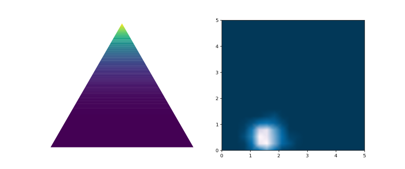
(a) Low aleatoric uncertainty, low epistemic uncertainty.

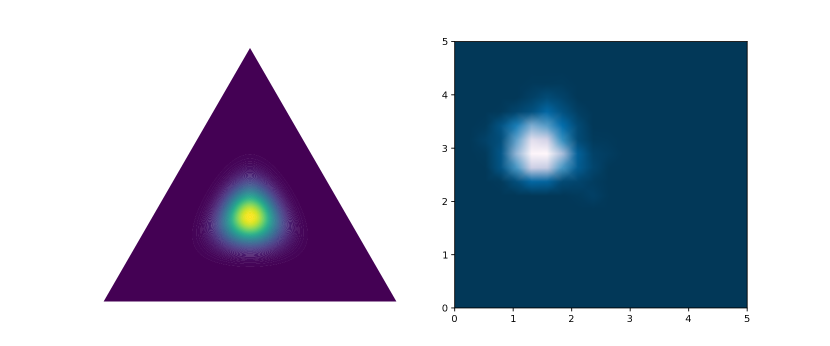
(b) High aleatoric uncertainty, low epistemic uncertainty.

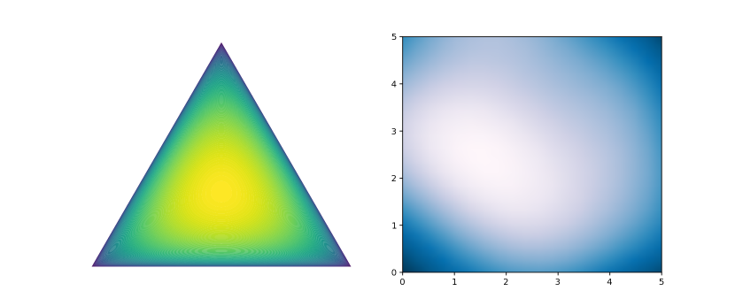
(c) High aleatoric uncertainty, high epistemic uncertainty.

Figure 1: Different behaviors of a probabilistic model under aleatoric and epistemic uncertainties for classification and regression tasks. The heat maps represent the distributions of model’s predictive distributions. The triangles represent classification simplexes and the squares represent regression parameter spaces (x-axis is the predictive mean $\mu(\bm{x}^{\ast})$ ; y-axis is the predictive variance $\sigma(\bm{x}^{\ast})$).

Deep Neural Nets (DNNs) have achieved enormous success in a wide spectrum of tasks, such as image classification (Krizhevsky et al., 2012), machine translation (Choukroun et al., 2016), and reinforcement learning (Li, 2017). Despite their remarkable predictive performance, DNNs are poor at quantifying uncertainties for their predictions. Recent studies have shown that DNNs are often overconfident in their predictions and produce mis-calibrated output probabilities for classification (Guo et al., 2017). Moreover, they can make erroneous yet wildly confident predictions for out-of-distribution samples that are very different from training data (Nguyen et al., 2015). Uncertainty quantification, a key component to equip DNNs with the ability of knowing what they do not know, has become an urgent need for many real-life applications, ranging from self-driving cars to cyber security to automatic medical diagnosis.

Existing approaches to uncertainty quantification for neural nets can be categorized into two lines. The first line is based on Bayesian neural nets (BNNs) (Denker & Lecun, 1991; MacKay, 1992). BNNs quantify predictive uncertainty by imposing probability distributions over model parameters instead of using point estimates. While BNNs provide a principled way of uncertainty quantification, exact inference of parameter posteriors is often intractable. Moreover, specifying parameter priors for BNNs is challenging because the parameters of DNNs are huge in size and uninterpretable.

Along another line, several non-Bayesian approaches have been proposed for uncertainty quantification. The most prominent idea in this line is model ensembling (Lakshminarayanan et al., 2017), which trains multiple DNNs with different initializations and uses their predictions for uncertainty estimation. However, training an ensemble of DNNs can be prohibitively expensive in practice. Other non-Bayesian methods (Geifman et al., 2019) suffer from the drawback of conflating aleatoric uncertainty—the natural randomness inherent in the task, with epistemic uncertainty—the model uncertainty caused by lack of observation data. In many tasks, it is important to separate these two sources of uncertainties. Taking active learning as an example, one would prefer to collect data from regions with high epistemic uncertainty but low aleatoric uncertainty (Hafner et al., 2018).

We propose a deep neural net model for uncertainty quantification based on neural stochastic differential equation. Our model, named SDE-Net, enjoys a number of benefits compared with existing methods: (1) It explicitly models aleatoric uncertainty and epistemic uncertainty and is able to separate the two sources of uncertainties in its predictions; (2) It is efficient and straightforward to implement, avoiding the need of specifying model prior distributions and inferring posterior distributions as in BNNs; and (3) It is applicable to both classification and regression tasks.

Our model design (Section 3) is motivated by the connection between neural nets and dynamical systems. From the dynamical system perspective, the forward passes in DNNs can be viewed as state transformations of a dynamic system, which can be defined by an NN-parameterized ordinary differential equation (ODE) (Chen et al., 2018). However, neural ODE is deterministic and cannot capture any uncertainty information. In contrast, our model characterizes the transformation of hidden states with stochastic differential equation (SDE) and adds a Brownian motion term to explicitly quantify epistemic uncertainty. Our proposed SDE-Net model thus consists of (1) a drift net that parameterizes a differential equation to fit the predictive function, and (2) a diffusion net that parameterizes the Brownian motion and encourages high diffusion for data outside the training distribution. From a control point of view, the drift net controls the system to achieve good predictive accuracy, while the diffusion net characterizes model uncertainty in a stochastic environment. We theoretically analyze the existence and uniqueness of solution to the proposed stochastic dynamical system, which provides insights to design a more efficient and stable network architecture.

Empirical results are presented in Section 4. We evaluate four tasks where uncertainty plays a fundamental role: out-of-distribution detection, misclassification detection, adversarial samples detection and active learning. We find that SDE-Net can outperform state-of-the-art uncertainty estimation methods or achieve competitive results across these tasks on various datasets.

2 Aleatoric Uncertainty and Epistemic Uncertainty

For supervised learning, we are given a training dataset $\mathcal{D}=\{\bm{x}_{j},y_{j}\}_{j=1}^{N}$; we train a model $\mathbf{M}$ parameterized by $\bm{\theta}$ and use the model $\mathbf{M}$ to make predictions for any new test instance $\bm{x}^{\ast}$. The predictive uncertainty comes from two sources (Kendall & Gal, 2017): aleatoric uncertainty and epistemic uncertainty. Aleatoric uncertainty represents the natural randomness (e.g., class overlap, data noise, unknown factors) inherent in the task and cannot be explained away with data; while epistemic uncertainty represents our ignorance about model caused by the lack of observation data and is high in regions lacking training data.

Figure 1 illustrates the behaviors of a probabilistic model under the influence of the two sources of uncertainties: (1) When both aleatoric and epistemic uncertainties are low (Figure 1(a)), the model outputs confident predictions with low variance. This makes the output distributions sharply concentrate at a simplex corner (for classification) or a small-variance region (for regression); (2) When aleatoric uncertainty is high but epistemic uncertainty is low (Figure 1(b)), the predictive distributions concentrate around the simplex center or large-variance regions; (3) When epistemic uncertainty is high (Figure 1(c)), the predictive distributions scatter in a highly diffused way over the classification simplex and the regression parameter space.

Bayesian neural networks (BNNs) model epistemic uncertainty by imposing distributions over model parameters. They are realized by first specifying prior distributions for neural net parameters, then inferring parameter posteriors and further integrating over them to make predictions. Unfortunately, such modeling of epistemic uncertainty has two drawbacks. First, it is difficult to specify the prior distributions since the parameters of DNNs are uninterpretable. Second, exact parameter posterior inference is often intractable due to the large number of parameters in DNNs. Most approaches for learning BNNs fall into one of two categories: variational inference (VI) methods (Blundell et al., 2015; Louizos & Welling, 2017; Wu et al., 2019) and Markov chain Monte Carlo (MCMC) methods (Welling & Teh, 2011; Li et al., 2016). VI methods require one to choose a family of approximating distributions, which may lead to underestimation of true uncertainties. MCMC methods are time-consuming and require maintaining many copies of the model parameters, which can be costly for large NNs. To overcome such drawbacks, we will propose a more direct and efficient way to model uncertainties.

3 Uncertainty Quantification via Neural Stochastic Differential Equation

We propose a new uncertainty aware neural net from the stochastic dynamical system perspective. The proposed method can distinguish the two sources of uncertainties with no need of specifying priors of model parameters and performing complicated Bayesian inference.

3.1 Neural Net as Deterministic Dynamical System

Our approach relies on the connection between neural nets and dynamic systems, which has been investigated in (Chen et al., 2018). As neural nets map an input $\bm{x}$ to an output $y$ through a sequence of hidden layers, the hidden representations can be viewed as the states of a dynamical system. It is thus possible to define a dynamical system by parameterizing its ordinary differential equation with a neural net. To see this, consider the transformation between layers in ResNet (He et al., 2016):

$$\bm{x}_{t+1}=\bm{x}_{t}+f(\bm{x}_{t},t),$$ (1)

where $t$ is the index of the layer while $\bm{x}_{t}$ is the hidden state at layer $t$. We rearrange this equation as $\frac{\bm{x}_{t+\Delta t}-\bm{x}_{t}}{\Delta t}=f(\bm{x}_{t},t)$ where $\Delta t=1$. Letting $\Delta t\to 0$, we obtain:

$$\lim_{\Delta\to 0}\frac{\bm{x}_{t+\Delta t}-\bm{x}_{t}}{\Delta t}=\frac{d\bm{x}_{t}}{dt}=f(\bm{x}_{t},t)\Longleftrightarrow d\bm{x}_{t}=f(\bm{x}_{t},t)dt.$$ (2)

The transformations in ResNet can thus be viewed as the discretization of a dynamical system, whose continuous dynamics is given by $f(\bm{x}_{t},t)$. The idea of the neural ODE method (Chen et al., 2018) is to parameterize $f(\bm{x}_{t},t)$ with a neural net and exploit an ODE solver to evaluate the hidden unit state wherever necessary. Such a neural ODE formulation enables evaluating hidden unit dynamics with arbitrary accuracy and enjoys better memory and parameter efficiency.

3.2 Modeling Epistemic Uncertainty with Brownian Motion

However, neural ODE is a deterministic model and cannot model epistemic uncertainty. We develop a neural SDE model to characterize a stochastic dynamical system instead of a deterministic one. The core of our neural SDE model is to capture epistemic uncertainty with Brownian motion, which is widely used to model the randomness of moving atoms or molecules in Physics (Bass, 2011).

Definition 3.1.

A standard Brownian motion $W_{t}$ is a stochastic process which satisfies the following properties: a) $W_{0}=0$; b) $W_{t}-W_{s}$ is $\mathcal{N}(0,t-s)$ for all $t\geq s\geq 0$; c) For every pair of disjoint time intervals $[t_{1},t_{2}]$ and $[t_{3},t_{4}]$, with $t_{1}<t_{2}\leq t_{3}\leq t_{4}$, the increments $W_{t_{4}}-W_{t_{3}}$ and $W_{t_{2}}-W_{t_{1}}$ are independent random variables.

We add the Brownian motion term into Eq. (2), which leads to a neural SDE dynamical system. The continuous-time dynamics of the system are then expressed as:

$$d\bm{x}_{t}=f(\bm{x}_{t},t)dt+g(\bm{x}_{t},t)dW_{t}.$$ (3)

Here, $g(\bm{x}_{t},t)$ denotes the variance of the Brownian motion and represents the epistemic uncertainty for the dynamical system. This variance is determined by which region the system is in. As shown in Fig. 2, if the system is in the region with abundant training data and low epistemic uncertainty, the variance of the Brownian motion will be small; if the system is in the region with scarce training data and high epistemic uncertainty, the variance of the Brownian motion will be large. We can thus obtain an epistemic uncertainty estimate from the variance of the final time solution $x_{T}$.

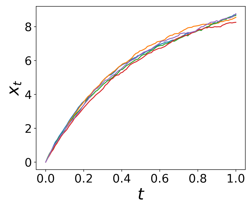
(a) System in the region with low uncertainty

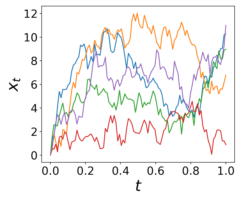
(b) System in the region with high uncertainty

Figure 2: 1-D trajectories of a linear SDE for five simulations. When the system is in the region with low uncertainty, i.e. small $g(\bm{x}_{t},t)$, the trajectories are more deterministic with small variance. When the system is in the region with high uncertainty, i.e. large $g(\bm{x}_{t},t)$, the trajectories are more scattered with large variance.

3.3 SDE-Net for Uncertainty Estimation

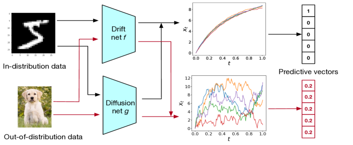
Figure 3: Components of the proposed SDE-Net. For in-distribution data, the system is dominated by the drift net $f$ and achieves good predictive accuracy; for out-of-distribution data, the system is dominated by the diffusion net $g$ and shows high diffusion.

As discussed above, we can quantify epistemic uncertainty using Brownian motion. To make the system able to achieve good predictive accuracy and meanwhile provide reliable uncertainty estimates, we design our SDE-Net model to use two separate neural nets to represent the drift and the diffusion of the system as in Fig. 3.

The drift net $f$ in SDE-Net aims to control the system to achieve good predictive accuracy. Another important role of the drift net $f$ is to capture aleatoric uncertainty. This is achieved by representing model output as a probabilistic distribution, e.g., categorical distribution for classification and Gaussian distribution for regression.

The diffusion net $g$ in SDE-Net represents the diffusion of the system. The diffusion of the system should satisfy the following: (1) For regions in the training distribution, the variance of the Brownian motion should be small (low diffusion). The system state is dominated by the drift term in this area and the output variance should be small; (2) For regions outside the training distribution, the variance of the Brownian motion should be large and the system is chaotic (high diffusion). In this case, the variance of the outputs for multiple evaluations should be large.

Based on the above desired properties, we propose the following objective function for training our SDE-Net model:

$$\min_{\bm{\theta}_{f}}{\rm E}_{\bm{x}_{0}\sim P_{\text{train}}}{\rm E}(L(\bm{x}_{T}))+\min_{\bm{\theta}_{g}}{\rm E}_{\bm{x}_{0}\sim P_{\text{train}}}g(\bm{x}_{0};\bm{\theta}_{g})$$

$$+\max_{\bm{\theta}_{g}}{\rm E}_{\tilde{\bm{x}}_{0}\sim P_{\text{OOD}}}g(\tilde{\bm{x}}_{0};\bm{\theta}_{g})$$

$$s.t.\quad d\bm{x}_{t}=\underbrace{f(\bm{x}_{t},t;\bm{\theta}_{f})}_{\text{drift neural net}}dt+\underbrace{g(\bm{x}_{0};\bm{\theta}_{g})}_{\text{diffusion neural net}}dW_{t},$$ (4)

where $L(\cdot)$ is the loss function dependent on the task, e.g. cross entropy loss for classification, $T$ is the terminal time of the stochastic process, $P_{\text{train}}$ is the distribution for training data, and $P_{\text{OOD}}$ is the out-of-distribution (OOD) data. To obtain OOD data, we choose to add additive Gaussian noise to obtain noisy inputs $\tilde{\bm{x}}_{0}=\bm{x}_{0}+\bm{\epsilon}$ and then distribute the inputs according to the convolved distribution as in (Hafner et al., 2018). An alternative is to use a different, real dataset as a set of samples from the OOD. However, this requires a careful choice of a real dataset to avoid overfitting (Lee et al., 2018).

Unlike the traditional neural nets where each layer has its own parameters, the parameters in our proposed SDE-Net are shared by each layer. This can decrease the number of parameters and leads to significant memory reduction. In the objective function, we also make a simplification that the variance of the diffusion term is only determined by the starting point $\bm{x}_{0}$ instead of the instantaneous value $\bm{x}_{t}$, which is usually sufficient and can make the optimization procedure easier.

Uncertainty Quantification: Once an SDE-Net is learned, we can obtain multiple random realizations of the SDE-Net to get samples $\{\bm{x}_{T}\}_{m=1}^{M}$ and then compute the two uncertainties from them. The aleatoric uncertainty is given by the expected predictive entropy $\mathbb{E}_{p(\bm{x}_{T}|\bm{x}_{0},\bm{\theta}_{f,g})}[\mathcal{H}[p(y|\bm{x}_{T})]]$ in classification and expected predictive variance $\mathbb{E}_{p(\bm{x}_{T}|\bm{x}_{0},\bm{\theta}_{f,g})}[\sigma(\bm{x}_{T})]$ in regression. The epistemic uncertainty is given by the variance of the final solution ${\rm Var}(\bm{x}_{T})$. This sampling-and-computing operation shares similar spirit with the traditional ensembling method. However, a key difference exists between the two: ensembling methods require training multiple deterministic NNs, while our method just trains one neural SDE model and uses the Brownian motion to encode uncertainty, which incurs much lower time and memory costs.

3.4 Theoretical Analysis

In this subsection, we study the existence and uniqueness of the solution $\bm{x}_{t}(0\leq t\leq T)$ of the proposed stochastic system. Through this theoretical analysis, we can gain insights in designing a more effective network architecture for both the drift net $f$ and the diffusion net $g$.

Theorem 1.

When there exists $C>0$ such that

$$\begin{split}&||f(\bm{x},t;\bm{\theta}_{f})-f(\bm{y},t;\bm{\theta}_{f})||+||g(\bm{x};\bm{\theta}_{g})-g(\bm{y};\bm{\theta}_{g})||\\ &\leq C||\bm{x}-\bm{y}||,\quad\forall\bm{x},\bm{y}\in\mathcal{R}^{n},t\geq 0.\end{split}$$ (5)

Then, for every $\bm{x}_{0}\in\mathcal{R}^{n}$, there exists a unique continuous and adapted process $(\bm{x}_{t}^{x_{0}})_{t\geq 0}$ such that for $t\geq 0$

$$\bm{x}_{t}^{\bm{x}_{0}}=\bm{x}_{0}+\int_{0}^{t}f(\bm{x}_{s}^{\bm{x}_{0}},t;\bm{\theta}_{f})ds+\int_{0}^{t}g(\bm{x}_{0};\bm{\theta}_{g})dW_{s}$$ (6)

Moreover, for every $T\geq 0$, $\textup{E}(\textup{sup}_{1\leq s\leq T}|\bm{x}_{s}|^{2})<+\infty.$

The proof of Theorem 1 can be found in the supplementary material.

Remark. According to Theorem 1, $f(\bm{x},t;\bm{\theta}_{f})$ and $g(\bm{x};\bm{\theta}_{g})$ must both be uniformly Lipschitz continuous. This can be satisfied by using Lipshitz nonlinear activations in the network architectures, such as ReLU, sigmoid and Tanh (Anil et al., 2019). However, if we naïvely optimize the loss function in Equation (4), $g(\bm{x}_{0};\bm{\theta}_{g})$ can be infinitely large for the input from out-of-distribution. This will lead to explosive solution and make the optimization procedure unstable. To solve this problem, we define the maximum value of the output of $g(\bm{x};\bm{\theta}_{g})$ as a hyper-parameter $\sigma_{\rm max}$. Then, the output of the diffusion neural net is given by a sigmoid function times $\sigma_{\rm max}$.

3.5 SDE-Net Training

There is no closed form solution to the true final random variable $\bm{x}_{T}$. In principle, we can simulate the stochastic dynamics using any high-order numerical solver with adaptive step size (Platen, 1999). However, high-order numerical methods can be costly in the context of deep learning where the input can have thousands of dimensions. Since we focus on supervised learning and uncertainty quantification, we choose to use the simple Euler-Maruyama scheme with fixed step size (Kloeden & Platen, 1992) for efficient network training. Under such a scheme, the time interval $[0,T]$ is divided into $N$ subintervals. Then, we can simulate the SDE by:

$$\bm{x}_{k+1}=\bm{x}_{k}+f(\bm{x}_{k},t;\bm{\theta}_{f})\Delta t+g(\bm{x}_{0};\bm{\theta}_{g})\sqrt{\Delta t}Z_{k}$$ (7)

where $Z_{k}\sim\mathcal{N}(0,1)$ is the standard Gaussian random variable and $\Delta t=T/N$. We will show that empirically it suffices to sample only one path for each data point during training time. The number of steps for solving the SDE can be considered equivalently as the number of layers in the definition of traditional neural nets. Then, the training of SDE-Net is actually the forward and backward propagations as in standard neural nets, which can be easily implemented with libraries such as Tensorflow and Pytorch. The drift neural net $f$ and the diffusion neural net $g$ are optimized alternately, as shown in Algorithm 1.

Algorithm 1 Training of SDE-Net. $h_{1}$ is the downsampling layer; $h_{2}$ is the fully connected layer; $f$ and $g$ are the drift net and diffusion net; $L$ is the loss function.

  Initialize $h_{1},f,g$ and $h_{2}$

  for $\#$ training iterations do

     Sample minibatch of $N_{M}$ data from in-distribution: $\mathbf{X}^{N_{M}}\sim p_{\text{train}}(x)$

     Forward through the downsampling layer: $\mathbf{X}_{0}^{N_{M}}=h_{1}(\mathbf{X}^{N_{M}})$

     Forward through the SDE-Net block:

     for $k=0$ to $N-1$ do

        Sample $\mathbf{Z}_{k}^{N_{M}}\sim\mathcal{N}(0,\mathbf{I})$

        $\mathbf{X}_{k+1}^{N_{M}}=\mathbf{X}_{k}^{N_{M}}+f(\mathbf{X}_{k}^{N_{M}},t)\Delta t+g(\mathbf{X}_{0}^{N_{M}})\sqrt{\Delta t}\mathbf{Z}_{k}$

     end for

     Forward through the fully connected layer: $\mathbf{X}_{\text{f}}^{N_{M}}=h_{2}(\mathbf{X}_{k}^{N_{M}})$

     Update $h_{1},h_{2}$ and $f$ by $\nabla_{h_{1},h_{2},f}\frac{1}{N_{M}}L(\mathbf{X}_{\text{f}}^{N_{M}})$

     Sample minibatch of $N_{M}$ data from out-of-distribution: $\mathbf{X}^{N_{M}}\sim p_{\text{OOD}}(x)$

     Forward through the downsampling layer: $\mathbf{X}_{0}^{N_{M}},\tilde{\mathbf{X}}_{0}^{N_{M}}=h_{1}(\mathbf{X}^{N_{M}}),h_{1}(\tilde{\mathbf{X}}^{N_{M}})$

     Update $g$ by $\nabla_{g}g(\mathbf{X}_{0}^{N_{M}})-\nabla_{g}g(\tilde{\mathbf{X}_{0}}^{N_{M}})$

  end for

4 Experiments

In this section, we study how the estimated uncertainty can improve model robustness and label efficiency. We first study three tasks on model robustness: (1) out-of-distribution detection, (2) misclassification detection, and (3) adversarial sample detection. We then study how the estimated uncertainties can improve label efficiency on active learning.

4.1 Experimental Setup

We compare our SDE-Net model with the following methods: (1) Threshold (Hendrycks & Gimpel, 2017), which is used in the deterministic DNNs (2) MC-dropout (Gal & Ghahramani, 2016), (3) DeepEnsemble(Lakshminarayanan et al., 2017), (4) Prior network (PN) (Malinin & Gales, 2018), (5) Bayes by Backpropagation (BBP) (Blundell et al., 2015), (6) preconditioned Stochastic gradient Langevin dynamics (p-SGLD) (Li et al., 2016).

The network architecture of the compared methods is a residual net (Chen et al., 2018). For our method, we use one SDE-Net block in place of residual blocks and set the number of subintervals as the number of residual blocks in ResNet for fair comparison—the number of hidden layers in SDE-Net is the same as the baseline models under such settings. For our SDE-Net, we sample one path during training and perform 10 stochastic forward passes at test time in all experiments.

As PN and SDE-Net both involve OOD samples during the training process, we purturb the training data with Gaussian noise (zero mean and variance four for both MNIST and SVHN) as pseudo OOD data. Our supplementary materials provide more details about the implementation, setup, and additional experimental results.

Table 1: Classification and out-of-distribution detection results on MNIST and SVHN. All values are in percentage, and larger values indicates better detection performance. We report the average performance and standard deviation for 5 random initializations.

ID	OOD	Model	# Parameters	Classification accuracy	TNR at TPR $95\%$	AUROC	Detection accuracy	AUPR in	AUPR out
MNIST	SEMEION	Threshold	0.58M	$99.5\pm 0.0$	$94.0\pm 1.4$	$98.3\pm 0.3$	$94.8\pm 0.7$	$99.7\pm 0.1$	$89.4\pm 1.1$
		DeepEnsemble	0.58M $\times$ 5	$\bm{99.6}\pm$ NA	$96.0\pm$ NA	$98.8\pm$ NA	$95.8\pm$ NA	$99.8\pm$ NA	$91.3\pm$ NA
		MC-dropout	0.58M	$99.5\pm 0.0$	$92.9\pm 1.6$	$97.6\pm 0.5$	$94.2\pm 0.7$	$99.6\pm 0.1$	$88.5\pm 1.7$
		PN	0.58M	$99.3\pm 0.1$	$93.4\pm 2.2$	$96.1\pm 1.2$	$94.5\pm 1.1$	$98.4\pm 0.7$	$88.5\pm 1.3$
		BBP	1.02M	$99.2\pm 0.3$	$75.0\pm 3.4$	$94.8\pm 1.2$	$90.4\pm 2.2$	$99.2\pm 0.3$	$76.0\pm 4.2$
		p-SGLD	0.58M	$99.3\pm 0.2$	$85.3\pm 2.3$	$89.1\pm 1.6$	$90.5\pm 1.3$	$93.6\pm 1.0$	$82.8\pm 2.2$
		SDE-Net	0.28M	$99.4\pm 0.1$	$\bm{99.6}\pm 0.2$	$\bm{99.9}\pm 0.1$	$\bm{98.6}\pm 0.5$	$\bm{100.0}\pm 0$	$\bm{99.5}\pm 0.3$
MNIST	SVHN	Threshold	0.58M	$99.5\pm 0.0$	$90.1\pm 2.3$	$96.8\pm 0.9$	$92.9\pm 1.1$	$90.0\pm 3.5$	$98.7\pm 0.3$
		DeepEnsemble	0.58M$\times 5$	$\bm{99.6}\pm$ NA	$92.7\pm$ NA	$98.0\pm$ NA	$94.1\pm$ NA	$94.5\pm$ NA	$99.1\pm$ NA
		MC-dropout	0.58M	$99.5\pm 0.0$	$88.7\pm 0.6$	$95.9\pm 0.4$	$92.0\pm 0.3$	$87.6\pm 2.0$	$98.4\pm 0.1$
		PN	0.58 M	$99.3\pm 0.1$	$90.4\pm 2.8$	$94.1\pm 2.2$	$93.0\pm 1.4$	$73.2\pm 7.3$	$98.0\pm 0.6$
		BBP	1.02M	$99.2\pm 0.3$	$80.5\pm 3.2$	$96.0\pm 1.1$	$91.9\pm 0.9$	$92.6\pm 2.4$	$98.3\pm 0.4$
		p-SGLD	0.58M	$99.3\pm 0.2$	$94.5\pm 2.1$	$95.7\pm 1.3$	$95.0\pm 1.2$	$75.6\pm 5.2$	$98.7\pm 0.2$
		SDE-Net	0.28M	$99.4\pm 0.1$	$\bm{97.8}\pm 1.1$	$\bm{99.5}\pm 0.2$	$\bm{97.0}\pm 0.2$	$\bm{98.6}\pm 0.6$	$\bm{99.8}\pm 0.1$
SVHN	CIFAR10	Threshold	0.58M	$95.2\pm 0.1$	$66.1\pm 1.9$	$94.4\pm 0.4$	$89.8\pm 0.5$	$96.7\pm 0.2$	$84.6\pm 0.8$
		DeepEnsemble	0.58M$\times$5	$\bm{95.4}\pm$ NA	$66.5\pm$ NA	$94.6\pm$ NA	$90.1\pm$ NA	$97.8\pm$ NA	$84.8\pm$ NA
		MC-dropout	0.58M	$95.2\pm 0.1$	$66.9\pm 0.6$	$94.3\pm 0.1$	$89.8\pm 0.2$	$97.6\pm 0.1$	$84.8\pm 0.2$
		PN	0.58M	$95.0\pm 0.1$	$66.9\pm 2.0$	$89.9\pm 0.6$	$87.4\pm 0.6$	$92.5\pm 0.6$	$82.3\pm 0.9$
		BBP	1.02M	$93.3\pm 0.6$	$42.2\pm 1.2$	$90.4\pm 0.3$	$83.9\pm 0.4$	$96.4\pm 0.2$	$73.9\pm 0.5$
		p-SGLD	0.58M	$94.1\pm 0.5$	$63.5\pm 0.9$	$94.3\pm 0.4$	$87.8\pm 1.2$	$97.9\pm 0.2$	$83.9\pm 0.7$
		SDE-Net	0.32 M	$94.2\pm 0.2$	$\bm{87.5}\pm 2.8$	$\bm{97.8}\pm 0.4$	$\bm{92.7}\pm 0.7$	$\bm{99.2}\pm 0.2$	$\bm{93.7}\pm 0.9$
SVHN	CIFAR100	Threshold	0.58M	$95.2\pm 0.1$	$64.6\pm 1.9$	$93.8\pm 0.4$	$88.3\pm 0.4$	$97.0\pm 0.2$	$83.7\pm 0.8$
		DeepEnsemble	0.58M $\times 5$	$\bm{95.4}\pm$ NA	$64.4\pm$ NA	$93.9\pm$ NA	$89.4\pm$ NA	$97.4\pm$ NA	$84.8\pm$ NA
		MC-dropout	0.58M	$95.2\pm 0.1$	$65.5\pm 1.1$	$93.7\pm 0.2$	$89.3\pm 0.3$	$97.1\pm 0.2$	$83.9\pm 0.4$
		PN	0.58M	$95.0\pm 0.1$	$65.8\pm 1.7$	$89.1\pm 0.8$	$86.6\pm 0.7$	$91.8\pm 0.8$	$81.6\pm 1.1$
		BBP	1.02M	$93.3\pm 0.6$	$42.4\pm 0.3$	$90.6\pm 0.2$	$84.3\pm 0.3$	$96.5\pm 0.1$	$75.2\pm 0.9$
		p-SGLD	0.58M	$94.1\pm 0.5$	$62.0\pm 0.5$	$91.3\pm 1.2$	$86.0\pm 0.2$	$93.1\pm 0.8$	$81.9\pm 1.3$
		SDE-Net	0.32M	$94.2\pm 0.2$	$\bm{83.4}\pm 3.6$	$\bm{97.0}\pm 0.4$	$\bm{91.6}\pm 0.7$	$\bm{98.8}\pm 0.1$	$\bm{92.3}\pm 1.1$

4.2 Out-of-Distribution Detection

Our first task is out-of-distribution (OOD) detection, which aims to use uncertainty to help the model recognize out-of-distribution samples at test time. In open-world settings, the model needs to deal with continuous data that may come from different data distributions or unseen classes. For OOD samples, it is wiser to let the model say ‘I don’t know’ instead of making an absurdly wrong predictions. We investigate the OOD detection task under both classification and regression settings. Following previous work (Hendrycks & Gimpel, 2017), we use four metrics for the OOD detection task: (1) True negative rate (TNR) at $95\%$ true positive rate (TPR); (2) Area under the receiver operating characteristic curve (AUROC); (3) Area under the precision-recall curve (AUPR); and (4) Detection accuracy. Larger values of them indicate better detection performance.

OOD detection for classification. We first evaluate the performance of different models for OOD detection in classification tasks. For fair comparison, all the methods use the probability of the final predicted class for detection. Table 1 shows the OOD detection performance as well as the classification accuracy on two image classification datasets: MNIST and SVHN. We mix different test OOD datasets with the target dataset (MNIST or SVHN) and evaluate the performance of different models in OOD detection. As shown, SDE-Net consistently achieves the best OOD detection performance among all the models under different combinations. DeepEnsemble is the strongest among the baselines but it still underperforms SDE-Net consistently. Furthermore, DeepEnsemble needs to train multiple DNNs and incurs much larger computational costs. While PN and SDE-Net both use pseudo OOD data (with Gaussian noise) during training, SDE-Net consistently outperforms PN in all the settings. In addition to using the Gaussian-purturbed OOD data, we also compared the performance of SDE-Net and PN when using real-life OOD datasets during training (see supplementary material). We find that PN is easy to be overfitted, while our SDE-Net is more robust to the choice of OOD data used for training.

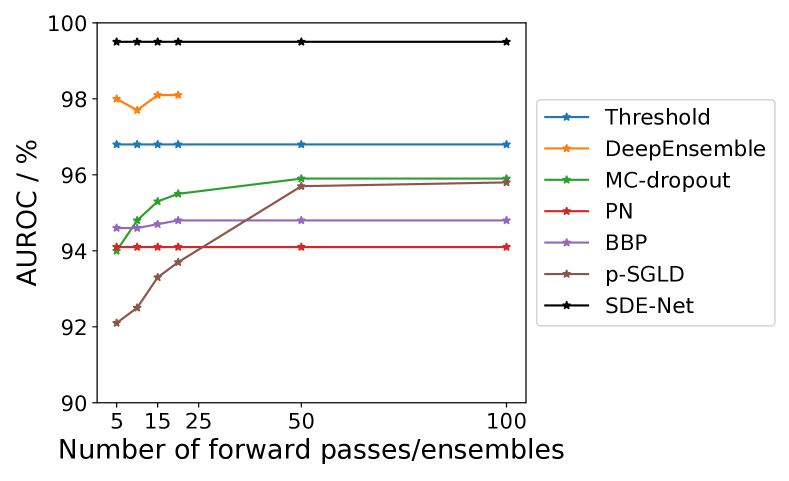
Figure 4: Effect of number of forward passes / ensembles on out-of-distribution (OOD) detection. We use MNIST as the ID data and SVHN as the OOD data.

Fig. 4 shows the impact of the number of forward passes or ensembles on OOD detection, using MNIST as the ID data and SVHN as the OOD data. As we can see, the BNNs (MC-dropout, p-SGLD and BBP) require more samples than SDE-Net to reach their peak performance at test time. For DeepEnsemble, its performance is already almost saturated when using five nets and larger ensemble sizes can bring little performance gain.

In addition to the OOD detection metrics, we also studied the classification accuracy of different models. We find that the predictive performance of SDE-Net is very close to state-of-the-art results even with significantly fewer parameters. One can further achieve better results by stacking multiple SDE-Net blocks together.

OOD detection for regression. We now investigate OOD detection in regression tasks. Different from classification, few works have studied the OOD detection task for regression. We use the Year Prediction MSD dataset (Dua & Graff, 2017) as training data and the Boston Housing dataset (Bos, ) as test OOD data. Threshold and PN are excluded here since they only apply to classification tasks. To detect OOD samples for regression tasks, all the methods rely on the variance of the predictive mean. Table 6 shows the OOD detection performance for different methods. The results of other metrics are put into the supplementary material due to the space limit. Because of the imbalance of the test ID and OOD data, AUPR out is a better metric than AUPR in. OOD detection for regression is more difficult than for classification, because regression is a continuous and unbounded problem which makes uncertainty estimation difficult. For this challenging task, all the baselines perform quite poorly, yet SDE-Net still achieves strong performance. The reason is that the diffusion net in SDE-Net directly models the relationship between the input data and epistemic uncertainty, which encourages SDE-Net to output large uncertainty for OOD data and low uncertainty for ID data even for this challenging task.

Table 2: Out-of-distribution detection for regression on Year Prediction MSD + Boston Housing. We report the average performance and standard deviation for 5 random initializations.

Model	# Parameters	RMSE	AUROC	AUPR out
DeepEnsemble	14.9K$\times 5$	$\bm{8.6}\pm$ NA	$59.8\pm$ NA	$1.3\pm$ NA
MC-dropout	14.9K	$8.7\pm 0.0$	$53.0\pm 1.2$	$1.1\pm 0.1$
BBP	30.0K	$9.5\pm 0.2$	$56.8\pm 0.9$	$1.3\pm 0.1$
p-SGLD	14.9K	$9.3\pm 0.1$	$52.3\pm 0.7$	$1.1\pm 0.2$
SDE-Net	12.4K	$8.7\pm 0.1$	$\bm{84.4}\pm 1.0$	$\bm{21.3}\pm 4.1$

4.3 Misclassification Detection

Besides OOD data detection, another important use of uncertainty is to make the model aware when it may make mistakes at test time. Thus, our second task is misclassification detection (Hendrycks & Gimpel, 2017), which aims at leveraging the predictive uncertainty to identify test samples on which the model have misclassified. Table 7 shows the misclassification detection results for different models on MNIST and SVHN. p-SGLD achieves the best overall performance for this task. SDE-Net achieves comparable performance with DeepEnsemble and outperforms other baselines. However, p-SGLD needs to store the copies of the parameters for evaluation, which can be prohibitively costly for large NNs. DeepEnsemble requires training multiple models and incurs high computational cost. Therefore, we argue that SDE-Net is a better choice for the misclassification task in practice.

Table 3: Misclassification detection performance on MNIST and SVHN. We report the average performance and standard deviation for 5 random initializations.

Data	Model	AUROC	AUPR succ	AUPR err
MNIST	Threshold	$94.3\pm 0.9$	$99.8\pm 0.1$	$31.9\pm 8.3$
	DeepEnsemble	$\bm{97.5}\pm$ NA	$\bm{100.0}\pm$ NA	$41.4\pm$ NA
	MC-dropout	$95.8\pm 1.3$	$99.9\pm 0.0$	$33.0\pm 6.7$
	PN	$91.8\pm 0.7$	$99.8\pm 0.0$	$33.4\pm 4.6$
	BBP	$96.5\pm 2.1$	$\bm{100.0}\pm 0.0$	$35.4\pm 3.2$
	P-SGLD	$96.4\pm 1.7$	$\bm{100.0\pm}0.0$	$\bm{42.0\pm}2.4$
	SDE-Net	$96.8\pm 0.9$	$\bm{100.0\pm}0.0$	$36.6\pm 4.6$
SVHN	Threshold	$90.1\pm 0.3$	$99.3\pm 0.0$	$42.8\pm 0.6$
	DeepEnsemble	$91.0\pm$ NA	$\bm{99.4}\pm$ NA	$46.5\pm$ NA
	MC-dropout	$90.4\pm 0.6$	$99.3\pm 0.0$	$45.0\pm 1.2$
	PN	$84.0\pm 0.4$	$98.2\pm 0.2$	$43.9\pm 1.1$
	BBP	$91.8\pm 0.2$	$99.1\pm 0.1$	$50.7\pm 0.9$
	P-SGLD	$\bm{93.0}\pm 0.4$	$\bm{99.4}\pm 0.1$	$48.6\pm 1.8$
	SDE-Net	$92.3\pm 0.5$	$\bm{99.4\pm}0.0$	$\bm{53.9}\pm 2.5$

4.4 Adversarial Sample Detection

Our third task studies adversarial sample detection. Existing works (Szegedy et al., 2014; Goodfellow et al., 2015b) have shown that DNNs are extremely vulnerable to adversarial examples crafted by adding small adversarial perturbations. The ability to detect such adversarial samples is important for AI safety. Different from existing literature on adversarial training, we do not use adversarial training but only examine the uncertainty-aware models’ ability in detecting adversarial samples. We study two attacks: Fast Gradient-Sign Method (FGSM) (Goodfellow et al., 2015a), and Projected Gradient Descent (PGD) (Madry et al., 2018).

Fig. 5 shows the detection performance of different models when facing FGSM attacks. As shown, when the perturbation size $\epsilon$ varies, SDE-Net can achieve similar AUROC with p-SGLD and outperforms all other methods. On the simpler MNIST dataset, all methods can achieve $\sim$100% AUROC when the perturbation size is large. However, on the more challenging SVHN dataset, only SDE-Net still converges to 100% AUROC, while other baselines achieve only about 90% AUROC even with perturbation size of one.

Fig. 6 shows the detection performance of different models when facing PGD attacks. We use the default parameters in (Madry et al., 2018) and plot the AUROC curve versus the number of PGD iterations. Under the stronger PGD attacks, the AUROCs of all the baselines on MNIST drop below 70% after 60 iterations, while SDE-Net can still achieves over 80% AUROC after 100 iterations. On SVHN, we observe a different picture where all the methods quickly become overconfident except for the costly DeepEnsemble method. This is likely due to higher dimensionality of the data manifold in SVHN. Further work is needed to design efficient and robust uncertainty-aware models that can detect high-dimensional adversarial samples generated by such strong attackers.

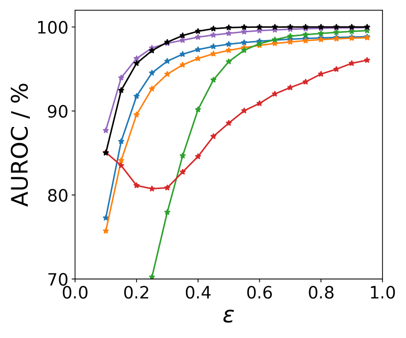
(a) MNIST

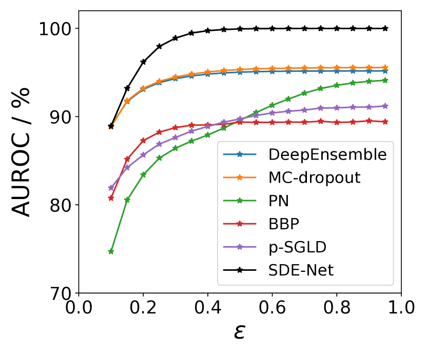
(b) SVHN

Figure 5: The performance of adversarial sample detection under FGSM attacks. $\epsilon$ is the step size in FGSM.

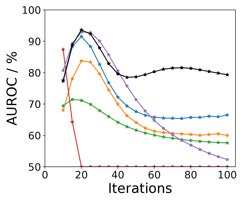
(a) MNIST

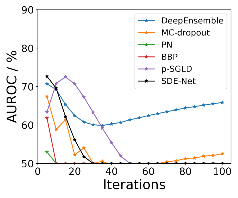
(b) SVHN

Figure 6: The performance of adversarial sample detection under PGD attacks.

4.5 Active Learning

Finally, we study how the estimated uncertainties can improve label efficiency for active learning. Uncertainty plays an important role in active learning. Intuitively, accurate uncertainty estimates can dramatically reduce the amount of labeled data for model training, while inaccurate estimates make the model choose uninformative instances and even lead to worse performance due to overfitting. For active learning, we use the acquisition function proposed in (Hafner et al., 2018):

$$\{\bm{x}_{\rm new},y_{\rm new}\}\sim p_{\rm new}(\bm{x},y)\propto\left(1+\frac{{\rm Var}[\mu(\bm{x})]}{\sigma^{2}(\bm{x})}\right)^{2}.$$ (8)

This acquisition function allows us to extract the data from the region where the model has high epistemic uncertainty but the data has low aleatoric noise. For the deterministic neural network, we use the predictive variance as a proxy since it cannot model epistemic uncertainty.

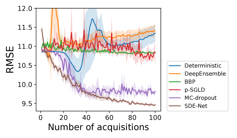
Figure 7: The performance of different models for active learning on the Year Prediction MSD dataset. We report the average performance and standard deviation for 5 random initializations.

We use the Year Prediction MSD regression dataset, where the task is to predict the release year of a song from 90 audio features. It has total 515,345 data points of which 463,715 are for training. We experiment with the following procedure. Starting from 50 labels, the models select a batch of 50 additional labels in every 100 epochs. The remaining data points in the training dataset are available for acquisition, and we evaluate performance on the whole test set.

As we can see from Fig. 7, the RMSE of SDE-Net consistently decreases as we acquire more labeled data. Such results show that SDE-Net successfully acquire data from informative region. However, the performance gain of BBP and p-SGLD are still negligible even after 100 acquisitions. We can also observe that the performance of the deterministic NN and DeepEnsemble start to degrade after several iterations. This is because they keep extracting uninformative data points and thus suffer from overfitting due to the small training data size.

5 Additional Related Work

Uncertainty estimation: BNNs is a principled way for uncertainty quantification. Performing exact Bayesian inference is inefficient and computationally intractable. A common workaround is to use approximation methods like variational inference (Blundell et al., 2015; Louizos & Welling, 2017; Shi et al., 2018; Louizos & Welling, 2016; Zhang et al., 2018), Laplace approximation (Ritter et al., 2018), expectation propagation (Li et al., 2015), stochastic gradient MCMC (Li et al., 2016; Welling & Teh, 2011) and so on. Gal & Ghahramani (2016, 2015) proposed to use Monte-Carlo Dropout (MC-dropout) at test time to estimate the uncertainty which has a nice interpretation in terms of variational Bayes. Another key element which can affect the performance of BNNs is the choice of prior distribution. The most common prior to use is the independent Gaussian distribution which can only give limited and even biased information for uncertainty. Recently, Hafner et al. (2018) proposed to use noise contrastive priors (NCPs) to obtain reliable uncertainty estimates. Functional variational BNNs (fBNNs) (Sun et al., ) employ Gaussian Process (GP) priors and use BNNs for inference.

A number of non-Bayesian methods have also been proposed for uncertainty quantification. DeepEnsemble (Lakshminarayanan et al., 2017) trains an ensemble of NNs and reports competitive uncertainty estimates to MC dropout. Pereyra et al. (2017) adds an entropy penalty as the network regularizer. In (Lee et al., 2018), the authors proposed to minimize a new confidence loss to both a sharp predictive distribution for training data and a flat predictive distribution for OOD data. The OOD data is generated by using a generative model. Prior network (Malinin & Gales, 2018, 2019) parametrized a Dirichlet distribution over categorical output distributions which allows high uncertainty for OOD data, but it is only applicable to classification tasks.

Neural dynamic system: E (2017) first observed the link between ResNet and ODE (Ince, 1956). The residual block which is formulated as $x_{n+1}=x_{n}+f(x_{n})$ can be considered as the forward Euler discretization of the ODE $dx_{t}=f(x_{t})$. In (Lu et al., 2018), the authors show that many state-of-the-art deep network architectures, such as PolyNet (Zhang et al., 2017), FractalNet (Larsson et al., 2017) and RevNet (Gomez et al., 2017), can be regarded as different discretization schemes of ODEs. Chen et al. (2018) further generalized the discrete ResNet to a continuous-depth network by making use of the existing ODE solvers. The adjoint method (Plessix, 2006) is used during ODE-Net training, which allows constant memory cost and adaptive computation. However, these works all focus on improving the predictive accuracy while our work quantifies model uncertainty based on the SDE formulation and the introduced Brownian motion term. Concurrently with this paper, Tzen & Raginsky (2019) establish a connection between infinitely deep residual networks and solutions to SDE. Li et al. (2020) propose a generalization of the adjoint method to compute gradients through solutions of SDEs and apply a latent SDE for continuous time-series data modeling. Our approaches were developed simultaneously but focus on using neural SDEs for uncertainty quantification.

6 Conclusion

We proposed a neural stochastic differential equation model (SDE-Net) for quantifying uncertainties in deep neural nets. The proposed model can separate different sources of uncertainties compared with existing non-Bayesian methods while being much simpler and more straightforward than Bayesian neural nets. Through comprehensive experiments, we demonstrated that SDE-Net has strong performance compared to state-of-the-art techniques for uncertainty quantification on both classification and regression tasks. To the best of our knowledge, our work represents the first study which establishes the connection between stochastic dynamical system and neural nets for uncertainty quantification. As the approach is general and efficient, we believe this is a promising direction for equipping neural nets with meaningful uncertainties in many safety-critical applications.

S. 1 Proof of Theorem 1

Theorem 1 can be seen as a special case of the existence and uniqueness theorem of a general stochastic differential equation. The following derivation is adapted from (Lalley, 2016). To prove Theorem 1, we first introduce two lemmas.

Lemma 1.

Let $y(t)$ be a nonnegative function that satisfies the following condition: for some $T\leq\infty$, there exist constants $A,B\geq 0$ such that:

$$y(t)\leq A+B\int_{0}^{t}y(s)ds<\infty\quad\text{for all}\quad 0\leq t\leq T.$$ (9)

Then

$$y(t)\leq Ae^{Bt}\quad\text{for all}\quad 0\leq t\leq T.$$ (10)

Proof.

W.l.o.g., we assume that $C=\int_{0}^{T}y(s)ds<\infty$ and that $T<\infty$. Then, we can obtain that $y(t)$ is bounded by $D\equiv A+BC$ in the interval $[0,T]$. By iterating over inequality (9), we have:

$$\begin{split}y(t)&\leq A+B\int_{0}^{t}y(s)ds\\ &\leq A+B\int_{0}^{t}(A+B)\int_{0}^{s}y(r)drds\\ &\leq A+BAt+B^{2}\int_{0}^{t}\int_{0}^{s}(A+B\int_{0}^{r}y(q)dq)drds\\ &\leq A+BAt+B^{2}At^{2}/2!+B^{3}\int_{0}^{t}\int_{0}^{s}\int_{0}^{r}(A+B\int_{0}^{q}y(p)dp)dqdrds\\ &\leq\cdots.\end{split}$$ (11)

After $k$ iterations, the first $k$ terms are the series for $Ae^{Bt}$. The last term is a $(k+1)$-fold iterated integral $I_{k}$. Because $y(t)\leq D$ in the interval $[0,T]$, the integral $I_{k}$ is bounded by $B^{k}Dt^{k+1}/(k+1)!$. This converges to zero uniformly for $t\leq T$ as $k\rightarrow\infty$. Hence, inequality (10) follows. ∎

Lemma 2.

Let $y_{n}(t)$ be a sequence of nonnegative functions such that for some constants $B,C<\infty$,

$$\begin{split}&\quad y_{0}(t)\leq C\quad\text{for all}\quad t\leq T\quad\text{and}\\ &y_{n+1}(t)\leq B\int_{0}^{t}y_{n}(s)ds<\infty\quad\text{for all}\quad t\leq T\quad\text{and}\quad n=0,1,2,\cdots.\end{split}$$ (12)

Then,

$$y_{n}(t)\leq CB^{n}t^{n}/n!\quad\text{for all}\quad t\leq T.$$ (13)

Proof.

$$\begin{split}y_{1}(t)&\leq B\int_{0}^{t}Cds=BCt\\ y_{2}(t)&\leq B\int_{0}^{t}BCsds=CB^{2}t^{2}/2!\\ y_{3}(t)&\leq B\int_{0}^{t}CB^{2}s^{2}/2ds=CB^{3}t^{3}/3!\\ \cdots.\end{split}$$ (14)

After $n$ iterations, we have $y_{n}(t)\leq CB^{n}t^{n}/n!$ for all $t\leq T$. ∎

Suppose that for some initial value $\bm{x}_{0}$ there are two different solutions:

$$\begin{split}&\bm{x}_{t}=\bm{x}_{0}+\int_{0}^{t}f(\bm{x}_{s},s;\bm{\theta}_{f})ds+\int_{0}^{t}g(\bm{x}_{0};\bm{\theta}_{g})dW_{s}\quad\text{and}\\ &\bm{y}_{t}=\bm{x}_{0}+\int_{0}^{t}f(\bm{y}_{s},s;\bm{\theta}_{f})ds+\int_{0}^{t}g(\bm{x}_{0};\bm{\theta}_{g})dW_{s}.\end{split}$$ (15)

Since the diffusion net $g$ is uniformly Lipschitz, $\int_{0}^{t}g(\bm{x_{0}};\bm{\theta}_{g})dW_{s}$ is bounded in compact time intervals. Then, we substract these two solutions and get:

$$\bm{x}_{t}-\bm{y}_{t}=\int_{0}^{t}(f(\bm{x}_{s},s;\bm{\theta}_{f})-f(\bm{y}_{s},s;\bm{\theta}_{f}))ds.$$ (16)

Since the drift net $f$ is uniformly Lipschitz, we have that for some constant $B<\infty$,

$$|\bm{y}_{t}-\bm{x}_{t}|\leq B\int_{0}^{t}|\bm{y}_{s}-\bm{x}_{s}|ds\quad\text{for all}\quad t<\infty.$$ (17)

It is obvious that $\bm{y}_{t}-\bm{x}_{t}\equiv 0$ from Lemma 1 by letting $A=0$. Thus, the stochastic differential equation has at most one solution for any particular initial value $\bm{x}_{0}$.

Then, we prove the the existence of the solutions. For a fix initial value $\bm{x}_{0}$, we define a sequence of adapted process $\bm{x}_{n}(t)$ by:

$$\bm{x}_{n+1}(t)=\bm{x}_{0}+\int_{0}^{t}f(\bm{x}_{n}(s),s;\bm{\theta}_{f})ds+g(\bm{x_{0}};\bm{\theta}_{g})W_{t}$$ (18)

The processes $\bm{x}_{n+1}(t)$ are well-defined and have continuous paths, by induction on $n$. Because the drift net $f$ is Lipschitz, we have:

$$|\bm{x}_{n+1}(t)-\bm{x}_{n}(t)|\leq B\int_{0}^{t}|\bm{x}_{n}(s)-\bm{x}_{n-1}(s)|ds.$$ (19)

Therefore, Lemma 2 implies that for any $T<\infty$,

$$|\bm{x}_{n+1}(t)-\bm{x}_{n}(t)|\leq CB^{n}T^{n}/n!\quad\text{for all}\quad t\leq T.$$ (20)

It follows that the processes $\bm{x}_{n}(t)$ converge uniformly in compact time intervals $[0,T]$; thus the limit process $\bm{x}(t)$ has continuous trajectories according to the dominated convergence theorem and the continuity of $f$.

S. 2 Experimental Details

S. 2.1 Classification Setup Details

Data preprocessing. As PN and SDE-Net both require OOD samples during the training process, we perturb training data by Gaussian noise as pseudo OOD data by default. On both MNIST and SVHN, the mean of the Gaussian noise is set to zero and the variance is set to 4.

We have also experimented with using external data as OOD data for model training or test, which requires re-scaling external data to match the target dataset. Specifically, for the classification task on MNIST, we used SEMEION and upscaled the images to $28\times 28$; we also tried CIFAR10 and transformed images into greyscale and downsampled them to $28\times 28$ size.

Model hyperparameters. we use one SDE-Net block in replace of 6 residual blocks and set the number of subintervals as $N=6$ for fair comparison. We perform one forward propagation during training time and 10 forward propagations at test time. $\sigma_{\text{max}}=500$ was used for both MNIST and SVHN. To make the training procedure more stable, we use a smaller value of $\sigma_{\text{max}}$ during training. Specifically, we set $\sigma_{\text{max}}=20$ for MNIST and $\sigma_{\text{max}}=5$ for SVHN during trainining.

The dropout rate for MC-dropout is set to 0.1 as in (Lakshminarayanan et al., 2017) (we also tested 0.5, but that setting performed worse). For DeepEnsemble, we use 5 ResNets in the ensemble. For PN, we set the concentration parameter to 1000 for both MNIST and SVHN as suggested in the original paper. We use the standard normal prior for both BBP and p-SGLD. The variances of the prior are set to 0.1 for BBP and 0.01 for p-SGLD to ensure convergence. We use 50 posterior samples for MC-dropout, BBP and p-SGLD at test time.

For PGD attack, we set the perturbations size $\epsilon$ to $0.3\;(16/255)$ and step size to $2/255\;(0.4/255)$ on MNIST (SVHN).

Model optimization. On the MNIST dataset, we use the stochastic gradient descent algorithm with momentum $0.9$, weight decay $5\times 10^{-4}$, and mini-batch size 128. BBP and p-SGLD are trained with 200 epochs to ensure convergence while other methods are trained with 40 epochs. The initial learning rate is set to 0.1 for for drift network, MC-dropout and DeepEnsemble while 0.01 for PN. It then decreased at epoch 10, 20 and 30. The learning rate for drift network is initially set to 0.01 and then decreased at epoch 15 and 30. The learning rate for BBP is initially set to 0.001 and then decreased at epoch 80 and 160. We use an initial learning rate 0.0001 for p-SGLD and then decreased it at epoch 50. The decrease rate for SGD learning rate is set to $0.1$.

On the SVHN dataset, we again use the stochastic gradient descent algorithm with momentum $0.9$ and weight decay $5\times 10^{-4}$. BBP and p-SGLD are trained with 200 epochs to ensure convergence while other methods are trained with 60 epochs. The initial learning rate is set to 0.1 for for drift network, MC-dropout and DeepEnsemble while 0.01 for PN. It then decreased at epoch 20 and 40. The learning rate for diffusion network is set as 0.005 initially and then decreased at epoch 10 and 30. p-SGLD uses a contant learning rate 0.0001. The learning rate for BBP is initially set to 0.001 and then decreased at epoch 80 and 160.

S. 2.2 Regression Setup Details

Data preprocessing. We normalize both the features and targets (0 mean and 1 variance) for the regression task. We repeat the features of Boston Housing data 6 times and pad zeroes for the remaining entries to make the number of features of the two datasets equal. We perturb training data by Gaussian noise (zero mean and variance 4) as pseudo OOD data.

Model hyperparameters. The neural net used in the baselines has 6-hidden layers with ReLU nonlinearity. For fair comparison, we set the number of subintervals as $4$ and then place two layers before and after the SDE-Net block respectively. The dropout rate for MC-dropout is set to 0.05 as in (Gal & Ghahramani, 2016). We set $\sigma_{\text{max}}$ to 0.01 initially and increase it to 0.5 at epoch 30. During training, we only perform 1 forward pass. The number of stochastic forward passes is 10 for SDE-Net at test time. 20 posterior samples are used for MC-dropout, BBP and p-SGLD at test time. The variance is set to 0.1 for both BBP and p-SGLD to ensure convergence.

Model optimization. We use the stochastic gradient descent algorithm with momentum $0.9$, weight decay $5\times 10^{-4}$, and mini-batch size 128. The number of training epochs is 60. The learning rate for drift net is initially set to $0.0001$ and then deceased at epoch $20$. The learning rate for the diffusion net is set to 0.01. The learning rate for BBP and p-SGLD is initially set to $0.01$ and then decreased at epoch $20$. The learning rate for other baselines is initially set to $0.001$ and then decreased at epoch $20$.

S. 2.3 Active Learning Setup

Data preprocessing. We normalize both the features and targets (0 mean and 1 variance) for the active learning task. We randomly select 50 samples from the original training set as the starting point.

Model hyperparameters. The network architecture and model hyperparameters are the same as those we used in the OOD detection task for regression.

Model optimization. We use the stochastic gradient descent algorithm with momentum $0.9$, weight decay $5\times 10^{-4}$, and mini-batch size 50. The number of training epochs is 100. The learning rate for drift net and baselines is set to $0.0001$. The learning rate for the diffusion net is set to 0.01.

S. 3 Additional Experiments

S. 3.1 Visulization Using Synthetic Dataset

In this subsection, we demonstrate the capability of SDE-Net of obtaining meaningful epistemic uncertainties. For this purpose, we generate a synthetic dataset from a mixture of two Gaussians. Then, we train the SDE-Net on this toy dataset. Both the drift neural network and diffusion network have one hidden layer with ReLU activation .

Figure 8(b) shows the uncertainty obtained by SDE-Net. Specifically, it visualizes the epistemic uncertainty given by the variance of the Brownian motion term. As we can see, the uncertainty is low in the region covered by the training data while high outside the training distribution.

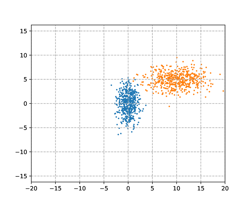
(a) Training data distribution.

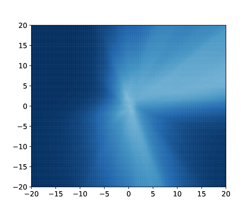
(b) Epistemic Uncertainty estimated by SDE-Net.

Figure 8: Visualization of the epistemic uncertainty estimated by SDE-Net (darker colors represent higher uncertainties in the heat map).

S. 3.2 Expected Calibration Error

In this subsection, we measure the expected calibration error (ECE, (Guo et al., 2017)) to see if the confidences produced by the models are trustworthy. Fig. 9 shows the ECE of each method on MNIST and SVHN. On MNIST, SDE-Net can achieve competitive results compared with DeepEnsemble and MC-dropout and outperforms other methods. On SVHN, SDE-Net outperforms all the baselines.

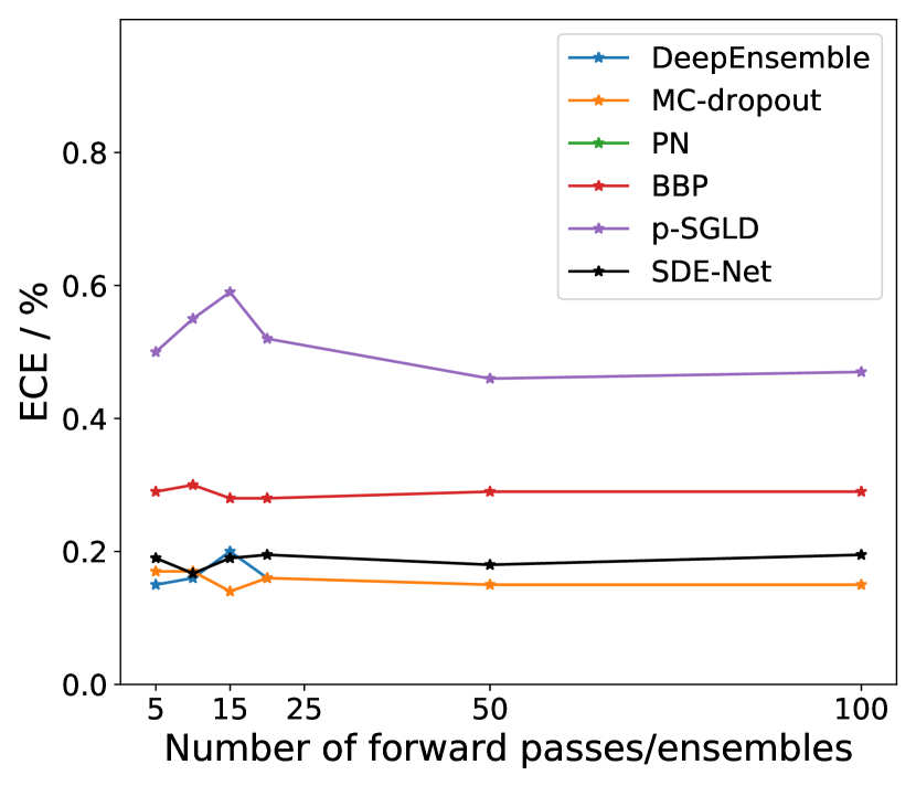
(a) MNIST

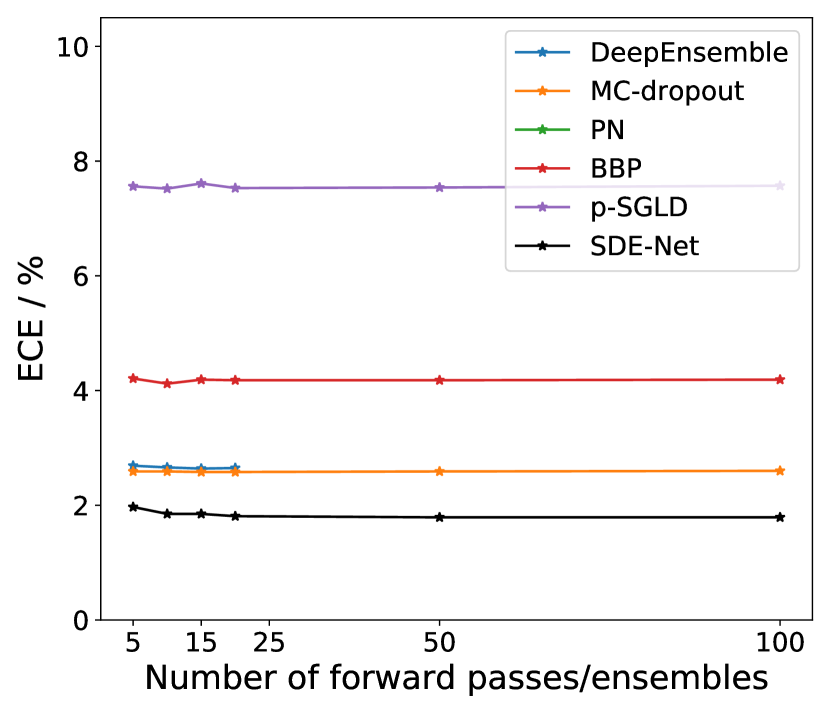
(b) SVHN

Figure 9: Expected calibration error (ECE) vs number of forward passes/ensembles. PN is outside the range and not shown

S. 3.3 Ablation Study

Robustness to different pseudo OOD data. In this set of experiments, we report additional experimental results for OOD detection in classification tasks. We use MNIST as the in-distribution training dataset, and explore using other data sources as OOD data beyond using in-distribution data perturbed by Gaussian noise. The results are shown in Table 4. As we can see, the performance of PN is very poor when using Gaussian noise and training data perturbed by Gaussian noise. When using SVHN as OOD data during training, its performance is good. This suggests that PN is easy to be overfitted by the OOD data used in training. Our SDE-Net can achieve good performance in all settings, which shows its superior robustness.

Table 4: Additional Results for OOD detection. MNIST is used as in-distribution training data. The OOD data used during training is in the bracket beside each model. Gaussian means directly sampling from $\mathcal{N}(0,1)$ as pseudo OOD data. Training+Gaussian means perturbing training data by Gaussian noise (0 mean and variance 4) as pseudo OOD data. SVHN means directly use the training set of SVHN as pseudo OOD data. We report the average performance and standard deviation for 5 random initializations.

OOD Data (test)	Model	TNR at TPR $95\%$	AUROC	Detection accuracy	AUPR in	AUPR out
SVHN	SDE-Net(SVHN)	$99.9\pm 0.0$	$99.9\pm 0.0$	$99.8\pm 0.1$	$99.9\pm 0.0$	$99.9\pm 0.0$
	SDE-Net(Gaussian)	$99.4\pm 0.1$	$99.9\pm 0.0$	$98.5\pm 0.2$	$99.7\pm 0.1$	$100.0\pm 0.0$
	SDE-Net(training+Gaussian)	$97.8\pm 1.1$	$99.5\pm 0.2$	$97.0\pm 0.2$	$98.6\pm 0.6$	$99.8\pm 0.1$
	PN(SVHN)	$100.0\pm 0.0$	$100.0\pm 0.0$	$100.0\pm 0.0$	$100.0\pm 0.0$	$100.0\pm 0.0$
	PN(Gaussian)	$89.0\pm 2.9$	$92.9\pm 1.2$	$92.3\pm 2.2$	$68.1\pm 6.5$	$97.6\pm 0.7$
	PN(training+Gaussian)	$90.4\pm 2.8$	$94.1\pm 2.2$	$93.0\pm 1.4$	$73.2\pm 7.3$	$98.0\pm 0.6$
SEMEION	SDE-Net(SVHN)	$100.0\pm 0.0$	$99.9\pm 0.0$	$99.9\pm 0.0$	$100.0\pm 0.0$	$99.0\pm 0.2$
	SDE-Net(Gaussian)	$99.9\pm 0.1$	$100.0\pm 0.0$	$99.0\pm 0.3$	$100.0\pm 0.0$	$99.8\pm 0.1$
	SDE-Net(training+Gaussian)	$99.6\pm 0.2$	$99.9\pm 0.1$	$98.6\pm 0.5$	$100.0\pm 0.0$	$99.5\pm 0.3$
	PN(SVHN)	$98.0\pm 0.8$	$98.7\pm 0.3$	$97.3\pm 1.2$	$99.6\pm 0.1$	$95.7\pm 2.3$
	PN(Gaussian)	$91.0\pm 2.3$	$94.9\pm 2.6$	$93.2\pm 1.5$	$97.8\pm 0.6$	$86.5\pm 3.5$
	PN(training+Gaussian)	$93.4\pm 2.2$	$96.1\pm 1.2$	$94.5\pm 1.1$	$98.4\pm 0.7$	$88.5\pm 1.3$
CIFAR10	SDE-Net(SVHN)	$100.0\pm 0.0$	$99.9\pm 0.0$	$99.7\pm 0.1$	$99.9\pm 0.1$	$99.8\pm 0.1$
	SDE-Net(Gaussian)	$99.8\pm 0.1$	$100.0\pm 0.0$	$98.9\pm 0.4$	$100.0\pm 0.0$	$100.0\pm 0.0$
	SDE-Net(training+Gaussian)	$99.7\pm 0.2$	$99.9\pm 0.0$	$98.3\pm 0.4$	$99.9\pm 0.0$	$99.9\pm 0.0$
	PN(SVHN)	$100.0\pm 0.0$	$100.0\pm 0.0$	$99.8\pm 0.1$	$100.0\pm 0.0$	$100.0\pm 0.0$
	PN(Gaussian)	$96.8\pm 1.2$	$97.7\pm 0.7$	$96.5\pm 0.6$	$94.3\pm 1.2$	$98.2\pm 0.3$
	PN(training+Gaussian)	$97.6\pm 0.7$	$98.3\pm 0.8$	$97.0\pm 1.2$	$96.0\pm 1.7$	$97.3\pm 1.2$

Table 5: Classification and out-of-distribution detection results on MNIST and SVHN. All values are in percentage, and larger values indicates better detection performance. We report the average performance and standard deviation for 5 random initializations.

ID	OOD	Model	TNR at TPR $95\%$	AUROC	Detection accuracy	AUPR in	AUPR out
MNIST	SEMEION	SDE-Net w.o. reg	$93.7\pm 1.1$	$97.9\pm 0.4$	$95.2\pm 0.9$	$99.8\pm 0.1$	$89.8\pm 1.2$
		SDE-Net	$\bm{99.6}\pm 0.2$	$\bm{99.9}\pm 0.1$	$\bm{98.6}\pm 0.5$	$\bm{100.0}\pm 0$	$\bm{99.5}\pm 0.3$
MNIST	SVHN	SDE-Net w.o. reg	$90.3\pm 1.3$	$96.6\pm 1.3$	$92.2\pm 1.2$	$90.0\pm 2.2$	$98.2\pm 0.4$
		SDE-Net	$\bm{97.8}\pm 1.1$	$\bm{99.5}\pm 0.2$	$\bm{97.0}\pm 0.2$	$\bm{98.6}\pm 0.6$	$\bm{99.8}\pm 0.1$
SVHN	CIFAR10	SDE-Net w.o. reg	$68.2\pm 2.4$	$93.9\pm 0.7$	$90.3\pm 0.9$	$97.2\pm 0.7$	$85.2\pm 1.2$
		SDE-Net	$\bm{87.5}\pm 2.8$	$\bm{97.8}\pm 0.4$	$\bm{92.7}\pm 0.7$	$\bm{99.2}\pm 0.2$	$\bm{93.7}\pm 0.9$
SVHN	CIFAR100	SDE-Net w.o. reg	$65.2\pm 1.3$	$92.9\pm 0.9$	$88.7\pm 0.6$	$97.2\pm 0.3$	$83.4\pm 0.7$
		SDE-Net	$\bm{83.4}\pm 3.6$	$\bm{97.0}\pm 0.4$	$\bm{91.6}\pm 0.7$	$\bm{98.8}\pm 0.1$	$\bm{92.3}\pm 1.1$

Is the OOD regularizer necessary? Our loss objective includes an OOD regularization term which allows us to explicitly train the epistemic uncertainty for each data point. This regularizer can be interpreted as our parameter belief from the data space. That is we want our model to give uncertain outputs for OOD data. To verify the necessity of this regularization term, we test the uncertainty estimates of SDE-Net trained without the regularizer. As we can see from Table. 5, the performance of SDE-Net deteriorates to the same level of traditional NNs without the regularizer term. In Bayesian neural network, the principle of Bayesian inference implicitly enables larger uncertainty in the region that lacks training data. Such inference can be costly and we choose to view the DNNs as stochastic dynamic systems. The benefit of such design is that we can directly model the epistemic uncertainty level for each data point by the variance of the Brownian motion.

S. 3.4 Full Results of Table. 2 and Table. 3 of the main paper

Table. 6 shows the full results of Table. 2 of the main paper.

Table. 7 shows the full results of Table. 3 of the main paper.

Table 6: Out-of-distribution detection for regression on Year Prediction MSD + Boston Housing. We report the average performance and standard deviation for 5 random initializations.

Model	# Parameters	RMSE	TNR at TPR $95\%$	AUROC	Detection accuracy	AUPR in	AUPR out
DeepEnsemble	14.9K$\times 5$	$\bm{8.6}\pm$ NA	$10.9\pm$ NA	$59.8\pm$ NA	$61.4\pm$NA	$99.3\pm$NA	$1.3\pm$ NA
MC-dropout	14.9K	$8.7\pm 0.0$	$9.6\pm 0.4$	$53.0\pm 1.2$	$55.6\pm 1.2$	$99.2\pm 0.1$	$1.1\pm 0.1$
BBP	30.0K	$9.5\pm 0.2$	$8.7\pm 1.5$	$56.8\pm 0.9$	$58.3\pm 2.1$	$99.0\pm 0.0$	$1.3\pm 0.1$
p-SGLD	14.9K	$9.3\pm 0.1$	$9.2\pm 1.5$	$52.3\pm 0.7$	$57.3\pm 1.9$	$99.4\pm 0.0$	$1.1\pm 0.2$
SDE-Net	12.4K	$8.7\pm 0.1$	$\bm{60.4}\pm 3.7$	$\bm{84.4}\pm 1.0$	$\bm{80.0}\pm 0.9$	$\bm{99.7}\pm 0.0$	$\bm{21.3}\pm 4.1$

Table 7: Misclassification detection performance on MNIST and SVHN. We report the average performance and standard deviation for 5 random initializations.

Data	Model	TNR at TPR $95\%$	AUROC	Detection accuracy	AUPR succ	AUPR err
MNIST	Threshold	$85.4\pm 2.8$	$94.3\pm 0.9$	$92.1\pm 1.5$	$99.8\pm 0.1$	$31.9\pm 8.3$
	DeepEnsemble	$89.6\pm$NA	$\bm{97.5}\pm$ NA	$93.2\pm$NA	$\bm{100.0}\pm$ NA	$41.4\pm$ NA
	MC-dropout	$85.4\pm 4.5$	$95.8\pm 1.3$	$91.5\pm 2.2$	$99.9\pm 0.0$	$33.0\pm 6.7$
	PN	$85.4\pm 2.8$	$91.8\pm 0.7$	$91.0\pm 1.1$	$99.8\pm 0.0$	$33.4\pm 4.6$
	BBP	$88.7\pm 0.9$	$96.5\pm 2.1$	$93.1\pm 0.5$	$\bm{100.0}\pm 0.0$	$35.4\pm 3.2$
	P-SGLD	$\bm{93.2}\pm 2.5$	$96.4\pm 1.7$	$\bm{98.4}\pm 0.2$	$\bm{100.0\pm}0.0$	$\bm{42.0\pm}2.4$
	SDE-Net	$88.5\pm 1.3$	$96.8\pm 0.9$	$92.9\pm 0.8$	$\bm{100.0\pm}0.0$	$36.6\pm 4.6$
SVHN	Threshold	$66.4\pm 1.7$	$90.1\pm 0.3$	$85.9\pm 0.4$	$99.3\pm 0.0$	$42.8\pm 0.6$
	DeepEnsemble	$\bm{67.2}\pm$NA	$91.0\pm$ NA	$86.6\pm$ NA	$\bm{99.4}\pm$ NA	$46.5\pm$ NA
	MC-dropout	$65.3\pm 0.4$	$90.4\pm 0.6$	$85.5\pm 0.6$	$99.3\pm 0.0$	$45.0\pm 1.2$
	PN	$64.5\pm 0.7$	$84.0\pm 0.4$	$81.5\pm 0.2$	$98.2\pm 0.2$	$43.9\pm 1.1$
	BBP	$58.7\pm 2.1$	$91.8\pm 0.2$	$85.6\pm 0.7$	$99.1\pm 0.1$	$50.7\pm 0.9$
	P-SGLD	$64.2\pm 1.3$	$\bm{93.0}\pm 0.4$	$\bm{87.1}\pm 0.4$	$\bm{99.4}\pm 0.1$	$48.6\pm 1.8$
	SDE-Net	$65.5\pm 1.9$	$92.3\pm 0.5$	$86.8\pm 0.4$	$\bm{99.4\pm}0.0$	$\bm{53.9}\pm 2.5$

S. 4 Network Architecture

S. 4.1 Classification Task

Downsampling layer:

⬇

#change the in planes to 3 for SVHN

nn.Conv2d(1, dim, 3, 1),

norm(dim),

nn.ReLU(inplace=True),

nn.Conv2d(dim, dim, 4, 2, 1),

norm(dim),

nn.ReLU(inplace=True),

nn.Conv2d(dim, dim, 4, 2, 1),

)

Drift neural network:

⬇

def __init__(self, dim):

super(Drift, self).__init__()

self.norm1 = norm(dim)

self.relu = nn.ReLU(inplace=True)

self.conv1 = ConcatConv2d(dim, dim, 3, 1, 1)

self.norm2 = norm(dim)

self.conv2 = ConcatConv2d(dim, dim, 3, 1, 1)

self.norm3 = norm(dim)

def forward(self, t, x):

out = self.norm1(x)

out = self.relu(out)

out = self.conv1(t, out)

out = self.norm2(out)

out = self.relu(out)

out = self.conv2(t, out)

out = self.norm3(out)

return out

Diffussion neural network for MNIST:

⬇

def __init__(self, dim_in, dim_out):

super(Diffusion, self).__init__()

self.norm1 = norm(dim_in)

self.relu = nn.ReLU(inplace=True)

self.conv1 = ConcatConv2d(dim_in, dim_out, 3, 1, 1)

self.norm2 = norm(dim_in)

self.conv2 = ConcatConv2d(dim_in, dim_out, 3, 1, 1)

self.fc = nn.Sequential(norm(dim_out), nn.ReLU(inplace=True), nn.AdaptiveAvgPool2d((1, 1)), Flatten(), nn.Linear(dim_out, 1), nn.Sigmoid())

def forward(self, t, x):

out = self.norm1(x)

out = self.relu(out)

out = self.conv1(t, out)

out = self.norm2(out)

out = self.relu(out)

out = self.conv2(t, out)

out = self.fc(out)

return out

Diffusion network for SVHN:

⬇

def __init__(self, dim_in, dim_out):

super(Diffusion, self).__init__()

self.norm1 = norm(dim_in)

self.relu = nn.ReLU(inplace=True)

self.conv1 = ConcatConv2d(dim_in, dim_out, 3, 1, 1)

self.norm2 = norm(dim_in)

self.conv2 = ConcatConv2d(dim_in, dim_out, 3, 1, 1)

self.norm3 = norm(dim_in)

self.conv3 = ConcatConv2d(dim_in, dim_out, 3, 1, 1)

self.fc = nn.Sequential(norm(dim_out), nn.ReLU(inplace=True), nn.AdaptiveAvgPool2d((1, 1)), Flatten(), nn.Linear(dim_out, 1), nn.Sigmoid())

def forward(self, t, x):

out = self.norm1(x)

out = self.relu(out)

out = self.conv1(t, out)

out = self.norm2(out)

out = self.relu(out)

out = self.conv2(t, out)

out = self.norm3(out)

out = self.relu(out)

out = self.conv3(t, out)

out = self.fc(out)

return out

ResNet block architecture:

⬇

expansion = 1

def __init__(self, inplanes, planes, stride=1, downsample=None):

super(ResBlock, self).__init__()

self.norm1 = norm(inplanes)

self.relu = nn.ReLU(inplace=True)

self.downsample = downsample

self.conv1 = conv3x3(inplanes, planes, stride)

self.norm2 = norm(planes)

self.conv2 = conv3x3(planes, planes)

def forward(self, x):

shortcut = x

out = self.relu(self.norm1(x))

if self.downsample is not None:

shortcut = self.downsample(out)

out = self.conv1(out)

out = self.norm2(out)

out = self.relu(out)

out = self.conv2(out)

return out + shortcut

For BBP, we use an identical Residue block architecture and a fully factorised Gaussian approximate posterior on the weights.

S. 4.2 Regression Task

The network architecture for DeepEnsemble, MC-dropout and p-SGLD:

⬇

def __init__(self):

super(DNN, self).__init__()

self.fc1 = nn.Linear(90, 50)

self.dropout1 = nn.Dropout(0.5)

self.fc2 = nn.Linear(50, 50)

self.dropout2 = nn.Dropout(0.5)

self.fc3 = nn.Linear(50, 50)

self.dropout3 = nn.Dropout(0.5)

self.fc4 = nn.Linear(50, 50)

self.dropout4 = nn.Dropout(0.5)

self.fc5 = nn.Linear(50, 50)

self.dropout5 = nn.Dropout(0.5)

self.fc6 = nn.Linear(50, 2)

def forward(self, x):

x = self.dropout1(F.relu(self.fc1(x)))

x = self.dropout2(F.relu(self.fc2(x)))

x = self.dropout3(F.relu(self.fc3(x)))

x = self.dropout4(F.relu(self.fc4(x)))

x = self.dropout5(F.relu(self.fc5(x)))

x = self.fc6(x)

mean = x[:,0]

sigma = F.softplus(x[:,1])+1e-3

return mean, sigma

For BBP, we use an identical architecture with a fully factorised Gaussian approximate posterior on the weights.

For SDE-Net:

Drift neural network:

⬇

def __init__(self):

super(Drift, self).__init__()

self.fc = nn.Linear(50, 50)

self.relu = nn.ReLU(inplace=True)

def forward(self, t, x):

out = self.relu(self.fc(x))

return out

Diffusion neural network:

⬇

def __init__(self):

super(Diffusion, self).__init__()

self.relu = nn.ReLU(inplace=True)

self.fc1 = nn.Linear(50, 100)

self.fc2 = nn.Linear(100, 1)

def forward(self, t, x):

out = self.relu(self.fc1(x))

out = self.fc2(out)

out = F.sigmoid(out)

return out

References

- (1) Boston dataset. https://www.cs.toronto.edu/~delve/data/boston/bostonDetail.html.
- Anil et al. (2019) Anil, C., Lucas, J., and Grosse, R. Sorting out lipschitz function approximation. pp. 291–301, 2019.
- Bass (2011) Bass, R. F. Stochastic Processes. Cambridge Series in Statistical and Probabilistic Mathematics. Cambridge University Press, 2011.
- Blundell et al. (2015) Blundell, C., Cornebise, J., Kavukcuoglu, K., and Wierstra, D. Weight uncertainty in neural networks. In International Conference on Machine Learning, pp. 1613–1622, 2015.
- Chen et al. (2018) Chen, T. Q., Rubanova, Y., Bettencourt, J., and Duvenaud, D. K. Neural ordinary differential equations. In Advances in Neural Information Processing Systems, pp. 6571–6583, 2018.
- Choukroun et al. (2016) Choukroun, S., Cosso, A., et al. Backward sde representation for stochastic control problems with nondominated controlled intensity. The Annals of Applied Probability, 26(2):1208–1259, 2016.
- Denker & Lecun (1991) Denker, J. and Lecun, Y. Transforming neural-net output levels to probability distributions. In Advances in Neural Information Processing Systems, pp. 853–859, 1991.
- Dua & Graff (2017) Dua, D. and Graff, C. UCI machine learning repository, 2017. URL http://archive.ics.uci.edu/ml.
- E (2017) E, W. A proposal on machine learning via dynamical systems. Communications in Mathematics and Statistics, 5:1–11, 02 2017.
- Gal & Ghahramani (2015) Gal, Y. and Ghahramani, Z. Bayesian convolutional neural networks with bernoulli approximate variational inference. arXiv preprint arXiv:1506.02158, 2015.
- Gal & Ghahramani (2016) Gal, Y. and Ghahramani, Z. Dropout as a bayesian approximation: Representing model uncertainty in deep learning. In International Conference on Machine Learning, pp. 1050–1059, 2016.
- Geifman et al. (2019) Geifman, Y., Uziel, G., and El-Yaniv, R. Bias-reduced uncertainty estimation for deep neural classifiers. In International Conference on Learning Representations, 2019.
- Gomez et al. (2017) Gomez, A. N., Ren, M., Urtasun, R., and Grosse, R. B. The reversible residual network: Backpropagation without storing activations. In Advances in Neural Information Processing Systems, pp. 2214–2224, 2017.
- Goodfellow et al. (2015a) Goodfellow, I., Shlens, J., and Szegedy, C. Explaining and harnessing adversarial examples. In International Conference on Learning Representations, 2015a.
- Goodfellow et al. (2015b) Goodfellow, I., Shlens, J., and Szegedy, C. Explaining and harnessing adversarial examples. 2015b.
- Guo et al. (2017) Guo, C., Pleiss, G., Sun, Y., and Weinberger, K. Q. On calibration of modern neural networks. In International Conference on Machine Learning, pp. 1321–1330, 2017.
- Hafner et al. (2018) Hafner, D., Tran, D., Lillicrap, T., Irpan, A., and Davidson, J. Noise contrastive priors for functional uncertainty. arXiv preprint arXiv:1807.09289, 2018.
- He et al. (2016) He, K., Zhang, X., Ren, S., and Sun, J. Deep residual learning for image recognition. pp. 770–778, 2016.
- Hendrycks & Gimpel (2017) Hendrycks, D. and Gimpel, K. A baseline for detecting misclassified and out-of-distribution examples in neural networks. In International Conference on Learning Representations, 2017.
- Ince (1956) Ince, E. Ordinary Differential Equations. Courier Corporation, 1956. ISBN 0486603490.
- Kendall & Gal (2017) Kendall, A. and Gal, Y. What uncertainties do we need in bayesian deep learning for computer vision? In Advances in Neural Information Processing Systems, pp. 5574–5584, 2017.
- Kloeden & Platen (1992) Kloeden, P. E. and Platen, E. Numerical solution of stochastic differential equations. Springer-Verlag Berlin, 1992.
- Krizhevsky et al. (2012) Krizhevsky, A., Sutskever, I., and Hinton, G. E. Imagenet classification with deep convolutional neural networks. In Advances in Neural Information Processing Systems, pp. 1097–1105. 2012.
- Lakshminarayanan et al. (2017) Lakshminarayanan, B., Pritzel, A., and Blundell, C. Simple and scalable predictive uncertainty estimation using deep ensembles. In Advances in Neural Information Processing Systems, pp. 6402–6413, 2017.
- Lalley (2016) Lalley, S. P. Stochastic differential equations. In University of Chicago, 2016.
- Larsson et al. (2017) Larsson, G., Maire, M., and Shakhnarovich, G. Fractalnet: Ultra-deep neural networks without residuals. In International Conference on Learning Representations, 2017.
- Lee et al. (2018) Lee, K., Lee, H., Lee, K., and Shin, J. Training confidence-calibrated classifiers for detecting out-of-distribution samples. In International Conference on Learning Representations, 2018.
- Li et al. (2016) Li, C., Chen, C., Carlson, D., and Carin, L. Preconditioned stochastic gradient langevin dynamics for deep neural networks. In AAAI Conference on Artificial Intelligence, pp. 1788–1794, 2016.
- Li et al. (2020) Li, X., Wong, T.-K. L., Chen, R. T., and Duvenaud, D. Scalable gradients for stochastic differential equations. arXiv preprint arXiv:2001.01328, 2020.
- Li (2017) Li, Y. Deep reinforcement learning: An overview. arXiv preprint arXiv:1701.07274, 2017.
- Li et al. (2015) Li, Y., Hernández-Lobato, J. M., and Turner, R. E. Stochastic expectation propagation. In Advances in Neural Information Processing Systems, pp. 2323–2331, 2015.
- Louizos & Welling (2016) Louizos, C. and Welling, M. Structured and efficient variational deep learning with matrix gaussian posteriors. In International Conference on Machine Learning, pp. 1708–1716, 2016.
- Louizos & Welling (2017) Louizos, C. and Welling, M. Multiplicative normalizing flows for variational bayesian neural networks. In Proceedings of the 34th International Conference on Machine Learning-Volume 70, pp. 2218–2227, 2017.
- Lu et al. (2018) Lu, Y., Zhong, A., Li, Q., and Dong, B. Beyond finite layer neural networks: Bridging deep architectures and numerical differential equations. In International Conference on Learning Representations, 2018.
- MacKay (1992) MacKay, D. J. C. A practical bayesian framework for backpropagation networks. Neural Computation, 4(3):448–472, 1992.
- Madry et al. (2018) Madry, A., Makelov, A., Schmidt, L., Tsipras, D., and Vladu, A. Towards deep learning models resistant to adversarial attacks. In International Conference on Learning Representations, 2018.
- Malinin & Gales (2019) Malinin, A. and Gales, M. Reverse kl-divergence training of prior networks: Improved uncertainty and adversarial robustness. In Advances in Neural Information Processing Systems, pp. 14520–14531, 2019.
- Malinin & Gales (2018) Malinin, A. and Gales, M. J. F. Predictive uncertainty estimation via prior networks. In Advances in Neural Information Processing Systems, pp. 7047–7058, 2018.
- Nguyen et al. (2015) Nguyen, A., Yosinski, J., and Clune, J. Deep neural networks are easily fooled: High confidence predictions for unrecognizable images. In IEEE Conference on Computer Vision and Pattern Recognition, pp. 427–436, 2015.
- Pereyra et al. (2017) Pereyra, G., Tucker, G., Chorowski, J., Kaiser, Ł., and Hinton, G. Regularizing Neural Networks by Penalizing Confident Output Distributions. In International Conference on Learning Representations, 2017.
- Platen (1999) Platen, E. An introduction to numerical methods for stochastic differential equations. Acta numerica, 8:197–246, 1999.
- Plessix (2006) Plessix, R.-E. A review of the adjoint state method for computing the gradient of a functional with geophysical applications. Geophysical Journal International, 167:495 – 503, 11 2006.
- Ritter et al. (2018) Ritter, H., Botev, A., and Barber, D. A scalable laplace approximation for neural networks. In International Conference on Learning Representations, 2018.
- Shi et al. (2018) Shi, J., Sun, S., and Zhu, J. Kernel implicit variational inference. In International Conference on Learning Representations, 2018.
- (45) Sun, S., Zhang, G., Shi, J., and Grosse, R. Functional variational bayesian neural networks. In International Conference on Learning Representations.
- Szegedy et al. (2014) Szegedy, C., Zaremba, W., Sutskever, I., Bruna, J., Erhan, D., Goodfellow, I., and Fergus, R. Intriguing properties of neural networks. In International Conference on Learning Representations, 2014.
- Tzen & Raginsky (2019) Tzen, B. and Raginsky, M. Neural stochastic differential equations: Deep latent gaussian models in the diffusion limit. arXiv preprint arXiv:1905.09883, 2019.
- Welling & Teh (2011) Welling, M. and Teh, Y. W. Bayesian learning via stochastic gradient langevin dynamics. In International Conference on International Conference on Machine Learning, pp. 681–688, 2011.
- Wu et al. (2019) Wu, A., Nowozin, S., Meeds, E., Turner, R. E., Hernandez-Lobato, J. M., and Gaunt, A. L. Deterministic variational inference for robust bayesian neural networks. In International Conference on Learning Representations, 2019.
- Zhang et al. (2018) Zhang, G., Sun, S., Duvenaud, D., and Grosse, R. Noisy natural gradient as variational inference. In International Conference on Machine Learning, pp. 5852–5861, 2018.
- Zhang et al. (2017) Zhang, X., Li, Z., Loy, C. C., and Lin, D. Polynet: A pursuit of structural diversity in very deep networks. IEEE Conference on Computer Vision and Pattern Recognition, pp. 3900–3908, 2017.