Constraints on the variation of fine structure constant from joint SPT-SZ and XMM-Newton observations

Abstract

We search for a variation of the electromagnetic fine structure constant ($\alpha\equiv e^{2}/\hbar c$) using a sample of 58 SZ selected clusters in the redshift range ($0.2<z<1.5$) detected by the South Pole Telescope, along with X-ray measurements using the XMM-Newton observatory. We use the ratio of the integrated SZ Compto-ionization to its X-ray counterpart as our observable for this search. We first obtain a model-independent constraint on $\alpha$ of about 0.7%, using the fact that the aforementioned ratio is constant as function of redshift. We then look for logarithmic dependence of $\alpha$ as a function of redshift: $\Delta\alpha/\alpha=-\gamma\ln(1+z)$, as this is predicted by runaway dilaton models. We find that $\gamma$ = $-0.046\pm 0.1$, which indicates that blackthere is no logarithmic variation of $\alpha$ as a function of redshift. We also search for a dipole variation of the fine structure constant using the same cluster sample. We do not find any evidence for such a spatial variation.

I Introduction

Ever since Dirac’s ingenuous argument that Newton’s Gravitational Constant could vary with time Dirac (1937), a number of theories beyond General Relativity and the Standard Model of Particle Physics have predicted the variation of fundamental constants, including the fine-structure constant ($\alpha\equiv e^{2}/\hbar c$) Uzan (2011); Martins (2017). Therefore, a plethora of searches have been undertaken using both laboratory and astrophysical observations to search for variations of $\alpha$. For theories which predict a variation of $\alpha$, Einstein’s equivalence principle is violated in the electromagnetic sector. These theories usually involve coupling between the electromagnetic part of matter fields and scalar fields Bekenstein (1982); Damour and Polyakov (1994); Sandvik et al. (2002); Barrow and Lip (2012).

Another strong impetus in searching for a varying $\alpha$ using different methods, comes from a claimed variation of $\alpha$ using quasar absorption systems Webb et al. (2001) with the Keck/HIRES and VLT/UVES telescopes. Subsequently, the same group also argued for a spatial variation in $\alpha$ at 4.2$\sigma$ significance, which is consistent with a dipole Webb et al. (2011); King et al. (2012). The best-fit position of this dipole is at RA=$(17.5\pm 0.9)$ hr and Declination=$(-58\pm 9)^{\circ}$ Webb et al. (2011); King et al. (2012). However, other groups have failed to confirm this result (eg. Srianand et al. (2004)). blackRecent studies however indicate that this dipole variation could be due to the distortion of the wavelength scale over long wavelength ranges ($\geq 1000$ Å) Whitmore and Murphy (2015). These distortions of the wavelength calibration were demonstrated using asteroid and iodine cell star exposures from both Keck-HIRES and VLT-UVES Whitmore and Murphy (2015), and the aforementioned work also showed that simulated quasar spectra can mimic some of the VLT-UVES features seen in  King et al. (2012), although they cannot explain the Keck-HIRES results. Recently, measurements of zinc and chromium absorption lines in quasars, (which are not sensitive to the aforementioned wavelength distortions) were not consistent with no variations in $\alpha$ within $1\sigma$ Murphy et al. (2016, 2017).

Another motivation in recent years to search for variation in $\alpha$ comes from the Hubble tension conundrum related to the discrepancy in Hubble constant values between the low-redshift and high redshift probes Verde et al. (2019); Bethapudi and Desai (2017). Although current studies indicate that a variation of $\alpha$ can only play a minor role in resolving the Hubble tension Knox and Millea (2020); Hart and Chluba (2020), a variation in $\alpha$ could have implications for this problem.

Therefore, a large number of searches for variations of $\alpha$ have been carried out using a plethora of astrophysical/cosmological probes such as CMB Menegoni et al. (2012); Ade et al. (2015); Hart and Chluba (2018); Smith et al. (2019), Big-Bang Nucleosynthesis Clara and Martins (2020), supermassive black hole at the galactic center Hees et al. (2020), white dwarf spectra  Berengut et al. (2013), strong gravitational lensing Colaço et al. (2020), and also Earth-based measurements using the Oklo natural reactor Damour and Dyson (1996), blackatomic clocks Godun et al. (2014) etc. A recent review summarizing the latest results from all these searches can be found in  Martins (2017) and references therein. All these other searches have come up with null results, and failed to corroborate any claims for a variation in $\alpha$. However, given the positive claim from one group, it is important to continue searching for a variation of $\alpha$ using multiple independent sources, as we continue to gather new data.

Here, we use galaxy clusters in testing for variations in $\alpha$. Galaxy clusters are the most massive, gravitationally collapsed objects in the universe and have proved to be wonderful laboratories for studying cosmology, structure formation, galaxy evolution, neutrino mass, graviton mass, various modified gravity theories etc Allen et al. (2011); Vikhlinin et al. (2014); Desai and Gupta (2020). In the past two decades, a large number of galaxy clusters have been discovered upto very high redshifts thanks to multi-wavelength surveys in optical, X-ray, and Sunyaev-Zeldovich (SZ, hereafter) at mm wavelengths which have mapped out large-area contiguous regions of the universe. The first test for the variation of $\alpha$ using cluster SZ observations was implemented by Galli Galli (2013), who showed that the ratio of integrated Compto-ionization in SZ ($Y_{SZ})$ to its X-ray counterpart ($Y_{X}$) scales as $\alpha^{3.5}$. A limit on the variation of $\alpha$ was obtained from the fact this ratio for the 2011 Early Planck Release Planck Collaboration et al. (2011)) catalog is constant. Holanda et al. (2016a) then showed that the ratio of gas fraction from SZ and X-ray measurements scales as $\alpha^{3}$, after assuming that a variation of $\alpha$ leads to a violation of cosmic distance-duality relation (CDDR)  Etherington (1933). They compared the gas fraction measurements for 29 clusters in the redshift range $0.14<z<0.89$ LaRoque et al. (2006) to constrain $\alpha$ variation at these redshifts. In a follow-up work, Holanda et al Holanda et al. (2016b) combined the angular diameter distance of galaxy clusters along with luminosity distance measurements from type Ia supernovae in the redshift range $0.023<z<0.784$ to constrain variations in $\alpha$. A similar idea was thereafter applied to the combination of gas fraction measurements of Atacama Cosmology Telescope selected clusters in the redshift range $0.12<z<1.36$ and Type Ia supernovae Holanda et al. (2017). Martino et al de Martino et al. (2016) looked for spatial evolution of $\alpha$ from Planck SZ data, by looking for variations in the CMB temperature as a function of redshift at the location of the clusters. Colaco et al Colaço et al. (2019) (C19, hereafter) carried out a similar analysis as in  Galli (2013) by looking for variations in the ratio of $Y_{SZ}$ to $Y_{X}$ as a function of redshift. The main difference with respect to  Galli (2013), is that they assumed (similar to  Holanda et al. (2016a, b); Holanda et al. (2017)) that a variation in $\alpha$ also leads to a violation of the CDDR. Motivated by runaway dilaton models Damour et al. (2002a, b); Martins et al. (2015), C19 thereafter modeled the variation in $\alpha$ as a logarithmic function of the redshift, and used the Planck Early SZ catalog to constrain this variation. All these searches have failed to find any evidence for the variation of $\alpha$.

In this work, we first implement the same procedure as  Galli (2013), to constrain the model-independent variation of $\alpha$. Then, similar to C19, we look for logarithmic variations of $\alpha$ as a function of redshift, by considering South Pole Telescope-selected clusters (with joint X-ray and SZ observations) in the redshift range 0.2 $\leq$ z $\leq$ 1.5. This spans a wider redshift range than in C19, which looked for clusters with $z<0.5$. With the same dataset, we also look for a spatial variation in $\alpha$.

This paper is organized as follows. The basic theory behind the X-ray and SZ observables used for the analysis is presented in Sect. II. Our model for the variation of $\alpha$ is described in Sect. III. The dataset used for our analysis is discussed in Sect. IV. A model-independent constraint on variation of $\alpha$ can be found in Sect. V. Our results for time-varying (using runaway dilaton model) and spatial searches for $\alpha$ can be found in Sect. VI and Sect. VII respectively. We conclude in Sect. VIII.

II Method

The basic observable which we use for this work is the dimensionless ratio of $Y_{SZ}$ to $Y_{X}$ (after suitable scalings). More precise definitions will be given in forthcoming subsections. Both $Y_{SZ}$ and $Y_{X}$ are different proxies for the thermal energy of the cluster and are proportional to cluster mass. blackThey also provide insights on the amount of inhomogeneity and clumping of the intra-cluster medium Planelles et al. (2017). Therefore, studying the relation between the two is important for both astrophysics and cosmology. Consequently, a large number of works Bonamente et al. (2008); Andersson et al. (2011); Bonamente et al. (2012); Rozo et al. (2012, 2014a, 2014b); Liu et al. (2015); Chiu et al. (2018); De Martino and Atrio-Barandela (2016); Biffi et al. (2014); Planelles et al. (2017); Bender et al. (2016); Zhu et al. (2019); Pratt and Bregman (2020); Henden et al. (2018) have studied the scaling relations between $Y_{X}$ and $Y_{SZ}$ using both data and simulations to characterize the systematics in the mass determination as well as any departures from self-similarity. Here, we use this ratio to test for a variation in $\alpha$.

II.1 SZ effect

The thermal SZ effect refers to the distortion in the CMB spectrum due to the inverse Compton scattering between the hot gas present in the intracluster medium and the CMB photons Sunyaev and Zeldovich (1972); Birkinshaw (1999); Carlstrom et al. (2002); Mroczkowski et al. (2019). Since the SZ effect is a spectral distortion, which is independent of redshift, it has become a powerful probe to detect galaxy clusters upto very high redshifts. In the past decade, there have been three primary experiments: South Pole Telescope (SPT) Carlstrom et al. (2011), Atacama Cosmology Telescope Swetz et al. (2011), and the Planck satellite  Planck Collaboration et al. (2016), which have carried out a blind SZ survey to detect galaxy clusters upto very high redshifts. We now discuss how the SZ signal depends on $\alpha$, for which we follow the same outline as in C19.

The distortion measured in SZ experiments is proportional to a parameter, called the Compton parameter $y$, which is given by Birkinshaw (1999); Carlstrom et al. (2002),

$$y=\frac{{\sigma_{T}}k_{B}}{m_{e}c^{2}}\int n_{e}Tdl$$ (1)

Here, $k_{B}$ is the Boltzmann constant, $c$ is the speed of light, $m_{e}$ is mass of the electron, $n_{e}$ is the number density of electrons, $T$ is the electron temperature, and $\sigma_{T}$ is the Thompson scattering cross section which can be written in terms of $\alpha$ as,

$$\sigma_{T}=\frac{8\pi}{3}\left(\frac{\epsilon^{2}}{m_{e}c^{2}}\right)^{2}=\frac{8\pi}{3}\left(\frac{\hbar^{2}\alpha^{2}}{m_{e}^{2}c^{2}}\right)$$ (2)

Now, the integrated Compton parameter $Y_{SZ}$ (over the solid angle of a galaxy cluster) can be written as,

$$Y_{SZ}\equiv\int_{\Omega}y{d\Omega},$$ (3)

where ${d\Omega}=dA/D_{A}^{2}$, blackand $D_{A}$ is the angular diameter distance. Assuming an ideal gas equation of state given by $P=n_{e}k_{B}T$, where $P$ is the pressure of the intracluster medium, one can combine Eq. 1 and Eq. 3 to obtain,

$$Y_{SZ}D_{A}^{2}\equiv\frac{\sigma_{T}}{m_{e}c^{2}}\int PdV$$ (4)

Since $\sigma_{T}\propto\alpha^{2}$ (cf. Eq. 2), we get

$$Y_{SZ}D_{A}^{2}\propto\alpha^{2}.$$ (5)

If we model the variation in $\alpha$ as $\alpha(z)\equiv\alpha_{0}\phi(z)$, where $\alpha_{0}$ is the present value of $\alpha$, the fractional variation in $\alpha$ is given by,

$$\frac{\Delta\alpha}{\alpha_{0}}=\phi(z)-1$$ (6)

Eq. 5 can then be re-written as

$$Y_{SZ}D_{A}^{2}\propto\phi(z)^{2}$$ (7)

II.2 X-rays

At high temperatures, gas present in the intracluster medium emits in X-rays mainly through the thermal bremsstrahlung process Allen et al. (2011). The thermal energy of the gas can be parameterized by the $Y_{X}$ parameter Kravtsov et al. (2006), which can obtained from X-ray surface brightness observations and is given by,

$$Y_{X}=M_{g}(R)T_{X}$$ (8)

where $T_{X}$ is the X-ray temperature of the gas and $M_{g}(R)$ is mass of the gas within the radius $R$. Kravtsov et al Kravtsov et al. (2006) have shown that $Y_{X}$ is strongly correlated with the cluster mass with an intrinsic scatter of about 5-8%, and hence is a very robust proxy for the cluster mass.

The gas mass $M_{g}(R)$ is scales with $\alpha$ as  Gonçalves et al. (2012); Galli (2013); Colaço et al. (2019),

$$M_{g}(<\theta)\propto\phi(z)^{-3/2}D_{L}D_{A}^{3/2},$$ (9)

where $D_{L}$ is the luminosity distance. From Eq. 9, we can see that $M_{g}(R)$ depends upon both $D_{L}$ and $D_{A}$. Both of them are linked by CDDR, $D_{L}=(1+z)^{2}D_{A}$ Etherington (1933). As shown in  Hees et al. (2014); Gonçalves et al. (2020), any variation in $\alpha$ is intertwined with the violation of CDDR, which must be included in any searches for variation of $\alpha$ Colaço et al. (2019). Similar to C19, if we parameterize a violation of CDDR using $D_{L}$ = $\eta(z)$ $(1+z)^{2}$ $D_{A}$, then the variation of $Y_{X}$ scales according to,

$$Y_{X}\propto\phi(z)^{-3/2}\eta(z)$$ (10)

As argued in C19 (and references therein) for modified theories of gravity where the scalar field couples to the electromagnetic sector and breaks the equivalence principle, $\alpha(z)$ is related to $\eta(z)$ according to $\alpha(z)=\eta(z)^{2}$ Colaço et al. (2020); Hees et al. (2014). Therefore, Eq. 10 can be recast as

$$Y_{X}\propto\phi(z)^{-1}$$ (11)

III Model for $\alpha$ variation

The dimensionless ratio of $Y_{SZ}D_{A}^{2}$ to $Y_{X}$ can be combined from Eq. 4 and Eq. 10 Galli (2013)

$$\frac{Y_{SZ}D_{A}^{2}}{Y_{X}}=C_{XSZ}\frac{\int n_{e}(r)T(r)dV}{T(R)\int n_{e}(r)dV},$$ (12)

where

$$C_{XSZ}=\left(\frac{\sigma_{T}}{m_{e}m_{p}\mu_{e}c^{2}}\right)\\ \approx 1.416\times 10^{-19}\left(\frac{Mpc^{2}}{M_{\odot}keV}\right)$$ (13)

The numerator and denominator in Eq. 12 are different proxies for the thermal energy of the cluster. Simulations show that the ratio in Eq. 12 is expected to be a constant with redshift with a scatter of approximately 5-15% Stanek et al. (2010); Fabjan et al. (2011); Kay et al. (2012); Biffi et al. (2014); Planelles et al. (2017). For clusters with isothermal or universal temperature profile Loken et al. (2002), this ratio should be constant with redshift and equal to unity Galli (2013); Colaço et al. (2019). Therefore, assuming no new Physics, there should not be any variation for this ratio as a function of redshift.

Following C19, we combine Eq. 7 and Eq. 11 to rewrite the ratio in Eq. 12 in terms of the variation in $\alpha$ as,

$$\frac{Y_{SZ}D_{A}^{2}}{Y_{X}C_{XSZ}}=C\phi^{3}$$ (14)

where $C$ is an unknown constant, which encapsulates all the cluster astrophysics in the ratio in Eq. 12. A value of $C$ close to one further indicates that the cluster gas has an isothermal profile. Similar to C19 (see also  Holanda et al. (2016a, b); Holanda et al. (2017)), we use runaway dilaton models Damour et al. (2002a, b); Martins et al. (2015) to parameterize the variation in $\phi$ as

$$\phi(z)=1-\gamma\ln(1+z)$$ (15)

In the dilaton model proposed by Damour et al Damour et al. (2002a, b), Eq. 15 was derived by assuming that the velocity of the dilaton field is constant in both matter and dark-energy eras (with different constants for both). With these assumptions, Eq. 15 is valid only in the dark energy dominated era and needs to be augmented by an additional constant term in the matter dominated era. However, De Martinis et al Martins et al. (2015); Martins (2017) have shown that Eq. 15 can also be obtained by directly integrating the Friedman and scalar field equations for the runaway dilaton model, followed by linearizing the field evolution. As pointed out in  Martins et al. (2015), this approximation is valid for low redshifts, but breaks down at large redshifts (close to $z=5$). At these redshifts, the variation with respect to $z$ is model-dependent, depending on the couplings of dilaton field to baryons, dark matter, and dark energy. These variations have been calculated for the different couplings, and can be found in  Martinelli et al. (2017) and can be parametrized by polynomial functions of $z$.

Since our sample extends only to redshift of 1.5, we use Eq. 15 to constrain any putative variation in $\alpha$, as this function has also been used in previous works. However, it is straightforward to extend this analysis to any other parametric model for the variation of $\alpha$. From Eq. 15, the fractional variation in $\alpha$ can be written as

$$\frac{\Delta\alpha}{\alpha}=-\gamma\ln(1+z)$$ (16)

Therefore, the relation in Eq. 14 now becomes

$$\frac{Y_{SZ}D_{A}^{2}}{Y_{X}C_{XSZ}}=C(1-\gamma\ln(1+z))^{3}$$ (17)

We now fit for this relation using the SPT data. blackWe note that we have used $D_{A}$ (needed for evaluating Eq 17) using the Planck 2018 $\Lambda CDM$ cosmological parameters Planck Collaboration et al. (2020) and evaluated using the astropy Astropy Collaboration et al. (2018) module. However, that the Friedman equations themselves get corrections due to the $H^{2}{\phi^{\prime}}^{2}$ term in the presence of a dilaton field Damour et al. (2002a, b); Martins (2017), where the prime indicates the derivative with respect to the logarithm of the scale factor. As shown in  Martins (2017), $\frac{1}{H}\frac{\dot{\alpha}}{\alpha}\sim\frac{\alpha_{had}}{40}\phi^{\prime}$, where $\alpha_{had}$ is the coupling of the dilaton field to hadronic matter. Based on reported limits of $\frac{\dot{\alpha}}{\alpha}<10^{-17}$/yr from atomic clocks Godun et al. (2014), one expects negligible corrections to Friedmann equations from the dilaton couplings, over the redshift range used for the SPT sample. Therefore, it is reasonable to neglect the contribution of the dilaton field to Friedmann equation, and to use the standard Friedmann equation to compute angular diameter distance.

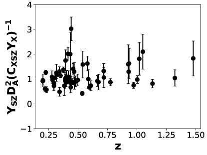
Figure 1: The observed values of $Y_{SZ}$ $D_{A}^{2}$ / $C_{XYZ}$ $Y_{X}$ for the SPT galaxy cluster sample together with X-ray measurements from XMM-Newton observations Bulbul et al. (2019).

IV SPT Cluster Sample

For this work, we use joint X-ray and SZ data for 58 SPT galaxy clusters Bulbul et al. (2019). The SZ data have been obtained by SPT, which is a 10 m telescope at the South Pole, that has imaged the sky at three different frequencies, viz. 95 GHz, 150 GHz and 220 GHz Carlstrom et al. (2011). SPT carried out a 2500 square degree survey between 2007 and 2011 to detect galaxy clusters using the SZ effect. This SPT-SZ survey detected 516 galaxy clusters with mass threshold of $3\times 10^{14}M_{\odot}$ upto redshift of 1.8 Bleem et al. (2015). Detailed properties of the SPT clusters (confirmed until 2015) are discussed in Bleem et al. (2015). Their redshifts have been obtained using a dedicated optical follow-up campaign, consisting of pointed spectroscopic and photometric observations Song et al. (2012); Ruel et al. (2014); Bayliss et al. (2017), and also using data from surveys mapping out contiguous regions of the sky such as BCS Desai et al. (2012) and DES Saro et al. (2015). For every SPT cluster, $Y_{SZ}$ has been estimated by averaging in a cylindrical volume within an aperture radius of 0.75^′  Bleem et al. (2015). These cylindrically averaged $Y_{SZ}$ values for the confirmed SPT clusters are reported in Bleem et al. (2015) and recently updated in  Bocquet et al. (2019). In order to search for a variation of $\alpha$, one needs to compare the $Y_{X}$ measured within a radius $R$, with the $Y_{SZ}$ obtained by averaging over a spherical volume within the same radius $R$ Galli (2013); Holanda et al. (2016a). Since the SPT $Y_{SZ}$ are obtained from cylindrical averaging over an angular aperture of 0.75^′, we first need to convert these values to spherically averaged $Y_{SZ}$ Arnaud et al. (2010) within the same radius at which $Y_{X}$ was measured. To do this conversion we follow the prescription in Arnaud et al. (2010) (see also  Melin et al. (2011)). The cylindrical and spherically averaged $Y$ can be related using:

$$Y_{cyl}(R_{1}) = Y_{sph}(R_{b})-\frac{\sigma_{T}}{m_{e}c^{2}}\int_{R_{1}}^{R_{b}}4\pi P(r)\sqrt{r^{2}-R_{1}^{2}}rdr$$ (18)

$$Y_{sph}(R_{2}) = \frac{\sigma_{T}}{m_{e}c^{2}}\int_{0}^{R_{2}}4\pi P(r)r^{2}dr$$ (19)

where $Y_{cyl}$ is the SZ signal within a cylindrical aperture of radius $R_{1}$; $R_{b}$ is the radial extent of the cluster; and $P(r)$ is the gas pressure in the intra-cluster medium. Similarly, $Y_{sph}$ is the corresponding integrated SZ flux within a sphere of radius $R_{2}$. To do the conversion, we use the Universal Pressure Profile to model $P(r)$ Arnaud et al. (2010). We choose $R_{b}=10R_{500}$. Since the SPT $Y_{X}$ are reported at $R_{500}$ and $Y_{SZ}$ values calculated for an aperture of 0.75^′, we assume $R_{1}=0.75^{\prime}D_{A}$ in Eq. 18 and $R_{2}=R_{500}$ in Eq. 19. Therefore, from Eq. 18 and Eq. 19, we can estimate the ratio of $Y_{sph}(R_{500})$ to $Y_{cyl}(0.75^{\prime}D_{A})$, which is then used to estimate $Y_{sph}(R_{500})$. As pointed out by C19, $Y_{SZ}$ values could also be affected by a modification of the adiabatic evolution of the CMB temperature as a function of redshift. The SPT collaboration has looked for such a violation, and their results are consistent with the standard model of CMB temperature variation with redshift Saro et al. (2014).

SPT has also been undergoing a massive X-ray followup campaign using both the Chandra and XMM-Newton telescopes. Some details of the Chandra-based followups can be found in McDonald et al. (2013, 2014). Previous studies for the scaling relation between SPT $Y_{SZ}$ and $Y_{X}$ (with Chandra measurements) as well as other Physics results have been reported in  Andersson et al. (2011); Semler et al. (2012); McDonald et al. (2013, 2014, 2017); Chiu et al. (2018); McDonald et al. (2019).

Here, we shall use XMM-Newton followup observations of 58 SPT clusters described in Bulbul et al Bulbul et al. (2019). These XMM-Newton observations have been obtained using a combination of targeted X-ray followup programs, led by SPT collaboration members and also other non-SPT based small programs. The redshift range of this sample is given by 0.2 $<$ $z$ $<$ 1.5. The exposure time for each cluster is $\mathcal{O}(10)$ ks. More details of the observations and XMM-Newton data reduction can be found in Bulbul et al. (2019). $Y_{X}$ values for all the 58 clusters have been provided at $R_{500}$ in  Bulbul et al. (2019). blackThe temperatures used for SPT $Y_{X}$ evaluations are emission-weighted temperatures Bulbul et al. (2019). Note that these  Bulbul et al. (2019) provide both the core-excised as well as the core-included $Y_{X}$ data for all the 58 clusters. For our analysis, we combined these blackcore-included $Y_{X}$ estimates along with the spherically averaged $Y_{SZ}$ (converted from those in Bleem et al. (2015)), to construct the ratio $(Y_{SZ}$ $D_{A}^{2}$/ $C_{XYZ}$ $Y_{X})$ as a function of redshift. This variation is shown in Fig. 1. By eye, we see no trends with redshift, thus indicate that the ratio is constant as a function of redshift. We quantify this in the next sections.

V Model-independent constraint

We first report a model-independent constraint on the variation of $\alpha$, along the same lines as Galli Galli (2013), by using the fact that the ratio of SZ to X-Ray Compto-ionization ratio is constant as a function of redshift.

Similar to  Galli (2013), we use the modified weighted least-squares method (MWLS) to calculate the new weighted mean for the ratio and its intrinsic scatter. From the ordinary weighted least-squares method we find from the measurements in Fig. 1 that $\ln(\frac{Y_{SZ}D_{A}^{2}}{Y_{X}C_{XSZ}})=0.05\pm 0.02$, with $\chi^{2}/dof=237/57$. Therefore, using the MWLS, we keep both the weighted mean and the intrinsic scatter as free parameters. For each value of the new weighted mean, the intrinsic scatter is chosen so that the reduced $\chi^{2}$ is equal to one. Among these values, the weighted mean which gives the minimum value for the intrinsic scatter was chosen as the new weighted mean. Using this procedure, we get $\ln(\frac{Y_{SZ}D_{A}^{2}}{Y_{X}C_{XSZ}})=0.046\pm 0.02$, with an intrinsic scatter of 29%. This corresponds to $(\frac{Y_{SZ}D_{A}^{2}}{Y_{X}C_{XSZ}})=1.05\pm 0.02$

The uncertainty in the variation of $\alpha$ is then given by Galli (2013)

$$\frac{\sigma(\alpha)}{\alpha_{0}}=\frac{1}{X}\frac{\sigma(Y_{SZ}D_{A}^{2}/Y_{X}C_{XSZ})}{(Y_{SZ}D_{A}^{2}/Y_{X}C_{XSZ})}$$ (20)

where $X$ is equal to 3 or 3.5, depending on whether the theoretical model for $\alpha$ variation violates CDDR or not. From this we get $\frac{\sigma(\alpha)}{\alpha_{0}}$ $\sim$ 0.7% (violation of CDDR) or 0.6% (no violation of CDDR). This is about the same level of precision as that obtained using the Planck ESZ sample Galli (2013). Similar to  Galli (2013), this limit also assumes no astrophysical evolution of the X-ray to SZ Compto-ionization ratio. However, here we have included the error in cosmological parameters while calculating the observed Compto-ionization ratio, unlike  Galli (2013).

VI Constraints on runaway dilaton models

To look for variations in $\alpha$, we fit the observed ratio (Eq. 14) for the SPT cluster sample to the model in Eq. 17, and obtain the best-fit values of $C$ and $\gamma$ by maximization of the log-likelihood. The log-likelihood function ($\mathcal{L}$) used to test for the variation in $\alpha$ can be written as,

$$-2\ln\mathcal{L}=\sum_{i}\ln 2\pi{\sigma_{i}^{2}}+\sum_{i=1}^{N}\frac{(\phi_{obs,i}-C(1-\gamma\ln(1+z))^{3})^{2}}{\sigma_{i}^{2}}$$ (21)

where $\phi_{obs,i}$ denote the observed values of ratio in Eq. 12 for SPT clusters, $N$ is the total number of clusters, and $\sigma_{i}$ denotes the total error calculated as

$$\sigma_{i}^{2}=\sigma_{\phi}^{2}+\sigma_{int}^{2}$$ (22)

Here, $\sigma_{\phi}$, which is the error in $\phi_{obs,i}$ is obtained by propagating the error in $Y_{X}$, $Y_{SZ}$, and $D_{A}$. We also added an intrinsic scatter term ($\sigma_{int}$) in quadrature, which we keep as a free parameter, while maximizing the log-likelihood. blackWe note that the intrinsic scatter is often added as a free parameter in linear regression problems, since the relation between $y$ and $x$ may not always be 100% deterministic even for noise-free observations, for a variety of reasons Kelly (2007); Hogg et al. (2010). The use of intrinsic scatter is ubiquitous in galaxy cluster astrophysics to quantify how well a given scaling relation is obeyed (eg.  Pratt and Bregman (2020); Liu et al. (2015); Chiu et al. (2020)). A small value for this quantity indicates negligible deviations from the scaling relation and vice-versa. Adding the intrinsic scatter term as a free parameter to the observational errors is similar to the method adopted in  Tian et al. (2020), who used a similar expression to test the tightness of the radial acceleration relation for galaxy clusters. We note however that our treatment of systematic error differs from C19, who used a fixed intrinsic scatter of 17%. For calculating $D_{A}$ and its error, as mentioned earlier, we used the Planck 2018 cosmological parameters Planck Collaboration et al. (2020) ($H_{0}$ = $67.4\pm 0.5$ km/sec/Mpc and $\Omega_{m}$ = $0.315\pm 0.007$).

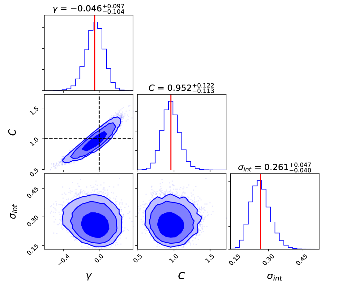
Figure 2: Constraints on $\gamma$ , $C$ (defined in Eq. 14) and $\sigma_{int}$ (defined in Eq. (22)), which are obtained by maximizing the likelihood in Eq. 21 using the emcee module. The plots along the diagonal are the 1-D marginalized likelihood distributions. The red line represents the mean value of the distribution quoted right above the histogram. The off-diagonal plots are the two-dimensional marginalized constraints showing the 68%, 95%, and 99% credible regions, obtained using the Corner module. Our results are consistent with no variation of $\alpha$ and an isothermal profile for clusters.

We maximize the likelihood using the emcee MCMC sampler Foreman-Mackey et al. (2013). The 68%, 95%, and 99% confidence level plots along with the marginalized one-dimensional likelihoods for each of the three parameters are displayed in Fig. 2. The best fits which we get are $\gamma$ = $-0.046_{-0.1}^{+0.097}$ and $C$ = $0.95_{-0.11}^{+0.12}$, with an intrinsic scatter of about 26%. Therefore, our results indicate that there is no evolution of $\gamma$ with redshift, implying no variation in $\alpha$. Furthermore, since the best-fit value of $C$ is consistent with 1.0 within 1$\sigma$ (similar to C19), we conclude that our cluster sample can be adequately described by the isothermal temperature profile.

blackWe note that simulations predict an intrinsic scatter of 5-15% Stanek et al. (2010); Fabjan et al. (2011); Kay et al. (2012); Biffi et al. (2014); Planelles et al. (2017). Our estimated intrinsic scatter of 26% is larger than these estimates. Other observational results for the intrinsic scatter in $Y_{X}-Y_{SZ}$ relation range from negligible scatter of 5% Rozo et al. (2012), to scatters between 15-20% Planck Collaboration et al. (2011); Zhu et al. (2019) which are comparable to our estimate, and also extremely large scatter of 60-90% De Martino and Atrio-Barandela (2016); Pratt and Bregman (2020). These estimates also depend upon the sample used (including significant differences between cool-core and non cool core Zhu et al. (2019)), as well as the regression method employed. We discuss some possible reasons for our large scatter compared to the expectations from simulations.

black Biffi et al. (2014) showed using the MUSIC dataset of simulated clusters that the emission-weighted temperatures show deviations of about 20%, compared to spectroscopic-like or mass-weighted temperatures, which show deviations of only about 10% and 5% respectively. The aforementioned work also showed that the $Y_{X}-Y_{SZ}$ scaling relation shows a scatter of 5% for $Y_{X}$ computed using mass-weighted temperatures, which is comparable to the deviations with respect to the true temperatures. Therefore, one would expect a scatter of about 20%, if $Y_{X}$ was estimated using emission-weighted temperatures. Since the $Y_{X}$ estimates were obtained using the emission-weighted temperatures, that could be one possible reason for our large scatter. Other possibilities could be because of the use of Universal Pressure Profile Arnaud et al. (2010), which is known to overestimate the thermal SZ signal by upto 15-20% depending upon the angular aperture De Martino and Atrio-Barandela (2016). However, a detailed investigation of these and other causes for the large intrinsic will be deferred to future works.

Table. 1 shows the constraints on $\gamma$ from different cosmological observations along with our results. We note that the most stringent bound on $\gamma$ are however obtained from tests of violations of weak equivalence principle and are $\mathcal{O}(10^{-6})$ Martins and Vacher (2019).

Data Set	$\gamma$	Reference
Only Gas Mass Fractions	$+0.065\pm 0.095$	Holanda et al. (2016a)
Angular Diameter Distance + SNe Ia	$-0.037\pm 0.157$	Holanda et al. (2016b)
Gas Mass Fractions + SNe Ia	$+0.010\pm 0.030$	Holanda et al. (2017)
${Y_{SZ}D_{A}^{2}}/{C_{XYZ}Y_{X}}$	$-0.15\pm 0.10$	Colaço et al. (2019)
Strong Gravitational Lensing + SNe Ia	$-0.013_{-0.09}^{+0.08}$	Colaço et al. (2020)
$\mathbf{{Y_{SZ}D_{A}^{2}}/{C_{XYZ}Y_{X}}}$	$\mathbf{-0.046_{-0.104}^{+0.097}}$	This work

Table 1: A summary of the current astrophysical/cosmological constraints from different works (including the result from this work) on a possible time evolution of $\alpha$ for a class of dilaton runaway models ($\phi$ = 1-$\gamma$ $\ln$(1 + $z$)).

VII Search for Dipole variation of $\alpha$

To confirm the dipole variation of $\alpha$ found using quasar data Webb et al. (2011), Galli Galli (2013) also searched for a spatial variation of $\alpha$. Due to their different redshift and spatial distributions compared to quasars, clusters offer a complementary probe to test the claim in  Webb et al. (2011). The model for the dipole variation posited in Galli (2013) is given by

$$\frac{\Delta\alpha}{\alpha}=Arcos(\theta)$$ (23)

where $A$ represents the dipole amplitude, $\theta$ is the angular separation between clusters and best-fit dipole position found in  Webb et al. (2011), $r$ is the lookback time which is given by,

$$r=\int_{0}^{z}\frac{cdz^{{}^{\prime}}}{H(z^{{}^{\prime}})}$$ (24)

For a flat $\Lambda$CDM universe, $H(z^{{}^{\prime}})$ is given by:

$$H(z^{{}^{\prime}})=H_{0}\sqrt{\Omega_{m}(1+z^{{}^{\prime}})^{3}+\Omega_{\Lambda}}$$ (25)

Therefore, Eq. 12 becomes

$$\left(\frac{Y_{SZ}D_{A}^{2}}{Y_{X}C_{XSZ}}\right)^{1/3}=a+brcos(\theta),$$ (26)

where $a$ = $Y_{0}^{1/3}$ and $b$ = $A$ $Y_{0}^{1/3}$; $Y_{0}$ refers to a fixed reference value for $\left(\frac{Y_{SZ}D_{A}^{2}}{Y_{X}C_{XSZ}}\right)$; and $\cos(\theta)$ is the angular position between every SPT cluster and the best-fit dipole position as reported in  Webb et al. (2011). Note that we have $1/3$ in the exponent of Eq. 26, unlike $1/3.5$ in Galli (2013), as we have assumed (similar to the analysis in Sect. VI) that a variation in $\alpha$ also leads to a violation of CDDR. Fig. 3 shows the ratio $\frac{Y_{SZ}D_{A}^{2}}{C_{XYZ}Y_{X}}$ as a function of $rcos(\theta)$ for the SPT cluster sample.

To get the best-fit value of $Y_{0}$ and $A$, we maximize a log-likelihood similar to that in Eq. 21, after including an intrinsic scatter. Again, we have used the emcee MCMC sampler for the optimization. From this analysis, we obtained $Y_{0}$ = $1.0_{-0.045}^{+0.047}$ and $A$ = $-0.003_{-0.003}^{+0.003}$ $(GLy^{-1})$ with an intrinsic scatter of about 26%. The likelihood distributions of our parameters (after assuming violation of CDDR) along with 2-D marginalized contours are displayed in Fig. 4. To compare our results with  Galli (2013), We also repeated our analysis for dipole variation of $\alpha$, assuming no violation in CDDR. So we redid the analysis by replacing the exponent of 3 in Eq. 26 with 3.5. With this assumption, we find $Y_{0}$ = $1.0_{-0.046}^{+0.048}$ and $A$ = $-0.002_{-0.003}^{+0.002}$ $(GLy^{-1})$ with an intrinsic scatter of about 26%. Therefore, our results are also consistent with no dipole variation. A comparison of parameter $A$ with the previous studies in literature is summarized in Table. 2.

Data Set	$A(GLy^{-1})$	Reference
Quasar	($1.1\pm 0.25$) $\times$ $10^{-6}$	Webb et al. (2011)
Planck ESZ Clusters	($-5.5\pm 7.9$ )$\times$ $10^{-3}$	Galli (2013)
SPT Clusters	($\mathbf{-3.0\pm 3.0)\times 10^{-3}}$	This work
SPT Clusters (without CDDR violation)	($\mathbf{-2.0_{-3.0}^{+2.0})\times 10^{-3}}$	This work

Table 2: . A comparison of different studies showing the dipole variation of $\alpha$. We note that the study in  Galli (2013) using Planck ESZ clusters does not assume a violation of CDDR.

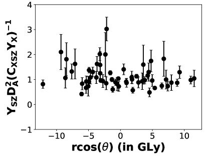
Figure 3: $Y_{SZ}$ $D_{A}^{2}$ / $C_{XYZ}$ $Y_{X}$ as a function of $rcos(\theta)$ for the SPT galaxy cluster sample using XMM-Newton observations Bulbul et al. (2019).

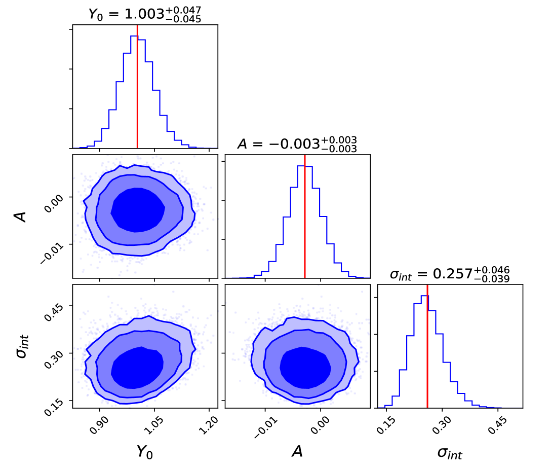
Figure 4: Constraints on $Y_{0}$, $A$ and $\sigma_{int}$ (defined in Eq. 26) used to model a spatial variation in $\alpha$. Eq. 26 assumes that CDDR is also violated when $\alpha$ varies. The plots along the diagonal are the one-dimensional marginalized likelihood distributions. The off-diagonal plots are the two-dimensional marginalized constraints showing the 68%, 95%, and 99% credible regions.

VIII Conclusions

We search for a variation in $\alpha$ as a function of redshift, using the dimensionless ratio of the integrated Compto-ionization to its X-ray counterpart ${Y_{SZ}D_{A}^{2}}/{C_{XYZ}Y_{X}}$. For this study, we use data from 58 SPT-SZ selected galaxy clusters Bleem et al. (2015) in the redshift range 0.2 $\leq$ $z$ $\leq$ 1.5, along with X-ray measurements from XMM-Newton Bulbul et al. (2019). We first do a model-independent test for the variation of $\alpha$ (similar to  Galli (2013)), by using the fact that this ratio is constant as a function of redshift. The variation of $\alpha$ is constrained to within 0.6-0.7% in the redshift range ($0.2<z<1.5$).

Then, similar to C19, we assumed that a variation of $\alpha$ also leads to a violation of cosmic distance duality relation, and parameterized the variation in $\alpha$ as a logarithmic function of redshift and encoded in the parameter $\gamma$ (defined in Eq. 16). This logarithmic variation is characteristic of runaway dilaton models Damour et al. (2002a, b); Martins et al. (2015).

When we fit the $Y_{SZ}$ to $Y_{X}$ ratio for the SPT-SZ data to this model, our best-fit values are given by $\gamma=-0.046_{-0.1}^{+0.097}$ and $C=0.95_{-0.11}^{+0.12}$. Therefore, our results show no significant variation of the $\alpha$ with redshift, in accord with previous results using clusters. Similar to C19, our inferred value of $C$ also indicates that our samples are well approximated by the isothermal temperature profile. A comparison of our results with previous results in literature are summarized in Table 1.

Finally, similar to Galli (2013), we also search for a dipole variation of $\alpha$ with the best-fit direction equal to the value found using quasar-based searches Webb et al. (2011). The model we use to test for dipole variation is given in Eq. 26. Our results show no such spatial variation of $\alpha$, in agreement with previous studies (cf. Table 2).

The first generation SZ surveys from the SPT and ACT telescopes have been superseded by SPTpol, SPT-3G Benson et al. (2014); Bleem et al. (2020) and ACTpol Thornton et al. (2016) respectively, and should detect about an order of magnitude more clusters upto redshift of 2.0. On the X-ray side, the recently launched eROSITA satellite should discover upto 100,000 clusters Hofmann et al. (2017). Therefore, further robust tests of both the temporal and spatial variations of $\alpha$ should soon be possible.

References

- Dirac (1937) P. A. M. Dirac, Nature (London) 139, 323 (1937).
- Uzan (2011) J.-P. Uzan, Living Reviews in Relativity 14, 2 (2011), eprint 1009.5514.
- Martins (2017) C. J. A. P. Martins, Reports on Progress in Physics 80, 126902 (2017), eprint 1709.02923.
- Bekenstein (1982) J. D. Bekenstein, Phys. Rev. D 25, 1527 (1982).
- Damour and Polyakov (1994) T. Damour and A. M. Polyakov, Nuclear Physics B 423, 532 (1994), eprint hep-th/9401069.
- Sandvik et al. (2002) H. B. Sandvik, J. D. Barrow, and J. Magueijo, Phys. Rev. Lett. 88, 031302 (2002), eprint astro-ph/0107512.
- Barrow and Lip (2012) J. D. Barrow and S. Z. W. Lip, Phys. Rev. D 85, 023514 (2012), eprint 1110.3120.
- Webb et al. (2001) J. K. Webb, M. T. Murphy, V. V. Flambaum, V. A. Dzuba, J. D. Barrow, C. W. Churchill, J. X. Prochaska, and A. M. Wolfe, Phys. Rev. Lett. 87, 091301 (2001), eprint astro-ph/0012539.
- Webb et al. (2011) J. K. Webb, J. A. King, M. T. Murphy, V. V. Flambaum, R. F. Carswell, and M. B. Bainbridge, Phys. Rev. Lett. 107, 191101 (2011), eprint 1008.3907.
- King et al. (2012) J. A. King, J. K. Webb, M. T. Murphy, V. V. Flambaum, R. F. Carswell, M. B. Bainbridge, M. R. Wilczynska, and F. E. Koch, Mon. Not. R. Astron. Soc. 422, 3370 (2012), eprint 1202.4758.
- Srianand et al. (2004) R. Srianand, H. Chand, P. Petitjean, and B. Aracil, Phys. Rev. Lett. 92, 121302 (2004), eprint astro-ph/0402177.
- Whitmore and Murphy (2015) J. B. Whitmore and M. T. Murphy, Mon. Not. R. Astron. Soc. 447, 446 (2015), eprint 1409.4467.
- Murphy et al. (2016) M. T. Murphy, A. L. Malec, and J. X. Prochaska, Mon. Not. R. Astron. Soc. 461, 2461 (2016), eprint 1606.06293.
- Murphy et al. (2017) M. T. Murphy, A. L. Malec, and J. X. Prochaska, Mon. Not. R. Astron. Soc. 464, 2609 (2017).
- Verde et al. (2019) L. Verde, T. Treu, and A. G. Riess, Nature Astronomy 3, 891 (2019), eprint 1907.10625.
- Bethapudi and Desai (2017) S. Bethapudi and S. Desai, Eur. Phys. J. Plus 132, 78 (2017), eprint 1701.01789.
- Knox and Millea (2020) L. Knox and M. Millea, Phys. Rev. D 101, 043533 (2020), eprint 1908.03663.
- Hart and Chluba (2020) L. Hart and J. Chluba, Mon. Not. R. Astron. Soc. 493, 3255 (2020), eprint 1912.03986.
- Menegoni et al. (2012) E. Menegoni, M. Archidiacono, E. Calabrese, S. Galli, C. J. A. P. Martins, and A. Melchiorri, Phys. Rev. D 85, 107301 (2012), eprint 1202.1476.
- Ade et al. (2015) P. Ade et al. (Planck), Astron. Astrophys. 580, A22 (2015), eprint 1406.7482.
- Hart and Chluba (2018) L. Hart and J. Chluba, Mon. Not. R. Astron. Soc. 474, 1850 (2018), eprint 1705.03925.
- Smith et al. (2019) T. L. Smith, D. Grin, D. Robinson, and D. Qi, Phys. Rev. D 99, 043531 (2019), eprint 1808.07486.
- Clara and Martins (2020) M. T. Clara and C. J. A. P. Martins, Astron. & Astrophys. 633, L11 (2020), eprint 2001.01787.
- Hees et al. (2020) A. Hees, T. Do, B. M. Roberts, A. M. Ghez, S. Nishiyama, R. O. Bentley, A. K. Gautam, S. Jia, T. Kara, J. R. Lu, et al., Phys. Rev. Lett. 124, 081101 (2020), eprint 2002.11567.
- Berengut et al. (2013) J. C. Berengut, V. V. Flambaum, A. Ong, J. K. Webb, J. D. Barrow, M. A. Barstow, S. P. Preval, and J. B. Holberg, Phys. Rev. Lett. 111, 010801 (2013), eprint 1305.1337.
- Colaço et al. (2020) L. R. Colaço, R. F. L. Holanda, and R. Silva, arXiv e-prints arXiv:2004.08484 (2020), eprint 2004.08484.
- Damour and Dyson (1996) T. Damour and F. Dyson, Nuclear Physics B 480, 37 (1996), eprint hep-ph/9606486.
- Godun et al. (2014) R. M. Godun, P. B. R. Nisbet-Jones, J. M. Jones, S. A. King, L. A. M. Johnson, H. S. Margolis, K. Szymaniec, S. N. Lea, K. Bongs, and P. Gill, Phys. Rev. Lett. 113, 210801 (2014), eprint 1407.0164.
- Allen et al. (2011) S. W. Allen, A. E. Evrard, and A. B. Mantz, Ann. Rev. Astron. Astrophys. 49, 409 (2011), eprint 1103.4829.
- Vikhlinin et al. (2014) A. A. Vikhlinin, A. V. Kravtsov, M. L. Markevich, R. A. Sunyaev, and E. M. Churazov, Physics Uspekhi 57, 317-341 (2014).
- Desai and Gupta (2020) S. Desai and S. Gupta (2020), vol. 1468 of Journal of Physics Conference Series, p. 012003, eprint 1912.05117.
- Galli (2013) S. Galli, Phys. Rev. D 87, 123516 (2013), eprint 1212.1075.
- Planck Collaboration et al. (2011) Planck Collaboration, P. A. R. Ade, N. Aghanim, M. Arnaud, M. Ashdown, J. Aumont, C. Baccigalupi, A. Balbi, A. J. Banday, R. B. Barreiro, et al., Astron. & Astrophys. 536, A11 (2011), eprint 1101.2026.
- Holanda et al. (2016a) R. F. L. Holanda, S. J. Landau, J. S. Alcaniz, I. E. Sánchez G., and V. C. Busti, JCAP 2016, 047 (2016a), eprint 1510.07240.
- Etherington (1933) I. M. H. Etherington, Philosophical Magazine 15, 761 (1933).
- LaRoque et al. (2006) S. J. LaRoque, M. Bonamente, J. E. Carlstrom, M. K. Joy, D. Nagai, E. D. Reese, and K. S. Dawson, Astrophys. J. 652, 917 (2006), eprint astro-ph/0604039.
- Holanda et al. (2016b) R. F. L. Holanda, V. C. Busti, L. R. Colaço, J. S. Alcaniz, and S. J. Landau, JCAP 2016, 055 (2016b), eprint 1605.02578.
- Holanda et al. (2017) R. F. L. Holanda, L. R. Colaço, R. S. Gonçalves, and J. S. Alcaniz, Physics Letters B 767, 188 (2017), eprint 1701.07250.
- de Martino et al. (2016) I. de Martino, C. J. A. P. Martins, H. Ebeling, and D. Kocevski, Universe 2, 34 (2016), eprint 1612.06739.
- Colaço et al. (2019) L. R. Colaço, R. F. L. Holanda, R. Silva, and J. S. Alcaniz, JCAP 2019, 014 (2019), eprint 1901.10947.
- Damour et al. (2002a) T. Damour, F. Piazza, and G. Veneziano, Phys. Rev. D 66, 046007 (2002a), eprint hep-th/0205111.
- Damour et al. (2002b) T. Damour, F. Piazza, and G. Veneziano, Phys. Rev. Lett. 89, 081601 (2002b), eprint gr-qc/0204094.
- Martins et al. (2015) C. J. A. P. Martins, P. E. Vielzeuf, M. Martinelli, E. Calabrese, and S. Pandolfi, Physics Letters B 743, 377 (2015), eprint 1503.05068.
- Planelles et al. (2017) S. Planelles, D. Fabjan, S. Borgani, G. Murante, E. Rasia, V. Biffi, N. Truong, C. Ragone-Figueroa, G. L. Granato, K. Dolag, et al., Mon. Not. R. Astron. Soc. 467, 3827 (2017), eprint 1612.07260.
- Bonamente et al. (2008) M. Bonamente, M. Joy, S. J. LaRoque, J. E. Carlstrom, D. Nagai, and D. P. Marrone, Astrophys. J. 675, 106 (2008), eprint 0708.0815.
- Andersson et al. (2011) K. Andersson, B. A. Benson, P. A. R. Ade, K. A. Aird, B. Armstrong, M. Bautz, L. E. Bleem, M. Brodwin, J. E. Carlstrom, C. L. Chang, et al., Astrophys. J. 738, 48 (2011), eprint 1006.3068.
- Bonamente et al. (2012) M. Bonamente, N. Hasler, E. Bulbul, J. E. Carlstrom, T. L. Culverhouse, M. Gralla, C. Greer, D. Hawkins, R. Hennessy, M. Joy, et al., New Journal of Physics 14, 025010 (2012), eprint 1112.1599.
- Rozo et al. (2012) E. Rozo, A. Vikhlinin, and S. More, Astrophys. J. 760, 67 (2012), eprint 1202.2150.
- Rozo et al. (2014a) E. Rozo, A. E. Evrard, E. S. Rykoff, and J. G. Bartlett, Mon. Not. R. Astron. Soc. 438, 62 (2014a), eprint 1204.6292.
- Rozo et al. (2014b) E. Rozo, J. G. Bartlett, A. E. Evrard, and E. S. Rykoff, Mon. Not. R. Astron. Soc. 438, 78 (2014b), eprint 1204.6305.
- Liu et al. (2015) J. Liu, J. Mohr, A. Saro, K. A. Aird, M. L. N. Ashby, M. Bautz, M. Bayliss, B. A. Benson, L. E. Bleem, S. Bocquet, et al., Mon. Not. R. Astron. Soc. 448, 2085 (2015), eprint 1407.7520.
- Chiu et al. (2018) I. Chiu, J. J. Mohr, M. McDonald, S. Bocquet, S. Desai, M. Klein, H. Israel, M. L. N. Ashby, A. Stanford, B. A. Benson, et al., Mon. Not. R. Astron. Soc. 478, 3072 (2018), eprint 1711.00917.
- De Martino and Atrio-Barandela (2016) I. De Martino and F. Atrio-Barandela, Mon. Not. R. Astron. Soc. 461, 3222 (2016), eprint 1606.04983.
- Biffi et al. (2014) V. Biffi, F. Sembolini, M. De Petris, R. Valdarnini, G. Yepes, and S. Gottlöber, Mon. Not. R. Astron. Soc. 439, 588 (2014), eprint 1401.2992.
- Bender et al. (2016) A. N. Bender, J. Kennedy, P. A. R. Ade, K. Basu, F. Bertoldi, S. Burkutean, J. Clarke, D. Dahlin, M. Dobbs, D. Ferrusca, et al., Mon. Not. R. Astron. Soc. 460, 3432 (2016), eprint 1404.7103.
- Zhu et al. (2019) Y. Zhu, Y.-H. Wang, H.-H. Zhao, S.-M. Jia, C.-K. Li, and Y. Chen, Research in Astronomy and Astrophysics 19, 104 (2019), eprint 1902.07507.
- Pratt and Bregman (2020) C. T. Pratt and J. N. Bregman, Astrophys. J. 890, 156 (2020), eprint 2001.07802.
- Henden et al. (2018) N. A. Henden, E. Puchwein, S. Shen, and D. Sijacki, Mon. Not. R. Astron. Soc. 479, 5385 (2018), eprint 1804.05064.
- Sunyaev and Zeldovich (1972) R. A. Sunyaev and Y. B. Zeldovich, Comments on Astrophysics and Space Physics 4, 173 (1972).
- Birkinshaw (1999) M. Birkinshaw, Physics Reports 310, 97 (1999), eprint astro-ph/9808050.
- Carlstrom et al. (2002) J. E. Carlstrom, G. P. Holder, and E. D. Reese, Ann. Rev. Astron. Astrophys. 40, 643 (2002), eprint astro-ph/0208192.
- Mroczkowski et al. (2019) T. Mroczkowski, D. Nagai, K. Basu, J. Chluba, J. Sayers, R. Adam, E. Churazov, A. Crites, L. Di Mascolo, D. Eckert, et al., Space Science Reviews 215, 17 (2019), eprint 1811.02310.
- Carlstrom et al. (2011) J. E. Carlstrom, P. A. R. Ade, K. A. Aird, B. A. Benson, L. E. Bleem, S. Busetti, C. L. Chang, E. Chauvin, H. M. Cho, T. M. Crawford, et al., PASP 123, 568 (2011), eprint 0907.4445.
- Swetz et al. (2011) D. S. Swetz, P. A. R. Ade, M. Amiri, J. W. Appel, E. S. Battistelli, B. Burger, J. Chervenak, M. J. Devlin, S. R. Dicker, W. B. Doriese, et al., Astrophys. J. Suppl. Ser. 194, 41 (2011), eprint 1007.0290.
- Planck Collaboration et al. (2016) Planck Collaboration, P. A. R. Ade, N. Aghanim, M. Arnaud, M. Ashdown, J. Aumont, C. Baccigalupi, A. J. Banday, R. B. Barreiro, R. Barrena, et al., Astron. & Astrophys. 594, A27 (2016), eprint 1502.01598.
- Kravtsov et al. (2006) A. V. Kravtsov, A. Vikhlinin, and D. Nagai, Astrophys. J. 650, 128 (2006), eprint astro-ph/0603205.
- Gonçalves et al. (2012) R. S. Gonçalves, R. F. L. Holanda, and J. S. Alcaniz, Mon. Not. R. Astron. Soc. 420, L43 (2012), eprint 1109.2790.
- Hees et al. (2014) A. Hees, O. Minazzoli, and J. Larena, Phys. Rev. D 90, 124064 (2014), eprint 1406.6187.
- Gonçalves et al. (2020) R. S. Gonçalves, S. Landau, J. S. Alcaniz, and R. F. L. Holanda, JCAP 2020, 036 (2020), eprint 1907.02118.
- Stanek et al. (2010) R. Stanek, E. Rasia, A. E. Evrard, F. Pearce, and L. Gazzola, Astrophys. J. 715, 1508 (2010), eprint 0910.1599.
- Fabjan et al. (2011) D. Fabjan, S. Borgani, E. Rasia, A. Bonafede, K. Dolag, G. Murante, and L. Tornatore, Mon. Not. R. Astron. Soc. 416, 801 (2011), eprint 1102.2903.
- Kay et al. (2012) S. T. Kay, M. W. Peel, C. J. Short, P. A. Thomas, O. E. Young, R. A. Battye, A. R. Liddle, and F. R. Pearce, Mon. Not. R. Astron. Soc. 422, 1999 (2012), eprint 1112.3769.
- Loken et al. (2002) C. Loken, M. L. Norman, E. Nelson, J. Burns, G. L. Bryan, and P. Motl, Astrophys. J. 579, 571 (2002), eprint astro-ph/0207095.
- Martinelli et al. (2017) M. Martinelli, E. Calabrese, and C. J. Martins, in 14th Marcel Grossmann Meeting on Recent Developments in Theoretical and Experimental General Relativity, Astrophysics, and Relativistic Field Theories (2017), vol. 4, pp. 3664–3669.
- Planck Collaboration et al. (2020) Planck Collaboration, N. Aghanim, Y. Akrami, M. Ashdown, J. Aumont, C. Baccigalupi, M. Ballardini, A. J. Banday, R. B. Barreiro, N. Bartolo, et al., Astron. & Astrophys. 641, A6 (2020), eprint 1807.06209.
- Astropy Collaboration et al. (2018) Astropy Collaboration, A. M. Price-Whelan, B. M. Sipőcz, H. M. Günther, P. L. Lim, S. M. Crawford, S. Conseil, D. L. Shupe, M. W. Craig, N. Dencheva, et al., Astron. J. 156, 123 (2018), eprint 1801.02634.
- Bulbul et al. (2019) E. Bulbul, I. N. Chiu, J. J. Mohr, M. McDonald, B. Benson, M. W. Bautz, M. Bayliss, L. Bleem, M. Brodwin, S. Bocquet, et al., Astrophys. J. 871, 50 (2019), eprint 1807.02556.
- Bleem et al. (2015) L. E. Bleem, B. Stalder, T. de Haan, K. A. Aird, S. W. Allen, D. E. Applegate, M. L. N. Ashby, M. Bautz, M. Bayliss, B. A. Benson, et al., Astrophys. J. Suppl. Ser. 216, 27 (2015), eprint 1409.0850.
- Song et al. (2012) J. Song, A. Zenteno, B. Stalder, S. Desai, L. E. Bleem, K. A. Aird, R. Armstrong, M. L. N. Ashby, M. Bayliss, G. Bazin, et al., Astrophys. J. 761, 22 (2012), eprint 1207.4369.
- Ruel et al. (2014) J. Ruel, G. Bazin, M. Bayliss, M. Brodwin, R. J. Foley, B. Stalder, K. A. Aird, R. Armstrong, M. L. N. Ashby, M. Bautz, et al., Astrophys. J. 792, 45 (2014), eprint 1311.4953.
- Bayliss et al. (2017) M. B. Bayliss, K. Zengo, J. Ruel, B. A. Benson, L. E. Bleem, S. Bocquet, E. Bulbul, M. Brodwin, R. Capasso, I. n. Chiu, et al., Astrophys. J. 837, 88 (2017), eprint 1612.02827.
- Desai et al. (2012) S. Desai, R. Armstrong, J. J. Mohr, D. R. Semler, J. Liu, E. Bertin, S. S. Allam, W. A. Barkhouse, G. Bazin, E. J. Buckley-Geer, et al., Astrophys. J. 757, 83 (2012), eprint 1204.1210.
- Saro et al. (2015) A. Saro, S. Bocquet, E. Rozo, B. A. Benson, J. Mohr, E. S. Rykoff, M. Soares-Santos, L. Bleem, S. Dodelson, P. Melchior, et al., Mon. Not. R. Astron. Soc. 454, 2305 (2015), eprint 1506.07814.
- Bocquet et al. (2019) S. Bocquet, J. P. Dietrich, T. Schrabback, L. E. Bleem, M. Klein, S. W. Allen, D. E. Applegate, M. L. N. Ashby, M. Bautz, M. Bayliss, et al., Astrophys. J. 878, 55 (2019), eprint 1812.01679.
- Arnaud et al. (2010) M. Arnaud, G. W. Pratt, R. Piffaretti, H. Böhringer, J. H. Croston, and E. Pointecouteau, Astron. & Astrophys. 517, A92 (2010), eprint 0910.1234.
- Melin et al. (2011) J. B. Melin, J. G. Bartlett, J. Delabrouille, M. Arnaud, R. Piffaretti, and G. W. Pratt, Astron. & Astrophys. 525, A139 (2011), eprint 1001.0871.
- Saro et al. (2014) A. Saro, J. Liu, J. J. Mohr, K. A. Aird, M. L. N. Ashby, M. Bayliss, B. A. Benson, L. E. Bleem, S. Bocquet, M. Brodwin, et al., Mon. Not. R. Astron. Soc. 440, 2610 (2014), eprint 1312.2462.
- McDonald et al. (2013) M. McDonald, B. A. Benson, A. Vikhlinin, B. Stalder, L. E. Bleem, T. de Haan, H. W. Lin, K. A. Aird, M. L. N. Ashby, M. W. Bautz, et al., Astrophys. J. 774, 23 (2013), eprint 1305.2915.
- McDonald et al. (2014) M. McDonald, B. A. Benson, A. Vikhlinin, K. A. Aird, S. W. Allen, M. Bautz, M. Bayliss, L. E. Bleem, S. Bocquet, M. Brodwin, et al., Astrophys. J. 794, 67 (2014), eprint 1404.6250.
- Semler et al. (2012) D. R. Semler, R. Šuhada, K. A. Aird, M. L. N. Ashby, M. Bautz, M. Bayliss, G. Bazin, S. Bocquet, B. A. Benson, L. E. Bleem, et al., Astrophys. J. 761, 183 (2012), eprint 1208.3368.
- McDonald et al. (2017) M. McDonald, S. W. Allen, M. Bayliss, B. A. Benson, L. E. Bleem, M. Brodwin, E. Bulbul, J. E. Carlstrom, W. R. Forman, J. Hlavacek-Larrondo, et al., Astrophys. J. 843, 28 (2017), eprint 1702.05094.
- McDonald et al. (2019) M. McDonald, S. W. Allen, J. Hlavacek-Larrondo, A. B. Mantz, M. Bayliss, B. A. Benson, M. Brodwin, E. Bulbul, R. E. A. Canning, I. Chiu, et al., Astrophys. J. 870, 85 (2019), eprint 1809.09104.
- Kelly (2007) B. C. Kelly, Astrophys. J. 665, 1489 (2007), eprint 0705.2774.
- Hogg et al. (2010) D. W. Hogg, J. Bovy, and D. Lang, arXiv e-prints arXiv:1008.4686 (2010), eprint 1008.4686.
- Chiu et al. (2020) I. N. Chiu, K. Umetsu, R. Murata, E. Medezinski, and M. Oguri, Mon. Not. R. Astron. Soc. 495, 428 (2020), eprint 1909.02042.
- Tian et al. (2020) Y. Tian, K. Umetsu, C.-M. Ko, M. Donahue, and I. N. Chiu, Astrophys. J. 896, 70 (2020), eprint 2001.08340.
- Foreman-Mackey et al. (2013) D. Foreman-Mackey, D. W. Hogg, D. Lang, and J. Goodman, Publ. Astron. Soc. Pac. 125, 306 (2013), eprint 1202.3665.
- Martins and Vacher (2019) C. J. A. P. Martins and L. Vacher, Phys. Rev. D 100, 123514 (2019), eprint 1911.10821.
- Benson et al. (2014) B. Benson et al. (SPT-3G), Proc. SPIE Int. Soc. Opt. Eng. 9153, 91531P (2014), eprint 1407.2973.
- Bleem et al. (2020) L. E. Bleem, S. Bocquet, B. Stalder, M. D. Gladders, P. A. R. Ade, S. W. Allen, A. J. Anderson, J. Annis, M. L. N. Ashby, J. E. Austermann, et al., Astrophys. J. Suppl. Ser. 247, 25 (2020), eprint 1910.04121.
- Thornton et al. (2016) R. J. Thornton, P. A. R. Ade, S. Aiola, F. E. Angilè, M. Amiri, J. A. Beall, D. T. Becker, H. M. Cho, S. K. Choi, P. Corlies, et al., Astrophys. J. Suppl. Ser. 227, 21 (2016), eprint 1605.06569.
- Hofmann et al. (2017) F. Hofmann, J. S. Sanders, N. Clerc, K. Nandra, J. Ridl, K. Dennerl, M. Ramos-Ceja, A. Finoguenov, and T. H. Reiprich, Astron. & Astrophys. 606, A118 (2017), eprint 1708.05205.