Time-based Handover Skipping
in Cellular Networks: Spatially Stochastic
Modeling and Analysis
Abstract
Handover (HO) management has attracted attention of research in the context of wireless cellular communication networks. One crucial problem of HO management is to deal with increasing HOs experienced by a mobile user. To address this problem, HO skipping techniques have been studied in recent years. In this paper, we propose a novel HO skipping scheme, namely, time-based HO skipping111This work has been presented in part in [1].. In the proposed scheme, HOs of a user are controlled by a certain fixed period of time, which we call skipping time. The skipping time can be managed as a system parameter, thereby enabling flexible operation of HO skipping. We analyze the transmission performance of the proposed scheme on the basis of a stochastic geometry approach. In the scenario where a user performs the time-based HO skipping, we derive the analytical expressions for two performance metrics: the HO rate and the expected data rate. The analysis results demonstrate that the scenario with the time-based HO skipping outperforms the scenario without HO skipping particularly when the user moves fast. Furthermore, we reveal that there is a unique optimal skipping time maximizing the transmission performance, which we obtain approximately.
Index Terms:
Cellular networks, mobility, handover skipping, handover rate, data rate, stochastic geometry.I Introduction
I-A Background and Motivation
The development of fifth generation (5G) wireless cellular communication systems is driven by the need to satisfy the ever-increasing capacity demand resulting from the proliferation of mobile phones, tablets, and other handheld mobile devices. One of the key features of the 5G evolution is network densification through small cell deployment [2]. Densifying base stations (BSs) shrinks the service area of each BS, increases spectral efficiency, and offers more capacity, thereby enabling a significant increase in the quality of service. However, deploying more BSs promotes frequent handovers (HOs), which increase the risk of disconnection and signaling overhead. Therefore, countermeasures against the problem of frequent HOs are under discussion upon conducting network densification.
The problem of frequent HOs has been addressed by means of HO skipping [3, 4, 5, 6, 7, 8, 9], which is a technique whereby some HOs of a moving user are skipped to reduce excessive HOs. This approach is particularly effective when the user moves fast, or the network consists of densified small cells. The HO skipping enables a user to reduce the HO rate, whereas it may decrease the data reception rate (data rate) because it demands the user to maintain longer connection duration with a BS. Thus, the HO skipping presents a trade-off relation between the increased HO rate and the decreased data rate, and the trade-off relation should be balanced to improve transmission performance of users. Accordingly, a reliable framework for analyzing the trade-off relation is needed to evaluate the HO skipping. In this paper, we propose a novel HO skipping scheme, namely, time-based HO skipping, and provide an analysis framework for the two metrics, the HO rate and the expected data rate.
I-B Related Work
I-B1 HO Management
To suppress frequent HOs, HO management for mobile users has been considered. This management has recently attracted attention in the context of cellular networks (see, e.g., [10] for a survey). Zahran et al. [11] proposed an application-specific signal threshold adaptation scheme to reduce excessive HOs. In the scheme, they established an algorithm for HO management by considering the received signal strength and estimated life time. Zhang et al. [12] proposed an algorithm for reducing HO signaling overhead. However, BS intensity and interference signals from other BSs are not considered in their analysis. In addition, none of these studies describe the trade-off relation between increased HO rate and decreased data rate. Ylianttila et al. [13] proposed dwell timer schemes for HO management, and they considered the trade-off relation to find the optimal HO frequency that improves the transmission performance. However, their study is based on simulations, and an analytical framework for evaluating the trade-off is not considered.
I-B2 HO Rate and Data Rate Analysis
To investigate the effect of HOs on the transmission performance, the HO rate and the data rate are essential metrics. Motivated to provide mathematical studies for these metrics, theory of spatial point processes and stochastic geometry has been adopted to model cellular networks. Baccelli and Zuyev [14] first analyzed the HO rate by a stochastic geometry approach. By modeling the BS locations in a cellular network with a homogeneous Poisson point process (PPP), they derived analytical expressions for the distribution of the number of HOs during a fixed period of time when a user moves along a straight line. Lin et al. [15] proposed a modified random waypoint (RWP) model to describe user mobility. By applying this model to homogeneous networks where BSs are arranged according to a hexagonal grid or a homogeneous PPP, they derived analytical results of the HO rate and the expected sojourn time in a typical BS cell. However, the above results do not consider the data rate.
Regarding data rate analysis by a stochastic geometry approach, Andrews et al. [16] first analyzed the data rate and coverage focusing on signal-to-interference-plus-noise ratio (SINR) distribution in the context of cellular networks. They derived the analytical expressions of the coverage probability and the expected downlink data rate of a typical user in a single-tier homogeneous cellular network. Renzo et al. [17] analyzed the downlink data rate of a typical user under generalized assumptions on the fading effect. However, the above studies assume that the typical user is static, and therefore they did not consider HOs. Analyzing the trade-off relation between increased HO rate and decreased data rate are crucial for evaluating the transmission performance of moving users.
Several works studied the trade-off through analyzing the HO rate and the data rate. Bao and Liang [18] considered a multi-tier heterogeneous network configured by overlaid independent homogeneous PPPs and derived the exact expressions of the intra- and inter-tier HO rates for a user moving on an arbitrary trajectory. In addition, they proposed an optimal tier selection by balancing the HO rate and the expected downlink data rate. Another study of Bao and Liang [19] considered BS cooperated cellular networks, and they provided analytical expressions for the HO and expected downlink data rates. In addition, they proposed the optimal cooperating strategy by maximizing an evaluation function consisting of those two metrics. Chattopadhyay et al. [20] considered maximizing throughput in a two-tier network, where multiple moving users and static users are connected to either of macro or micro BSs. They found the optimal proportion of macro and micro BSs density and their respective transmit power levels by balancing the HO rate of the moving users, the expected downlink data rate of the moving and static users, and the expected number of the users connected to a BS, any of which are analytically described.
Some related works considered a trade-off relation between HO rate and coverage. Sadr and Adve [21] considered the HO rate in multi-tier heterogeneous cellular networks and analyzed the negative effect of performing HOs on the coverage. Using the analysis results, they derived the optimal proportion of the BS densities in different tiers to maximize the coverage.
I-B3 Analysis of HO Skipping
HO skipping is an approach to reduce excessive HOs, performing HOs only when a certain predefined condition is satisfied and skipping HOs otherwise. By doing so, it aims to balance the relation between HO rate and data rate. Due to the effectiveness, many HO skipping schemes have recently been proposed, and some of the works successfully provided analytical frameworks for HO skipping schemes via stochastic geometry. A fundamental HO skipping scheme, which we call alternate HO skipping, was introduced by Arshad et al. [3]. In this scheme, a user alternately performs HOs along its trajectory, thereby achieving a 50% reduction in the HO rate. Moreover, they analyzed the negative effect of the alternate HO skipping on the downlink data rate, that is, the impact of the prolonged connection duration with a BS due to the alternate HO skipping. Using these results, they evaluated user throughput by constructing an evaluation function, which represents the trade-off between increase in HO rate and decrease in data rate. It was demonstrated that the user throughput can be improved at least when either the moving speed of a user or the BS density is sufficiently high. The work [3] was extended in [4] and [5]; [4] introduced the alternate HO skipping in two-tier networks and [5] introduced it in a BS cooperating network with coordinated multi-point (CoMP) transmission. Another HO skipping scheme, called topology-aware HO skipping, was proposed in [6]. In this scheme, the HO skipping is triggered according to the user’s distance from the target BS and the size of the cell; that is, HOs are not performed when the user enters a cell whose area is smaller than a certain threshold, or a cell whose dominant BS is farther from the user than a certain threshold. Thus, the topology-aware HO skipping can prevent the connection distances from being unnecessarily long. However, this scheme was evaluated by Monte Carlo simulations, and no mathematical framework for the performance evaluation was presented. The mathematical framework for evaluating topology-aware HO skipping was provided by Demarchou et al. [7]. They derived the analytical expressions of the coverage probability and the expected downlink data rate when the topology-aware HO skipping is performed under the assumption that the trajectory of a moving user is a straight line. They also proposed an HO skipping scheme that is suited to a user-centric CoMP scheme. However, both the alternate and the topology-aware HO skippings do not consider the connection duration, i.e., the communication time connecting to a BS until the next HO. Such connection duration is essential for the HO management due to the problem of signaling overhead. More precisely, when a user performs an HO, its data transmission is temporarily disrupted during the signaling procedure of the HO. This sudden disruption causes unwanted delay and may significantly degrade the performance of network applications. Thus, keeping connection for a certain duration is important for the communication quality of ultra-reliable applications, e.g., high-quality video streaming services and vehicular safety applications. Owing to the above reason, an HO skipping scheme that can control the connection duration needs developing.
I-C Contribution of This Study
In this paper, we propose a novel HO skipping scheme, time-based HO skipping. Our proposed scheme considers a threshold of time, which we call the skipping time, to control the frequency of HOs for a moving user; that is, all HOs attempted earlier than the threshold are skipped, and a user is guaranteed to keep connected during this threshold time. By adjusting the skipping time, our proposed scheme enables to directly control the connection duration of the user with a BS. We provide a tractable framework for analyzing the time-based HO skipping scheme. Under a random walk model of user mobility, we derive the analytical expressions of the HO rate and the expected downlink data rate when the user performs the time-based HO skipping. Moreover, by using these two metrics, we construct an evaluation function of the transmission performance of a moving user, regarding the trade-off relation between the HO rate and the data rate. On the basis of this evaluation function, we conduct a performance comparison between two scenarios: (1) the non-skipping scenario where the moving user do not perform any HO skipping and experience HOs whenever they cross the boundaries of BS cells, and (2) the HO skipping scenario where the moving user perform the time-based HO skipping. The results indicate that the difference of the performance in these two scenarios depends on the speed of the moving user; the non-skipping scenario is better when the user moves slow, whereas the HO skipping scenario is better when the user moves fast. In addition, we maximize the evaluation function by controlling the skipping time of the time-based HO skipping scheme. We also investigate the relation among the optimal skipping time that maximizes the evaluation function and the other system parameters in our model. Furthermore, we attempt to derive an approximate expression of the optimal skipping time. This paper gives much enhancement of [1]; enriched analysis results are provided compared with [1], and the optimal skipping time is newly found in this paper. All the results of this paper are verified by numerical experiments.
I-D Paper Organization
The rest of the paper is organized as follows. In Section II, we describe the network and user mobility models, propose the time-based HO skipping scheme, and define the evaluation function of the transmission performance. The analyses of the HO rate and the data rate are provided in Section III. In Section IV, we evaluate the transmission performance with numerical experiments, and consider maximizing the transmission performance with respect to the skipping time in numerical and analytical ways. Finally, the paper is concluded in Section V.
II System Model
II-A Network Model
We consider a homogeneous cellular network where all BSs transmit signals with the same power level (normalized to 1) utilizing a common spectrum bandwidth. We adopt the conventional assumption that the BSs are arranged according to a homogeneous PPP on with intensity (), where the points of are numbered in an arbitrary order, and we assume that a user equipment (UE) receives downlink signals from one of the allocated BSs. We also assume Rayleigh fading and power-law path-loss on the downlinks but ignore shadowing effects; that is, when a UE at a position receives a signal from the BS located at , , at time (), the received signal power is represented by , where , are mutually independent and exponentially distributed random variables with unit mean () representing the fading effects, and () denotes the path-loss exponent. Here, denotes the Euclidean norm.
We suppose that each UE is initially associated with the nearest BS; that is, the BS cells form a Poisson–Voronoi tessellation. Owing to the stationarity of the network model, there is no loss of generality in focusing on a UE that is assumed to be at the origin at time zero; we refer to this UE as the typical UE. Let denote the index of the nearest point of to the origin; that is, for all . Then, the probability density function of is given as follows, (see, e.g., Sec. 2.3 of [22])
| (1) |
We further suppose that the UEs move on the two-dimensional plane, and a BS transmits a signal to each of its serving UEs at every unit of time. When the typical UE is at a position at time and is associated with the BS at , the downlink SINR of this UE is represented by
| (2) |
where denotes a positive constant representing the noise power, and denotes the interference power to the typical UE given by
| (3) |
Then, , the expected downlink data rate when the UE is associated with at a position at time , is defined as
| (4) |
II-B Mobility Model with Time-based HO Skipping
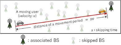
We describe the time-based HO skipping scheme performed in a mobility model for a moving UE. First, we introduce a parameter as the skipping time of the typical UE and assume that the typical UE skips to perform HOs for the skipping time ; that is, the typical UE is allowed to perform an HO every units of time only. We refer to each period of the skipping time as a movement period. Fig. 1 illustrates the typical UE moving straightly for a movement period. We note that the UE is not always associated with the closest BS during the movement period, and the expected distance between the UE and its associated BS becomes larger as the skipping time becomes larger. Whereas, the UE is associated with the closest BS in the end of the movement period since the UE can perform HOs at the endpoint.
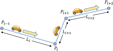
We next give a simple and tractable random walk model to describe mobility of the typical UE. We recall that the typical UE is at the origin at time zero. Let denote a sequence of independent and identically distributed (i.i.d.) random variables on . Then, the position of the typical UE after movement periods is given by the two-dimensional random walk
with . We assume that the typical UE moves on the line segment at a constant velocity during each movement period; that is, the velocity during the -th movement period is equal to for . A trajectory of the typical UE is shown in Fig. 2.
This random walk model is a flexible mobility model that can capture various mobility patterns by choosing the distribution of . Let denote the polar coordinates of . The distributions of and respectively represent the variation of a moving distance, and a direction change of the UE in the -th movement period. Note that the distance corresponds to the moving speed of the UE in the -th movement period since we consider the common moving time in every movement period. For instance, represents that the UE can take a pause in units of time. Furthermore, if is a constant, the UE always moves in a straight line.
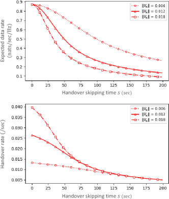
We consider the expected data rate and the HO rate of the typical UE in this model of the time-based HO skipping scheme. Fig. 3 shows numerical examples of the expected data rate and the HO rate of the UE attempting the time-based HO skipping with skipping time , which are based on the analysis in the next section. In this example, there are three parameter patterns as follows: (km/s), which denotes the speed of the UE moving in the -th movement period. It can be seen that the expected data rate decreases as the skipping time becomes large. This is because the UE moves to a further position from the origin as becomes larger, so that the expected data rate becomes smaller when the UE fixes its associated BS. On the other hand, it can also be seen that the HO rate decreases as increases. Intuitivelly, this is because at most one HO occurs during a movement period of time so that the HO rate, that is the expected number of performed HOs divided by , decreases as increases.
To conduct comparison studies to evaluate the time-based HO skipping scheme, we consider two scenarios; Scenario 1 is the non-skipping scenario: the typical UE does not attempt HO skipping and performs HOs whenever the typical UE crosses the boundaries of cells. Scenario 2 is the time-based HO skipping scenario: the typical UE attempts the time-based HO skipping in every movement period.
II-C Evaluation Function of Transmission Performance
We define an evaluation function of transmission performance of a moving UE, so that the evaluation function represents the trade-off between increase in HO rate and decrease in data rate. Let and , , denote the expected amounts of received data and the expected number of HOs for the typical UE moving through a distance for time in Scenario , respectively. We note that corresponds to the skipping time, and corresponds to a moving distance during a movement period. Using these expressions, we define the transmission performance in the respective scenarios as follows:
| (5) |
where is a cost factor that transforms an HO into the amount of lost data by conducting the HO222As described in Section I, there are some risks of performing HOs such as the disconnection and the signaling overhead. In our model, such risk factors of HOs are transformed to the amount of lost data by the constant .. We note that , , denotes the data rate, whereas denotes the HO rate for Scenario . We also note that is not greater than one, namely, the HO rate in Scenario 2 is not greater than . This is due to the assumption that at most one HO occurs during the period of time in Scenario 2. Therefore, the term that has a negative impact on the performance of HOs are almost negligible in Scenario 2 when is sufficiently large.
III Handover Rate and Data Rate Analysis
In this section, we analyze the transmission performance of a moving UE. We investigate the HO rate and the expected downlink data rate for the typical UE in Scenarios 1 and 2 described in the preceding section. We note that in Scenario 2, if the typical UE has crossed one or more boundaries of BS cells in a movement period, then it experiences an HO at the end of the period and is associated with the nearest BS from the new position. Throughout this section, we focus only on the first movement period and fix the movement of the typical UE as for ; that is, the typical UE starts from the origin and moves to in units of time.
III-A Handover Rate Analysis
By the definition, is evaluated as the expected number of intersections of a line segment of length and the boundaries of Poisson–Voronoi cells. On the other hand, is evaluated as the probability that a line segment of length has one or more intersections with the boundaries of Poisson–Voronoi cells because at most one HO occurs in a movement period of a distance . As described in Remarks 1 and 2 below, the analytical expressions of and are both obtained from the existing results. For this reason, we leave the proofs to the references, and introduce only the results of these expressions of and .
III-A1 Handover Rate Analysis for Scenario 1
The HO rate in Scenario 1, that is the non-skipping scenario, is given as follows.
Proposition 1
The expected number of HOs in the non-skipping scenario is given by
| (6) |
III-A2 Handover Rate Analysis for Scenario 2
The HO rate in Scenario 2, that is the time-based HO skipping scenario, is given as follows.
Proposition 2
The expected number of HOs in the time-based HO skipping scenario is given by
| (7) |
where
| (8) |
with
| (9) |
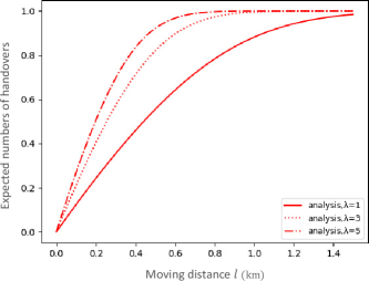
Remark 2
Fig. 4 shows numerically computed results of in (7). It can be seen that the expected number of HOs becomes larger when the intensity of BSs becomes larger. This is because a UE tends to cross more cell boundaries as BSs are more densified. Besides, the expected number of HOs asymptotically approaches to , since a UE surely crosses the boundary at least once when the UE moves through sufficiently long distance.
III-B Data Rate Analysis
We now consider and , the expected amount of data received by the typical UE per movement period in Scenario 1 and Scenario 2, respectively. We note that in Scenario 1, the typical UE is always associated to the nearest BS during a movement period, whereas the UE is not always associated to the nearest BS in Scenario 2. We recall that the movement period is through a distance for units of time.
III-B1 Data Rate Analysis for Scenario 1
First, we provide an expression for , which is derived by applying Theorem 3 in [16].
Theorem 1
The expected amount of received data in the non-skipping scenario is given by
| (10) |
where
| (11) |
with
Proof:
We assume that the typical UE is at a position , , on the trajectory at time . We recall that () is defined as discrete time in our model, and note that because the speed is constant in a movement period. Let denote the index of the nearest BS from the position , and let . Then, by (2) and (4), the data rate per unit time received at the position is given by
| (12) |
and we have
| (13) |
Since the point process is stationary (the distribution is invariant under translations), the distribution of is identical to that of . Furthermore, since , , , are i.i.d., and therefore in (12) are identically distributed for any . Thus, (13) reduces to
The expectation on the right-hand side above is the expected data rate per unit of time considered in Theorem 3 of [16]. Hence, by the conventional way (c.f. [16], [23]), we obtain (10) with (11). ∎
Remark 3
Theorem 1 implies that when a moving UE is always associated with its nearest BS, the expected amount of received data in units of time equals to times the expected data rate for a static UE, which is followed by the stationarity assumption. A similar description is found in Remark 2 of [20]. For this reason, does not depend on the moving distance , that is, .
III-B2 Data Rate Analysis for Scenario 2
By contrast to Scenario 1, a different situation is observed in Scenario 2, where a UE is not always associated with its nearest BS but remains associated with the BS that is the nearest to the starting point.
Theorem 2
The expected amount of received data in the time-based HO skipping scenario is given by
| (14) |
where
| (15) |
with
where and are given in (9).
Proof:
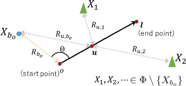
As in the proof of Theorem 1, we suppose that the typical UE is at a position , , on the trajectory at time . We recall that denotes the nearest point of to the origin. Let denote the polar coordinate of . Then, the distance from the typical UE to is given by
where we should note that . An example image of the arrangement of the UE, , and (), is shown in Fig. 5.
The data rate per unit time received at the position is given by
| (16) |
and we have
| (17) |
We note that the following equality holds from (14) and (17),
That is, in (15) corresponds to the expected data rate per unit of time for a UE at the position when the UE is associated with the nearest BS to the origin.
As in (1) and , we have
| (18) |
where is given in (9). Note here that due to the assumption of Rayleigh fading. Then, applying Lemma 1 of [23] to the conditional expectation with respect to the event yields
| (19) |
where the Laplace transform of is applied in the last equality. Furthermore, the interference expression in (3) leads to
| (20) |
where we use the Laplace transform of , , in the second equality, and the third equality follows from the Laplace functional of a homogeneous PPP (see, e.g., Chap. 4 in [22]). We note that in the third equality is given in (9) as well as .
We note that, in contrast to Scenario 1, in Theorem 2 is a function of because it depends on the speed of a UE.
Theorem 2 provides the exact expression of the data rate in Scenario 2; however, the obtained expression is rather complex. If we are allowed to introduce an approximation, we can derive another simpler expression under the interference-limited assumption.
Corollary 1
If we assume , that is, noise power is negligible, then in (15), the expected data rate in the time-based HO skipping scenario at the position , , is approximately given by
| (21) |
where
| (22) |
Proof:
Note that in (20), the Laplace functional of PPP is considered under the condition that there are no points of inside the circle region . Here, we ignore this condition and apply the Laplace functional of a homogeneous PPP over entire . Then,
| (23) |
Substituting in the integral above, we have
| (24) |
Substituting (III-B2), (20), (III-B2), and (III-B2) into (III-B2), using (9), and assuming , we have
where is given in (22). Then, we can apply the following formula to the expression above:
and the result follows. ∎
Remark 4
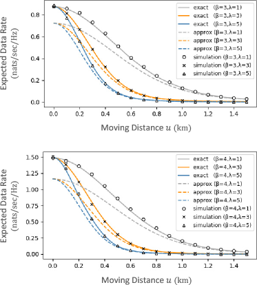
Fig. 6 shows a comparison among the numerically computed in (15), in (21), and the mean of 10,000 independent samples of in (16) computed by Monte Carlo simulation. We see that the analytical result of surely corresponds to the simulation. On the other hand, the analytical result of has some gaps from the result of , particularly when the moving distance of the UE is small. However, these gaps tend to be small as the moving distance becomes large. This is because the distance from the UE to the points of in becomes large as the moving distance increases, and therefore the effect of the approximation becomes weak. Furthermore, it can be seen that the expected data rate is smaller when the BS density is larger or the path loss exponent is smaller, even for the same moving distance . This is because the interference power increases as increases or decreases.
Corollary 1 provides a simple form for calculating the data rate in Scenario 2; however, as shown in Fig. 6, the introduced approximation causes some errors, particularly when a UE is close to the starting point (i.e., ). Nevertheless, since can be calculated exactly by Theorem 1, we can refine the approximate formula by using . Accordingly, we propose a refined version of Corollary 1 as follows.
Corollary 2
Remark 5
We note that the form in (25) takes its value between and , and the balance of the weight between the two metrics is gradually inclined from the former to the latter as becomes large. The degree of the incline is adjusted by the fitting parameter . This refines the error in (21) because , and for sufficiently large , where we recall that tends to be exact as becomes large.
Fig. 7 shows numerically computed values of the expected data rate at based on three different values of in (15), in (21), and in (25), compared with the simulation result. We set the fitting parameter as . It can be seen that the curve of is closer to the exact result than the approximation result .
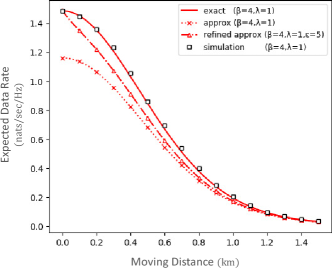
As described above, in (25) provides well-accurate result of the data rate in Scenario 2 with less computational complexity, although the parameter needs fitting for and . In contrast, such fitting is not needed for in (15) and in (21), whereas the former has serious computational complexity, and the latter has some errors from the exact result.
IV Evaluation of Transmission Performance
In this section, we study the transmission performance for a moving UE on the basis of the analysis in the preceding section. We first compare the transmission performance between Scenarios 1 and 2. Next, we consider optimization of the performance in Scenario 2. Our purpose in this section is to see whether the time-based HO skipping scenario outperforms the non-skipping scenario, and to find an optimal skipping time that improves the transmission performance in the time-based HO skipping scenario.
IV-A Performance Comparison of Non-skipping and Time-based HO Skipping Scenarios
We here compare the performance of Scenario 1 and 2 by using the evaluation functions and given in (II-C). As for , holds by (6), so that depends on only through its mean. Whereas, depends on the distribution of . We should also note that since , , are i.i.d. and the system model is stationary and isotropic, , , represents the transmission performance in a movement period averaged over the entire trajectory of a moving UE.
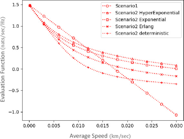
Fig. 8 shows a comparison of the evaluation function among Scenario 1 and Scenario 2, where is computed for Scenario 1, and is computed for Scenario 2 with replaced by in (25). In Fig. 8, follows four different distributions; exponential distribution, Erlang distribution, hyper-exponential distribution, and deterministic case, any of which have the same mean value . There is only one curve exhibited for because depends on only through its mean, and thus all the four cases are the same for . The horizontal axis in the figure denotes . From Fig. 8, we conclude that Scenario 1 is better when the average speed of the moving UE is sufficiently slow, whereas Scenario 2 is preferred when the UE moves fast. This is because the cost of performing an HO becomes larger as the UE moves faster, and therefore the performance of the HO skipping scenario outperforms the non-skipping scenario. Moreover, the figure shows that the distribution of the moving speed of the UE has a large impact on the evaluation function in Scenario 2 even if the average speed is the same. In particular, the evaluation function in Scenario 2 becomes larger as becomes larger in the convex order (see, e.g. [25]), that is, the expectation of the evaluation function becomes larger as the distribution of exhibits stronger randomness.
IV-B Optimizing Performance in Time-based HO Skipping Scenario
In this section, we further evaluate the transmission performance in Scenario 2 to characterize the time-based HO skipping. Our main purpose in this section is to see whether there is an optimal skipping time that maximizes the evaluation function given in (II-C) with respect to . Here, we consider a fixed moving distance in a movement period as in Section III, so that the speed of a UE in a movement period is equal to a constant . To emphasize the dependence on the moving speed , we define , which we regard as a function of . The evaluation function is expressed as
| (26) |
where (14) is applied in the second equality, and and are respectively given in (15) and (7). Although the parameter in the function above is a positive integer, we here modify the function so as to make continuous as follows; we regard the sum on the right-hand side of (26) as a Riemann sum and approximate it by the corresponding integral, that is,
| (27) |
In addition, we replace in (26) with in (21) for the sake of simplicity. Then, using , we obtain an approximate continuous function of as follows:
| (28) |
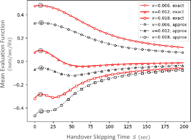
As demonstrated in Fig. 7, the approximation contains some errors. Thus, we here discuss the approximation error of compared to . Fig. 9 shows comparison results of the evaluation functions and , which are numerically computed with different and fixed , and . From the figure, we see that both the evaluation functions and have similar shapes, although there are some errors between those two functions. In particular, both and exhibit a local maximum with respect to the skipping time . In addition, both of the local optimal skipping times for and take similar values. Also, the local optimal skipping time is almost invariant with respect to exhibited in the figure. Furthermore, since and converge to zero as increases, the local maximum can be regarded as the global maximum when is sufficiently small. Therefore, the results indicate that there is an optimal skipping time that improves the evaluation function of transmission performance of a moving UE. Because both the exact and approximate evaluation functions have similar optimal skipping time, we henceforth evaluate the optimal skipping time that maximizes instead of .
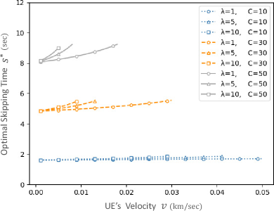
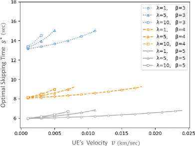
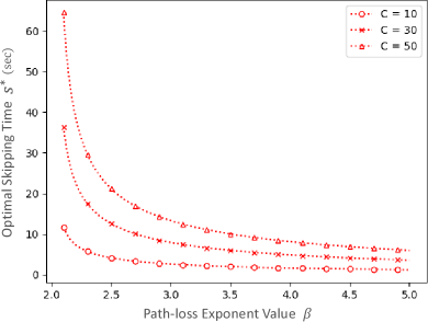
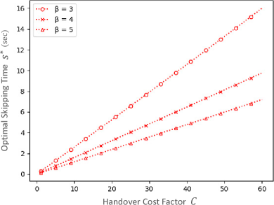
We now investigate by evaluating the impact of the other system parameters. We numerically compute and compare the results among several patterns for the values of , and . Figs. 10, 11, 12, and 13 show numerical results of the value of . The horizontal axes in these figures denote in Fig. 10, 11, in Fig. 12, and in Fig. 13, respectively, and the remaining parameters are fixed for each curve. We note that the curves are terminated when does not exist on , which occurs when any of the parameters , and exceed a certain threshold; does not exist when or is sufficiently large, or is sufficiently small. From the figures, we see that changes drastically with respect to or , whereas changes slightly with respect to or . The reason for this is that the data rate and the HO rate, the two factors constituting the evaluation function in (28), are affected by similar orders with respect to and , thus the two factors cancel each other. Moreover, from Fig. 12, we see that becomes small as increases. As we see in Fig. 6, the data rate decreases more rapidly with respect to the skipping time when is larger. Therefore, smaller provides better results when is larger. Furthermore, we see from Fig. 13 that becomes large as increases. This is intuitively because increasing makes the cost of HOs larger, and therefore longer skipping time is preferred to improve the performance. Analytical studies about these behaviors of are given in the next section.
IV-C Analytical Expressions of the Optimal Skipping Time
As shown in the numerical results in the previous section, the evaluation function in the time-based HO skipping scenario can be maximized with respect to the skipping time . An interesting feature in these results is that the skipping time that gives the maximum is almost invariant with respect to the moving speed . On the basis of this observation, we derive the theoretical expressions of the optimal skipping time approximately under the condition that the moving speed is asymptotically close to zero. Then, we apply them to the general cases of . The approximate expression of is given as follows.
Proposition 3
Proof:
To obtain the first derivative of with respect to , we consider the Taylor expansion around , and ignore terms for which the order of is greater than 2. Then, the first term of yields
| (30) |
Regarding the second term of in (28), we consider the asymptotical form of in (7) under the condition that . Since yields , in (8) is expressed as follows
where the Maclaurin expansion of is applied in the first equality, and (9) is used in the second equality. Substituting the above expression into (7) yields
where the Maclaurin expansion of the exponential form is applied in the first equality. Therefore, we have
| (31) |
From (30) and (31), we derive the asymptotical form of the first-order derivative of as
It follows from the expression above that the approximate form of the function is concave and has only one peak because is a linear function with respect to , and when is sufficiently small and when is sufficiently large. Thus, the extreme point of corresponds to the maximum with respect to .
Finally, solving for completes the proof. ∎
Remark 6
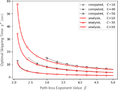
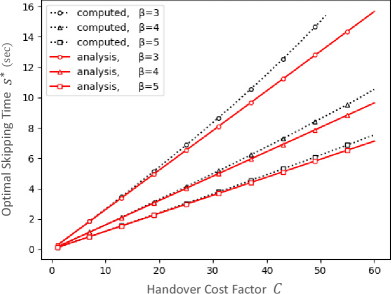
We here discuss the accuracy of the approximate expression in (29). The expression indicates that the optimal skipping time depends only on and , not on . Figs. 10 and 11 demonstrate that slightly changes with respect to even if is large. Therefore, the approximate expression (29) is expected to have sufficient accuracy in terms of the parameter when we apply (29) for general . We thus examine the accuracy of the expression in terms of and . Figs. 14 and 15 show a comparison between the approximate expression of in (29) and the exact value of obtained by numerical computation. The horizontal axes in Figs. 14 and 15 denote , and respectively. We conclude that the expression in (29) fits to the numerical result with small errors, even when is not close to zero. Thus, it appears that we can adopt (29) as an approximated result of the expression of for general , and .
Remark 7
The expression in (29) particularly implies that the optimal skipping time increases linearly as increases. This is due to the form of ; the evaluation function given in our model is an increasing linear function with respect to .
V Conclusion
In this paper, we proposed a novel HO skipping scheme, time-based HO skipping, and provided a random walk mobility model for a moving UE that performs the time-based HO skipping. Under the model of single-tier downlink cellular networks where BSs are allocated according to homogeneous PPP, we derived theoretical expressions of the two metrics: the expected data rate and the HO rate for a moving UE that performs the time-based HO skipping. On the basis of these theoretical results, we studied transmission performance of a moving UE using the two metrics, under the model of the time-based HO skipping. From our analysis, we found that the transmission performance in the time-based HO skipping scenario can outperform the non-skipping scenario when the moving speed of a UE is sufficiently large. Moreover, we found that there is a local maximum of the transmission performance with respect to the skipping time of a UE. We also investigated to derive a theoretical expression of the skipping time that gives the maximum.
For further study, our mobility model assumed that a UE moves along a straight line during a movement period, that is, a UE cannot moves along a curve in our model. Therefore, it would be expected to extend our analysis to more general trajectory model of a moving UE.
References
- [1] K. Tokuyama and N. Miyoshi, “Data rate and handoff rate analysis for user mobility in cellular networks,” IEEE WCNC 2018, pp. 1-6, 2018.
- [2] B. Romanous, N. Bitar, A. Imran, and H. Refai, “Network densification: Challenges and opportunities in enabling 5G,” 20th Int. Workshop on CAMAD, pp. 129–134, 2015.
- [3] R. Arshad, H. Elsawy, S. Sorour, T. Y. Al-Naffouri, and M.-S. Alouini, “Handover management in dense cellular networks: A stochastic geometry approach,” IEEE ICC 2016, pp. 1-7, 2016.
- [4] R. Arshad, H. Elsawy, S. Sorour, T. Y. Al-Naffouri, and M.-S. Alouini, “Velocity-aware handover management in two-tier cellular networks,” IEEE Trans. Wireless Commun., vol. 16, pp. 1851–1867, 2017.
- [5] R. Arshad, H. Elsawy, S. Sorour, T. Y. Al-Naffouri, and M. S. Alouini, “Cooperative handover management in dense cellular networks,” IEEE GLOBECOM 2016, pp. 1–6, 2016.
- [6] R. Arshad, H. Elsawy, S. Sorour, T. Y. Al-Naffouri, and M. S. Alouini, “Handover management in 5G and beyond: A topology aware skipping approach,” IEEE Access, vol. 4, pp. 9073–9081, 2016.
- [7] E. Demarchou, C. Psomas, and I. Krikidis, “Mobility management in ultra-dense networks: Handover skipping techniques,” IEEE Access, vol. 6, pp. 11921–11930, 2018.
- [8] C. Suarez-Rodriguez, Y. He, B. A. Jayawickrama and E. Dutkiewicz, “Low-Overhead Handover-Skipping Technique for 5G Networks,” IEEE WCNC 2019, pp. 1-6, 2019.
- [9] X. Wu, and H. Haas, “Handover skipping for LiFi,” IEEE Access, vol. 7, pp. 38369–38378, 2019.
- [10] M. Tayyab, X. Gelabert, R. Jantti, “A survey on handover management: From LTE to NR,” IEEE Access, vol. 7, pp. 118907–118930, 2019.
- [11] A. H. Zahran, B. Liang, and A. Saleh, “Signal threshold adaptation for vertical handover in heterogeneous wireless networks,” Mobile Netw. Appl., vol. 11, pp. 625-640, 2006.
- [12] H. Zhang, W. Ma, W. Li, W. Zheng, X. Wen, and C. Jiang, “Signalling cost evaluation of handover management schemes in LTE-advanced femtocell,” IEEE 73rd VTC, pp. 1-5, 2011.
- [13] M. Ylianttila, M. Pande, J. Makela and P. Mahonen, “Optimization scheme for mobile users performing vertical hand-offs between IEEE 802.11 and GPRS/EDGE networks,” IEEE GLOBECOM 2001, vol. 6, pp. 3439–3443, 2001.
- [14] F. Baccelli and S. Zuyev, “Stochastic geometry models of mobile communication networks,” Frontiers in Queueing, CRC Press, pp. 227–243, 1997.
- [15] X. Lin, R. K. Ganti, P. J. Fleming, and J. G. Andrews, “Towards understanding the fundamentals of mobility in cellular networks,” IEEE Trans. Wireless Commun., vol. 12, pp. 1686–1698, 2013.
- [16] J. G. Andrews, F. Baccelli, and R. K. Ganti, “A tractable approach to coverage and rate in cellular networks,” IEEE Trans. Commun., vol. 59, pp. 3122–3134, 2011.
- [17] M. Di Renzo, A. Guidotti, and G. E. Corazza, “Average rate of downlink heterogeneous cellular networks over generalized fading channels: A stochastic geometry approach,” IEEE Trans. Commun., vol. 61, pp. 3050–3071, 2013.
- [18] W. Bao and B. Liang, “Stochastic geometric analysis of user mobility in heterogeneous wireless networks,” IEEE J. Sel. Areas Commun., vol. 33, pp. 2212–2225, 2015.
- [19] W. Bao and B. Liang, “Stochastic geometric analysis of handovers in usercentric cooperative wireless networks,” IEEE INFOCOM 2016, pp. 1-9, 2016.
- [20] A. Chattopadhyay, B. Błaszczyszyn, and E. Altman, “Two-tier cellular networks for throughput maximization of static and mobile users,” IEEE Trans. Commun., vol. 18, pp. 997–1010, 2019.
- [21] S. Sadr and R. S. Adve, “Handoff rate and coverage analysis in multitier heterogeneous networks,” IEEE Trans. Commun., vol. 14, pp. 2626–2638, 2015.
- [22] S. N. Chiu, D. Stoyan, W. S. Kendall, and J. Mecke, Stochastic Geometry and its Applications, 3rd ed. Wiley, 2013.
- [23] K. A. Hamdi, “A useful lemma for capacity analysis of fading interference channels,” IEEE Trans. Commun., vol. 58, pp. 411–416, 2010.
- [24] H. Q. Nguyen, F. Baccelli, and D. Kofman, “A stochastic geometry analysis of dense IEEE 802.11 networks,” IEEE INFOCOM 2007, pp. 1199–1207, 2007.
- [25] M. Shaked, and J. G. Shanthikumar, Stochastic Orders, Springer, 2007.