Proposal for a nanomechanical qubit

Abstract

Mechanical oscillators have been demonstrated with very high quality factors over a wide range of frequencies. These also couple to a wide variety of fields and forces, making them ideal as sensors. The realization of a mechanically-based quantum bit could therefore provide an important new platform for quantum computation and sensing. Here we show that by coupling one of the flexural modes of a suspended carbon nanotube to the charge states of a double quantum dot defined in the nanotube, it is possible to induce sufficient anharmonicity in the mechanical oscillator so that the coupled system can be used as a mechanical quantum bit. This can however only be achieved when the device enters the ultrastrong coupling regime. We discuss the conditions for the anharmonicity to appear, and we show that the Hamiltonian can be mapped onto an anharmonic oscillator, allowing us to work out the energy level structure and how decoherence from the quantum dot and the mechanical oscillator are inherited by the qubit. Remarkably, the dephasing due to the quantum dot is expected to be reduced by several orders of magnitude in the coupled system. We outline qubit control, readout protocols, the realization of a CNOT gate by coupling two qubits to microwave cavity, and finally how the qubit can be used as a static force quantum sensor.

I Introduction

Mechanical systems have important applications in quantum information and quantum sensing, with for example significant recent interest in their use for frequency conversion between optical and microwave signals [1, 2, 3, 4, 5, 6], the sensing of weak forces using position detection at or beyond the standard quantum limit [7], and demonstrations of mechanically-based quantum buses and memory elements [8, 9, 10, 11, 12]. Realizing a quantum bit (qubit) based on a mechanical oscillator is thus a highly desirable goal, providing the quantum information community with a new platform for quantum information processing and storage with a number of unique features. A hallmark of mechanical resonators is their ability to couple to a variety of external perturbations, as any force leads to a mechanical displacement; a mechanical qubit could thus enable quantum sensing [13] of a wide range of force-generating fields. Another outstanding aspect is that mechanical oscillators can be designed to exhibit very large quality factors [14, 15], thus well-isolated from their environment, with correspondingly long coherence times. Mechanical devices may offer the possibility to develop quantum circuits with both a large number of qubits and a long qubit decoherence time. This is of considerable relevance to quantum computing, since the decoherence times of superconducting qubits integrated in large scale circuits [16] are reduced to of order 10 $\mu s$, which is much lower than what can be achieved when operating single superconducting qubits [17].

A mechanical oscillator can be made into a qubit by introducing a controlled anharmonicity, thereby introducing energy-dependent spacing in the oscillator’s quantized energy spectrum [18, 19]. The anharmonicity then enables the controlled and selective excitation of energy states of the system, for example the ground and first excited state, without populating other states, breaking the strong correspondence principle that otherwise limits the quantum control of harmonic systems.

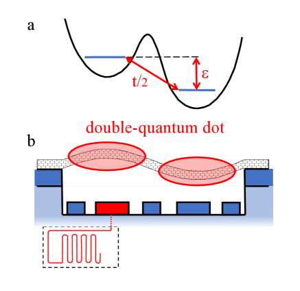
Figure 1: Schematic of the proposed setup. A suspended carbon nanotube hosting a double quantum dot, whose one-electron charged state is coupled to the second flexural mode. (a) Sketch of the electronic confinement potential and of the two main parameters, the hopping amplitude $t$ and the energy difference $\epsilon$ between the two single-charge states. (b) Physical realization. One of the gate electrodes is connected to a microwave cavity for dispersive qubit readout.

Notwithstanding the apparent simplicity of this idea, finding mechanical oscillators with sufficiently strong and controllable anharmonicity is not trivial. In Ref. 18, 19, anharmonicity induced by proximity to a buckling instability has been proposed. However, such a scheme is difficult to achieve experimentally. Here we consider the possibility of coupling one of the flexural modes of a carbon nanotube to an integrated double quantum dot, the dot itself defined in the nanotube (cf. Fig. 1). By tuning independently the gate voltages for the two quantum dots, it is possible to select the low-energy electronic states so that only those with a single (additional) electron on the double quantum dot are energetically accessible. The excess electron can sit either on the left or the right dot. This charged two-level system is electrostatically coupled to the displacement of the oscillator, in particular to the second flexural mode, as illustrated in Fig. 1.

We show in the following that for sufficiently strong electro-mechanical coupling, the double quantum dot induces a bistability in the mechanical mode, by reducing and then changing the sign of the quadratic term of the effective mechanical potential. We find that for strong, but nonetheless reachable coupling constants, it is possible in this way to generate an anharmonicity sufficient to transform the mechanical oscillator into a qubit; this does however require entering the so-called ultrastrong coupling regime, where the coupling strength is larger than the mechanical energy level spacing.

Remarkably, we also find that in the dispersive limit of large detuning of the oscillator frequency and the electronic two-level system energy splitting, the problem can be mapped onto the Hamiltonian of the quantum-anharmonic oscillator, allowing use of results from that system in this work. Following a description of the anharmonically-coupled system, we investigate the decoherence induced by the charged two-level system on the mechanical qubit, as well as how standard protocols for quantum manipulation can be implemented. The reduction of the pure-dephasing rate of the mechanical qubit with respect to that of the charged two-level system can be made larger than $10^{3}$ with parameters accessible experimentally. We show how qubit readout and manipulation can be achieved as well as how a CNOT gate for two nanomechanical qubits could be realized by coupling them to the same microwave cavity. We also show that the mechanical qubit can be used as a quantum sensor for any static force that could displace the oscillator. The static force sensitivity can reach values as good as $10^{-21}{\rm N}/{\rm Hz}^{1/2}$.

II Model

We consider a nanomechanical system [20, 21, 22, 23, 24, 25, 26, 27] based on a suspended carbon nanotube (cf. Fig. 1) similar to those demonstrated by a number of groups [28, 29, 30, 31]. It has been shown that it is possible to use multiples gates to fine-tune the electrostatic potential along the suspended part of the nanotube [32, 33, 29]. It is thus possible to form a double-well potential to engineer a double quantum dot. We consider the case when only two states, each with one excess electron, are energetically accessible [34], the other states being at higher energy due to the Coulomb interaction. The two single-charge states, corresponding to an electron on the left or right dot, are coupled by a hopping term $t/2$. Their relative energy difference, $\epsilon$, can be controlled by varying the two gate voltages. The two states couple to the nanotube flexural modes. By placing the double dot in the center of the nanotube, the coupling of the two charge states with the second (anti-symmetric) mechanical mode is maximized (cf. Fig. 1).

A model Hamiltonian capturing the basic physics of this system can be written down:

$$H={p^{2}\over 2m}+\frac{m\omega_{\rm m}^{2}x^{2}}{2}+\frac{\epsilon}{2}\sigma_{z}+\frac{t}{2}\sigma_{x}-\hbar g\frac{x}{{x_{\rm z}}}\sigma_{z}\,,$$ (1)

where the first two terms describe the relevant mechanical mode of frequency $\omega_{\rm m}/2\pi$ with effective mass $m$, displacement $x$, momentum $p$, and we have introduced the zero-point quantum fluctuation ${x_{\rm z}}=(\hbar/2m\omega_{\rm m})^{1/2}$ with $\hbar$ the reduced Planck constant. The electronic response has been reduced to a two-level system, where the two Pauli matrices $\sigma_{z}$ and $\sigma_{x}$ represent the dot charge energy splitting and inter-dot charge hopping, respectively. Finally $\hbar g/{x_{\rm z}}$ is the variation of the force acting on the mechanical mode when the charge switches from one dot to the other. The value and sign of $g$ can be tuned over a large range by adjusting the gate voltages [14]. In Appendix A we give a microscopic derivation of the Hamiltonian with the explicit form of the coupling terms.

III Born-Oppenheimer picture

To gain an insight into the physics of the problem, it is instructive to first consider a semi-classical Born-Oppenheimer picture valid for $\hbar\omega_{\rm m}\ll\sqrt{t^{2}+\epsilon^{2}}$. We diagonalize $H$ given by Eq. (1), neglecting the $p^{2}$ term and regarding $x$ as a classical variable. The two eigenvalues read:

$$\varepsilon_{\pm}(x)={m\omega_{\rm m}^{2}x^{2}/2}\pm\sqrt{(\epsilon-2\hbar gx/{x_{\rm z}})^{2}+t^{2}}/2.$$ (2)

In the spirit of Born-Oppenheimer approximation, the energy profile $\varepsilon_{\pm}$ can be regarded as an effective potential for the oscillator, which depends on which charge quantum level is occupied. Taylor-expanding $\varepsilon_{\pm}(x)$ for small $x$ and $\epsilon=0$ one finds:

$$\varepsilon_{\pm}=\pm{t\over 2}+{m\omega_{\rm m}^{2}\over 2}\left(1\pm{4\hbar g^{2}\over\omega_{\rm m}t}\right)x^{2}\mp{4m^{2}\omega_{\rm m}^{2}\hbar^{2}g^{4}\over t^{3}}x^{4}+\dots\,.$$ (3)

The coupling to the double dot leads to a renormalization of the quadratic coefficient and the appearance of a quartic and higher terms. The interaction stiffens the resonating frequency of the upper branch while softening the lower one. In particular, for $g>g^{\rm sc}_{c}=(\omega_{\rm m}t/4\hbar)^{1/2}$, the quadratic coefficient of the lower branch becomes negative. This leads to a double-well potential and a bistability similar to that predicted for a single quantum dot coupled to a mechanical oscillator [35, 25, 27, 36, 37].

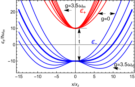
Figure 2: Effective potentials $\varepsilon_{+}(x)$ (red) and $\varepsilon_{-}(x)$ (blue) from Eq. (2) for $t/\hbar\omega_{\rm m}=20$ and the values of $(4g/\omega_{\rm m})^{2}=0$, 10, 20, 30, 40, 50, with the first and last line explicitly indicated in the figure. The potential for $g=g_{c}^{\rm sc}=\omega_{\rm m}\sqrt{5}$ is shown with a thicker line.

Figure 2 shows the evolution of the two branches of the potential as a function of the coupling constant $g$, for an experimentally-accessible value of $t=20\hbar\omega_{\rm m}$. One clearly sees the formation of the double well-potential for $g>g^{\rm sc}_{c}$. For $g=g^{\rm sc}_{c}$ the potential of the lower branch is purely quartic (thick line). Thus one expects that tuning $g$ close to this critical value, it should be possible to modify, over a large range, the ratio between the quadratic and quartic terms and consequently tune the degree of anharmonicity of the system at will.

IV Full Quantum description

IV.1 Conditions for anharmonicity

The validity of the qualitative description of the previous section can be confirmed in the general case by numerical diagonalization of the Hamiltonian given by Eq. (1) in a truncated Hilbert space. Using a basis comprising the $10^{2}$ lowest harmonic oscillator states largely suffices to reach convergence and we find the Hamiltonian eigenvectors $|n\rangle$ and eigenstates $E_{n}$ for the problem. The result for the lowest set of energy levels is shown in Fig. 3.

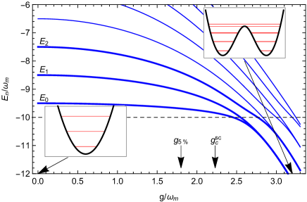
Figure 3: Lowest-lying energy eigenvalues $E_{n}$ of the Hamiltonian (1) for $\epsilon=0$ and $t=20\hbar\omega_{\rm m}$ as a function of $g/\omega_{\rm m}$. The Born-Oppenheimer potential given by Eq. (2) and the energy levels are shown in the insets for $g=0$ and $g=3.2\omega_{\rm m}$. The dashed line indicates the lowest non-interacting electronic level $-t/2$. The semiclassical critical value for the bistability is $g^{\rm sc}_{c}/\omega_{\rm m}=\sqrt{5}\approx 2.23$. The value of $g=g_{5\%}\approx 1.8\omega_{\rm m}$ for which the anharmonicity is $5\%$ is also shown.

We first notice that for $g\sim g_{\rm c}^{\rm sc}$, the ground state crosses the lowest non-interacting electronic level, indicated by the dashed line $-t/2$, preceding the formation of two bound states in the double-well. Note that one expects that this crossing should occur for a coupling larger than $g_{\rm c}^{\rm sc}$, since for this value the problem reduces to a quartic oscillator, for which the ground state has a positive value [38] similarly to the harmonic oscillator zero-point motion $\hbar\omega_{\rm m}/2$. For $g\gg g_{\rm c}^{\rm sc}$, the above mentioned bound states have the same energy (cf. the upper-right inset in Fig. 3) and are sufficiently far from each other that their overlap is negligible. In Fig. 3, the third level remains well separated from the first two, and merges with the fourth level for large $g$. We introduce the transition frequencies $\omega_{nm}=(E_{n}-E_{m})/\hbar$. The anharmonicity, defined as

$$a={\omega_{21}-\omega_{10}\over\omega_{10}}\,,$$ (4)

thus diverges as we increase $g$ from 0 to a value of the order of $g_{\rm c}^{\rm sc}$. As discussed in the introduction, this anharmonicity is crucial to enabling quantum control of the qubit formed by the first two levels, $|0\rangle$ and $|1\rangle$. A minimum requirement is that the transition frequency $\omega_{10}$ between $|0\rangle$ and $|1\rangle$ needs to differ from $\omega_{12}$ between $|1\rangle$ and $|2\rangle$ by much more than the spectral linewidth of the states. As a practical example, in the superconducting transmon qubit [39], an anharmonicity of the order of 5% suffices to afford full quantum control of the qubit states. In the following we will thus consider 5% anharmonicity as a (somewhat arbitrary) requirement; this is sufficient to find the relevant coupling scale required to implement the mechanical qubit.

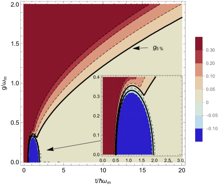
Figure 4: Contour plot of the anharmonicity $a$ in the $(t,g)$ plane. The contour line for $a=0.05$ is thicker, and defines the function $g_{5\%}(t)$. The kink at $t\approx 1.54\hbar\omega_{\rm m}$ of this function, better seen in the inset, is due to the avoided crossing between the charge and oscillator eigenstates that occurs at that value of $t$. It indicates the region where the eigenstate begins to have a predominantly charge nature.

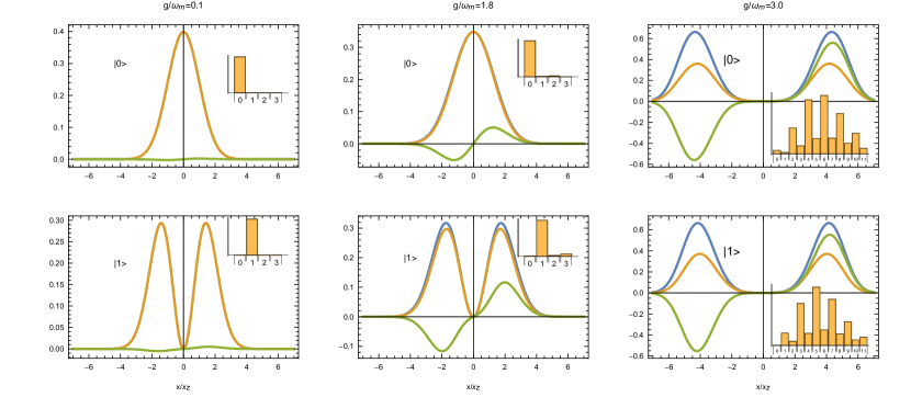
Figure 5: Wavefunctions of the two qubit states $|0\rangle$ (upper panels) and $|1\rangle$ (lower panels) for $t/\hbar\omega_{\rm m}=20$, $g/\omega_{\rm m}=0.1$, 1.8, and 3.0. We plot -$\langle\sigma_{x}\rangle(x)$ (yellow), $\langle\sigma_{z}\rangle(x)$ (green), and $\psi_{n+}(x)^{2}+\psi_{n-}(x)^{2}$ (blue). Note that for small coupling the yellow and blue lines perfectly overlap. The probability of occupation of the first single-harmonic oscillator states are indicated in the insets.

Resorting again to numerical diagonalization, we present in Fig. 4 a contour plot for the dependence of the anharmonicity on the parameters $t$ and $g$. The thick contour line for $a=0.05$ defines the function $g_{5\%}$, which gives the required coupling to obtain a 5% anharmonicity. The region for $t<2\hbar\omega_{\rm m}$ presents a more complex structure. A weaker coupling is required to reach the needed anharmonicity. But in this region the first two levels inherit the properties of the double quantum dot to a large extend, so that we will not discuss it further. Here we explore the mechanical qubit in the parameter range when $t>2\hbar\omega_{\rm m}$, so that the nature of the two lowest energy states of the coupled system remains mechanical. A sizable anharmonicity can only be reached when operating the device near or in the ultra-strong coupling regime, $g>\omega_{\rm m}$, as seen in Fig. 4.

IV.2 Eigenstates

It is interesting to investigate the nature of the two qubit states $|0\rangle$ and $|1\rangle$. In the position representation, the wavefunction is given by $\psi_{n\sigma}(x)=\langle x,\sigma|n\rangle$, where $|n\rangle$ the Hamiltonian eigenstate and $|x,\sigma\rangle$ is the eigenstate of the displacement $x$ and $\sigma_{z}$ operators with eigenvalues $x$ and $\sigma$, respectively. The wavefunction $\psi_{n\sigma}(x)$ can be chosen to be real-valued. Instead of looking directly at $\psi_{n\sigma}(x)$, it is more interesting to consider the averages of the operators $\sigma_{i}$ as a function of $x$: $\langle\sigma_{i}\rangle(x)=\sum_{\sigma,\sigma^{\prime}}\psi_{n\sigma}(x)[\sigma_{i}]_{\sigma\sigma^{\prime}}\psi_{n\sigma^{\prime}}(x)$. Since by symmetry $\langle\sigma_{y}\rangle=0$, only $\langle\sigma_{x}\rangle=2\psi_{n+}\psi_{n-}$ and $\langle\sigma_{z}\rangle=\psi_{n+}^{2}-\psi_{n-}^{2}$ are non-vanishing.

We display in Fig. 5 these two components as well as the total probability for the oscillator displacement $\psi^{2}=\psi_{n+}^{2}+\psi_{n-}^{2}$ (blue curve in Fig. 5). The function $\langle\sigma_{z}\rangle(x)$ gives the distribution of the charge (green curve in Fig. 5), while $\langle\sigma_{x}\rangle(x)$ indicates the strength of the coherent superposition of the two charge-states (yellow curve in Fig. 5). These two quantities are in competition. From the figure, one sees that for weak coupling $\langle\sigma_{z}\rangle(x)\approx 0$, and the displacement probability distribution coincides with $-\langle\sigma_{x}\rangle(x)$. At the value of $g=g_{5\%}$, the distribution of the charge depends on $x$, for both states. Finally for the bistable case with $g/\omega_{\rm m}=3.0$, one reaches the limit where $|\langle\sigma_{z}\rangle(x)|$ is close to the displacement probability, indicating a full correlation between the displacement and the charge. We also show in the figure the distribution of the harmonic oscillator states. One clearly sees that for $g=g_{5\%}$, the two states are still mainly eigenstates of the mechanical oscillator.

IV.3 Mapping in the dispersive regime

The numerical diagonalization shows that the semiclassical picture provides a good qualitative description. A natural question is then how far one can extend this picture. For this reason, we looked for a unitary transformation $U$ that could map the Hamiltonian given in Eq. (1) onto that of a simple anharmonic oscillator. In the limit of $g/|t/\hbar-\omega_{\rm m}|\ll 1$, known as the dispersive limit, we find a $U$ such that, at fourth order in $g$, we can write $H_{T}=U^{\dagger}HU$ with

$$H_{T}={t\over 2}\sigma_{z}+{\hbar\omega_{\rm m}\over 4}\left[\alpha_{1}{\hat{p}}^{2}+\alpha_{2}{\hat{x}}^{2}+\sigma_{z}(\alpha_{3}{\hat{x}}^{2}+\alpha_{4}{\hat{x}}^{4})\right]\,.$$ (5)

[We discarded the constant $\hbar^{3}g^{2}\omega_{\rm m}/(t^{2}-\hbar^{2}\omega_{\rm m}^{2})$.] Here we introduce the quadratures $\hat{x}=x/{x_{\rm z}}=a^{\dagger}+a$, $\hat{p}=p/(m\omega_{\rm m}{x_{\rm z}})=i(a^{\dagger}-a)$, with $[{\hat{x}},{\hat{p}}]=2i$, where $a$ and $a^{\dagger}$ are the creation and destruction operators for the harmonic oscillator eigenstates. The four coefficients read

$$\alpha_{1} = 1+{128\hbar^{6}g^{4}t^{2}\omega_{\rm m}^{2}\over\Delta^{6}\Delta_{3}^{2}},\qquad\alpha_{2}=1-{16\hbar^{4}g^{4}t^{2}\over\Delta^{4}\Delta_{3}^{2}},$$ (6)

$$\alpha_{3} = {4\hbar tg^{2}\over\omega_{\rm m}\Delta^{2}},\qquad\alpha_{4}=-{4\hbar^{3}tg^{4}(3t^{2}+\hbar^{2}\omega_{\rm m}^{2})\over 3\omega_{\rm m}\Delta^{6}}\,,$$ (7)

where $\Delta^{2}=t^{2}-(\hbar\omega_{\rm m})^{2}$, $\Delta_{3}^{2}=t^{2}-9(\hbar\omega_{\rm m})^{2}$. The derivation and the definition of $U$ are given in Appendix B.

Remarkably we find that within this approximation, it is possible to map the problem onto a new description with two anharmonic oscillators, one for each charge branch. The upper branch is unstable if we stop the expansion at $x^{4}$, since it has a negative quartic term. This description thus holds for a small but non-zero value of the ratio $\hbar\omega_{\rm m}/t$, giving a more accurate description than the simpler Born-Oppenheimer approach.

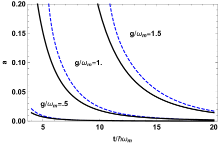
Figure 6: Comparison between numerical (full line) and analytical (dashed line) dependence of the anharmonicity parameter $a$ for three values of the coupling $g/\omega_{\rm m}$=0.5, 1, 1.5.

The anharmonic oscillator is a well-studied problem [40]. When the quadratic part is positive, it is convenient to write the lower branch of Eq. (5) in the standard form,

$$H=\hbar\omega_{\rm m}^{\prime}({\hat{x}}^{2}+{\hat{p}}^{2}+\lambda{\hat{x}}^{4})/4.$$ (8)

This can be done by the scaling ${\hat{x}}=\xi{\hat{x}}^{\prime}$ and ${\hat{p}}={\hat{p}}^{\prime}/\xi$, so that the commutation relation is preserved $[{\hat{x}}^{\prime},{\hat{p}}^{\prime}]=2i$, with

$$\xi=[\alpha_{1}/(\alpha_{2}-\alpha_{3})]^{1/4}\,.$$ (9)

The renormalized resonant frequency reads $\omega_{\rm m}^{\prime}=\omega_{\rm m}[\alpha_{1}(\alpha_{2}-\alpha_{3})]^{1/2}$ and the quartic coefficient is

$$\lambda={\alpha_{4}\alpha_{1}^{1/2}\over(\alpha_{2}-\alpha_{3})^{3/2}}.$$ (10)

Note that we now consider only positive values of $\omega_{\rm m}^{\prime}$, but Eq. (5) holds also in the bistable region. The anharmonicity $a$ defined in Eq. (4) becomes a function of $\lambda$ only. Using the expression (1.17) of Ref. 40 for the eigenvalues in terms of $\lambda$ and Eq. (10), one can obtain an analytical expression for the anharmonicity in terms of the parameters $\omega_{\rm m}$, $t$, and $g$ that agrees with the numerics with a reasonable accuracy, as can be seen in Fig. 6. One finds that the 5% anharmonicity is achieved for $\lambda_{c}\approx 0.0225$ (the exact numerical result is $\lambda_{c}=0.0220$).

IV.4 Operators acting on the qubit

In order to study the control, readout, and decoherence of the qubit formed by the two states $|0\rangle$ and $|1\rangle$, it is necessary to find the projection of the physical operators $\sigma_{i}$, ${\hat{x}}$, and ${\hat{p}}$ in the Hilbert space spanned by $\{|0\rangle,|1\rangle\}$. In this space, any operator can be written as a linear combination of the unit matrix ($\tau_{0}$) and the three Pauli matrices, that we define here as $\{\tau_{x},\tau_{y},\tau_{z}\}$, to distinguish them from the operators $\sigma_{i}$ acting in the charge space. The Hamiltonian of the qubit then simply reads $\hbar\omega_{10}\tau_{z}/2$. One can calculate numerically the matrix elements of any operator in the qubit sub-space and then obtain its form in terms of a sum of the four $\tau$-matrices. We find for the charge variables [in the representation of Eq. (1)]

$$\left\{\begin{array}[]{rcl}\left.\sigma_{x}\right|_{\rm qb}&=&\beta_{1}\tau_{0}+\beta_{2}\tau_{z},\\ \left.\sigma_{y}\right|_{\rm qb}&=&\beta_{3}\tau_{y},\\ \left.\sigma_{z}\right|_{\rm qb}&=&\beta_{4}\tau_{x},\end{array}\right.$$ (11)

and for the oscillator variables

$$\left\{\begin{array}[]{rcl}\left.{\hat{x}}\right|_{\rm qb}&=&\beta_{5}\tau_{x}\,,\\ \left.{\hat{p}}\right|_{\rm qb}&=&\beta_{6}\tau_{y}.\end{array}\right.$$ (12)

The six coefficients can be obtained numerically, but it is also interesting to obtain approximate analytical expressions for them. This can be achieved using the unitary transformation introduced above (see Appendix B):

$$\beta_{1} = -1+4(\hbar g)^{2}{(\hbar\omega_{\rm m})^{2}-t\hbar\omega_{\rm m}\xi^{2}+t^{2}\xi^{4}\over\Delta^{4}\xi^{2}}+g^{4}\beta_{1,4}\,,$$

$$\beta_{2} = -2(\hbar g)^{2}{(\hbar\omega_{\rm m})^{2}+t^{2}\xi^{4}\over\Delta^{4}\xi^{2}}+g^{4}\beta_{2,4}\,,$$ (14)

$$\beta_{3} = {2\hbar^{2}g\omega_{\rm m}\over\Delta^{2}\xi}+g^{3}\beta_{3,3}\,,$$ (15)

$$\beta_{4} = {2\hbar gt\xi\over\Delta^{2}}+g^{3}\beta_{4,3}\,,$$ (16)

$$\beta_{5} = \xi-{2\hbar^{3}g^{2}t\omega_{\rm m}\xi\over\Delta^{4}}+g^{4}\beta_{5,4}\,,$$ (17)

$$\beta_{6} = {1\over\xi}-{2\hbar^{3}g^{2}t\omega_{\rm m}\over\Delta^{2}\xi}+g^{4}\beta_{6,4}.$$ (18)

The coefficients for $g^{3}$ and $g^{4}$ are given by Eqs. (91)-(96) in the Appendix.

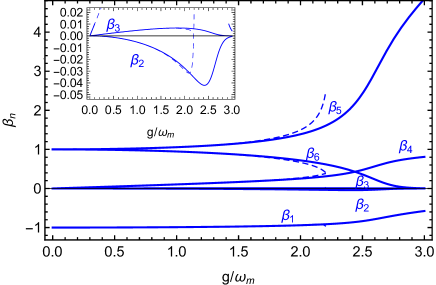
Figure 7: Coefficients $\beta_{i}$ of the operator projections in the qubit space, obtained by numerical diagonalization (full lines) and from the analytical approximation to fourth order in $g$ (dashed lines). The value of $t$ is fixed here to $20\hbar\omega_{\rm m}$.

We show in Fig. 7 the behavior of the analytic coefficients as a function of $g/\omega_{\rm m}$ for $t/\hbar\omega_{\rm m}=20$, and compare to the exact numerical results. The analytical expressions again give a good description in the interesting range $g<g_{5\%}$. In particular, these expressions allow us to recognize that $\beta_{2}$ and $\beta_{3}$ are parametrically small for $g\approx\omega_{m}\ll t/\hbar$.

Another important result given by the expressions for the $\beta_{i}$ is the charge component of the qubit. This can be identified with the value of the $\beta_{4}$ coefficient, which gives the projection of the charge operator $\sigma_{z}$ in the qubit space. This coefficient vanishes linearly in $g$, and it remains small up to $g\approx\sqrt{\omega_{\rm m}t/\hbar}$ when $t\gg\hbar\omega_{\rm m}$. In this case, we thus expect that the qubit has a predominantly mechanical character in its degrees of freedom, measured by the $\beta_{5}$ and $\beta_{6}$ coefficients, which remain of the order of unity.

IV.5 Qubit Manipulation

The values of $\beta$ are also crucial to understanding how to manipulate the qubit. This is achieved using a completely classical oscillating voltage applied to a nearby wire, turned on for some duration with a calibrated amplitude. The anharmonicity of the system allows this classical signal to achieve quantum control. One can find the effect of an oscillating voltage on the qubit by considering how this voltage couples to the $\sigma_{i}$ and ${\hat{x}}$ operators. In Appendix A, we derive these couplings for a potential $V_{g12}^{\rm AC}$ applied to the two gates controlling the electrochemical potential of each dot [cf. Eq. (75)]. We find that the potential couples to $\sigma_{z}$ and ${\hat{x}}$ with the coefficients $\lambda^{\rm ev}$ and $\lambda^{\rm mv}{x_{\rm z}}$, respectively (see Appendix A for the explicit expressions). Since both ${\hat{x}}$ and $\sigma_{z}$ project on $\tau_{x}$, we find that the coupling to the oscillating field is just $\lambda_{v}\tau_{x}V_{g12}^{\rm AC}$ with

$$\lambda_{v}=\lambda^{\rm mv}{x_{\rm z}}\beta_{5}+\lambda^{\rm ev}\beta_{4}\,.$$ (19)

This indicates that one can use standard methods to manipulate the qubit state, e.g. by using nuclear magnetic resonance methods by driving the qubit states at a frequency $\omega_{D}$ with pulses that induce, in the rotating frame, a term $\hbar(\omega_{10}-\omega_{D})\tau_{z}/2+\lambda_{v}V_{g12}^{0}\tau_{x}$ [41]. The anharmonicity guarantees that the second excited state will not be populated by these manipulations.

IV.6 Qubit Readout

Reading out the state of the qubit can be realised by coupling the system to a microwave superconducting cavity and using a dispersive interaction, analogous to what is done with superconducting qubits [42, 43]. The coupling can be obtained from the expression of the coupling to an oscillating voltage [cf. Eqs. (73) and (74)] with the substitution $V^{\rm AC}\rightarrow V_{\rm z}(b+b^{\dagger})$, where $b$ is the destruction operator of the photons in the cavity and $V_{\rm z}$ is the zero-point voltage of the cavity. The coupling Hamiltonian reads

$$H^{\rm qb-cav}=\hbar g_{v}\tau_{x}(b+b^{\dagger})$$ (20)

with $\hbar g_{v}=\lambda_{v}V_{\rm z}$ [cf. Eq. (19)]. A standard method is then to perform a dispersive measurement of the superconducting cavity frequency, modified by an amount which depends on the qubit state. By performing a unitary transformation [44] one can eliminate the term $\tau_{x}$ from the Hamiltonian and obtain for the qubit and cavity Hamiltonian

$$H/\hbar=\omega_{10}\tau_{z}/2+(\omega_{c}+\chi\tau_{z})b^{\dagger}b$$ (21)

where $\omega_{c}$ is the cavity resonant frequency and $\chi=g_{v}^{2}/(\omega_{10}-\omega_{c})$ the dispersive frequency shift. Since the resonating frequency depends now on the qubit state, this allows us to perform an efficient quantum non-destructive readout of the qubit state.

This picture remains qualitatively correct, but in analogy with what happens in the transmon qubit [45], when the anharmonicity is small, one needs to include the other system states to calculate the dispersive coupling correctly. We present in appendix C the calculation of $\chi$ for the problem at hand by using second order perturbation theory in the coupling constant to the cavity. In this picture the eigenstates can be labeled according to the branch ($\sigma=\pm$) in Fig. 2 with $|n\sigma\rangle$ and eigenstate energy $E_{n\sigma}$. We find that the second excited state, $|2\rangle=|2-\rangle$, and two other excited states of the upper branch ($|0+\rangle$ and $|1+\rangle$) with an excitation energy of the order of $t$ contribute. The parameter $\chi$ entering Eq. (21) reads $\chi=\chi_{\rm m}+\chi_{\rm e}$, with

$$\chi_{\rm m}(\omega_{c})\approx{(g_{\rm ec}\beta_{4,1})^{2}(\omega_{21}-\omega_{10})\over(\omega_{c}-\omega_{21})(\omega_{c}-\omega_{10})}$$ (22)

dominant for $\omega_{c}\approx\omega_{10}$ and

$$\chi_{\rm e}(\omega_{c})\approx{g_{\rm ec}^{2}(\delta_{11}-\delta_{00})\over 2(\omega_{c}-\delta_{11})(\omega_{c}-\delta_{00})},$$ (23)

for $\omega_{c}\approx\delta_{00}$. Here $\beta_{4,1}=2\hbar g\xi t/\Delta^{2}\ll 1$ is the first order contribution to $\beta_{4}$ [cfr Eq. (16)], $\delta_{nm}=(E_{n+}-E_{m-})/\hbar$, and $\hbar g_{\rm ec}=\lambda^{\rm ev}V_{z}$. One can see that $\chi_{\rm m}$ is proportional to the anharmonicity, and thus vanishes in the harmonic case. The expression for $\chi_{\rm e}$ also vanishes when the coupling constant vanishes, but it does not require an anharmonicity:

$$\delta_{11}-\delta_{00}\approx{4g^{2}t\over\Delta^{2}}.$$ (24)

At lowest order this value is just the difference of the semiclassical resonating frequencies of the upper and lower branch. This dispersive coupling relies on the intrinsic anharmonicity of the charge two-level system.

We can further simplify Eq. (22) by considering it for $\omega_{c}$ close to $\omega_{10}$: the small numerator is compensated by a vanishing denominator and one obtains $\chi_{\rm m}\approx(g_{\rm ec}\beta_{4,1})^{2}/(\omega_{10}-\omega_{c})$, which remarkably coincides with the standard form of the dispersive coupling. Even if this looks independent of the anharmonicity, note that it is necessary that $|\omega_{21}-\omega_{10}|>g_{\rm ec}\beta_{4,1}$ for the calculation to be valid, this condition sets the constraint on the anharmonicity $a>g_{\rm ec}\beta_{4,1}/\omega_{10}$. Choosing the detuning to the minimum value allowed by second-order perturbation theory: $g_{\rm ec}\beta_{4,1}$, one obtains $\chi_{\rm m}^{\rm max}\approx g_{\rm ec}\beta_{4,1}<a\omega_{10}$. Since $\omega_{c}\approx\omega_{10}$ this shows that a quality factor larger than $1/a$ would be largely sufficient to detect the qubit state.

Similar arguments can be applied to the expression for $\chi_{\rm e}$, leading to $\chi_{\rm e}^{\rm max}\approx g_{\rm ec}$. In this case the limitation is less severe, since the condition $|\delta_{11}-\delta_{00}|>g_{\rm ec}$ does not involve the anharmonicity. Using Eq. (24) it gives approximately $g_{\rm ec}<4g^{2}/t$. This result suggests that it may be more convenient to tune the cavity to this resonance and exploit the $\chi_{\rm e}$ dispersive coupling to readout the qubit state.

These analytical expressions are obtained as a perturbative expansion in $g/t$, but the expressions remain accurate in the range of coupling of interest for our purposes as shown as an example in Fig. 8.

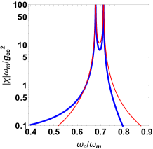
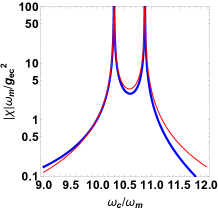
Figure 8: The quantity $|\chi|\omega_{m}/g_{\rm ec}^{2}$ for $t/\hbar\omega_{\rm m}=10$, $g/\omega_{\rm m}=1.2164$ (for which $a=0.05$) as a function of $\omega_{c}/\omega_{\rm m}$ in two different regions of the spectrum: close to $\omega_{10}<\omega_{12}$ and close to $\delta_{00}<\delta_{11}$, left and right panel, respectively. The thick blue line gives the numerical calculation, the thin red line the expressions (22) and (23), shown in the left and right panel, respectively.

V Decoherence

The double quantum dot and the mechanical oscillator are unavoidably coupled to the environment, which induces decoherence and incoherent transitions between energy levels. The decoherence rate of the double quantum dot charge qubit is much larger than that of the mechanical resonator, so that it will limit the performances of the mechanical qubit. Best values for the decoherence rate are in the MHz range [46].

In order to study how the nano-mechanical qubit inherits the decoherence of its two sub-system components, we begin by constructing a simple model for the coupling of the sub-systems to the environment.

We write the coupling Hamiltonian as

$$H_{I}={\hat{A}}^{\rm c}\hat{E}_{1}+{\hat{x}}\hat{E}_{2}\,,$$ (25)

where ${\hat{A}}^{\rm c}=\sum_{i=x,y,z}v_{i}\sigma_{i}=\vec{v}\cdot\vec{\sigma}$ is the most general operator in the charge subspace (see for instance [47]). The operators $\hat{E}_{1}$ and $\hat{E}_{2}$ are given by the sum of operators, themselves involving many degrees of freedom that model the environment of the charge and the mechanical oscillator, respectively (the coupling constant is absorbed in the $\hat{E}$-operators so that ${\hat{A}}^{\rm c}$ and ${\hat{x}}$ are dimensionless). We assume that we know the correlation functions $C_{i}(t)=\langle\hat{E}_{i}(t)\hat{E}_{i}(0)\rangle$, as well as their Fourier transforms $S_{i}(\omega)=\int dte^{i\omega t}C_{i}(t)$, and that the charge and mechanical environments are independent, $\langle\hat{E}_{1}(t)\hat{E}_{2}(0)\rangle=0$. If $S_{i}(\omega)$ is a sufficiently smooth function for $\omega$ close to the qubit resonant frequency, the three parameters $v_{i}$ give a complete description of the coupling to the environment of the charge system. For the mechanical oscillator, we parametrize the coupling to the environment with a single damping rate $\gamma$.

One can then use the standard procedure, integrating out the environmental degrees of freedom and finding an equation for the reduced density matrix $\rho$ in the Born-Markov and rotating-wave approximations. The rate equations have the standard form:

$$\dot{\rho}_{nn} = -\rho_{nn}\sum_{p\neq n}\Gamma_{n\rightarrow p}+\sum_{p\neq n}\rho_{pp}\Gamma_{p\rightarrow n},$$ (26)

$$\dot{\rho}_{nm} = -\left[\sum_{p\neq n}\Gamma_{n\rightarrow p}/2+\sum_{p\neq m}\Gamma_{m\rightarrow p}/2+\Gamma^{\phi}_{nm}\right]\rho_{nm},$$

where $\rho_{nm}=\langle n|\rho|m\rangle$ is the matrix element of $\rho$ in the eigenstate basis $|n\rangle$ of the Hamiltonian (1) with eigenvalues $E_{n}$. The rates read:

$$\Gamma_{n\rightarrow m} = 2\pi S_{1}(\omega_{nm})|A^{\rm c}_{nm}|^{2}+2\pi S_{2}(\omega_{nm})|x_{nm}|^{2},$$

$$\Gamma^{\phi}_{nm} = \pi S_{1}(0)(A^{\rm c}_{nn}-A^{\rm c}_{mm})^{2}+\pi S_{2}(0)(x_{nn}-x_{mm})^{2}$$

where $O_{nm}=\langle n|O|m\rangle$ and $\Gamma^{\phi}_{nm}$ is the pure dephasing rate. These equations hold at non-zero temperature $T$, with $S_{i}(\omega)=S_{i}(-\omega)e^{\hbar\omega/k_{B}T}$ and $k_{B}$ is the Boltzmann constant. When only two levels are present one finds

$$\dot{\rho}_{00} = -\rho_{00}\Gamma_{0\rightarrow 1}+\rho_{11}\Gamma_{1\rightarrow 0}$$ (28)

$$\dot{\rho}_{01} = -\rho_{01}(\Gamma_{0\rightarrow 1}+\Gamma_{1\rightarrow 0}+2\Gamma^{\phi}_{01})/2\,.$$ (29)

The last equation defines the coherence time of the qubit $T_{2}=2/(\Gamma_{0\rightarrow 1}+\Gamma_{1\rightarrow 0}+2\Gamma^{\phi}_{01})$. In the following we focus on the two rates $\Gamma_{1\rightarrow 0}$ and $\Gamma^{\phi}_{01}$. (We do not consider the case of equally-spaced levels inducing transfer of coherence between higher energy states [48].)

V.1 Non-interacting case

Let us begin with the non-interacting case ($g=0$) in order to define the rates. We have two independent systems: the double quantum dot and the mechanical oscillator. For the oscillator, one finds $\Gamma^{\rm m}_{1\rightarrow 0}=2\pi S_{2}(\omega_{\rm m})=\gamma(1+n_{\rm th})$, where $n_{\rm th}=1/(e^{\hbar\omega_{\rm m}/k_{B}T}-1)$ and $\Gamma_{12}^{{\rm m},\phi}=0$. For the charge system, we begin by diagonalizing the Hamiltonian $H_{0}=(\epsilon\sigma_{z}+t\sigma_{x})/2$, performing a rotation by an angle $\theta=\arctan(t/\epsilon)$ around the $y$ axis: $U(\theta)=e^{-i\theta\sigma_{y}/2}$. One has

$$U(\theta)^{\dagger}\sigma_{x}U(\theta) = \cos\theta\sigma_{x}-\sin\theta\sigma_{z},$$ (30)

$$U(\theta)^{\dagger}\sigma_{z}U(\theta) = \sin\theta\sigma_{x}+\cos\theta\sigma_{z},$$ (31)

with $\sigma_{y}$ invariant. The charge Hamiltonian coupled to the environment then becomes

$$H^{\prime}=U^{\dagger}HU={1\over 2}\sqrt{t^{2}+\epsilon^{2}}\sigma_{z}+\vec{v^{\prime}}\vec{\sigma}\hat{E}_{1},$$ (32)

with $v^{\prime}_{x}=\cos\theta v_{x}+\sin\theta v_{z}$, $v^{\prime}_{z}=-\sin\theta v_{x}+\cos\theta v_{z}$, and $v^{\prime}_{y}=v_{y}$. This gives the rates

$$\Gamma^{\rm c}_{1\rightarrow 0}(\theta) = 2\pi S_{1}\left(\sqrt{\epsilon^{2}+t^{2}}\right)[(\cos\theta v_{x}+\sin\theta v_{z})^{2}+{v_{y}}^{2}]\,,$$

$$\Gamma^{{\rm c},\phi}_{01}(\theta) = 4\pi S_{1}(0)(\sin\theta v_{x}-\cos\theta v_{z})^{2}\,.$$ (34)

According to these equations, the pure dephasing and decay rates depend on the value of $\theta$ (i.e. the ratio $\epsilon/t$). Since the environmental spectrum depends only on the charge energy splitting, the ratios

$$R^{D} \equiv {\Gamma^{\rm c}_{0\rightarrow 1}(0)\over\Gamma^{\rm c}_{0\rightarrow 1}(\pi/2)}={v_{x}^{2}+v_{y}^{2}\over v_{z}^{2}+v_{x}^{2}},$$ (35)

$$R^{\phi} \equiv {\Gamma^{{\rm c},\phi}_{01}(0)\over\Gamma^{{\rm c},\phi}_{01}(\pi/2)}={v_{z}^{2}\over v_{x}^{2}},$$ (36)

depend only on the values of $v_{i}$. One can then, at least in principle, measure the rates for the same energy splitting $\sqrt{t^{2}+\epsilon^{2}}$ and the two values of $\theta$, 0 and $\pi/2$. This gives $R^{D}$ and $R^{\phi}$ that can be used to express $v_{y}$ and $v_{z}$ in terms of $v_{x}$:

$$v_{y}^{2} = [R^{D}(1+R^{\phi})-1]v_{x}^{2}\,,$$ (37)

$$v_{z}^{2} = R^{\phi}v_{x}^{2}\,.$$ (38)

V.2 Interacting case

We can now consider the interacting case. We will exploit the fact that the operators $\sigma_{i}$ and ${\hat{x}}$ in the subspace spanned by $\{|0\rangle,|1\rangle\}$ can be written in terms of the $\tau_{i}$ operators [Eq. (11) and Eq. (12)]. We neglect the decay rate from and to the third level, which is small as it is only due to oscillator damping and vanishes exponentially for $k_{B}T\ll\hbar\omega_{\rm m}$. We obtain then the following results for the decay and decoherence rate of the nanomechanical qubit:

$$\Gamma_{1\rightarrow 0}^{\rm qb} = 2\pi S_{1}(\omega_{10})(v_{z}^{2}\beta_{4}^{2}+v_{y}^{2}\beta_{3}^{2})+2\pi S_{2}(\omega_{10})\beta_{5}^{2}\,,$$

$$\Gamma_{01}^{{\rm qb},\phi} = 4\pi S_{1}(0)v_{x}^{2}\beta_{2}^{2}\,.$$

Using the relations (37)-(38) and assuming that $S_{i}(\omega_{10})\approx S_{i}(\omega_{\rm m})$, we find

$$\Gamma_{1\rightarrow 0}^{\rm qb} = \Gamma_{1\rightarrow 0}^{\rm c}(\pi/2){R_{\phi}\beta_{4}^{2}+[R^{D}(1+R^{\phi})-1]\beta_{2}^{2}\over 1+R^{\phi}}$$ (39)

$$+\beta_{5}^{2}\gamma(1+n_{\rm th})$$

$$\Gamma_{01}^{{\rm qb},\phi} = \beta_{2}^{2}\Gamma_{01}^{{\rm c},\phi}(\pi/2)\,.$$ (40)

In the region of interest, we can use the analytical expressions for $\beta_{i}$. For $\hbar\omega_{\rm m}/t\ll 1$ we can drop the term proportional to $\beta_{2}^{2}\ll\beta_{4}^{2}$ and obtain

$$\Gamma_{1\rightarrow 0}^{\rm qb} \approx {R_{\phi}\over 1+R^{\phi}}{4\hbar^{2}g^{2}t^{2}\omega_{\rm m}\over\Delta^{4}\omega_{\rm m}^{\prime}}\Gamma_{1\rightarrow 0}^{\rm c}(\pi/2)$$ (41)

$$+{\omega_{\rm m}\over\omega_{\rm m}^{\prime}}\left[1-{4\hbar^{3}g^{2}t\omega_{\rm m}\over\Delta^{4}}\right]\gamma(1+n_{\rm th})\,.$$

The pure dephasing is controlled by $\beta_{2}^{2}\approx(\hbar g/t)^{4}\ll 1$. The dephasing is thus strongly reduced in the nanomechanical qubit in comparison to the charge system.

We can evaluate numerically the reduction of the decay and pure-dephasing rates for the case $R^{D}=R^{\phi}=1$. The result for $\Gamma_{1\rightarrow 0}^{\rm qb}(g_{5\%})/\Gamma_{1\rightarrow 0}^{\rm qb}(g=0)$ and $\Gamma_{10}^{\rm qb,\phi}(g_{5\%})/\Gamma_{10}^{\rm qb,\phi}(g=0)$ is shown in Fig. 9 as a function of $t$ for $\gamma=0$. As expected from the analytical expressions, the larger the value of $t$, the larger the reduction in the decoherence. This is a natural consequence of the mechanical nature of the qubit in this limit.

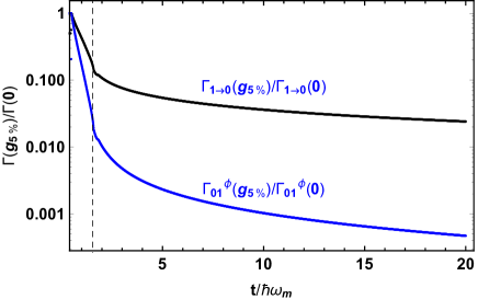
Figure 9: Ratio of the decay rate $\Gamma_{1\rightarrow 0}^{\rm qb}(g_{5\%})/\Gamma_{1\rightarrow 0}^{\rm qb}(g=0)$ and pure decoherence rate $\Gamma_{10}^{\rm qb,\phi}(g_{5\%})/\Gamma_{10}^{\rm qb,\phi}(g=0)$ as a function of $t/\hbar\omega_{\rm m}$. We assume $R^{D}=R^{\phi}=1$ and we neglect oscillator damping ($\gamma=0$). The vertical dashed line indicates the beginning of the region where the qubit becomes dominated by the two charge states, i.e. where $t<1.54\hbar\omega_{\rm m}$ (cf. also inset of Fig. 4).

VI A two-qubit gate

We have shown that a carbon-nanotube oscillator can be used as a qubit and how manipulation and read out can be performed. To use these devices to manipulate quantum information, an entangling two-qubit gate is required. In this section we discuss a possible implementation of the CNOT gate, known to be a universal gate. We follow the idea presented in Ref. [49] that exploits the coupling of two superconducting qubits to the same microwave cavity and that has been successfully implemented as reported in Ref. [50].

We consider the effective coupling generated by a microwave cavity between two nano-mechanical qubits. In the case of qubits that can be well approximated as two-level systems, the coupling to the cavity is of the form of Eq. (20): $\hbar g_{v}^{(a)}\tau_{x}^{(a)}(b+b^{\dagger})$, where the index $a$ takes the value 1 or 2 to indicate the two qubits. One can show that this induces a coupling term in the Hamiltonian $J\tau_{x}^{(1)}\tau_{x}^{(2)}$. The driving of the first qubit at the resonant frequency of the second qubit can be described by a Hamiltonian term $\hbar A\cos(\omega_{D}t)\tau_{x}^{(1)}$, where $A$ is the intensity, and $\omega_{D}=\omega_{10}^{(2)}$ the driving frequency. Taking into account the effective coupling induced between the two qubits, this translates into the term $\hbar J_{zx}\tau_{z}^{(1)}\tau_{x}^{(2)}$ in the rotating frame Hamiltonian with

$$J_{zx}={4g_{v}^{(1)}g_{v}^{(2)}A\omega_{c}\omega_{10}^{(1)}\over({\omega_{10}^{(1)}}^{2}-{\omega_{10}^{(2)}}^{2})(\omega_{c}^{2}-{\omega_{10}^{(2)}}^{2})}.$$ (42)

This is the required gate generating function, $e^{-it_{J}J_{zx}\tau_{z}^{(1)}\tau_{x}^{(2)}}=\cos(J_{zx}t_{J})-i\sin(J_{zx}t_{J})\tau_{z}^{(1)}\tau_{x}^{(2)}$, that allows the CNOT gate to be performed, modulo single-qubit rotations, in a time $t_{J}=\pi/2J_{zx}$.

One expects thus that this operation can be applied to the mechanical qubits, but since the anharmonicity is not very large, we need to investigate the contributions of the higher lying states. We proceed similarly to what we did for the dispersive coupling in section IV.6. A perturbative calculation is described in Appendix C. It gives

$$J_{zx}={Ag_{\rm ec}^{(1)}g_{\rm ec}^{(2)}\beta_{1,4}^{(2)}\over{g_{\rm ec}^{(1)}}^{2}(\omega_{c}-\omega_{10}^{(2)})}\left[\chi_{\rm m}^{(1)}(\omega_{10}^{(2)})+\chi_{\rm e}^{(1)}(\omega_{10}^{(2)})\right].$$ (43)

The expression holds for small $g/t$. We note that the coefficient diverges for $\omega_{c}=\omega_{10}^{(2)}$, while in contrast to what is found for the dispersive coupling, no divergence is present for $\omega_{c}$ close to $\delta_{00}$. We already discussed the functions $\chi_{\rm m}$ and $\chi_{\rm e}$ in IV.6, we note here that $\chi_{\rm e}^{(1)}$ diverges when its argument equals $\delta_{00}^{(1)}$ or $\delta_{11}^{(1)}$. Since in general $\omega_{10}^{(2)}\ll\delta_{00}^{(1)}\approx\delta_{11}^{(1)}$, the contribution of $\chi_{\rm e}^{(1)}$ is much smaller than that of $\chi_{\rm m}^{(1)}$, which diverges when its argument equals $\omega_{10}^{(1)}$ and $\omega_{12}^{(1)}$. Fig. 10 shows the dependence of the factor $K=J_{zx}\omega_{\rm m}^{(1)}(\omega_{c}-\omega_{10}^{(2)})/g_{\rm ec}^{(1)}g_{\rm ec}^{(2)}A$ as a function of the ratio $\omega_{\rm m}^{(2)}/\omega_{\rm m}^{(1)}$. Both the exact numerical (full line) and analytical expression Eq. (43) (dashed line) are shown. The double peak corresponds to the values for which $\omega_{10}^{(2)}$ equals either $\omega_{10}^{(1)}$ or $\omega_{21}^{(1)}$ [cf. Eq. (22)].

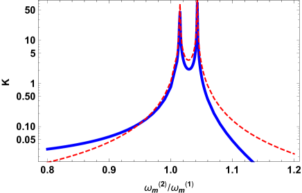
Figure 10: Coefficient $K$ of the contributions to $J_{zx}$ that diverge like $\omega_{m}^{(1)}/(\omega_{c}-\omega_{10})^{(2)})$ [divided by the two coupling constants and the driving intensity $g_{\rm ec}^{(1)}g_{\rm ec}^{(2)}A$] as a function of $\omega_{m}^{(2)}$. The full line is the numerical result and the dashed line the analytical Eq. (43). The other parameters are $g^{(1)}=g^{(2)}=1.264\hbar\omega_{m}^{(1)}$, $t^{(1)}=10\hbar\omega_{m}^{(1)}$, and $t^{(2)}=10.5\hbar\omega_{m}^{(1)}$.

This result shows that by driving the qubit 1 it is possible to induce a time dependent evolution that generates the CNOT gate.

VII Prospect for experimental implementation

The results found in the two previous sections are very promising for the experimental realization of a nanomechanical qubit. In this section we discuss possible experimental implementations using currently available technology. As discussed in the introduction, the double quantum dot can be realized in a suspendend carbon nanotube and coupled to the second mechanical flexural mode of the nanotube. Such a device has been recently measured at 2 K [29], reporting values $t/2\pi\hbar=49-96$ GHz with a tunable value of $\epsilon$, a second mechanical mode of frequency $\omega_{\rm m}/2\pi=327$ MHz with a mechanical quality factor $Q=4\cdot 10^{3}$ and a coupling constant $g/2\pi=320$ MHz. Taking these parameters, we have $t/\hbar\omega_{\rm m}$ up to 150-300, and $g/\omega_{\rm m}\approx 1$, noting that of course $t$ can be tuned to lower values. Choosing $t=7\hbar\omega_{\rm m}$, we can operate on the $g_{5\%}$ line (cf. Fig. 4) without changing other parameters. At this value of $g$, we already have a sizable reduction of both the decoherence and decay rates of the mechanical qubit $\Gamma_{1\rightarrow 0}$ and $\Gamma^{\phi}_{10}$ [cf. Fig. 9] compared to that of the charge double quantum dot. The experiment at 2 K realized with a device fabricated on a Si substrate reports an incoherent tunnelling rate $\Gamma_{1\rightarrow 0}$ estimated to $2\pi\cdot 510$ MHz, which is clearly too large to use for qubit operations, but improvements should be possible, by operating the device at 10 mK to suppress the decoherence induced by low-frequency vibrations (phonon) modes, by producing devices on sapphire substrates that host a minimal number of charge fluctuators, and by current-annealing the nanotube in-situ in the dilution fridge to remove all the contamination adsorbed on the surface of the nanotube [51]. Double-dot structures have been created in non-suspended carbon nanotubes, and have been coupled to superconducting cavities [52].

One can thus target a mechanical resonator cooled at 10 mK with $\omega_{\rm m}/2\pi$ in the range of 0.6-1 GHz using a nanotube that is shorter and/or is under mechanical tension. A value of $t/\hbar\omega_{\rm m}=10$ will then require a coupling constant of the order of $1.1\hbar\omega_{\rm m}$, which can be obtained by reducing the nanotube-gate separation and/or increasing the voltage applied on the gate electrode. With these values the reduction of the pure-dephasing decoherence rate of the mechanical qubit with respect to that of the double quantum dot will be about $10^{3}$. Assuming that the decoherence rate of the order of 3 MHz can be obtained, as was achieved in GaAs coupled double quantum dots [46] and that it is mainly limited by pure dephasing, it should be possible to implement most of the standard protocols for quantum computation using a mechanical qubit with a 3 kHz decoherence rate. Note that we did not consider the decoherence induced by the mechanical damping. Assuming a $Q$ of $10^{6}$, that has been experimentally observed in suspended carbon nanotubes [14], this would give a decoherence rate of only 500 Hz. Another possible implementation consists in using a nonsuspended GaAs double quantum dot with 3 MHz charge decoherence rate coupled to a suspended metal beam, such as a carbon nanotube.

With these parameters, one could implement a CNOT gate by choosing $\omega_{10}^{(1)}/2\pi=500$ MHz, $\omega_{10}^{(2)}/2\pi=550$ MHz (these values are reduced with respect to the oscillator mechanical frequencies), and tune the cavity to $\omega_{c}/2\pi=475$ MHz. For $t^{(a)}/\hbar\omega_{m}^{(a)}\approx 10.$, one obtains $K$ of the order of 1. We assume a coupling constant $g_{\rm ec}/2\pi=50$ MHz of the order of what reported in Ref. [53] for carbon nanotubes coupled to superconducting cavities. With these values and a drive $A/2\pi$ also of the order of 50 MHz, which is the detuning between the two qubits frequencies, one finds that $J_{zx}/2\pi\approx 2.5$ MHz, that is of the same order of what used in Ref. [50] to implement the CNOT gate in superconducting qubits.

With the chosen value of $\omega_{m}$ the typical range for $\omega_{01}/2\pi$ does not exceed 500 MHz. This is sufficient to perform single and two qubit operations, but error correction could be difficult since very low level of thermal occupation is required. In the long term, it seems feasible to increase the mechanical frequency to higher values, a qubit splitting of 1GHz is the target for implementing error correction.

VIII Quantum sensing of a static force with the nanomechanical qubit

As an important application, we discuss here the possibility of using the nanomechanical qubit for quantum sensing. A mechanical oscillator can couple to a variety of forces; independently of the nature of the force, the additional term in the Hamiltonian describing this coupling can be written as $H_{F}=Fx$, with $F$ the external force. In terms of the nanomechanical qubit operators this gives $H_{F}=F\gamma_{F}\tau_{x}/2$, with $\gamma_{F}=2{x_{\rm z}}\beta_{5}$ [cf. Eq. (12) and we introduced a factor of two for convenience in the notation]. One can then use the protocols for qubit preparation and read-out in order to measure $F$ with great sensitivity.

As a relevant example we consider here the Rabi measurement protocol, as described in Ref. [13] sec. IV.D. In a nutshell it consists in preparing the qubit in the ground state, and then let it evolve in the presence of the static force $F$ according to the Hamiltonian

$$H=\hbar(\omega_{10}\tau_{z}+\omega_{F}\tau_{x})/2,$$ (44)

with $\omega_{F}=F\gamma_{F}/\hbar$. This induces a Larmor-like precession with a Rabi frequency $\omega_{\rm R}=\sqrt{\omega_{10}^{2}+\omega_{F}^{2}}$ of the pseudo spin representing the qubit state in the Bloch sphere around the direction of the effective magnetic field vector $(\omega_{F},0,\omega_{10})$. The probability $P_{1}$ of measuring the qubit in the excited state oscillates as

$$P_{1}={\omega_{F}^{2}\over\omega_{\rm R}^{2}}\sin^{2}(\omega_{\rm R}t/2)\,.$$ (45)

For large $t$ the sine part of the expression is very sensitive to a small variation of $\omega_{\rm R}$ and thus of the force. For a detection time $t_{d}$ such that $\omega_{\rm R}t_{d}=\pi/2+k\pi$, with $k$ a large integer one finds

$$\delta P_{1}\approx\left(\omega_{F}\over\omega_{\rm R}\right)^{3}{\gamma_{F}t_{d}\over 2\hbar}F\,.$$ (46)

The sensitivity thus increases with the oscillation time $t_{d}$. This is mainly limited by the coherence time of the qubit. One also sees that in order to have a large signal it is better to have $\omega_{F}$ of the same order or larger than $\omega_{10}$. In our case this could be achieved using the gate voltage that generates an additional controllable static force to the oscillator. The most fundamental source of uncertainty in quantum sensing is the binomial fluctuation of the qubit readout outcome. Following Ref. [13] a rough estimate of the signal to noise that can be achieved with this method gives that the minimum detectable static force per unit bandwidth is

$$\delta F_{\rm min}\approx{\hbar\over\gamma_{F}\sqrt{T_{2}}},$$ (47)

where $T_{2}$ is the coherence time. Using typical values for carbon nanotube resonators $\omega_{\rm m}=2\pi\cdot 600$ MHz, $m=10^{-21}$ Kg, one has ${x_{\rm z}}\approx 4\cdot 10^{-12}$ m. Using $T_{2}\sim 50\mu$s from the 3 kHz decoherence rate for the nanotube mechanical qubit estimated in the last section, the static force sensitivity is $\sim 10^{-21}$ N/Hz^1/2. For comparison, the resolution in static force measurements is $10^{-17}$ N using optically levitated particles [54] and $10^{-12}$ N with atomic force cantilevers in high vacuum and at low temperatures [55], while a sensitivity of $10^{-15}$ N/Hz^1/2 can be achieved using optical tweezers in liquids [56]. One finds that when the electronic contribution to the decoherence can be neglected with respect to the mechanical part, then quantum sensing can reach sensitivities of the order of the standard quantum limit [57].

IX Conclusions

In conclusion we have shown that coupling a double quantum dot capacitively to the second flexural mode of a suspended carbon nanotube, and appropriately tuning the hopping amplitude between the two charge states of the quantum dot, one can introduce a strong anharmonicity in the spectrum of the mechanical mode. This enables one to address directly the first two energy quasi-mechanical eigenstates without populating the third state (cf. Fig. 4). These two states form a qubit with mainly a mechanical character. Manipulation and read-out is then possible with standard techniques, but at the same time, we found that the coupling to the environment is strongly reduced. The main benefit is the reduction by up to 3-4 orders of magnitude of the pure-dephasing rate, with respect to the double quantum dot. Combined with the expectation of improved dephasing times, this suggests the potential for nanomechanical qubits with very long coherence times. Furthermore, the production of mechanical devices using conventional microfabrication techniques is promising for scalability.

The mechanical qubit can be used to couple to a wide number of modalities for external fields, including acceleration, magnetic forces or other forces. We have shown that any fields that induce forces on the mechanical oscillator can be detected with unprecedented sensitivity, using quantum preparation and detection protocols.

We have shown that the nanomechanical qubits can be coupled to each other by microwave cavities, allowing the implementation of a CNOT gate with purely microwave control. In principle all other operations involving multiple qubits can be obtained by applying the CNOT gate and single qubit operations.

On the more technical side, we also found a unitary transformation, valid in the dispersive limit of $g/|t/\hbar-\omega_{\rm m}|\ll 1$, that maps the problem to the anharmonic oscillator, giving the explicit expressions of the main physical operators in the qubit subspace.

Appendix A Electrostatics and derivation of the coupling constants

We give here a derivation of the Hamiltonian. For this we need to calculate the electrostatic energy of the system. The only subtle point is the contribution of the voltage sources, as it is well known for the Coulomb blockade problem [58]. One needs the electrostatic energy as a function of the charges in the system, and not of the voltages; this is particularly important for the expression of the mechanical force. Following Ref. 34 (appendix A) the electrostatic problem of $N$ conductors plus a ground conductor can be treated by introducing a capacitance matrix $C^{(0)}_{ij}$ for which the charges on the conductor $i$ can be related to the potentials of the other conductors:

$$Q_{i}=\sum_{j=0}^{N}C^{(0)}_{ij}V_{j}\,.$$ (48)

Here $C^{(0)}_{ii}=\sum_{i\neq j}c_{ij}$ and $C^{(0)}_{ij}=-c_{ij}$, where $c_{ij}$ is the capacitance between conductor $i$ and $j$ and clearly ${}^{t}C=C$. We include in the list of conductors the ground with the index 0. The relation given by Eq. (48) cannot be inverted, since the capacitance matrix has vanishing determinant. This just indicates that one can shift all the potential by a constant. One can then set one of the potential to 0, say the ground, and eliminate one line of the matrix, which we choose to be that related to the charge on the ground. The $N\times N$ capacitance matrix obtained in this way, $C_{ij}$, is then invertible and one can write

$$V_{i}=\sum_{j=1}^{N}\left(C^{-1}\right)_{ij}Q_{j}\,.$$ (49)

The total energy of the system is $U=\sum_{i=0}^{N}V_{i}Q_{i}/2$. With our choice of $V_{0}=0$, it reduces to $U=\sum_{i=1}^{N}V_{i}Q_{i}/2={{}^{t}{V}}{Q}/2$, where we introduced the vector notation for the charge and the potentials. Using the capacitance matrix we have

$$U={1\over 2}{{}^{t}{V}}C{V}={1\over 2}{{}^{t}{Q}}C^{-1}{Q}.$$ (50)

In typical problems one needs to include potential sources. These can be modeled with metallic leads with a macroscopic capacitance to the ground $C_{B}\rightarrow\infty$, and the charge on this island $Q_{B}\rightarrow\infty$ with $Q_{B}/C_{B}=V_{B}$ constant. In the following, without loss of generality, we will assume that the capacitances of all sources have the same value $C_{B}$.

The relevant energy for the problem at hand is the energy expressed as a function of the charges in the metallic islands and leads. The mechanical displacement $x$ of any mechanical element of the circuit induces a change in the capacitance matrix, which acquires a dependence on the displacement $C(x)$. (For simplicity we consider a single mechanical mode whose displacement is parametrized by the variable $x$; generalization to several modes is straightforward.)

The expression for the potential energy is thus

$$U(Q,x)={1\over 2}{{}^{t}{Q}}{C(x)}^{-1}{Q}\,.$$ (51)

From this expression we can find the expression of the potential energy as a function of the charges in the dots and $x$. We can then eliminate the charges in the leads by using their potentials. For this we need to invert the matrix $C$ exploiting the large $C_{B}$ limit. Following Ref. 34 we first divide the indices in $c$ and $v$, for charge nodes and voltage sources, respectively. We can write

$$C=\left(\begin{array}[]{cc}C_{cc}&C_{cv}\\ C_{vc}&C_{vv}\end{array}\right)\,.$$ (52)

The inverse of this matrix can be written as follows

$$\left(C^{-1}\right)_{cc} = C_{cc}^{-1}+C_{cc}^{-1}C_{cv}DC_{vc}C_{cc}^{-1}$$ (53)

$$\left(C^{-1}\right)_{vc} = -DC_{vc}C^{-1}_{cc}$$ (54)

$$\left(C^{-1}\right)_{vv} = C_{vv}^{-1}(1-C_{vc}C_{cc}^{-1}C_{cv}D)$$ (55)

where $D=(C_{vv}-C_{vc}C_{cc}^{-1}C_{cv})^{-1}$. Since we eliminated the ground metal island, the only macroscopic matrix elements left are in the diagonal part of $C_{vv}\sim C_{B}$ (cf. Eq. (64) in the following). We can then simplify greatly the inverse since to leading order in $C_{B}$ one has $D=1/C_{B}$,

$$\left(C^{-1}\right)_{cc} = C_{cc}^{-1},$$ (56)

$$\left(C^{-1}\right)_{vc} = -C_{vc}C^{-1}_{cc}/C_{B},$$ (57)

$$\left(C^{-1}\right)_{vv} = 1/C_{B}.$$ (58)

This allows to express the energy as follows:

$$U={1\over 2}{{}^{t}Q_{c}}C_{cc}^{-1}Q_{c}-{{}^{t}Q_{c}}C_{cc}^{-1}C_{cv}Q_{v}/C_{B}+{1\over 2}{{}^{t}Q_{v}}Q_{v}/C_{B},$$ (59)

but $Q_{v}/C_{B}=V_{v}$ are the sources voltages and the last term is independent of $Q_{c}$. We thus have

$$U={1\over 2}{{}^{t}Q_{c}}C_{cc}^{-1}Q_{c}-{{}^{t}Q_{c}}C_{cc}^{-1}C_{cv}V_{v}\,.$$ (60)

A.1 Couplings

From this expression we can derive the coupling to the mechanical displacement and to the voltage applied to a nearby gate electrode. For this, we include the $x$ dependence of the capacitances and the substitution $V_{v}=V_{v}^{\rm DC}+V_{v}^{\rm AC}$, where $V_{v}^{\rm DC}$ is the static part and $V_{v}^{\rm AC}$ the oscillating part of the voltage. If a gate electrode is part of an electromagnetic cavity, one can obtain the coupling to the photon creation and destruction operators via the substitution $V_{v}^{\rm AC}=V_{v}^{\rm z}(b_{v}+b_{v}^{\dagger})$, where $V_{v}^{\rm z}$ is the zero-point voltage of the cavity and $b_{v}$ the destruction operator for the photons.

We now need a description in terms of the charge fields. Let us associate to each charge variation $\delta q^{i}_{c}$ the occupation operator $n_{i}$ with eigenvalues 0 or 1 so that the operator for the total number of charges can be written as $Q_{c}=Q_{c}^{0}+\sum_{i}n_{i}\delta q^{i}_{c}$. The index $i$ can take into account spin or other degrees of freedom and we included a back-ground frozen charge $Q_{c}^{0}$. By including this expression into (60), at lowest order in $x$ we obtain

$$U = U_{C}+x\sum_{i}n_{i}\left(\lambda^{\rm em}_{i}+\sum_{j\neq i}n_{j}\lambda^{\rm em}_{ij}\right)$$ (61)

$$+\sum_{i}n_{i}\lambda^{\rm ev}_{iv}V^{AC}_{v}+x\lambda^{\rm mv}_{v}V^{AC}_{v}$$

where

$$U_{C}=\sum_{i}n_{i}{{}^{t}\delta q^{i}_{c}}C_{cc}^{-1}\left(Q_{c}^{0}-C_{cv}V_{v}^{DC}+\sum_{j}{1\over 2}\delta q_{c}^{j}n_{j}\right)$$ (62)

is the pure Coulomb part and the other three terms describe the interaction between the three degrees of freedom $x$, $V^{\rm AC}$, and $n_{i}$, which are associated with the indices m, v, and e, respectively. (We discarded the constant $U_{0}={{}^{t}Q^{0}_{c}}C_{cc}^{-1}Q^{0}_{c}/2-{{}^{t}Q^{0}_{c}}C_{cc}^{-1}C_{cv}V_{v}^{DC}$.) Here

$$\lambda^{\rm em}_{i}=\partial_{x}\left[\left({{}^{t}Q^{0}_{c}}+{{}^{t}\delta q_{c}^{i}\over 2}\right)C_{cc}^{-1}-V^{DC}_{v}C_{vc}C_{cc}^{-1}\right]{\delta q_{c}^{i}}$$ (63)

and $\lambda^{\rm em}_{ij}={{}^{t}\delta q_{c}^{i}}\partial_{x}C_{cc}^{-1}{\delta q_{c}^{j}}/2$ are the electromechanical couplings, $\lambda^{\rm ev}_{iv}=-{{}^{t}\delta q_{c}^{i}}C_{cc}^{-1}C_{cv}$ the voltage-electron coupling, and $\lambda^{\rm mv}_{v}=-{{}^{t}Q^{0}_{c}}\partial_{x}(C_{cc}^{-1}C_{cv})$ the mechanical oscillator-voltage coupling.

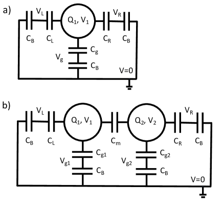
Figure 11: Network of capacitances representing the (a) single- and (b) double-dot circuit. The capacitances $C_{B}$ are used to model the voltage sources.

A.2 Single- and double-dot cases

We now consider two examples.

(i) The single dot. In this case we have 4 metallic entities, one for the dot, 3 for the left, right and gate leads [cf. Fig. 11 (a)]. The matrix $C$ reads:

$$C=\left(\begin{array}[]{cccc}C_{1}&-C_{R}&-C_{L}&-C_{g}\\ -C_{R}&C_{B}+C_{R}&0&0\\ -C_{L}&0&C_{B}+C_{L}&0\\ -C_{g}&0&0&C_{B}+C_{g}\end{array}\right)$$ (64)

with obvious notation for the capacitances and with $C_{1}=C_{L}+C_{R}+C_{g}$. This gives $C_{cc}=C_{1}$, $C_{cv}=-(C_{R},C_{L},C_{g})$, and $C_{vv}=C_{B}+{\rm diag}(C_{R},C_{L},C_{g})$. We assume that only $C_{g}$ depends on $x$, this gives $\partial_{x}C_{cc}=\partial_{x}C_{g}=C_{g}^{\prime}$ and $\partial_{x}C_{cv}=-C_{g}^{\prime}(0,0,1)$. We also have $\delta q_{c}^{i}=-e$ (with $e$ the electron charge) and for simplicity we report the expressions for $V_{L}=V_{R}=0$. We then have for the couplings

$$\lambda^{\rm em}_{i}=eC_{g}^{\prime}[Q_{0}-(C_{1}-C_{g})V_{g}-e/2]/C_{1}^{2},$$ (65)

$\lambda^{\rm em}_{ij}=-e^{2}C_{g}^{\prime}/(2C_{1}^{2})$, $\lambda^{\rm mv}_{v}=-C_{g}^{\prime}Q_{0}(C_{R},C_{L},C_{g}-C_{1})/C_{1}^{2}$. The last coupling constant is related to $\lambda^{\rm em}$. Using the value of $Q_{0}$ that minimizes the electrostatic energy: $Q_{0}=-C_{g}V_{g}$ and assuming $|Q_{0}|\gg e$ one obtains for the single-dot coupling constant $\lambda^{\rm em}_{i}=-eC_{g}^{\prime}V_{g}/C_{1}$. Note also that in this limit $\lambda^{\rm em}_{ij}/\lambda^{\rm em}_{i}=e/2C_{1}V_{g}\ll 1$.

(ii) Double dot. Let us consider a double dot, with each dot coupled to a gate voltage [cf. Fig. 11 (b)]. The capacitance matrix is:

$$C_{cc} = \left(\begin{array}[]{cc}C_{1}&-C_{m}\\ -C_{m}&C_{2}\end{array}\right)\,,$$ (68)

$$C_{cv} = -\left(\begin{array}[]{cccc}C_{L}&C_{g1}&0&0\\ 0&0&C_{g2}&C_{R}\end{array}\right)\,,$$ (71)

and $C_{vv}=C_{B}+{\rm diag}(C_{L},C_{g1},C_{g2},C_{R})$. Here $C_{1}=C_{L}+C_{m}+C_{g1}$ and $C_{2}=C_{R}+C_{m}+C_{g2}$ We can distinguish two types of $n$ operators, one for the dot 1 ($n_{1}$) and the other for the dot 2 ($n_{2}$). We have $\delta q_{c}^{1}=(-e,0)$ and $\delta q_{c}^{2}=(0,-e)$. For simplicity in the following we assume a symmetric situation $C_{L}=C_{R}=C$, $V_{L}=V_{R}=0$, $C_{1}=C_{2}=C_{S}$ $Q_{c}^{0}=(Q_{0},Q_{0})$, and $V_{v}=(0,V_{g1},V_{g2},0)$. For our specific problem, for which the interesting mechanical mode is the second one, we assume that $C_{g1}(x)=C_{g2}(-x)$ by symmetry, so that $C_{g1}^{\prime}=-C_{g2}^{\prime}$. With this hypothesis we find for the coupling constants:

$$\lambda^{\rm em}_{1}+\lambda^{\rm em}_{2} = -{eC_{g}^{\prime}(C+2C_{m})(V_{g1}-V_{g2})\over C_{S}^{2}-C_{m}^{2}}$$

$$\lambda^{\rm em}_{1}-\lambda^{\rm em}_{2} = {eC_{g}^{\prime}[2Q_{0}-e-C(V_{g1}+V_{g2})]\over C_{S}^{2}-C_{m}^{2}}$$

$$\lambda^{\rm ev}_{1v} = -e{(CC_{S},C_{g}C_{S},C_{g}C_{m},CC_{m})\over C_{S}^{2}-C_{m}^{2}}$$

$$\lambda^{\rm ev}_{2v} = -e{(CC_{m},C_{g}C_{m},C_{g}C_{S},CC_{S})\over C_{S}^{2}-C_{m}^{2}}$$

$$\lambda^{\rm mv}_{v} = Q_{0}C_{g}^{\prime}{(-C,2C_{m}+C,-2C_{m}-C,C)\over C_{S}^{2}-C_{m}^{2}}$$

and $\lambda^{\rm em}_{12}=0$. For $V_{g1}=V_{g2}=V_{g}$ $\lambda^{\rm em}_{1}=-\lambda^{\rm em}_{2}=\lambda^{\rm em}$ leading to the Hamiltonian term that we used in the main text: $\lambda^{\rm em}x(n_{1}-n_{2})$. When we reduce the Hilbert space to the two charge states $(1,0)$ and $(0,1)$, this Hamiltonian term can be written as $\lambda^{\rm em}x\sigma_{z}\equiv-\hbar g(x/{x_{\rm z}})\sigma_{z}$. In this basis $n_{1}=(\sigma_{z}+\mathds{1})/2$ and $n_{2}=(\mathds{1}-\sigma_{z})/2$. This gives

$$g={eC^{\prime}_{g}[2CV_{g}+e-2Q_{0}]x_{z}\over 2\hbar(C_{S}^{2}-C_{m}^{2})}\,.$$ (72)

For the case $Q_{0}=-C_{g}V_{g}$, $|Q_{0}|\gg e$, and $C_{m}\ll C_{S}$, we obtain $g=eC_{g}^{\prime}V_{g}x_{z}/\hbar C_{S}$, that coincides with the single dot coupling constant. We also have the coupling of the charge of the dots to the voltages of the gate electrodes:

$$H^{\rm ev}={eC_{g}\over 2}\left[\mathds{1}{V_{g1}^{\rm AC}+V_{g2}^{\rm AC}\over C_{S}-C_{m}}+\sigma_{z}{V_{g1}^{\rm AC}-V_{g2}^{\rm AC}\over C_{S}+C_{m}}\right]\,.$$ (73)

Finally the direct coupling between the mechanical oscillator and the voltages of the gate electrodes is:

$$H^{\rm mv}=Q_{0}C_{g}^{\prime}{C+2C_{m}\over C_{S}^{2}-C_{m}^{2}}x(V_{g1}^{\rm AC}-V_{g2}^{\rm AC})\,.$$ (74)

In order to compare the last two coupling constants we can write this part of the Hamiltonian as follows

$$H=\left[\lambda^{\rm ev}\sigma_{z}+\lambda^{\rm mv}{x_{\rm z}}(a+a^{\dagger})\right]V_{g12}^{AC}$$ (75)

with $\lambda^{\rm ev}=eC_{g}/[2(C_{S}+C_{m})]$, $\lambda^{\rm mv}=Q_{0}C_{g}^{\prime}(C+2C_{m})/(C_{S}^{2}-C_{m}^{2})$, $V_{g12}^{AC}=V_{g1}^{\rm AC}-V_{g2}^{\rm AC}$, and we used $x={x_{\rm z}}(a+a^{\dagger})$. The ratio of the two coupling constant is then of the order of

$${\lambda^{\rm mv}{x_{\rm z}}\over\lambda^{\rm ev}}={Q_{0}\over e}{C_{g}^{\prime}\over 2C_{g}}{x_{\rm z}}{C+2C_{m}\over C_{S}-C_{m}}\,.$$ (76)

In general this ratio is small $\sim(Q_{0}/e)({x_{\rm z}}/L)$ where $L=C_{g}/C_{g}^{\prime}$ is typically of the order of the distance of the nanotube from the gate. Thus the oscillating voltage field couples mainly to the charge degree of freedom.

Appendix B Mapping of the Hamiltonian on the anharmonic oscillator in the dispersive regime

In this Appendix we show that the Hamiltonian for the system we are considering given by Eq. (1) can be mapped in the dispersive regime on the Hamiltonian of an anharmonic oscillator. We begin by considering $H$ for $\epsilon=0$. It reduces to $H=t\sigma_{x}/2+\hbar\omega_{\rm m}a^{\dagger}a-\hbar g(a+a^{\dagger})\sigma_{z}$. Performing a rotation of $\pi/2$ around the $y$-axis in the charge space with the operator $U_{r}=e^{-i\pi\sigma_{y}/4}=(1-i\sigma_{y})/\sqrt{2}$, one has that $U^{\dagger}_{r}\sigma_{x}U_{r}=\sigma_{z}$ and $U^{\dagger}_{r}\sigma_{z}U_{r}=-\sigma_{x}$, with $\sigma_{y}$ left unchanged. The Hamiltonian is then in the standard form for the Rabi model:

$$H_{1}=U_{r}^{\dagger}HU_{r}={t\over 2}\sigma_{z}+\hbar\omega_{\rm m}a^{\dagger}a+\hbar g(a+a^{\dagger})\sigma_{x}.$$ (77)

This model has a long history describing the coupling of electromagnetic radiation to a two-level system, but only very recently it has been diagonalized analytically [59]. In practice it is difficult to make use of this solution, but for the case considered in the present paper, an approximate solution, which holds in the so called dispersive limit of $|t-\hbar\omega_{\rm m}|\ll g$, could be sufficient to obtain an accurate description of the system. As described in Ref. 60, it exists a unitary transformation $D_{1}$ such that

$$H_{2}=D_{1}^{\dagger}H_{1}D_{1}=t{\sigma_{z}\over 2}+{\hbar\omega_{\rm m}\over 4}({\hat{p}}^{2}+{\hat{x}}^{2})+\sigma_{z}{\hat{x}}^{2}{t\hbar g^{2}\over\Delta^{2}}+\dots$$ (78)

where we recall $\Delta^{2}=t^{2}-(\hbar\omega_{\rm m})^{2}$, ${\hat{x}}=a^{\dagger}+a$, and ${\hat{p}}=i(a^{\dagger}-a)$, with $[{\hat{x}},{\hat{p}}]=2i$. The Hamiltonian is quadratic in ${\hat{x}}$ and ${\hat{p}}$ and commutes with $\sigma_{z}$. It can thus be diagonalized

$$H_{2}=t\sigma_{z}/2+\sum_{\sigma=\pm}[\hbar\omega_{\sigma}\pi_{\sigma}(1/2+a_{\sigma}^{\dagger}a_{\sigma})],$$ (79)

where

$${\hat{x}}=\sum_{\sigma}\xi_{\sigma}(a_{\sigma}^{\dagger}+a_{\sigma})\pi_{\sigma},\quad{\hat{p}}=\sum_{\sigma}\xi_{\sigma}^{-1}i(a_{\sigma}^{\dagger}-a_{\sigma})\pi_{\sigma},$$ (80)

with

$$\omega_{\sigma}=\omega_{\rm m}[1+4\sigma t\hbar g^{2}/\omega_{\rm m}\Delta^{2}]^{1/2}$$ (81)

the mechanical frequency of each branch, $\pi_{\sigma}=(1+\sigma\sigma_{z})/2$ the projector on the $\sigma$ branch, $\xi_{\sigma}=(\omega_{\rm m}/\omega_{\sigma})^{1/2}$, and $[a_{\sigma},a^{\dagger}_{\sigma^{\prime}}]=\delta_{\sigma,\sigma^{\prime}}$. Note that this result reduces to the Born-Oppenheimer picture for $\hbar\omega_{\rm m}/t\rightarrow 0$. It describes two harmonic oscillators, with different resonating frequencies, the lower branch being softened and the upper being hardened by the interaction.

The transformation found in Ref. [60] allows to simplify the Hamiltonian only at order 2 in $\hbar g/|t-\hbar\omega_{\rm m}|$. For our purposes we need a transformation allowing to obtain the form of the Hamiltonian up to the quartic terms in ${\hat{x}}$. For this reason we look for an higher-order unitary transformation $D$ that allows to map $H_{1}$ to $H_{T}=D^{\dagger}H_{1}D$ (the full unitary transformation acting on $H$ includes the rotation $U=U_{r}D$) with $H_{T}$ given by Eq. (5) of the main text valid at order four in $g/(t/\hbar-\omega_{\rm m})$.

In general one can express any unitary transformation as $D=e^{A}$, where $A=-A^{\dagger}$. We begin by expressing the transformation of Ref. [60] in terms of the operators ${\hat{x}}$ and ${\hat{p}}$:

$$A_{1}={i\hbar g\over\Delta^{2}}(t\sigma_{y}x+\hbar\omega_{\rm m}\sigma_{x}p)\,.$$ (82)

The transformed operators can be found using the standard relation:

$$e^{A}Oe^{-A}=\sum_{n}{1\over n!}C^{O}_{n}\,,$$ (83)

with $C^{O}_{n}=[A,C^{O}_{n-1}]$, and $C^{O}_{0}=O$. Performing the expansion at order 2 for $O=H_{1}$ and $A=A_{1}$ one obtains the expression for $H_{2}$. Performing the expansion at order 4 generates the sought terms $x^{4}$, but also other terms proportional to $x^{3}\sigma_{x}$, $xpx\sigma_{y}$ and $x^{2}p^{2}\sigma_{z}$. In order to eliminate these terms we add two terms to the $A_{1}$ operator so that $A=A_{1}+g^{3}A_{3}+g^{4}A_{4}$. By inspection of the terms generated one can realize that $A_{3}$ should involve only cubic terms in ${\hat{x}}$ and ${\hat{p}}$, while $A_{4}$ only quartic terms. These terms are multiplied by any of the three Pauli matrices and the unit matrix. This leaves 12 free parameters for $A_{3}$ and 15 free parameters for $A_{4}$. By imposing that the cubic and quartic terms (apart from $x^{4}$) vanish, we find an explicit expression for $A_{3}$ and $A_{4}$

$$A_{3} = {4it\hbar^{3}\over 3\Delta_{3}^{2}\Delta^{6}}\left[4\sigma_{x}t\hbar\omega_{\rm m}[{\hat{x}}{\hat{p}}{\hat{x}}(3\hbar^{2}\omega_{\rm m}^{2}-t^{2})+2\hbar^{2}\omega_{\rm m}^{2}{\hat{p}}^{3}]\right.$$

$$\left.+\sigma_{y}[8t^{2}\hbar^{2}\omega_{\rm m}^{2}{\hat{p}}{\hat{x}}{\hat{p}}+{\hat{x}}^{3}(-t^{4}+6t^{2}\hbar^{2}\omega_{\rm m}^{2}+3\hbar^{4}\omega_{\rm m}^{4})]\right]$$

$$A_{4} = {i\sigma_{z}({\hat{x}}^{3}{\hat{p}}+{\hat{p}}{\hat{x}}^{3})t\hbar^{5}\omega_{\rm m}(11t^{2}-3\hbar^{2}\omega_{\rm m}^{2})\over 6\Delta_{3}^{2}\Delta^{6}}\,.$$ (85)

This leads to the Hamiltonian (5) with the coefficients given by Eqs. (6)-(7). Note that the coefficients $\alpha_{1}$ and $\alpha_{2}$ are very close to one in the limit $\hbar\omega_{\rm m}/t\ll 1$ since the correction scale like $(\hbar g/t)^{4}$ and $\hbar^{4}g^{4}\omega_{\rm m}^{2}/t^{6}$.

We thus have shown that the Born-Oppenheimer picture gives a qualitatively correct description of the problem, even deep in the quantum regime when $\hbar\omega_{\rm m}$ is not negligible in front of $t$. This implies a non-trivial unitary transformation that, in contrast with the Born-Oppenheimer picture, mixes the mechanical and charge degrees of freedom. The second important difference is that the coefficients for the quadratic and quartic terms differs from the ones of the semiclassical case. These are of course important if a quantitative description of the anharmonicity is needed.

B.1 Form of the operators in the qubit Hilbert space

In order to study the decoherence and the way in which the mechanical qubit can be manipulated it is important to obtain the projection of the main operators on the Hilbert subspace formed by the lowest two Hamiltonian eigenstates. This of course can be done numerically in a straightforward way, but it is also useful to have simple, though approximate, expressions for the form of the operators. For this purpose one can apply the unitary transformations $U=U_{r}D$, introduced above, to find the expression of the relevant operators in the base for which the Hamiltonian reduces to the form (5) at order $g^{4}$. We are interested by the Pauli matrices for the charge sector and the ${\hat{x}}$ and ${\hat{p}}$ operators, for the oscillator sector. Let’s define $O^{T}=U^{\dagger}OU$. We obtain:

$$\sigma_{x}^{T} = \sigma_{z}+2\hbar g{{\hat{p}}\sigma_{y}\hbar\omega_{\rm m}-\sigma_{x}{\hat{x}}t\over\Delta^{2}}-2\hbar^{2}g^{2}{\sigma_{z}{\hat{x}}^{2}t^{2}+2t\hbar\omega_{\rm m}+{\hat{p}}^{2}\sigma_{z}(\hbar\omega_{\rm m})^{2}\over\Delta^{4}}+o(g^{3}),$$ (86)

$$\sigma_{y}^{T} = \sigma_{y}-2\hbar^{2}g\omega_{\rm m}{{\hat{p}}\sigma_{x}\over\Delta^{2}}+\hbar^{3}g^{2}\omega_{\rm m}{\sigma_{x}t({\hat{x}}{\hat{p}}+{\hat{p}}{\hat{x}})-2{\hat{p}}^{2}\sigma_{y}\hbar\omega_{\rm m}\over\Delta^{4}}+o(g^{3}),$$ (87)

$$\sigma_{z}^{T} = -\sigma_{x}-2\hbar gt{{\hat{x}}\sigma_{z}\over\Delta^{2}}+\hbar^{2}g^{2}t{2\sigma_{z}{\hat{x}}^{2}t-\sigma_{y}\hbar\omega_{\rm m}({\hat{x}}{\hat{p}}+{\hat{p}}{\hat{x}})\over\Delta^{4}}+o(g^{3}),$$ (88)

$${\hat{x}}^{T} = {\hat{x}}+2\hbar^{2}g\omega_{\rm m}{\sigma_{x}\over\Delta^{2}}+2\hbar^{3}g^{2}{\sigma_{z}{\hat{x}}t\omega_{\rm m}\over\Delta^{4}}+o(g^{3})\,,$$ (89)

$${\hat{p}}^{T} = {\hat{p}}-2\hbar gt{\sigma_{y}\over\Delta^{2}}+2\hbar^{3}g^{2}{\sigma_{z}{\hat{p}}t\omega_{\rm m}\over\Delta^{4}}+o(g^{3})\,.$$ (90)

The projection in the subspace of the first two-excited states can be readily calculated by neglecting the quartic term of the Hamiltonian given by Eq. (5). This implies a scaling of the ${\hat{x}}$ and ${\hat{p}}$ operators by the factor $\xi=\xi_{-}$ defined by Eq. (9): ${\hat{x}}\rightarrow\xi{\hat{x}}$ and ${\hat{p}}\rightarrow{\hat{p}}/\xi$. The result at order 4 in $g$ gives that only 6 components are non-vanishing, out of the possible 16. These are given by Eq. (11) and Eq. (12) in the main text. The expression for the $\beta$ coefficients is given in the main text (LABEL:beta1)-(18) to order $g^{2}$. From these expression one can see how the different degrees of freedom are mixed by the interaction. For instance, the displacement acquires a $\sigma_{x}$ component, which in this basis is the charge operator. On the other side the charge operator $\sigma_{z}$ acquires a component of the displacement operator. We give here the $g^{3}$ and $g^{4}$ terms (we use $\hbar=1$ in these expressions):

$$\beta_{14} = \frac{16t\left(6\omega_{\rm m}^{2}t^{3}\left(9\xi^{4}+2\right)\xi^{4}-4\omega_{\rm m}^{3}t^{2}\left(15\xi^{4}+16\right)\xi^{2}+9\omega_{\rm m}^{4}t\left(3\xi^{8}+4\xi^{4}+8\right)-18\omega_{\rm m}^{5}\xi^{6}+14\omega_{\rm m}t^{4}\xi^{6}-9t^{5}\xi^{8}\right)}{3\Delta^{8}\Delta_{3}^{2}\xi^{4}}$$ (91)

$$\beta_{24} = \frac{16t\left(-4\omega_{\rm m}^{2}t^{3}\left(9\xi^{4}+2\right)\xi^{4}+2\omega_{\rm m}^{3}t^{2}\left(15\xi^{4}+16\right)\xi^{2}-6\omega_{\rm m}^{4}t\left(3\xi^{8}+4\xi^{4}+8\right)+9\omega_{\rm m}^{5}\xi^{6}-7\omega_{\rm m}t^{4}\xi^{6}+6t^{5}\xi^{8}\right)}{3\Delta^{8}\Delta_{3}^{2}\xi^{4}}$$ (92)

$$\beta_{33} = \frac{96\omega_{\rm m}^{3}t^{2}\left(\xi^{4}+2\right)-32\omega_{\rm m}t^{4}\xi^{4}}{3\Delta^{6}\Delta_{3}^{2}\xi^{3}}$$ (93)

$$\beta_{43} = \frac{8\left(2\omega_{\rm m}^{2}t^{3}\left(9\xi^{4}+4\right)+9\omega_{\rm m}^{4}t\xi^{4}-3t^{5}\xi^{4}\right)}{3\Delta^{6}\Delta_{3}^{2}\xi}$$ (94)

$$\beta_{54} = \frac{2\omega_{\rm m}t\left(3\xi^{4}\left(-58\omega_{\rm m}^{2}t^{2}-15\omega_{\rm m}^{4}+9t^{4}\right)-64\omega_{\rm m}^{2}t^{2}-96\omega_{\rm m}t\xi^{2}(t-\omega_{\rm m})(\omega_{\rm m}+t)\right)}{3\Delta^{8}\Delta_{3}^{2}\xi}$$ (95)

$$\beta_{64} = \frac{2\omega_{\rm m}t\left(\xi^{4}\left(-66\omega_{\rm m}^{2}t^{2}-27\omega_{\rm m}^{4}+29t^{4}\right)-192\omega_{\rm m}^{2}t^{2}+96\omega_{\rm m}t\xi^{2}(t-\omega_{\rm m})(\omega_{\rm m}+t)\right)}{3\Delta^{8}\Delta^{2}\xi^{3}}.$$ (96)

Appendix C Microwave cavity coupled to one and two qubits

Let us consider a generic system coupled linearly through the operator $S$ to a microwave cavity. The Hamiltonian can be written as:

$$H/\hbar=H_{S}/\hbar+\omega_{c}b^{\dagger}b+S(b^{\dagger}+b),$$ (97)

where $b$ are the photon destruction operators, $\omega_{c}$ the cavity resonating angular velocity, $H_{S}$ the unspecified system Hamiltonian. We assume that $S$ acts only in the system Hilbert space. Let us also define the energy eigenvalues of $H_{S}$: $\hbar\epsilon_{i}$ with eigenstates $|i\rangle$ such that $H_{S}|i\rangle=\hbar\epsilon_{i}|i\rangle$.

Assuming that $S$ is small we find the modification of the eigenvalues and eigenvectors of the full system by standard second-order perturbation theory. The unperturbed eigenvectors of the system plus cavity are $|im\rangle$ with eigenvalue $\varepsilon_{im}^{(0)}=\epsilon_{i}+m\omega_{c}$. The first order correction vanishes. The second order reads:

$$\varepsilon^{(2)}_{im}=\sum_{j}|S_{ij}|^{2}\left[{m\over\epsilon_{ij}+\omega_{c}}+{m+1\over\epsilon_{ij}-\omega_{c}}\right],$$ (98)

with $\epsilon_{ij}=\epsilon_{i}-\epsilon_{j}$. The linear part in $m$ of this expression gives the renormalization of the resonator frequency. It normally depends on the system state $i$:

$$\Delta\omega_{i}=\sum_{j}|S_{ij}|^{2}{2\epsilon_{ij}\over(\epsilon_{ij}^{2}-\omega_{c}^{2})}.$$ (99)

Thus the dispersive coupling $\chi$ [cf. Eq. (21)] defined as half the variation of the resonating frequency for a transition from the ground to the first excited state of the system is:

$$\chi=(\Delta\omega_{1}-\Delta\omega_{0})/2.$$ (100)

C.1 Dispersive coupling for a single qubit

As a simple example one can consider the case $H_{S}/\hbar=\epsilon_{10}\tau_{z}/2$ and $S=g_{\rm v}\tau_{x}$. One finds $\Delta\omega_{1}=-\Delta\omega_{0}=2g_{\rm v}^{2}\epsilon_{10}/(\epsilon_{10}^{2}-\omega_{c}^{2})$. For $\omega_{c}$ close to $\epsilon_{10}$ one then recovers the value of $\chi=g_{\rm v}^{2}/(\epsilon_{10}-\omega_{c}^{2})$ entering Eq. (21).

Using Eq. (99) we can now find the dispersive coupling for the nanomechanical qubit. We perform the unitary transformation given by $D_{1}U_{r}$ and we use for $H_{S}$ the quadratic Hamiltonian $H_{2}$ given in Eq. (78). In this case the eigenvectors are $|n\sigma\rangle$ with eigenvalues $E_{n\sigma}=\hbar n\omega_{\sigma}+t_{R}\sigma/2$ [here $t_{R}=t+\hbar(\omega_{+}-\omega_{-})$ is the hopping amplitude renormalized by the zero point energies]. The system couples to the cavity through the charge and the displacement operators, but since the latter coupling is much smaller than the former, we consider in the following only the charge operator $\sigma_{z}$. We write the coupling operator in the new basis: $S=g_{\rm ec}D_{1}^{\dagger}U_{r}^{\dagger}\sigma_{z}U_{r}D_{1}$. At lowest order it reads (cf. Eq. (88)):

$${S\over g_{\rm ec}}=\sigma_{x}+{2\hbar gt\over\Delta^{2}}\left(\begin{array}[]{cc}(a_{+}+a_{+})\xi_{+}&0\\ 0&(a_{-}+a_{-})\xi_{-}\end{array}\right)+\dots.$$ (101)

Substituting $S$ into Eq. (99) and Eq. (100) with the two lowest lying states $|0-\rangle$ and $|1-\rangle$, we find $\chi=\chi_{\rm m}+\chi_{\rm e}$ with

$$\chi_{\rm m}=2g_{\rm ec}^{2}\beta_{4,1}^{2}{(\omega_{21}-\omega_{10})(\omega_{c}^{2}+\omega_{10}\omega_{21})\over(\omega_{c}^{2}-\omega_{21}^{2})(\omega_{c}^{2}-\omega_{10}^{2})}$$ (102)

and

$$\chi_{\rm e}=g_{ec}^{2}{(\delta_{11}-\delta_{00})(\omega_{c}^{2}+\delta_{11}\delta_{00})\over(\omega_{c}^{2}-\delta_{11}^{2})(\omega_{c}^{2}-\delta_{00}^{2})},$$ (103)

where we recall that $\beta_{4,1}=2\hbar gt\xi_{-}/\Delta^{2}$ and $\delta_{nm}=(E_{n+}-E_{n-})/\hbar$. Note that the expression in Eq. (102) vanishes if the lowest order approximation for the energy eigenvalues is used. A non-linearity is needed in order to have a finite dispersive coupling. For this reason we do not specify the values of $\omega_{nm}$ and $\delta_{nm}$ for the moment. Both expressions have a divergent behaviour: $\chi_{\rm m}$ for $\omega_{c}$ close to either $\omega_{01}$ or $\omega_{21}$, $\chi_{\rm e}$ for $\omega_{c}$ close to either $\delta_{00}$ or $\delta_{11}$. This allows us to write the approximate Eqs. (22) and (23) in the main text.

C.2 Coupling two-qubits via the cavity

We apply now this approach to study two nanomechanical qubits coupled to the same microwave cavity. Our main goal is to find the expression of a system operator $F$, acting only in the system Hilbert space, on the eigenvectors basis of the coupled system of the two qubits plus the microwave cavity. We are looking at the $m$-independent part, that gives the change of the operator in the system subspace. Applying second order perturbation theory with the same notation of before we obtain

$$\left\langle i^{\prime}m|F|im\right\rangle=F_{i^{\prime}i}+\sum_{k,l\neq i^{\prime}}{S_{i^{\prime}k}S_{kl}F_{li}\over(\epsilon_{i^{\prime}k}-\omega_{c})\epsilon_{i^{\prime}l}}$$

$$+\sum_{k,l\neq i}{F_{i^{\prime}l}S_{lk}S_{ki}\over(\epsilon_{ik}-\omega_{c})\epsilon_{il}}+\sum_{kk^{\prime}}{S_{i^{\prime}k}F_{kk^{\prime}}S_{k^{\prime}i}\over(\epsilon_{i^{\prime}k}-\omega_{c})(\epsilon_{ik^{\prime}}-\omega_{c})}$$

$$-{F_{i^{\prime}i}\over 2}\left[\sum_{j\neq i}{|S_{ij}|^{2}\over(\epsilon_{ij}-\omega_{c})^{2}}+\sum_{j\neq i^{\prime}}{|S_{i^{\prime}j}|^{2}\over(\epsilon_{i^{\prime}j}-\omega_{c})^{2}}\right].$$ (104)

As a simple application we can consider a system composed of two pure two-level systems qubits: $H_{S}=\sum_{a=1,2}\hbar\epsilon_{10}^{(a)}\tau_{z}^{(a)}/2$, with $S=\sum_{a=1,2}g_{\rm v}^{(a)}\tau_{x}^{(a)}$. When a drive is applied to qubit 1 this can be modeled by a term in the Hamiltonian $\hbar A\cos(\omega_{D}t)\tau_{x}^{(1)}$. We thus look how $F=\tau_{x}$ reads in the Hamiltonian eigenvector basis. Using Eq. (104) we find that

$$F=F_{x0}\tau_{x}^{(1)}+F_{0x}\tau_{x}^{(2)}+F_{zx}\tau_{x}^{(1)}\tau_{x}^{(2)},$$ (105)

with $F_{zx}$ given by the expression (42) for $J_{zx}$ with $\omega_{10}\rightarrow\epsilon_{10}$ and $A\rightarrow 1$.

We consider now the case of a nanomechanical qubit. To evaluate Eq. (104) we use the same method applied for the single qubit. The coupling operator is now $S=\sum_{a=1,2}g_{\rm ec}^{(a)}\sigma_{z}^{(a)}$. The eigenstates of the composite system can be labeled with the four indices $\{n_{1},\sigma_{1};n_{2}\sigma_{2}\}$ with eigenvalues $E_{n_{1},\sigma_{1}}+E_{n_{2},\sigma_{2}}$. As before we assume we have the exact expressions for the eigenvalues and we use the matrix elements given by the quadratic Hamiltonian. We look for the contributions leading to the operator $\tau_{z}^{(1)}\tau_{x}^{(2)}$. We find that also in this case $F$ has the form of Eq. (105).

At lowest order in the electromechanical coupling constants these terms are generated by selecting the contribution of two $\sigma_{x}^{(1)}$ and one ${\hat{x}}^{(2)}$ operators entering the matrix elements of $F$ and $S$. They have dominant divergent terms in $1/(\omega_{c}-\omega_{10}^{(2)})$. Collecting them one obtains:

$$F_{zx}^{\rm e}={g_{\rm ec}^{(1)}g_{\rm ec}^{(2)}\beta_{4,1}^{(2)}\over\omega_{10}^{(2)}-\omega_{c}}\left[{\delta_{11}^{(1)}\over{\delta_{11}^{(1)}}^{2}-{\omega_{10}^{(2)}}^{2}}-{\delta_{00}^{(1)}\over{\delta_{11}^{(1)}}^{2}-{\omega_{10}^{(2)}}^{2}}\right]$$ (106)

that close to the resonance can be written as

$$F_{zx}^{\rm e}\approx-{g_{\rm ec}^{(1)}g_{\rm ec}^{(2)}\beta_{1,4}^{(2)}\over\omega_{10}^{(2)}-\omega_{c}}{(\delta_{11}^{(1)}-\delta_{00}^{(1)})({\delta_{00}^{(1)}}^{2}+{\omega_{10}^{(2)}}^{2})\over({\delta_{00}^{(1)}}^{2}-{\omega_{10}^{(2)}}^{2})^{2}}.$$ (107)

Even if this term appears to be a first order contribution in $g^{(2)}$, we know that the numerator is of order ${g^{(1)}}^{2}$ [cf. Eq. (24)]. We thus need to evaluate also the next order contributions in Eq. (104) that imply for the operators $F$ and $S$ two ${\hat{x}}^{(1)}$ and one ${\hat{x}}^{(2)}$ operators. These terms are of order $g^{(2)}{g^{(1)}}^{2}$. Collecting the divergent contribution as before and evaluating it close to the divergence we have:

$$F_{zx}^{\rm m}={8g_{\rm ec}^{(1)}g_{\rm ec}^{(2)}\over\omega_{c}-\omega_{10}^{(2)}}{\beta_{1,4}^{(1)}}^{2}{\beta_{1,4}^{(2)}}{\omega_{10}^{(1)}-\omega_{21}^{(1)}\over\left(\omega_{10}^{(2)}-\omega_{21}^{(1)}\right)\left(\omega_{10}^{(1)}-\omega_{10}^{(2)}\right)}.$$ (108)

The two terms $F_{zx}^{\rm m}$ and $F_{zx}^{\rm c}$ can be combined in the form given by Eq. (43) in the main text and written using the results obtained for the dispersive shifts $\chi_{\rm e}$ and $\chi_{\rm e}$ as defined in Eqs. (102) and (103).

References

- Barzanjeh et al. [2011] S. Barzanjeh, D. Vitali, P. Tombesi, and G. J. Milburn, Entangling optical and microwave cavity modes by means of a nanomechanical resonator, Phys. Rev. A 84, 042342 (2011).
- Palomaki et al. [2013] T. A. Palomaki, J. W. Harlow, J. D. Teufel, R. W. Simmonds, and K. W. Lehnert, Coherent state transfer between itinerant microwave fields and a mechanical oscillator, Nature 495, 210 (2013).
- Andrews et al. [2014] R. W. Andrews, R. W. Peterson, T. P. Purdy, K. Cicak, R. W. Simmonds, C. A. Regal, and K. W. Lehnert, Bidirectional and efficient conversion between microwave and optical light, Nat. Phys. 10, 321 (2014).
- Lecocq et al. [2016] F. Lecocq, J. B. Clark, R. W. Simmonds, J. Aumentado, and J. D. Teufel, Mechanically Mediated Microwave Frequency Conversion in the Quantum Regime, Phys. Rev. Lett. 116, 043601 (2016).
- Vainsencher et al. [2016] A. Vainsencher, K. J. Satzinger, G. A. Peairs, and A. N. Cleland, Bi-directional conversion between microwave and optical frequencies in a piezoelectric optomechanical device, Appl. Phys. Lett. 109, 033107 (2016).
- Bochmann et al. [2013] J. Bochmann, A. Vainsencher, D. D. Awschalom, and A. N. Cleland, Nanomechanical coupling between microwave and optical photons, Nat. Phys. 9, 712 (2013).
- Ockeloen-Korppi et al. [2016] C. F. Ockeloen-Korppi, E. Damskägg, J.-M. Pirkkalainen, A. A. Clerk, M. J. Woolley, and M. A. Sillanpää, Quantum Backaction Evading Measurement of Collective Mechanical Modes, Phys. Rev. Lett. 117, 140401 (2016).
- Rabl et al. [2010] P. Rabl, S. J. Kolkowitz, F. H. L. Koppens, J. G. E. Harris, P. Zoller, and M. D. Lukin, A quantum spin transducer based on nanoelectromechanical resonator arrays, Nat. Phys. 6, 602 (2010).
- Stannigel et al. [2010] K. Stannigel, P. Rabl, A. S. Sørensen, P. Zoller, and M. D. Lukin, Optomechanical Transducers for Long-Distance Quantum Communication, Phys. Rev. Lett. 105, 220501 (2010).
- Satzinger et al. [2018] K. J. Satzinger, Y. P. Zhong, H.-S. Chang, G. A. Peairs, A. Bienfait, M.-H. Chou, A. Y. Cleland, C. R. Conner, É. Dumur, J. Grebel, I. Gutierrez, B. H. November, R. G. Povey, S. J. Whiteley, D. D. Awschalom, D. I. Schuster, and A. N. Cleland, Quantum control of surface acoustic-wave phonons, Nature 563, 661 (2018).
- Bienfait et al. [2019] A. Bienfait, K. J. Satzinger, Y. P. Zhong, H.-S. Chang, M.-H. Chou, C. R. Conner, É. Dumur, J. Grebel, G. A. Peairs, R. G. Povey, and A. N. Cleland, Phonon-mediated quantum state transfer and remote qubit entanglement, Science 364, 368 (2019).
- Bienfait et al. [2020] A. Bienfait, Y. P. Zhong, H.-S. Chang, M.-H. Chou, C. R. Conner, É. Dumur, J. Grebel, G. A. Peairs, R. G. Povey, K. J. Satzinger, and A. N. Cleland, Quantum Erasure Using Entangled Surface Acoustic Phonons, Phys. Rev. X 10, 021055 (2020).
- Degen et al. [2017] C. L. Degen, F. Reinhard, and P. Cappellaro, Quantum sensing, Rev. Mod. Phys. 89, 10.1103/RevModPhys.89.035002 (2017).
- Urgell et al. [2020] C. Urgell, W. Yang, S. L. De Bonis, C. Samanta, M. J. Esplandiu, Q. Dong, Y. Jin, and A. Bachtold, Cooling and self-oscillation in a nanotube electromechanical resonator, Nat. Phys. 16, 32 (2020).
- MacCabe et al. [2020] G. S. MacCabe, H. Ren, J. Luo, J. D. Cohen, H. Zhou, A. Sipahigil, M. Mirhosseini, and O. Painter, Nano-acoustic resonator with ultralong phonon lifetime, Science 370, 840 (2020).
- Arute et al. [2019] F. Arute, K. Arya, R. Babbush, D. Bacon, J. C. Bardin, R. Barends, R. Biswas, S. Boixo, F. G. S. L. Brandao, D. A. Buell, B. Burkett, Y. Chen, Z. Chen, B. Chiaro, R. Collins, W. Courtney, A. Dunsworth, E. Farhi, B. Foxen, A. Fowler, C. Gidney, M. Giustina, R. Graff, K. Guerin, S. Habegger, M. P. Harrigan, M. J. Hartmann, A. Ho, M. Hoffmann, T. Huang, T. S. Humble, S. V. Isakov, E. Jeffrey, Z. Jiang, D. Kafri, K. Kechedzhi, J. Kelly, P. V. Klimov, S. Knysh, A. Korotkov, F. Kostritsa, D. Landhuis, M. Lindmark, E. Lucero, D. Lyakh, S. Mandrà, J. R. McClean, M. McEwen, A. Megrant, X. Mi, K. Michielsen, M. Mohseni, J. Mutus, O. Naaman, M. Neeley, C. Neill, M. Y. Niu, E. Ostby, A. Petukhov, J. C. Platt, C. Quintana, E. G. Rieffel, P. Roushan, N. C. Rubin, D. Sank, K. J. Satzinger, V. Smelyanskiy, K. J. Sung, M. D. Trevithick, A. Vainsencher, B. Villalonga, T. White, Z. J. Yao, P. Yeh, A. Zalcman, H. Neven, and J. M. Martinis, Quantum supremacy using a programmable superconducting processor, Nature 574, 505 (2019).
- Rigetti et al. [2012] C. Rigetti, J. M. Gambetta, S. Poletto, B. L. T. Plourde, J. M. Chow, A. D. Córcoles, J. A. Smolin, S. T. Merkel, J. R. Rozen, G. A. Keefe, M. B. Rothwell, M. B. Ketchen, and M. Steffen, Superconducting qubit in a waveguide cavity with a coherence time approaching 0.1 ms, Phys. Rev. B 86, 100506 (2012).
- Rips and Hartmann [2013] S. Rips and M. J. Hartmann, Quantum Information Processing with Nanomechanical Qubits, Phys. Rev. Lett. 110, 120503 (2013).
- Rips et al. [2014] S. Rips, I. Wilson-Rae, and M. J. Hartmann, Nonlinear nanomechanical resonators for quantum optoelectromechanics, Phys. Rev. A 89, 013854 (2014).
- Armour et al. [2004] A. D. Armour, M. P. Blencowe, and Y. Zhang, Classical dynamics of a nanomechanical resonator coupled to a single-electron transistor, Phys. Rev. B 69, 125313 (2004).
- Blanter et al. [2004] Y. M. Blanter, O. Usmani, and a. Y. V. Nazarov, Single-Electron Tunneling with Strong Mechanical Feedback, Phys. Rev. B. 93, 136802 (2004).
- Chtchelkatchev et al. [2004] N. M. Chtchelkatchev, W. Belzig, and C. Bruder, Charge transport through a single-electron transistor with a mechanically oscillating island, Phys. Rev. B 70, 193305 (2004).
- Clerk and Bennett [2005] A. A. Clerk and S. Bennett, Quantum nanoelectromechanics with electrons, quasi-particles and Cooper pairs: Effective bath descriptions and strong feedback effects, New J. of Phys. 7, 238 (2005).
- Koch and von Oppen [2005] J. Koch and F. von Oppen, Franck-Condon Blockade and Giant Fano Factors in Transport through Single Molecules, Phys. Rev. Lett. 94, 206804 (2005).
- Mozyrsky et al. [2006] D. Mozyrsky, M. B. Hastings, and I. Martin, Intermittent polaron dynamics: Born-Oppenheimer approximation out of equilibrium, Phys. Rev. B 73, 035104 (2006).
- Doiron et al. [2006] C. B. Doiron, W. Belzig, and C. Bruder, Electrical transport through a single-electron transistor strongly coupled to an oscillator, Phys. Rev. B 74, 205336 (2006).
- Pistolesi and Labarthe [2007] F. Pistolesi and S. Labarthe, Current blockade in classical single-electron nanomechanical resonator, Phys. Rev. B 76, 165317 (2007).
- de Bonis et al. [2018] S. L. de Bonis, C. Urgell, W. Yang, C. Samanta, A. Noury, J. Vergara-Cruz, Q. Dong, Y. Jin, and A. Bachtold, Ultrasensitive Displacement Noise Measurement of Carbon Nanotube Mechanical Resonators, Nano Lett. 18, 5324 (2018).
- Khivrich et al. [2019] I. Khivrich, A. A. Clerk, and S. Ilani, Nanomechanical pump–probe measurements of insulating electronic states in a carbon nanotube, Nat. Nanotechnol. 14, 161 (2019).
- Blien et al. [2020] S. Blien, P. Steger, N. Hüttner, R. Graaf, and A. K. Hüttel, Quantum capacitance mediated carbon nanotube optomechanics, Nat. Comm. 11, 1636 (2020).
- Wen et al. [2020] Y. Wen, N. Ares, F. J. Schupp, T. Pei, G. a. D. Briggs, and E. A. Laird, A coherent nanomechanical oscillator driven by single-electron tunnelling, Nat. Phys. 16, 75 (2020).
- Benyamini et al. [2014] A. Benyamini, A. Hamo, S. V. Kusminskiy, F. von Oppen, and S. Ilani, Real-space tailoring of the electron–phonon coupling in ultraclean nanotube mechanical resonators, Nat. Phys. 10, 151 (2014).
- Hamo et al. [2016] A. Hamo, A. Benyamini, I. Shapir, I. Khivrich, J. Waissman, K. Kaasbjerg, Y. Oreg, F. von Oppen, and S. Ilani, Electron attraction mediated by Coulomb repulsion, Nature 535, 395 (2016).
- van der Wiel et al. [2002] W. G. van der Wiel, S. De Franceschi, J. M. Elzerman, T. Fujisawa, S. Tarucha, and L. P. Kouwenhoven, Electron transport through double quantum dots, Rev. Mod. Phys. 75, 1 (2002).
- Galperin et al. [2005] M. Galperin, M. A. Ratner, and A. Nitzan, Hysteresis, Switching, and Negative Differential Resistance in Molecular Junctions: A Polaron Model, Nano Lett. 5, 125 (2005).
- Micchi et al. [2015] G. Micchi, R. Avriller, and F. Pistolesi, Mechanical Signatures of the Current Blockade Instability in Suspended Carbon Nanotubes, Phys. Rev. Lett. 115, 206802 (2015).
- Avriller et al. [2018] R. Avriller, B. Murr, and F. Pistolesi, Bistability and displacement fluctuations in a quantum nanomechanical oscillator, Phys. Rev. B 97, 155414 (2018).
- Hioe and Montroll [1975] F. T. Hioe and E. W. Montroll, Quantum theory of anharmonic oscillators. I. Energy levels of oscillators with positive quartic anharmonicity, J. Math. Phys. 16, 1945 (1975).
- Schreier et al. [2008] J. A. Schreier, A. A. Houck, J. Koch, D. I. Schuster, B. R. Johnson, J. M. Chow, J. M. Gambetta, J. Majer, L. Frunzio, M. H. Devoret, S. M. Girvin, and R. J. Schoelkopf, Suppressing charge noise decoherence in superconducting charge qubits, Phys. Rev. B 77, 180502 (2008).
- Hioe et al. [1978] F. T. Hioe, D. MacMillen, and E. W. Montroll, Quantum theory of anharmonic oscillators: Energy levels of a single and a pair of coupled oscillators with quartic coupling, Phys. Rep. 43, 305 (1978).
- Collin et al. [2004] E. Collin, G. Ithier, A. Aassime, P. Joyez, D. Vion, and D. Esteve, NMR-like Control of a Quantum Bit Superconducting Circuit, Phys. Rev. Lett. 93, 157005 (2004).
- Majer et al. [2007] J. Majer, J. M. Chow, J. M. Gambetta, J. Koch, B. R. Johnson, J. A. Schreier, L. Frunzio, D. I. Schuster, A. A. Houck, A. Wallraff, A. Blais, M. H. Devoret, S. M. Girvin, and R. J. Schoelkopf, Coupling superconducting qubits via a cavity bus, Nature 449, 443 (2007).
- Houck et al. [2008] A. A. Houck, J. A. Schreier, B. R. Johnson, J. M. Chow, J. Koch, J. M. Gambetta, D. I. Schuster, L. Frunzio, M. H. Devoret, S. M. Girvin, and R. J. Schoelkopf, Controlling the Spontaneous Emission of a Superconducting Transmon Qubit, Phys. Rev. Lett. 101, 080502 (2008).
- Blais et al. [2004] A. Blais, R.-S. Huang, A. Wallraff, S. M. Girvin, and R. J. Schoelkopf, Cavity quantum electrodynamics for superconducting electrical circuits: An architecture for quantum computation, Phys. Rev. A 69, 062320 (2004).
- Koch et al. [2007] J. Koch, T. M. Yu, J. Gambetta, A. A. Houck, D. I. Schuster, J. Majer, A. Blais, M. H. Devoret, S. M. Girvin, and R. J. Schoelkopf, Charge-insensitive qubit design derived from the Cooper pair box, Phys. Rev. A 76, 042319 (2007).
- Scarlino et al. [2019] P. Scarlino, D. J. van Woerkom, A. Stockklauser, J. V. Koski, M. C. Collodo, S. Gasparinetti, C. Reichl, W. Wegscheider, T. Ihn, K. Ensslin, and A. Wallraff, All-Microwave Control and Dispersive Readout of Gate-Defined Quantum Dot Qubits in Circuit Quantum Electrodynamics, Phys. Rev. Lett. 122, 206802 (2019).
- Hauss et al. [2008] J. Hauss, A. Fedorov, S. André, V. Brosco, C. Hutter, R. Kothari, S. Yeshwanth, A. Shnirman, and G. Schön, Dissipation in circuit quantum electrodynamics: Lasing and cooling of a low-frequency oscillator, New J. Phys. 10, 095018 (2008).
- Cohen-Tannoudji et al. [1992] C. Cohen-Tannoudji, J. Dupont-Roc, and G. Grynberg, Atom-Photon Interactions: Basic Processes and Applications (Wiley, New York, 1992).
- Rigetti and Devoret [2010] C. Rigetti and M. Devoret, Fully microwave-tunable universal gates in superconducting qubits with linear couplings and fixed transition frequencies, Phys. Rev. B 81, 134507 (2010).
- Chow et al. [2011] J. M. Chow, A. D. Córcoles, J. M. Gambetta, C. Rigetti, B. R. Johnson, J. A. Smolin, J. R. Rozen, G. A. Keefe, M. B. Rothwell, M. B. Ketchen, and M. Steffen, Simple All-Microwave Entangling Gate for Fixed-Frequency Superconducting Qubits, Phys. Rev. Lett. 107, 080502 (2011).
- Yang et al. [2020] W. Yang, C. Urgell, S. L. De Bonis, M. Marganska, M. Grifoni, and A. Bachtold, Fabry-Pérot oscillations in correlated carbon nanotubes, arXiv:2003.08226 [cond-mat] (2020), arXiv:2003.08226 [cond-mat] .
- Viennot et al. [2015] J. J. Viennot, M. C. Dartiailh, A. Cottet, and T. Kontos, Coherent coupling of a single spin to microwave cavity photons, Science 349, 408 (2015).
- Cubaynes et al. [2019] T. Cubaynes, M. R. Delbecq, M. C. Dartiailh, R. Assouly, M. M. Desjardins, L. C. Contamin, L. E. Bruhat, Z. Leghtas, F. Mallet, A. Cottet, and T. Kontos, Highly coherent spin states in carbon nanotubes coupled to cavity photons, npj Quantum Information 5, 1 (2019).
- Hebestreit et al. [2018] E. Hebestreit, M. Frimmer, R. Reimann, and L. Novotny, Sensing Static Forces with Free-Falling Nanoparticles, Phys. Rev. Lett. 121, 063602 (2018).
- Hug et al. [1999] H. J. Hug, B. Stiefel, P. J. A. van Schendel, A. Moser, S. Martin, and H.-J. Güntherodt, A low temperature ultrahigh vaccum scanning force microscope, Review of Scientific Instruments 70, 3625 (1999).
- Ribezzi-Crivellari et al. [2013] M. Ribezzi-Crivellari, J. M. Huguet, and F. Ritort, Counter-propagating dual-trap optical tweezers based on linear momentum conservation, Review of Scientific Instruments 84, 043104 (2013).
- Clerk et al. [2010] A. A. Clerk, M. H. Devoret, S. M. Girvin, F. Marquardt, and R. J. Schoelkopf, Introduction to quantum noise, measurement, and amplification, Reviews of Modern Physics 82, 1155 (2010).
- Grabert and Devoret [2013] H. Grabert and M. H. Devoret, Single Charge Tunneling: Coulomb Blockade Phenomena In Nanostructures (Springer Science & Business Media, 2013).
- Braak [2011] D. Braak, Integrability of the Rabi Model, Phys. Rev. Lett. 107, 100401 (2011).
- Zueco et al. [2009] D. Zueco, G. M. Reuther, S. Kohler, and P. Hänggi, Qubit-oscillator dynamics in the dispersive regime: Analytical theory beyond the rotating-wave approximation, Phys. Rev. A 80, 033846 (2009).