Networks with degree-degree correlations is a special case of edge-coloured random graphs

Abstract

In complex networks the degrees of adjacent nodes may often appear dependent – which presents a modelling challenge. We present a working framework for studying networks with an arbitrary joint distribution for the degrees of adjacent nodes by showing that such networks are a special case of edge-coloured random graphs. We use this mapping to study bond percolation in networks with assortative mixing and show that, unlike in networks with independent degrees, the sizes of connected components may feature unexpected sensitivity to perturbations in the degree distribution. The results also indicate that degree-degree dependencies may feature a vanishing percolation threshold even when the second moment of the degree distribution is finite. These results may be used to design artificial networks that efficiently withstand link failures and indicate possibility of super spreading in networks without clearly distinct hubs. degree correlated networks, coloured random graph, percolation

2000 Math Subject Classification: 05C80, 90B15, 82B43

Introduction

The random graph with an arbitrary degree distribution is a widely discussed network model in which the links between the nodes obey the maximum entropy principle and the degree distribution is fixed as the only input parameter [1]. Such a model is often used as a null-model or ‘baseline’ allowing to detect deviations from the maximum entropy principle in empirical networks and thus presence of useful information [1].

One trivial consequence of the maximum entropy principle is that the degrees of the nodes in such models are independent random variables, whereas in many empirical networks this is not believed to be the case, and significant mutual dependences between the degrees of adjacent nodes are frequently reported [2, 3]. A paradigmatic example of positive degree-degree correlation is a network of social contacts where hubs, i.e. nodes with many neighbours connect to other hubs more frequently than a random choice would dictate [4]. Conversely, an optimal packing of hard spheres in a finite volume, for example, is expected to feature negative degree-degree correlation in the corresponding network of the ad hoc contacts [5, 6]. Networks with degree-degree dependence are discussed in the context World Wide Web [7], co-authorship networks [8], neural networks [9], and dynamical processes on networks [10].

Other features that are not be attributed to the classical infinite configuration model but are commonly observed in empirical networks include clustering [11], cliques [12], small cycles, multiple edges [13], hidden embedding space [14], modular structure [15] and edges of multiple types or colours. The latter case has been recently addressed in the random graph model with coloured edges [16]. In this model the degree of a node is not a scalar quantity but a vector counting number of edges of each colour and therefore the model is defined by a multivariate degree distribution. It turns out that having freedom to choose such a multivariate distribution may allow one to impose structural constrains on the network by solely manipulating the degree distribution. For example, specifically chosen distribution may constrain a network to be modular [16] or to have a predefined volume growth trend [17]. Even in the case of a simple directed random graph, which can be regarded as random graph with two types of half edges, manipulating the bivariate degree distribution counting in- and out-edges allows to manipulate the location of the percolation transition [18, 19, 20]. Interdependent percolation in multiplex networks was shown to correspond to edge percolation in branching cell complexes [21].

In this paper, we explore the connection between random graphs with arbitrary degree-degree distributions and the random graphs with coloured edges and show that the former is a special case of the latter. In other words: if multiple types of edges are permitted in the maximum entropy random graph, the edges can absorb structural information about the degree-degree correlations and thus allow us defining a random graph with a given joint degree-degree distribution. We exploit this connection to study the sizes of connected components and the location of the percolation transitions that occurs during random removal of edges in degree-degree correlated networks. Such a mapping to edge-coloured graphs employs two-dimensional colour labels. This can be contrasted with multiplex networks where one-dimensional labels on edges are used to represent a stack of layers.

The rest of the paper is organised as follows: first, we establish the mapping between random networks with a joint degree-degree distribution and networks that have edges of different types, which we refer to as the edge colour. Such coloured networks are defined by specifying multivariate degree distributions. We then establish the analytical expression for the critical percolation threshold, size of the giant component, and typical sizes of sub-extensive components and illustrate several unexpected qualitative phenomena that emerge during bond percolation as a consequence of degree dependence. Namely, we show that, if strong degree dependence is present, perturbed degree distribution may result in peculiar behaviour of connected components during bond percolation, which is reminiscent to degenerate percolation transitions. Second, we demonstrate that the percolation threshold may be vanishing in even if the degree distribution has a finite second moment. The later indicates a manner to construct networks without clearly distinct hubs that are nevertheless super robust during random failure of links.

1 The mapping

Consider a network model in which at the ends of a uniformly at random chosen edge one finds nodes of degree $j,k>0$ with probability $e_{j,k}=e_{k,j},$ with $\sum_{j,k=1}^{N}e_{k,j}=1$, where $N$ is the maximum degree. Therefore $e_{j,k}$ is a bivariate probability mass function providing the only input information to the model. In all other respects the network is regarded as random. We will also use two quantities that are directly related to $e_{j,k}$:

$$p_{k}=\frac{\sum_{j=1}^{N}e_{j,k}}{k\sum_{j,k=1}^{N}k^{-1}e_{j,k}}$$ (1)

is the degree distribution, that is the probability that a randomly chosen node has degree $k$, and

$$p_{j|k}=\frac{e_{j,k}}{\sum_{j=1}^{N}e_{j,k}},$$

is the probability that a node at the end of a randomly chosen edge has degree $j$ given that the node on the other side has degree $k$.

We will now present a mapping between networks with arbitrary $e_{j,k}$ and a coloured random graph. In the coloured random graph, each edge is assigned one of $n$ colours, so that a randomly chosen node bears $c_{1}$ edges of colour one, $c_{2}$ edges of colour two, and so on. Thus the coloured degree of each node can be described by a vector of colour counts denoted by ${\bf c}=\left(c_{1},c_{2},...,c_{n}\right)$, and the degree distribution is the probability $p(\bf{c})$ that a uniformly at random chosen node has configuration $\bf{c}$. The actual degree $k$ of a node with configuration $\bf c$ is given by the sum of all colour counts:

$$k=|{\bf c}|:=\sum_{i=1}^{n}c_{i}.$$

Here again, $p(\bf c)$ provides the only information about the model.

Let $N$ be the maximum degree in the network. We consider an edge colouring in which an edge colour $i\in\{1,\dots,N^{2}\}$ encodes the degrees $j$ and $k$ of the incident nodes to this edge, as given by the following mapping:

$$(j,k)\to i,$$ (2)

where

$$j=(i-1)\text{ div }N+1,$$

$$k=(i-1)\text{ mod }N+1.$$

Therefore, we say that a node has $c_{i}$ edges of colour $i$ if, in accordance with (2), it has degree $k$ and it is connected to exactly $c_{i}$ nodes of degree $j$. As an alternative notation, we write $c_{j,k}:=c_{i}$, where the mapping between $(j,k)$ and $i$ is understood to be given by (2). By using the above notations we write the probability that a randomly selected node has adjacent edges of configuration ${\bf c}$ (i.e. $c_{1}$ edges of colour $1$, $c_{2}$ edges of color $2$, etc.) as a multinomial:

$$p({\bf c})= \mathbb{P}[c_{1},\dots,c_{N^{2}}]=\begin{cases}0,&\exists i\notin\Omega(|{\bf c}|),\text{ and }c_{i}>0,\\ p_{k}\frac{|\bf c|!}{\prod\limits^{N^{2}}_{i=1}{c_{i}!}}\ \prod\limits^{N^{2}}_{i=1}{p^{c_{i}}_{j|k}},&\forall i\notin\Omega(|{\bf c}|),\text{ and }c_{i}=0,\end{cases}$$ (3)

where

$$\Omega(k):=\{i:i\geq(k-1)N\text{ and }i<kN\}$$ (4)

is the set of colours that may reside on a node of degree $k$.

The expectations of $c_{i}$ are given by:

$$\mathbb{E}[c_{j,k}]= \mathbb{E}[c_{i}]=\sum_{{\bf c}}c_{i}p({\bf c})=\sum_{|{\bf c}|=k}c_{i}p_{k}\ \frac{k!}{\prod\limits^{N^{2}}_{i=1}{c_{i}!}}\ \prod\limits^{N^{2}}_{i=1}p^{c_{i}}_{j|k}=kp_{k}p_{j|k},$$ (5)

for $j,k=1,\dots,N,$ and to compute the second moments, $\mathbb{E}[c_{i_{1}}c_{i_{2}}]=\mathbb{E}[c_{j_{1},k_{1}}c_{j_{2},k_{2}}]$, we distinguish three cases:

1. If $k_{1}\neq k_{2},$ then $\mathbb{E}[c_{j_{1},k_{1}}c_{j_{2},k_{2}}]=0$.

2. If $j_{1}\neq j_{2}$ and $k_{1}=k_{2}=k,$ then

   $$\mathbb{E}[c_{j_{1},k_{1}}c_{j_{2},k_{2}}]=kp_{k}\left(kp_{j_{1}|k}p_{j_{2}|k}-p_{j_{1}|k}p_{j_{2}|k}\right).$$

3. If $i=i_{1}=i_{2}$ and $k_{1}=k_{2}=k$ then

   $$\mathbb{E}\left[c^{2}_{j,k}\right]=kp_{k}\left(kp^{2}_{j|k}+p_{j|k}(1-p_{j|k})\right).$$

Combining the above-stated cases together gives:

$$\mathbb{E}[c_{i_{1}}c_{i_{2}}]=\mathbb{E}[c_{j_{1},k_{1}}c_{j_{2},k_{2}}]=\delta_{k_{1},k_{2}}k_{1}p_{k_{1}}p_{j_{1}|k_{1}}\left((k_{1}-1)p_{j_{2}|k_{1}}+\delta_{j_{1},j_{2}}\right),\;j_{1},j_{2},k_{1},k_{2}=1,\dots,N$$ (6)

2 Size of the giant component

Let ${\bf P}$ be a permutation matrix with all elements zero except $P_{i_{1},i_{2}}=1$ when colour $i_{1}$ is identified with colour $i_{2}$, that is when $i_{1}=(j,k)$ and $i_{2}=(k,j)$. By using the multi-index notation this is written as:

$$P_{(j_{1},k_{1}),(j_{2},k_{2})}=\delta_{j_{1},k_{2}}\delta_{j_{2},k_{1}}.$$

The size of a giant component in a coloured directed network [16] is given by:

$$s=1-\mathbb{E}[\bf Px^{c}],$$ (7)

where ${\bf x}=\{x_{1},\dots,x_{N^{2}}\}^{\top},\;x_{i}\in(0,1],$ is the solution of the system

$$\bf x=PF(x),$$ (8)

with

$$F({\bf x})_{i}=\frac{\mathbb{E}[c_{i}{\bf x}^{{\bf c-e}_{i}}]}{\mathbb{E}[c_{i}]},\;i=1,\dots,N^{2}$$

and ${\bf e}_{i}$ being standard basis vectors of size $N^{2}.$ By expanding the expectation values used in the above-introduced equations for our particular choice of the coloured degree distribution we find that

$$\mathbb{E}[{\bf x^{c}}]=\sum^{N}_{k=1}p_{k}\left(\sum^{N}_{j=1}p_{j|k}x_{j,k}\right)^{k}$$

and

$$\mathbb{E}[c_{j,k}{\bf s}^{{\bf c-e}_{j,k}}]=\frac{1}{\mathbb{E}[c_{j,k}]}\frac{\partial}{\partial x_{j,k}}\mathbb{E}[{\bf x^{c}}]=\frac{1}{\mathbb{E}[c_{j,k}]}\frac{\partial}{\partial x_{j,k}}\sum^{N}_{k_{1}=1}p_{k_{1}}\left(\sum^{N}_{j_{1}=1}p_{j_{1}|k_{1}}x_{j_{1},k_{1}}\right)^{k_{1}}=$$

$$\frac{1}{\mathbb{E}[c_{j,k}]}kp_{j|k}p_{k}\left(\sum^{N}_{j_{1}=1}p_{j_{1}|k}x_{j_{1},k}\right)^{k-1}=\left(\sum^{N}_{j_{1}=1}p_{j_{1}|k}x_{j_{1},k}\right)^{k-1},$$

which allows us to replace (7)-(8) with:

$$s= 1-\sum^{N}_{k=0}p_{k}\left(\sum^{N}_{j=1}p_{j|k}x_{j,k}\right)^{k},$$ (9)

$$x_{k,j}= \left(\sum^{N}_{l=1}p_{l|k}x_{l,k}\right)^{k-1},\;j,k=1,\dots,N.$$

Since the right hand side of the latter equation does not depend on $j$, we conclude that:

$$x_{k,1}=x_{k,2}=\dots=x_{k,N}.$$

Let $y_{j,k}^{k-1}:=x_{j,k}$, we may then rewrite (9) as

$$s=1-\sum^{N}_{k=0}p_{k}y_{k}^{k},\;y_{k}=\sum^{N}_{j=1}p_{j|k}y_{j}^{j-1},\;y_{k}\in(0,1].$$ (10)

Therefore, we have expressed the size of the giant component $s$ in terms the solution of a system with $N$ non-linear equations. Equation (10) was first presented in [4] without derivation.

The expression for the expected size of a sub-extensive connected component in coloured random graphs is given by [16]:

$$w=\frac{{\bf xD(I-H(x)P)}^{-1}\bf{x}}{1-s}+1,$$ (11)

where

$${\bf D}=\text{diag}\{\mathbb{E}[c_{1}],\mathbb{E}[c_{2}],\dots,\mathbb{E}[c_{N^{2}}]\}$$

and $\bf H$ has elements:

$$H_{i_{1},i_{2}}({\bf x})=H_{(j_{1},k_{1}),(j_{2},k_{2})}({\bf x})=\frac{\mathbb{E}[(c_{i_{1}}c_{i_{2}}-\delta_{i_{1},i_{2}}c_{i_{1}}){\bf x}^{{\bf c}-{\bf e}_{i_{1}}-{\bf e}_{i_{2}}}]}{\mathbb{E}[c_{i}]}=$$

$$\frac{1}{\mathbb{E}[c_{j_{1},k_{1}}]}\frac{\partial^{2}}{\partial x_{j_{1},k_{1}}\partial x_{j_{2},k_{2}}}\mathbb{E}[{\bf x^{c}}]=\frac{\partial}{\partial x_{j_{2},k_{2}}}\left(\sum^{N}_{l=1}p_{l|k_{1}}x_{l,k_{1}}\right)^{k_{1}-1}=$$

$$(k_{1}-1)\left(\sum^{N}_{l=1}p_{l|k_{1}}x_{l,k_{1}}\right)^{k_{1}-2}\sum^{N}_{l=1}p_{l|k_{1}}\delta_{l,j_{2}}\delta_{k_{1},k_{2}}=\delta_{k_{1},k_{2}}(k_{1}-1)p_{j_{2}|k_{1}}\left(\sum^{N}_{l=1}p_{l|k_{1}}x_{l,k_{1}}\right)^{k_{1}-2}.$$

3 Bond percolation with degree-degree dependence

From the theory for edge-coloured random graphs [16], we know that such networks percolate when

$$\det({{\bf P}{\bf M}-{\bf I}})=0$$

where

$$M_{i_{1},i_{2}}=\frac{\mathbb{E}[c_{i_{1}}c_{i_{2}}]}{\mathbb{E}[c_{i_{2}}]}-\delta_{i_{1},i_{2}},\ \;i_{1},i_{2}=1,\dots,N^{2},$$ (12)

and, after plugging the moments expressions (5)-(6) into (12), we obtain

$$M_{i_{1},i_{2}}=M_{(j_{1},k_{1}),(j_{2},k_{2})}=\delta_{k_{1},k_{2}}p_{j_{1}|k_{1}}(k_{1}-1).$$ (13)

The elements of the product are given by:

$$({\bf P}{\bf M})_{(j_{1},k_{1}),(j_{2},k_{2})}=\delta_{j_{1},k_{2}}(k_{2}-1)p_{k_{1}|k_{2}}.$$ (14)

Even though ${\bf P}{\bf M}$ is a square matrix of size $N^{2}$, one can see from the definition (13) that this matrix has at most $N$ unique columns and therefore the spectrum of ${\bf P}{\bf M}-{\bf I}$ contains eigenvalue $\lambda=1$ with multiplicity of at least $N^{2}-N$. Since the determinant can be written as the product of all eigenvalues, there exists a smaller matrix of size at most $N$ containing all the eigenvalues of ${\bf P}{\bf M}-{\bf I}$ apparat of $\lambda=1$ and therefore having the same determinant. Let ${\bf I}$ be $N\times N$ identity matrix, ${\bf e}=(1,1,\dots,1)$ vector of length $N$ and ${\bf S}=N^{-\frac{1}{2}}{\bf I}\otimes{\bf e},$ then

$${\bf C}={\bf S}{\bf P}{\bf M}{\bf S}^{\top},$$

with

$$\det({{\bf C}-{\bf I}})=\det({{\bf P}{\bf M}-{\bf I}}),$$ (15)

where $\bf C$ has elements

$$C_{j,k}=(k-1)p_{j|k},$$

and size $N$ which is computationally more favourable than size of ${\bf P}{\bf M}$ when detecting phase transitions.

Let us now consider a dynamic network in which ${\bf C}(\pi)$ is continuously dependent on some parameter $\pi$ and ${\bf C}(0)$ corresponds to no edges, that is $\lim\limits_{\pi\to 0}{\bf C}(\pi)={\bf 0}$. In that case $\det({\bf C}(0)-{\bf I})=\pm 1$ and for some small $\varepsilon$ the determinant does not change its sign when $\pi\in(0,\varepsilon)$, that is $(-1)^{N-1}\det({\bf C}(\pi)-{\bf I})<0$ for all $\pi<\varepsilon$. Then the percolation threshold is expressed as

$$\pi_{c}=\inf\{\pi:(-1)^{N-1}\det({{\bf C}}(\pi_{c})-{{\bf I}})>0\},$$ (16)

that is the smallest $\pi$ for which $(-1)^{N-1}({\bf C}-{{\bf I}})$ has positive determinant. This provides a framework for studying resilience of networks with (dis-)assortative mixing that evolve according to a wide class of dynamic processes. One example of such dynamic process is bond percolation.

If $\bf C(\pi)$ is a non-linear function in $\pi$, it is not possible to express the percolation threshold $\pi_{c}$ as the largest eigenvalue of ${\bf C}$, and one must apply the criticality condition (16) to infer the value of the critical percolation threshold. As such, our equation (16), although it is harder to apply, improves previous results on percolation in degree correlated networks [22, 23], which approximate ${\bf C}(\pi)$ to be a linear function in $\pi$. Beyond percolation, non-linearity of ${\bf C}(\pi)$ is typical for dynamic networks that evolve due to some external forcing, for example, as in [24].

3.1 Evolution of the joint degree-degree distribution under bond percolation

Removing edges uniformly at random during bond percolation affects the degree-degree distribution in the following manner,

$$e_{j,k}(\pi)= \sum_{j_{1}=j,k_{1}=k}^{N^{2}}e_{j_{1},k_{1}}\binom{j_{1}-1}{j-1}\pi^{j-1}(1-\pi)^{j_{1}-j}\binom{k_{1}-1}{j-1}\pi^{k-1}(1-\pi)^{k_{1}-k}.$$ (17)

The degree distribution $p_{k}(\pi)$ can be readily expressed from the degree-degree distribution (17) by applying (1) and additionally taking care of the isolated nodes:

$$p_{0}=\sum_{k>0}p_{k}\pi^{k-1}.$$

The parameter dependent degree-degree distribution (17) gives rise to ${\bf C}(\pi)$ which is generally a non-linear function of $\pi$, and therefore, one must apply equation (16) to detect the percolation threshold. One peculiar property of $e_{i,j}(\pi)$ is that the joint degrees are becoming less dependent with edge removal. This could be seen by studying the correlation coefficient.

3.2 Decay of the Pearson correlation coefficient during percolation

The Pearson correlation coefficient $r$ for adjacent degrees depends on $\pi$:

$$r(\pi)=\frac{r_{1}}{1-a(1-\frac{1}{\pi})},$$

where

$$r_{1}=\frac{\mathbb{E}_{e}[jk]-\mathbb{E}_{e}^{2}[k]}{\mathbb{E}_{e}[k^{2}]-\mathbb{E}_{e}^{2}[k]}$$

is the correlation coefficient at $\pi=1$ and

$$a=\frac{\mathbb{E}_{e}[k]-1}{\mathbb{E}_{e}[k^{2}]-\mathbb{E}_{e}^{2}[k]},$$

characterises how fast the correlation decays. Indeed, a simple analysis shows that, as long as $r_{1}>0$, $r(\pi)$ is a strictly increasing function in $\pi$, which means that uniform removal of edges will always decrease the correlation between adjacent degrees. Moreover, $r(\pi)$ is convex for $a>1$, concave for $0<a<1$, and a linear function for $a=1$. Note that the value of $a$ is expressed solely in terms of non-mixed moments, and therefore, it is a property of degree distribution and not the copula that characterises dependency between joint degrees. When $\mathbb{E}[k^{2}]=\infty$ and $\mathbb{E}[k]<\infty$, the correlation coefficient vanishes $r(\pi)\equiv r_{1}=0$ for $\pi>0$, however the degree dependency may be still characterised with different measures [2, 25].

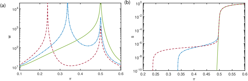
Figure 1: a) Typical size of sub-extensive connected components $w$. b) The fraction of nodes in the giant component, $s$. The solid lines correspond to uncorrected networks with $t=0$, dash-dot lines to $t=0.5$, and dashed lines to $t=1$.

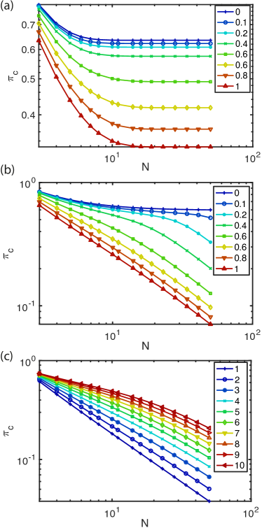
Figure 2: Critical percolation threshold $\pi_{c}$ plotted versus the maximum degree $N$ for: 1) exponential degree distribution with parameter $t$ as indicated in the legend. 2) degree distribution with tail exponent $\tau=2.5,$ and parameter $t$ as indicated in the legend. 3) degree distribution with tail exponent $\tau$ as indicated in the legend and $t=0.9$.

4 Discussion and conclusions

In this work instead of proposing yet another new model for complex networks we draw the attention to the fact that they can be treated as special cases of coloured random graphs, enabling the collection of many of the existing models under one umbrella. By using this framework, we derive several results for networks defined by their join degree-degree distributions, namely: percolation threshold (16), the size of the giant component (10), and typical size of the sub-extensive connected components (11). In this section we provide several examples where the link with coloured random graphs reveals unexpected qualitative phenomena in the behaviour of degree-degree correlated networks during random removal of edges.

4.1 Degenerate percolation transitions

Consider the degree-degree distribution given by

$$e_{j,k}=(1-t)f(j)f(k)+t\delta_{j,k}f(j),$$ (18)

where

$$f(k)=(1-\varepsilon)\delta_{k,3}+\varepsilon\delta_{k,9}.$$ (19)

with $\varepsilon=10^{-5}$. Clearly $t>0$ implies dependency between join degrees, with extreme case $t=1$ signifies that the network is composed of multiple disjoint regular graphs. The parameter $\varepsilon$ is small enough not to induce large changes in the size of the giant component, see Figure 1b. However, in the correlated case, when $t$ is close to 1, we observe two substantial peaks in the typical sizes of the sub-extensive connected components, while in the uncorrelated case, when $t$ is close to zero, there is only one peak, see Figure 1a. Note that the degree distribution is not affected by the value of the coupling parameter $t$ and is bimodal in all three cases studied in Figure 1. For all $t,$ there is only one singularity, of the type $O(\frac{1}{\pi-\pi_{c}})$, while the second peak is bounded. The example illustrates that in networks with degree dependencies, small functional perturbations to the degree distribution may cause large changes in the sizes of connected components.

4.2 Superrobust networks

Here we consider a joint degree-degree distribution (18) where, as before, parameter $t$ controls degree dependence. We analyse two functional forms of $f_{k}$: exponential distribution

$$f_{k}=C_{1}e^{-k}$$

and distribution with a heavy tail

$$f_{k}=C_{2}k^{-(\tau+1)},$$

where constants $C_{1}$ and $C_{2}$ provide normalisation. In both cases, we exclude isolated nodes, $f_{0}:=0,$ and isolated doublets $e_{1,1}:=0$. Figure 2a shows that in the exponential case, percolation threshold $\pi_{c}$ converges to a constant as maximum degree $N$ increases. Here stronger coupling $t$ corresponds to smaller values of the threshold. This is in contrast with Figure 2 b and c where $\pi_{c}$ is calculated for degree distribution with a heavy tail, showing a steady decrease of $\pi_{c}$ with increasing maximum degree $N$. This tendency is maintained across different tail exponents and values of coupling constant $t$. To date, vanishing percolation threshold has been reported only for networks with diverging second moment of the degree distribution, that is $\tau\leq 2$, a property which is also frequently inherited by the spreading processes on such networks [26]. This example indicates that networks with degree-degree dependencies may feature a vanishing percolation threshold even when the second moment of the degree distribution is finite and therefore the nodes degrees are more homogeneously distributed featuring less pronounced hubs. A direct implication of this observation is that it indicates a way to construct networks with zero percolation threshold that nevertheless do not feature strong degree heterogeneity, and therefore, are robust to random and hub-biased failures [27]. Zero percolation threshold also implies that some spreading processes that have been mapped to percolation, such as susceptible-infected-recovered model with instantaneous transmissions, will feature no epidemic threshold on much wider range of networks that was previously believed [26].

Acknowledgements

SB acknowledges kind hospitably of the Centre for Complex Systems Studies at Utrecht and the support from the Swaantje Mondt PhD Travel Fund. GP was partially supported by the Hungarian National Research, Development and Innovation Office (grants no. K128780, NVKP_16-1-2016-0004) and the Research Excellence Programme of the Ministry for Innovation and Technology in Hungary, within the framework of the Digital Biomarker thematic programme of the Semmelweis University.

References

- [1] Mark EJ Newman. The structure and function of complex networks. SIAM review, 45(2):167–256, 2003.
- [2] Nelly Litvak and Remco van der Hofstad. Uncovering disassortativity in large scale-free networks. Phys. Rev. E, 87:022801, Feb 2013.
- [3] Ernesto Estrada. Combinatorial study of degree assortativity in networks. Physical review E, 84(4):047101, 2011.
- [4] Mark EJ Newman. Assortative mixing in networks. Physical review letters, 89(20):208701, 2002.
- [5] Lia Papadopoulos, Mason A Porter, Karen E Daniels, and Danielle S Bassett. Network analysis of particles and grains. Journal of Complex Networks, 6(4):485–565, 2018.
- [6] Ariana Torres-Knoop, Ivan Kryven, Verena Schamboeck, and Piet D Iedema. Modeling the free-radical polymerization of hexanediol diacrylate (hdda): a molecular dynamics and graph theory approach. Soft matter, 14(17):3404–3414, 2018.
- [7] Mariana Olvera-Cravioto. Pagerank’s behavior under degree-degree correlations. arXiv preprint arXiv:1909.09744, 2019.
- [8] RJ Mondragón. estimating degree–degree correlation and network cores from the connectivity of high–degree nodes in complex networks. Scientific Reports, 10(1):1–24, 2020.
- [9] Sara Teller, Clara Granell, Manlio De Domenico, Jordi Soriano, Sergio Gómez, and Alex Arenas. Emergence of assortative mixing between clusters of cultured neurons. PLoS Comput Biol, 10(9):e1003796, 2014.
- [10] Marián Boguá, Romualdo Pastor-Satorras, and Alessandro Vespignani. Epidemic spreading in complex networks with degree correlations. In Statistical mechanics of complex networks, pages 127–147. Springer, 2003.
- [11] Duncan J Watts and Steven H Strogatz. Collective dynamics of ‘small-world’networks. nature, 393(6684):440–442, 1998.
- [12] Gergely Palla, Imre Derényi, Illés Farkas, and Tamás Vicsek. Uncovering the overlapping community structure of complex networks in nature and society. nature, 435(7043):814–818, 2005.
- [13] Mikko Kivelä, Alex Arenas, Marc Barthelemy, James P Gleeson, Yamir Moreno, and Mason A Porter. Multilayer networks. Journal of complex networks, 2(3):203–271, 2014.
- [14] M Angeles Serrano, Dmitri Krioukov, and Marián Boguná. Self-similarity of complex networks and hidden metric spaces. Physical review letters, 100(7):078701, 2008.
- [15] Santo Fortunato. Community detection in graphs. Physics reports, 486(3-5):75–174, 2010.
- [16] Ivan Kryven. Bond percolation in coloured and multiplex networks. Nature communications, 10(1):1–16, 2019.
- [17] Verena Schamboeck, Ivan Kryven, and Piet D. Iedema. Effect of volume growth on the percolation threshold in random directed acyclic graphs with a given degree distribution. Phys. Rev. E, 101:012303, Jan 2020.
- [18] Ivan Kryven. Emergence of the giant weak component in directed random graphs with arbitrary degree distributions. Phys. Rev. E, 94:012315, Jul 2016.
- [19] Ivan Kryven. Finite connected components in infinite directed and multiplex networks with arbitrary degree distributions. Physical Review E, 96(5):052304, 2017.
- [20] Verena Schamboeck, Piet D Iedema, and Ivan Kryven. Dynamic networks that drive the process of irreversible step-growth polymerization. Scientific reports, 9(1):1–18, 2019.
- [21] Ginestra Bianconi, Ivan Kryven, and Robert M. Ziff. Percolation on branching simplicial and cell complexes and its relation to interdependent percolation. Phys. Rev. E, 100:062311, Dec 2019.
- [22] Alexander V Goltsev, Sergey N Dorogovtsev, and José FF Mendes. Percolation on correlated networks. Physical Review E, 78(5):051105, 2008.
- [23] Marián Boguná and Romualdo Pastor-Satorras. Epidemic spreading in correlated complex networks. Physical Review E, 66(4):047104, 2002.
- [24] V. Schamboeck, P.D. Iedema, and I. Kryven. Coloured random graphs explain the structure and dynamics of cross-linked polymer networks. Unpublished, 2020.
- [25] Clara Stegehuis. Degree correlations in scale-free random graph models. Journal of Applied Probability, 56(3):672–700, 2019.
- [26] Marián Boguná, Romualdo Pastor-Satorras, and Alessandro Vespignani. Absence of epidemic threshold in scale-free networks with degree correlations. Physical review letters, 90(2):028701, 2003.
- [27] Shuai Shao, Xuqing Huang, H Eugene Stanley, and Shlomo Havlin. Percolation of localized attack on complex networks. New Journal of Physics, 17(2):023049, 2015.