Wigner and Wishart Ensembles for graphical models

Abstract.

Vinberg cones and the ambient vector spaces are important in modern statistics of sparse models and of graphical models. The aim of this paper is to study eigenvalue distributions of Gaussian, Wigner and covariance matrices related to growing Vinberg matrices, corresponding to growing daisy graphs. For Gaussian or Wigner ensembles, we give an explicit formula for the limiting distribution. For Wishart ensembles defined naturally on Vinberg cones, their limiting Stieltjes transforms, support and atom at 0 are described explicitly in terms of the Lambert-Tsallis functions, which are defined by using the Tsallis $q$-exponential functions.

1. Introduction

This paper is a first step towards studying high-dimensional asymptotics of eigenvalue distributions of Gaussian and covariance matrices related to growing statistical graphical models.

Graphical models provide one of the most powerful methods of unsupervised learning and sparse modelization of modern Data Science and high dimensional statistics (cf. Lauritzen [1996], Maathuis et al. [2018]). Mathematical bases of Wishart distributions on matrix cones related to decomposable and homogeneous graphs considered in this paper were laid down by Lauritzen [1996], Letac and Massam [2007], Ishi [2014], Graczyk and Ishi [2014].

Asymptotics of empirical eigenvalue distributions are a classical topic of the random matrix theory (RMT). There are numerous interactions of RMT with important areas of modern multivariate statistics: high dimensional statistical inference, estimation of large covariance matrices, principal component analysis (PCA), time series and many others, see the review papers by Diaconis [2003, Section 2], Johnstone [2007], Paul and Aue [2014], Bun et al. [2017], the book of Yao et al. [2015] and the references therein. RMT is also used in signal processing (including MIMO) and compressed sensing (see Hastie et al. [2015, Chapter 10], for example) in the restricted isometry property (RIP) introduced by Candès and Tao [2005]. Fujikoshi and Sakurai [2016] and Bai et al. [2018] used RMT methods to study consistency of the criteria AIC and BIC in estimation of the number of components in PCA. Distribution of the largest eigenvalue of a Wishart matrix was studied in Takayama et al. [2020].

High-dimensional spectral asymptotics for graphical models seem to have never been studied before and we are convinced that our results will be useful in modern multivariate statistical analysis in the context of graphical models. In this paper, we concentrate on proving fundamental theorems of RMT, the Wigner and Marchenko-Pastur type limit theorems for considered graphical models. We expect to study statistical applications to estimation of large covariance matrices, the number of significative PCA factors and asymptotics of the largest eigenvalue of a sparse Wishart matrix in our subsequent researches.

Growing daisy graphs are among the most natural classes of graphical models. Vinberg matrices are the symmetric matrices corresponding to the growing daisy graphs. Covariance matrices are defined naturally on them by a quadratic construction (see Section 2.4), thanks to quadratic triangular group actions on positive definite Vinberg matrices (cf. Section 2.2).

In Sections 3 and 4, we provide a complete study of limiting eigenvalue distributions related to Vinberg matrices. The main results are contained in Theorem 3.1 for the Wigner Ensembles and in Theorem 4.8 and Corollaries 4.9, 4.11 and 4.14 for the Wishart Ensembles of Vinberg matrices. We are able to treat both real and complex matrix ensembles, but in view of statistical applications, we focus on real random matrices.

As a special case of Corollary  4.9, we provide an elementary and short proof of a result of Dykema and Haagerup [2004, §8] on the asymptotic empirical eigenvalue distribution $\mu_{0}$ for the covariance of the triangular real Gaussian ensemble. The proof in Dykema and Haagerup [2004] is based on the theory of free probability with involved calculations, and the Stieltjes transform $S_{0}(z)$ is given implicitly by determining all the moments of $\mu_{0}$. Later,  Cheliotis [2018] mentioned that $S_{0}(z)$ can be expressed in terms of the Lambert $W$ function.

Our paper contributes to the study of triangular random matrices initiated by Dykema and Haagerup [2004] and continued in Cheliotis [2018], also in the framework of the theory of Muttalib-Borodin biorthogonal ensembles (see Borodin [1999], Muttalib [1995], Forrester [2010], Forrester and Wang [2017]). This is a part of recent developments in the theory of singular values of non-symmetric random matrices (see the survey by Chafaï [2009]). In contrast to Cheliotis [2018], we do not dispose of an explicit formula for the joint eigenvalue density.

The analysis, probability and statistics on homogeneous cones develops intensely in recent years (Andersson and Wojnar [2004], Graczyk and Ishi [2014], Graczyk et al. [2019], Ishi [2014, 2016], Letac and Massam [2007], Yamasaki and Nomura [2015], Nakashima [2020]), and Vinberg cones and dual Vinberg cones are basic examples of homogeneous cones (see Section 2.2). Our results are a first contribution to the RMT on homogeneous cones.

The main method used in our paper is the variance profile method for Gaussian and Wigner matrix ensembles, presented in Section 2.5. It was applied first in Shlyakhtenko [1996] in the Gaussian case and developed in Anderson and Zeitouni [2006] in the Wigner case. We use the recent approach of Bordenave [2019]. In Theorem 2.3 we slightly strengthen for our needs the main variance profile result of Bordenave [2019]. Theorem 2.3 will be useful for studying of eigenvalue distributions related to general graphical models.

Note that the variance profile methods were also developed directly for Wishart ensembles by Hachem at al. [2005, 2006, 2007], Hachem et al. [2008] (cf. Remark 4.16). The variance profile methods are related to operator-valued free probability theory (Mingo and Speicher [2017, Chapter 9]).

Our expression of a limiting Stieltjes transform for Wishart Ensembles of Vinberg matrices, is based on the introduction of Lambert-Tsallis functions $W_{\kappa,\gamma}$, see Section 4.1. The Lambert-Tsallis functions are defined by using Tsallis $q$-exponential functions, now actively studied in Information Geometry (cf. Amari and Ohara [2011], Zhang et al. [2018]).

Outlines of all proofs are given. Technical details are omitted and can be viewed in Supplementary material available from the editor of the journal.

Simulations of histograms of eigenvalues of Vinberg matrices are illustrated by Figures 7-7 in the Wigner case and by Figures 12-12 in the Wishart case.

2. Preliminaries

We begin this paper with recalling the definition of the empirical eigenvalue distribution of a symmetric matrix. Let $X\in\mathrm{Sym}(n,\mathbb{R})$ be a symmetric matrix and let $\lambda_{1}(X)\geq\cdots\geq\lambda_{n}(X)$ be the ordered eigenvalues of $X$ with counting multiplicities. Denote by $\delta_{a}$ the Dirac measure at $a$. Then, the empirical eigenvalue distribution $\mu_{X}$ of $X$ is defined by $\mu_{X}=\frac{1}{n}\sum_{i=1}^{n}\delta_{\lambda_{i}(X)}.$

If $\{X_{n}\}_{n=1}^{\infty}$ $(X_{n}\in\mathrm{Sym}(n;\,\mathbb{R}))$ is a sequence of Gaussian, Wigner or Wishart matrices, then it is well known that there exists a limit $\mu$ of $\mu_{X_{n}}$ as $n\to\infty$, and the sequence of random measures $\mu_{X_{n}}$ converges almost surely weakly to the semi-circle law or the Marchenko-Pastur law, respectively (see for example Bai and Silverstein [2010], Bordenave [2019]). The limits $\mu$ of $\mu_{X_{n}}$, in the almost sure weak sense, are said to be the “limiting eigenvalue distributions $\mu$ of $X_{n}$.” For simplicity, we will say “i.i.d. matrices” instead of “matrices with independent and identically distributed non-null terms”.

2.1. Basics on statistical graphical models

Let $G$ be a graph with vertices $V=\{1,2,\ldots,n\}$ and edges $E$. We say that a statistical character $\mathcal{X}=(X_{1},\ldots,X_{n})$ has the dependence graph $G$ when each conditional independence of marginals $X_{i}$ and $X_{j}$ with respect to remaining variables corresponds to the absence of the edge $\{i,j\}$ in $E$. Thus the dependence graph $G$ is a tool of encoding of the conditional independence of marginals of ${\mathcal{X}}$. We say that ${\mathcal{X}}$ belongs to the graphical model governed by $G$.

Let $\mathcal{U}_{G}$ be the subspace of $\mathrm{Sym}(n,\mathbb{R})$ containing matrices with $u_{ij}=0$ if the edge $\{i,j\}\not\in E$. Cones $P_{G}=\mathrm{Sym}(n,\mathbb{R})^{+}\cap\mathcal{U}_{G}$ and their dual cones $Q_{G}$ are basic objects of graphical model theory. Actually, a Gaussian $n$-dimensional model $N(m,\Sigma)$ is governed by the graph $G$ if and only if the inverse covariance matrix $\Sigma^{-1}\in P_{G}$ (cf. Lauritzen [1996]).

Figure 1. Daisy Graph

An important class of graphical models, called daisy graphs, is defined as follows. Let $a+b=n$ and let $D(a,b)$ be a graph with vertices $V=\{1,\dots,n\}$, such that the first $a$ elements form a complete graph and the latter $b$ elements are satellites (petals) of the complete graph, that is, each satellite connects to all elements in the complete graph and does not connect to the other satellites (see Figure 1). The double circle around the vertex $a_{n}$ in Figure 1 indicates the complete graph with $a_{n}$ vertices.

In high dimensional statistics, it is essential to let the number of observed characters $n$ tend to infinity. From the graphical model theory point of view, the pattern of the growing graphs $G_{n}$ and of the corresponding cones $P_{G_{n}}$ should remain the same. This requirement is met by growing daisy graphs $D(a_{n},b_{n})$ for non-decreasing sequences of positive integers $\{a_{n}\}_{n=1}^{\infty}$ and $\{b_{n}\}_{n=1}^{\infty}$ such that $a_{n}+b_{n}=n$.

2.2. Generalized dual Vinberg cones and Vinberg matrices

Let $\{a_{n}\}_{n=1}^{\infty}$ and $\{b_{n}\}_{n=1}^{\infty}$ be non-decreasing sequences of positive integers such that $a_{n}+b_{n}=n$ and the ratio $a_{n}/n$ converges to $c\in[0,1]$. Let $G_{n}=D(a_{n},b_{n})$ be the corresponding daisy graph. Then, the corresponding matrix space $\mathcal{U}_{n}$ of the graph $G_{n}$ is a subspace of $\mathrm{Sym}(n,\mathbb{R})$ defined by

$$\mathcal{U}_{n}:=\left\{{U}=\begin{pmatrix}x&y\\ {}^{t}y&d\end{pmatrix};\;\begin{array}[]{l}x\in\mathrm{Sym}(a_{n},\mathbb{R}),\,y\in\mathrm{Mat}(a_{n}\times b_{n},\mathbb{R}),\\ \text{$d$ is a diagonal matrix of size $b_{n}$}\end{array}\right\},$$

and we set

$$P_{n}:=P_{G_{n}}=\mathcal{U}_{n}\cap\mathrm{Sym}(n,\mathbb{R})^{+}.$$

Then, $P_{n}$ is an open convex cone in $P_{G_{n}}$. Moreover, the cone $P_{n}$ admits a transitive group action, i.e. $P_{n}$ is a homogeneous cone, since the following triangular group

$$H_{n}:=\left\{h=\begin{pmatrix}h_{1}&y\\ 0&d\end{pmatrix}\in GL(n,\mathbb{R});\;\begin{array}[]{l}h_{1}\in GL(a_{n},\mathbb{R})\text{ is upper triangular},\\ y\in\mathrm{Mat}(a_{n}\times b_{n};\,\mathbb{R}),\\ d\colon\text{diagonal of size }b_{n}\end{array}\right\}$$

acts on $P_{n}$ transitively by the quadratic action $\rho(h){U}:=h{U}{}^{\,t\!}h$ for $h\in H_{n}$ and ${U}\in P_{n}$. This is easily verified by using the Cholesky decomposition (cf. Ishi [2016, p. 3]). For definition and basic properties of homogeneous cones, see Vinberg [1963], Ishi [2014].

If $n=3$ and $(a_{n},b_{n})=(1,2)$, then $P_{3}$ is the dual Vinberg cone (see Example 2.1) so that, in this paper, we call $P_{n}$ a generalized dual Vinberg cone and elements $U\in\mathcal{U}_{n}$ Vinberg matrices. Vinberg cones form an important class of matrix cones related to graphical models (cf. Section 2.1). On the other hand, if we set $a_{n}=n-1$ and $b_{n}=1$, then $\mathcal{U}_{n}$ is the space $\mathrm{Sym}(n,\mathbb{R})$ of symmetric matrices of size $n$, and hence our discussion covers the classical results. In what follows, we introduce two kinds of random matrices related to the homogeneous cones $P_{n}$, that is, Gaussian and Wigner matrices and Wishart quadratic (covariance) matrices.

2.3. Gaussian and Wigner matrices in $\mathcal{U}_{n}$

Analogously to the classical Wigner matrices, we say that $U_{n}=(u_{ij})\in\mathcal{U}_{n}$ is a Wigner random matrix if

$$\left\{\rule{0.0pt}{40.0pt}\right. \bullet (u_{ii}) (u_{ij})_{i<j} \bullet u_{ii} v^{\prime} M_{4}^{\prime} \bullet u_{ij} i<j v {M_{4}}$$ the diagonal terms are independent of the off-diagonal terms , the diagonal ’s are centered i.i.d. variables with variance and fourth moment , the non-nul off-diagonal ’s, , are centered i.i.d. variables with variance and fourth moment , (2.1)

where $v,v^{\prime},M_{4},M_{4}^{\prime}$ are fixed positive real numbers. If the non-nul terms $u_{ij}$ are Gaussian, with $\nu=1$ and $\nu^{\prime}=2$, the matrices $U_{n}$ form a Gaussian Orthogonal Ensemble of Vinberg matrices.

In Section 3, we consider empirical eigenvalue distributions of rescaled Wigner matrices $U_{n}/\sqrt{n}\in\mathcal{U}_{n}$.

2.4. Quadratic construction of Wishart (covariance) matrices in $\mathcal{U}_{n}$

Recall that Wishart matrices are constructed quadratically both in Random Matrix Theory and in statistics. In this section we define, by a quadratic construction, Wishart (covariance) matrices in $\mathcal{U}_{n}$.

We first recall the notion of a direct sum of quadratic maps. Let $Q_{i}\colon\mathbb{R}^{m_{i}}\to\mathbb{R}^{m}$ $(i=1,\dots,k)$ be quadratic maps. Then, the direct sum $Q_{1}\oplus\cdots\oplus Q_{k}$ is an $\mathbb{R}^{m}$-valued quadratic map on $\mathbb{R}^{m_{1}}\oplus\cdots\oplus\mathbb{R}^{m_{k}}$ given by

$$Q(x):=Q_{1}(x_{1})+\cdots+Q_{k}(x_{k})\quad\text{where}\quad x=\sum_{i=1}^{k}x_{i}\quad\bigl{(}x_{i}\in\mathbb{R}^{m_{i}}\bigr{)}.$$

If $Q_{1}=\cdots=Q_{k}$, then the direct sum $Q$ is denoted by $Q_{1}^{\oplus k}$. As showed in Graczyk and Ishi [2014], any homogeneous cone $\Omega$ admits a canonical family of the so-called basic quadratic maps $q_{j}$ ($j=1,\ldots,r$) defined for each $j$ on a suitable finite dimensional vector space $E_{j}$ and with values in the closure $\overline{\Omega}$ of $\Omega$. The number $r$ is called the rank of $\Omega$ and $r=n$ for the cones $\mathcal{U}_{n}$. Using the basic quadratic maps $q_{j}$, one constructs quadratic maps $Q_{\underline{k}}$ for $\underline{k}\in\mathbb{Z}^{r}_{\geq 0}$ by

$$Q_{\underline{k}}:=q_{1}^{\oplus k_{1}}\oplus\cdots\oplus q_{r}^{\oplus k_{r}},$$

defined on $E_{\underline{k}}:=E_{1}^{\oplus k_{1}}\oplus\cdots\oplus E_{r}^{\oplus k_{r}}$. The maps $Q_{\underline{k}}$ are $\Omega$-positive, i.e. if $\xi\in E_{\underline{k}}\setminus\{\boldsymbol{0}\}$, then $Q_{\underline{k}}(\xi)\in\overline{\Omega}\setminus\{\boldsymbol{0}\}$.

In our case $\Omega=P_{n}$, the basic quadratic maps are given as follows (cf. Graczyk and Ishi [2014]). For $j=1,\dots,n$, define $E_{j}\subset\mathbb{R}^{n}$ by

$$\begin{array}[]{l}E_{j}=\left\{\begin{pmatrix}\boldsymbol{\xi}\\ \boldsymbol{0}\end{pmatrix}\in\mathbb{R}^{n};\;\boldsymbol{\xi}\in\mathbb{R}^{j}\right\}\quad(j\leq a_{n}),\\[8.00003pt] E_{j}=\left\{\begin{pmatrix}\boldsymbol{\xi}\\ \boldsymbol{0}\end{pmatrix}+\xi^{\prime}\boldsymbol{e}_{j}\in\mathbb{R}^{n};\;\boldsymbol{\xi}\in\mathbb{R}^{a_{n}},\ \xi^{\prime}\in\mathbb{R}\right\}\quad(j>a_{n}),\end{array}$$

where $\boldsymbol{e}_{i}$ $(i=1,\dots,n)$ is the vector in $\mathbb{R}^{n}$ having $1$ on the $i$-th position and zeros elsewhere. We note that each $E_{j}$ corresponds to the $j$-th column of the Lie algebra $\mathfrak{h}_{n}$ of $H_{n}$, that is, we have $\mathfrak{h}_{n}=\left\{H=(\boldsymbol{\xi}_{1},\dots,\boldsymbol{\xi}_{n});\;\boldsymbol{\xi}_{j}\in E_{j}\right\}$. Then, the basic quadratic maps $q_{j}\colon E_{j}\to\mathcal{U}_{n}$ of the cone $P_{n}$ are defined by

$$q_{j}(\boldsymbol{\xi}_{j}):=\boldsymbol{\xi}_{j}{}^{\,t\!}\boldsymbol{\xi}_{j}\in\mathcal{U}_{n}\quad(\boldsymbol{\xi}_{j}\in E_{j}).$$

Let $\underline{k}\in\mathbb{Z}_{\geq 0}^{n}$. Then, $E_{\underline{k}}$ can be viewed as a subspace of $\mathrm{Mat}(n\times(k_{1}+\cdots+k_{n});\,\mathbb{R})$. In fact, we have

$$\begin{array}[]{l}\displaystyle E_{\underline{k}}=\left\{\eta=\Bigl{(}\overbrace{\boldsymbol{\xi}_{1}^{(1)},\dots,\boldsymbol{\xi}_{1}^{(k_{1})}}^{k_{1}},\boldsymbol{\xi}_{2}^{(1)},\dots,\boldsymbol{\xi}_{n-1}^{(k_{n-1})},\overbrace{\boldsymbol{\xi}_{n}^{(1)},\dots,\boldsymbol{\xi}_{n}^{(k_{n})}}^{k_{n}}\Bigr{)};\;\begin{array}[]{l}\boldsymbol{\xi}_{j}^{(i)}\in E_{j},\\ j=1,\dots,n,\\ i=1,\dots,k_{j}\end{array}\right\}\\[10.00002pt] \hfill{}\subset\mathrm{Mat}(n\times(k_{1}+\cdots+k_{n});\,\mathbb{R}),\end{array}$$

and then $Q_{\underline{k}}(\eta)=\eta{}^{\,t\!}\eta$ for $\eta\in E_{\underline{k}}$.

When $\eta\in E_{\underline{k}}$ is an i.i.d. random matrix whose non-null terms have the normal law $N(0,v)$, the law of $Q_{\underline{k}}(\eta)$ is a Wishart law $\gamma_{Q_{\underline{k}},1/(2v){\rm Id}_{n}}$ on the cone $P_{n}$. For the definition of all Wishart laws on the cone $P_{n}$, see Graczyk and Ishi [2014]. More generally, in this paper, we consider eigenvalue distributions of rescaled matrix $Q_{\underline{k}}(\eta)/n$ under the assumption that $\eta\in E_{\underline{k}}$ is a centered rectangular i.i.d. matrix whose non-null terms have variance $v$ and finite fourth moments $M_{4}$.

We consider two-dimensional multiparameters $\underline{k}=\underline{k}(n)\in\mathbb{Z}_{\geq 0}^{n}$ of the form

$$\underline{k}=m_{1}(1,\dots,1)+m_{2}(\,\overbrace{0,\dots,0}^{a_{n}},\overbrace{1,\dots,1}^{b_{n}}\,)\quad(m_{1},m_{2}\in\mathbb{Z}_{\geq 0}).$$ (2.2)

Example 2.1.

Let $n=3$, $a_{3}=1$ and $b_{3}=2$. In this case, $P_{3}$ is the dual Vinberg cone (cf. Vinberg [1963, p. 397], Ishi [2001, §5.2]):

$$P_{3}=\left\{x=\begin{pmatrix}x_{11}&x_{12}&x_{13}\\ x_{12}&x_{22}&0\\ x_{13}&0&x_{33}\end{pmatrix};\;\textrm{$x$ is positive definite}\right\}.$$

Consider $m_{1}=m_{2}=1$, so $\underline{k}=(1,2,2)$. Then $E_{\underline{k}}=E_{(1,2,2)}$ can be written as

$$E_{(1,2,2)}=\left\{\eta=\begin{pmatrix}x&y_{11}&y_{12}&z_{11}&z_{12}\\ 0&y_{21}&y_{22}&0&0\\ 0&0&0&z_{21}&z_{22}\end{pmatrix};\;x,y_{ij},z_{ij}\in\mathbb{R}\right\},$$

and $Q_{(1,2,2)}(\eta)=\eta{}^{\,t\!}\eta$ is given as

$$Q_{(1,2,2)}(\eta)=\begin{pmatrix}x^{2}+y_{11}^{2}+y_{12}^{2}+z_{11}^{2}+z_{12}^{2}&y_{11}y_{21}+y_{12}y_{22}&z_{11}z_{21}+z_{12}z_{22}\\ y_{11}y_{21}+y_{12}y_{22}&y_{21}^{2}+y_{22}^{2}&0\\ z_{11}z_{21}+z_{12}z_{22}&0&z_{21}^{2}+z_{22}^{2}\end{pmatrix}.$$

If $x,y_{ij},z_{ij}$ are $N(0,v)$ i.i.d. Gaussian variables, the random matrix $Q_{(1,2,2)}(\eta)$ has a Wishart law on $P_{3}$.

The form (2.2) of the Wishart multiparameter $\underline{k}$ englobes and generalizes the following cases. In both cases, with rescaling $1/n$, the limiting eigenvalue distribution is known.

1. The classical Wishart Ensemble $M\,^{t}M$ on $\mathrm{Sym}(n,\mathbb{R})^{+}$, where $M=M_{n\times N}$ is an i.i.d. matrix with finite fourth moment ${M_{4}}$, with parameter $C:=\lim_{n}\frac{N}{n}>0$ (see Anderson et.al. [2010], Faraut [2014]) for $(a_{n},b_{n})=(n-1,1)$, $m_{1}=0$ and $m_{2}\sim Cn$. The limiting eigenvalue distribution is the Marchenko-Pastur law $\mu_{C}$ with parameter $C$, i.e. denoting $a=\bigl{(}\sqrt{C}-1\bigr{)}^{2},b=\bigl{(}\sqrt{C}+1\bigr{)}^{2}$ and $[x]_{+}:=\max(x,0)$ $(x\in\mathbb{R})$,

   $$\mu_{C}=[1-C]_{+}\delta_{0}+\frac{\sqrt{(t-a)(b-t)}}{2\pi t}\,\chi_{[a,b]}(t)dt.$$

2. The Wishart Ensemble related to the Triangular Gaussian Ensemble
   (Dykema and Haagerup [2004], Cheliotis [2018]) for $(a_{n},b_{n})=(n-1,1)$, $m_{1}=1$ and $m_{2}=0$. When $v=1$, the limiting eigenvalue distribution, which we call the Dykema-Haagerup measure $\chi_{1}$, is absolutely continuous with respect to Lebesgue measure and has support equal to the interval $[0,e]$. Its density function $\phi$ is defined on the interval $(0,e]$ by the implicit formula (Dykema and Haagerup [2004, Theorem 8.9])

   $$\phi\left(\frac{\sin x}{x}\,\exp(x\cot x)\right)=\frac{1}{\pi}\sin x\exp(-x\cot x)\qquad(0\leq x<\pi),$$ (2.3)

   with $\phi(0+)=\infty$ and $\phi(e)=0$. For $v\not=1$, the limiting measure $\chi_{v}$ has density $\phi({y}/{v})/v$ on the segment $(0,ve]$.

2.5. Resolvent method for Wigner ensembles with a variance profile $\sigma$

Let $\mathbb{C}^{+}$ denote the upper half plane in $\mathbb{C}$. In this paper, the Stieltjes transform $S(z)=S_{\mu}(z)$ of a probability measure $\mu$ on $\mathbb{R}$ is defined to be

$$S(z)=\int_{\mathbb{R}}\frac{\mu(dt)}{t-z}\quad(z\in\mathbb{C}^{+}).$$

In the sequel, we will need the following properties of the Stieltjes transform, which are not difficult to prove.

Proposition 2.2.

1. Suppose that $s(z)$ is the Stieltjes transform of a finite measure $\nu$ on $\mathbb{R}$. If for all $x\in\mathbb{R}$ it holds

$$\lim_{y\to 0+}\mathrm{Im}\,s(x+iy)=0$$

then $s(z)\equiv 0$ and $\nu$ is a null measure ($\nu(B)=0$ for any Borel set $B$).
2. Suppose $f\geq 0$ and $f\in L^{1}(\mathbb{R})$. Let $s(z)$ be the Stieltjes transform of $f$. If $f$ is continuous at $x$ then

$$\lim_{y\to 0+}\frac{1}{\pi}\mathrm{Im}\,s(x+iy)=f(x).$$ (2.4)

If $f$ is continuous on an interval $[a,b]$, $a<b$, the convergence (2.4) is uniform for $x\in[a,b]$.

Recall that if $\mu$ is a probabilistic measure on $\mathbb{R}$, with Stieltjes transform $s(z)$ and the absolutely continuous part of $\mu$ has density $f$, then (2.4) holds for almost all $x$ (Lemma 3.2 (iii) of Bordenave [2019]).

We present now the following, slightly strengthened result from the Lecture Notes of Bordenave [2019, §3.2], that will be a main tool of proofs in this paper.

Let $\sigma\colon[0,1]\times[0,1]\to[0,\infty)$ be a bounded Borel measurable symmetric function. For each integer $n$, we partition the interval $[0,1]$ into $n$ equal intervals $J_{i},i=1,\ldots,n$. Put $Q_{ij}:=J_{i}\times J_{j}$, which is a partition of $[0,1]\times[0,1]$. We assume that $Y_{ij}$ $(i\leq j)$ are independent centered real variables, defined on a common probability space, with variance

$$\mathbb{E}Y_{ij}^{2}=\frac{1}{n}\left(\int_{Q_{ij}}\frac{\sigma(x,y)}{|Q_{ij}|}\,dx\,dy+\delta_{ij}(n)\right),$$ (2.5)

for a sequence $\delta_{ij}(n)$. We note that the law of $Y_{ij}$ depends on $n$. We set $Y_{ji}:=Y_{ij}$ and we consider the symmetric matrix $Y_{n}:=(Y_{ij})_{1\leq i,j\leq n}.$ We note that, if $\sigma$ is continuous, then, up to a perturbation $\delta_{ij}(n)$, the variance of $\sqrt{n}Y_{ij}$ is approximatively ${\sigma(i/n,j/n)}$, and hence we call $\sigma$ a variance profile in this paper.

Theorem 2.3.

Let $\delta_{0}(n):=\displaystyle\frac{1}{n^{2}}\sum_{i,j\leq n}|\delta_{ij}(n)|$. Assume (2.5) and suppose that

$$\lim_{n}\delta_{0}(n)=0\quad\text{and}\quad\max_{i,j\leq n}\frac{\mathbb{E}(Y_{ij}^{4})}{n(\mathbb{E}Y_{ij}^{2})^{2}}=o(1)\quad(Y_{ij}\not=0).$$ (2.6)

Let $\mu_{Y_{n}}$ be the empirical eigenvalue distribution of $Y_{n}$. Then, there exists a probability measure $\mu_{\sigma}$ depending on $\sigma$ such that $\mu_{Y_{n}}$ converges weakly to $\mu_{\sigma}$ almost surely. The Stieltjes transform $S_{\sigma}$ of $\mu_{\sigma}$ is given as follows.
(a) For each $z$ with $\mathrm{Im}\,z>1$, there exists a unique $\mathbb{C}^{+}$-valued $L^{1}$-solution $\eta_{z}:[0,1]\mapsto\mathbb{C}^{+}$, of the equation

$$\eta_{z}(x)=-\left(z+\int_{0}^{1}\sigma(x,y)\,\eta_{z}(y)\,dy\right)^{-1}\quad(\text{for almost all $x\in[0,1]$}),$$ (2.7)

and the function $z\mapsto\eta_{z}(x)$ extends to an analytic $\mathbb{C}^{+}$-valued function on $\mathbb{C}^{+}$, for almost all $x\in[0,1]$. Then,

$$S_{\sigma}(z)=\int_{0}^{1}\eta_{z}(x)\,dx.$$

(b) The function $x\to\eta_{z}(x)$ is also a solution of (2.7) for $0<\mathrm{Im}\,z\leq 1.$

Proof.

The proof is the same as the proof of Bordenave [2019, Theorem 3.1], where a stronger assumption $|\delta_{ij}(n)|\leq\delta(n)$ is required for some sequence $\delta(n)$ going to 0. It is replaced by the first condition of (2.6). Detailed analysis of the proof of the approximate fixed point equation in Bordenave [2019, page 42] shows that the weakest assumption on the fourth moments $\mathbb{E}Y_{ij}^{4}$ ensuring the concentration of the conditional variance of $\langle Z_{i},R^{(i)}Z_{i}\rangle$ is the second condition of (2.6). The property (b) is observed in Bordenave [2019, page 39] by analiticity. ∎∎

Theorem 2.3 shows that, to each variance profile function $\sigma$, one associates uniquely a Stieltjes transform $S_{\sigma}(z)$ of a probability measure. For the correspondence between $\sigma$ and $S_{\sigma}$, the conditions (7) are not needed. We define $S_{\sigma}(z)$ as the Stieltjes transform associated to $\sigma$.

Remark 2.4.

A prototype of the variance profile method for Wigner ensembles was given by Anderson and Zeitouni [2006, Theorem 3.2]. Theorem 3.1 of Bordenave [2019] and Theorem 2.3 provide a simple general approach. Special cases of variance profile convergence results for Wigner matrices were studied before, as discussed below in (i) and (ii).

(i)

If we set $\sigma(x,y)=1$ for all $x,y$, then $\sqrt{n}Y$ is a Wigner ensemble with $v=v^{\prime}=1$. Let $S_{\mathrm{sc}}(z)$ be the Stieltjes transform of the semi-circle law on $[-2,2]$. Then, the functions $x\to\eta_{z}(x)$ do not depend on $x$ (but do on $z$) and the functional equation (2.7) gives the equation $S_{\mathrm{sc}}(z)=-(z+S_{\mathrm{sc}}(z))^{-1}$, which is well known from the detailed study of resolvent matrices (see Tao [2012, §2.4.3]).

(ii)

The paper Anderson and Zeitouni [2006] deals primarily with a variance profile $\sigma$ such that $\int\sigma(x,y)\,dy=1$ for any $x$, corresponding to a band matrix model. For band matrix ensembles, see also Erdös et al. [2012, 2012b], Nica et al. [2002], Shlyakhtenko [1996].

3. Wigner Ensembles of Vinberg Matrices

In this section, we give explicitly the limiting eigenvalue distributions $\mu$ for the scaled Wigner matrices $U_{n}\in\mathcal{U}_{n}$ defined by (2.1). Let $\chi_{I}$ denote the indicator function of a subset $I\subset\mathbb{R}$. For a real number $a$, its cubic root is denoted by $\sqrt[3]{a}\in\mathbb{R}$ and set $[\,a\,]_{+}=\max(a,0)$. We introduce two real numbers $\alpha_{c}$, $\beta_{c}$ depending on $c\in[0,1)$ by

$$\alpha_{c}=\frac{8+4c-13c^{2}-\sqrt{c(8-7c)^{3}}}{8(1-c)},\ \beta_{c}=\frac{8+4c-13c^{2}+\sqrt{c(8-7c)^{3}}}{8(1-c)}.$$ (3.8)

It is clear that $\alpha_{0}=\beta_{0}=1$, $\alpha_{c}<\beta_{c}$ and $\beta_{c}>0$ for all $c\in(0,1)$. We note that $\alpha_{1/2}=0$, $\alpha_{c}<0$ when $c>1/2$, $\lim_{c\to 1-}\alpha_{c}=-\infty$, $\lim_{c\to 1-}(1-c)\alpha_{c}=-1/4$ and $\lim_{c\to 1-}\beta_{c}=4$, so that we set $\beta_{1}=4$. It can be shown that $c\mapsto\alpha_{c}$ is strictly decreasing and $c\mapsto\beta_{c}$ is strictly increasing on $[0,1]$ (see Figure 7).

Theorem 3.1.

Let $U_{n}$ be a Wigner matrix on $\mathcal{U}_{n}$ defined by (2.1). Assume that $\lim_{n\to+\infty}a_{n}/n=c\in(0,1)$. Then, the limiting eigenvalue distribution $\mu$ of the rescaled matrices $U_{n}/\sqrt{n}$ exists and is given for $c\in(0,1)$ as

$$\mu=f_{c}(t)\,dt+[1-2c]_{+}\delta_{0}$$

with

$$f_{c}(t):=\frac{\sqrt[3]{R_{+}\left(t/\!\sqrt{v};\,c\right)}-\sqrt[3]{R_{-}\left(t/\!\sqrt{v};\,c\right)}}{2\sqrt{3}\pi\,t}\,\chi_{[\alpha_{c},\beta_{c}]}\left(\frac{t^{2}}{v}\right),$$ (3.9)

where, for $x^{2}\in[\alpha_{c},\beta_{c}]$,

$$\begin{array}[]{r@{\ }c@{\ }l}R_{\pm}(x;\,c)&:=&x^{6}-3(c+1)x^{4}+\frac{3}{2}(5c^{2}-2c+2)x^{2}+(2c-1)^{3}\\[6.00006pt] &&\qquad\pm 3c\sqrt{3-3c}\cdot x\sqrt{(x^{2}-\alpha_{c})(\beta_{c}-x^{2})}.\end{array}$$

The support of $\mu$ is given as

$$\!\mathop{\mathrm{missing}}{supp}\mu=\begin{cases}\left[\,-\sqrt{v\beta_{c}},\,-\sqrt{v\alpha_{c}}\,\right]\cup\{0\}\cup\left[\,\sqrt{v\alpha_{c}},\,\sqrt{v\beta_{c}}\,\right]&(\text{if }\ c\in(0,\frac{1}{2}))\\[10.00002pt] \left[\,-\sqrt{v\beta_{c}},\,\sqrt{v\beta_{c}}\,\right]&(\text{if }\ c\in[\tfrac{1}{2},1)).\end{cases}$$ (3.10)

If $c=0$, then $\mu=\delta_{0}$. If $c=1$, then $\mu$ is the semicircle law on $[-2\sqrt{v},2\sqrt{v}]$.

Remark 3.2.

The formula (3.9) is valid for the extreme cases $c=0$ or $c=1$. If $c=0$ then there is no density and $\mu=\delta_{0}$. If $c=1$, then it can be checked that $\sqrt[3]{R_{+}(x;\,1)}-\sqrt[3]{R_{-}(x;\,1)}=\sqrt{3}x\,\sqrt{4-x^{2}}$ so that, for $v=1$ we get the semicircle law $\mu(dt)=(1/2\pi)\sqrt{4-t^{2}}\chi_{[-2,2]}(t)dt$ of  Wigner [1955].

Sketch of the proof.

We first derive the Stieltjes transform of the limiting eigenvalue distribution by applying Theorem 2.3 to $Y_{n}=U_{n}/\sqrt{n}$. Let $U_{n}=(U_{ij})_{1\leq i,j\leq n}$, so that $Y_{ij}=(1/\sqrt{n})U_{ij}$. The variance profile is given as

$$\sigma(x,y)=\left\{\begin{array}[]{l}v\quad\text{if}\ (x,y)\in\mathcal{C},\\ 0\quad\text{otherwise,}\end{array}\right.\quad\mathcal{C}:=\left\{(x,y)\in[0,1]^{2};\;\min(x,y)\leq c\right\}.$$ (3.11)

We check easily that the conditions (2.6) are satisfied, since, by (2.1) and writing $M:=\max\{|v-v^{\prime}|,v^{\prime},v\}$, we get

$$\delta_{0}(n)\leq\frac{3M}{n}\quad\textrm{and }\quad\max_{i,j\leq n}\frac{\mathbb{E}(Y_{ij}^{4})}{n(\mathbb{E}Y_{ij}^{2})^{2}}\leq\frac{\max\{{{M_{4}},{M_{4}}^{\prime}}\}}{n\min\{v,v^{\prime}\}}.$$

Let us fix $z\in\mathbb{C}^{+}=\left\{z\in\mathbb{C};\;\mathrm{Im}\,z>0\right\}$. The functional equation (2.7) from Theorem 2.3 becomes

$$\eta_{z}(x)=\begin{cases}-\left(z+v\int_{0}^{1}\eta_{z}(y)\,dy\right)^{-1}&(x\leq c),\\[8.00003pt] -\left(z+v\int_{0}^{c}\eta_{z}(y)\,dy\right)^{-1}&(x>c).\end{cases}$$

Observe that the right-hand sides are independent of $x$. Integrating both sides of these equations, we obtain the following simultaneous equations

$$B=\frac{-c}{z+vA},\quad A-B=\frac{c-1}{z+vB},$$ (3.12)

where $A=\int_{0}^{1}\eta_{z}(x)\,dx$ and $B=\int_{0}^{c}\eta_{z}(x)\,dx$. Note that $A$ is the desired Stieltjes transform $S(z)$.

If $c=0$, then we have $A=-1/z$ so that the limiting measure is $\mu=\delta_{0}$. If $c=1$ then the equation (2.7) reduces to the equation $A=-(z+vA)^{-1}$, which corresponds to the Stieltjes transform of the semi-circular law (cf. Tao [2012, p.178]). Thus we assume $0<c<1$ in what follows.

Then, the cubic equation for $A$, resulting from (3.12) writes

$$zA^{3}+(2z^{2}+1-2c)A^{2}+(z^{2}+2-2c)zA+z^{2}-c^{2}=0$$ (3.13)

and it is an algebraic equation with polynomial coefficients. The last equation (3.13) is reduced to

$$Y^{3}+p\left(z_{v}\right)Y+q\left(z_{v}\right)=0,$$ (3.14)

where we set $z_{v}:={z}/{\sqrt{v}}$,

$$Y=Y(z):=\frac{vA}{z}+\frac{2}{3}-\frac{(2c-1)v}{3z^{2}},$$ (3.15)

and the coefficients $p,q$ are given by the following analytical rational functions on $\mathbb{C}^{*}{:=\mathbb{C}\setminus\{0\}}$

$$\begin{array}[]{l}\displaystyle p(z):=-\frac{z^{4}-2(c+1)z^{2}+(2c-1)^{2}}{3z^{4}},\\[10.00002pt] \displaystyle q(z):=-\frac{2}{27}\cdot\frac{z^{6}-3(c+1)z^{4}+\frac{3}{2}(5c^{2}-2c+2)z^{2}+(2c-1)^{3}}{z^{6}}.\end{array}$$

The discriminant of the cubic equation (3.14) is expressed by $p(z)$ and $q(z)$, using $\alpha_{c},\beta_{c}$ in (3.8), as (cf. Ronald [2004])

$$\mathop{\mathrm{missing}}{Disc}(z)=-\bigl{(}4p(z)^{3}+27q(z)^{2}\bigr{)}=\frac{4c^{2}(1-c)}{z^{10}}(z^{2}-\alpha_{c})(z^{2}-\beta_{c}).$$

Let $\mathcal{E}=\left\{z\in\mathbb{C};\;z=0\text{ or }\mathop{\mathrm{missing}}{Disc}(z_{v})=0\right\}$ be the set of exceptional points of (3.14). For $z\not\in\mathcal{E}$, the equation (3.14) has three different solutions (cf. Ronald [2004]). Cardano’s method and formula (3.15) imply that, for $z\in\mathbb{C}^{+}$

$$S(z)=\frac{z(u_{+}(z)+u_{-}(z))}{3v}-\frac{2z}{3v}+\frac{2c-1}{3z}$$ (3.16)

with $u_{\pm}(z):=\left(F_{c}(z_{v})\pm i\,D_{c}(z_{v})\right)^{\frac{1}{3}}$, $F_{c}(z):=-\frac{27}{2}q(z)$ and

$$D_{c}(z):=27\cdot\sqrt{\frac{\mathop{\mathrm{missing}}{Disc}(z)}{4\cdot 27}}=\frac{3c\sqrt{3-3c}}{z^{5}}\,\sqrt{(z^{2}-\alpha_{c})(z^{2}-\beta_{c})},$$

where convenient branches of the cube and the square roots are chosen, respectively, for $u_{\pm}(z)$ and $D_{c}(z)$ to be such that $S(z)$ is a Stieltjes transform of a probability measure. In particular, $S(z)$ is holomorphic on $\mathbb{C}^{+}$ and

$$u_{+}(z)\cdot u_{-}(z)=-3p(z),\quad\textrm{and}\quad\mathrm{Im}\,S(z)>0\quad(z\in\mathbb{C}^{+}).$$ (3.17)

Note that the branches of the roots may be different on different subregions of $\mathbb{C}^{+}$ and that $U:=(u_{+}+u_{-})/3$ is a solution of (3.14). In order to derive the limiting eigenvalue distribution $\mu$ from $S(z)$, we will need the following properties of $S(z)$. Set $\mathbb{R}^{*}:=\mathbb{R}\setminus\{0\}$.

Proposition 3.3.

The limit $\displaystyle S(x)=\lim_{y\to+0}S(x+yi)$ exists for each $x\in\mathbb{R}^{*}$. The function $S$ is continuous on $\mathbb{R}^{*}$ and $S(x)$ is a solution of (3.13) on $\mathbb{R}^{*}$.

Sketch of the proof of the proposition.

It is sufficient to prove it for a solution $U(z)$ of the reduced equation (3.14) on $\mathbb{C}^{+}$, such that $U(z)$ is holomorphic on $\mathbb{C}^{+}$. We apply Theorem X.3.7 of Palka [1991] to a convenient connected and simply connected domain $D$ avoiding the set $\mathcal{E}$. By the discussion of Ahlfors [1979, p.304], $U$ has at most an ordinary algebraic singularity at a non-zero exceptional point, so $U(z)$ is continuous on $\mathbb{R}^{*}$. ∎∎

Without loss of generality, we suppose $v=1$. We first assume that $x=0$. The detailed local analysis of (3.16) and (3.17) that we omit here, shows that

1. if $0<c<\frac{1}{2}$, then $\displaystyle\lim_{y\to+0}y\textrm{Im}\,S(yi)=1-2c$, so $\mu$ has an atom at $0$ with the mass $1-2c<1$,

2. if $c=\frac{1}{2}$, then $\displaystyle\lim_{y\to+0}\textrm{Im}\,S(yi)=+\infty,\ \lim_{y\to+0}y\textrm{Im}\,S(yi)=0$ so $\mu$ does not have an atom at $0$,

3. if $\frac{1}{2}<c<1$, then $\displaystyle\lim_{y\to+0}\textrm{Im}\,S(yi)=c(2c-1)^{-1/2}=\pi f_{c}(0)$, so $\mu$ does not have an atom at $0$.

Next we consider the case $x\neq 0$. Combining the fact that $S(z)$ is an odd function as a function on $\mathbb{C}\setminus\mathbb{R}$ by (3.16) and the property $S(\overline{z})=\overline{S(z)}$ of the Stieltjes transform, we obtain $\mathrm{Im}\,S(-x+iy)=\mathrm{Im}\,S(x+iy)$ so that $\mathrm{Im}\,S(-x)=\mathrm{Im}\,S(x)$. Thus we can assume that $x>0$.

Suppose $\mathop{\mathrm{missing}}{Disc}(x)\geq 0$. Since the coefficients $p,q$ of (3.14) are real on $\mathbb{R}^{*}$, the equation (3.14) has only real solutions (cf. Ronald [2004]). Therefore, $S(x)$ is real so that the density of $\mu$ vanishes at such points.

Next we assume that $\mathop{\mathrm{missing}}{Disc}(x)<0$. By Proposition 3.3, $S(x)$ is a solution of the cubic equation (3.13) and $U(x)=(u_{+}(x)+u_{-}(x))/3$ is a solution of the reduced equation (3.14). In particular, the formulas (3.16) and (3.17) hold for $S(x)$, with convenient choices of branches of cubic roots and square roots. Consequently, we have

$\bigl{\{}F_{c}(x)+iD_{c}(x),F_{c}(x)-iD_{c}(x)\bigr{\}}=\bigl{\{}R^{\prime}_{+}(x),\,R^{\prime}_{-}(x)\bigr{\}}$

as a set, where $R^{\prime}_{\pm}(x):=R_{\pm}(x;\,c)/x^{6}\in\mathbb{R}$. Let $\omega=e^{2i\pi/3}$ denote the cube root of $1$ with positive imaginary part. Then, (3.16) yields that the sum $u_{+}(x)+u_{-}(x)$ has the following form

$$u_{+}(x)+u_{-}(x)=\omega^{k_{+}}\sqrt[3]{R^{\prime}_{+}(x)}+\omega^{k_{-}}\sqrt[3]{R^{\prime}_{-}(x)}\quad\text{with}\quad k_{+},k_{-}\in\{0,1,2\}.$$

By the first condition in (3.17), as $p(x)\in\mathbb{R}$, we need to have $k_{+}+k_{-}\equiv 0$ mod $3$, that is, $(k_{+},k_{-})=(0,0)$, $(1,2)$ and $(2,1)$. Using the fact that $R^{\prime}_{+}(x)>R^{\prime}_{-}(x)$ when $x>0$ and $\mathop{\mathrm{missing}}{Disc}(x)<0$, we see that the imaginary part of $u_{+}(x)+u_{-}(x)$ and of $\lim_{y\to 0+}S(x+iy)$ is, respectively, nul, positive and negative in these three cases. Since $\mathrm{Im}\,S(z)>0$, the last case is impossible. Set $h(x):={\rm Im}\bigl{(}\omega\sqrt[3]{R^{\prime}_{+}(x)}+\omega^{2}\sqrt[3]{R^{\prime}_{-}(x)}\bigr{)}$. Notice that $h$ is a strictly positive continuous function on the set $\left\{x\in\mathbb{R};\;\mathop{\mathrm{missing}}{Disc}(x)<0\right\}$ and that $\frac{1}{\pi}h(t)=f_{c}(t)$, the density part of $\mu$ in the formula (3.9). Since the function $\mathrm{Im}\,S$ is continuous on $\mathbb{R}^{*}$ by Proposition 3.3, we have $\mathrm{Im}\,S\equiv h$ or $\mathrm{Im}\,S\equiv 0$ on the set $\left\{x\in\mathbb{R}^{*};\;\mathop{\mathrm{missing}}{Disc}(x)<0\right\}$.

We now show that the latter case is impossible. Note that $\mu$ has no atoms different from zero because $S(z)$ is continuous on $\overline{\mathbb{C}^{+}}\setminus\{0\}$. By Theorem 2.4.3 of Anderson et.al. [2010] and by the dominated convergence, we have for closed intervals $[a,b]\subset\mathbb{R}^{*}$

$$\mu([a,b])=\frac{1}{\pi}\lim_{y\to 0+}\int_{a}^{b}S(x+iy)\,dx=\frac{1}{\pi}\int_{a}^{b}\lim_{y\to 0+}S(x+iy)\,dx=0,$$ (3.18)

so that $\mu(0,\infty)=0$ and, symmetrically, $\mu(-\infty,0)=0$. Since $\mu$ is a probability measure, we get $\mu=\delta_{0}$. This contradicts properties (Z1-3) proven in the case $x=0$. Thus, we have $\mathrm{Im}\,S\equiv h$ on the set $\left\{x\in\mathbb{R}^{*};\;\mathop{\mathrm{missing}}{Disc}(x)\leq 0\right\}$ and, for $x\in\mathbb{R}^{*}$, $\displaystyle\lim_{y\to 0+}\frac{1}{\pi}\mathrm{Im}\,S(x+iy)=\frac{1}{\pi}h(x)=f_{c}(x)$. Note that $f_{c}$ has a compact support $\{\mathop{\mathrm{missing}}{Disc}(x)\leq 0\}$. For $c\not=\frac{1}{2}$, the function $f_{c}$ is continuous on $\mathbb{R}$. For $c=\frac{1}{2}$, a detailed analysis shows that $\lim_{x\to 0}f_{c}(0)=\infty$, with $f_{c}(x)\sim|x|^{-1/2}$ at $x=0$ and $f_{c}$ is continuous on $\mathbb{R}^{*}$. By property (Z3), if $c>\frac{1}{2}$ then $\lim_{y\to 0+}\mathrm{Im}\,S(iy)=\pi f_{c}(0)$. When $c\not=1/2$, Proposition 2.2.1 implies that $\mu=f_{c}(t)\,dt+[1-2c]_{+}\delta_{0}$. Actually, if $s(z)$ is the Stieltjes transform of $\mu-f_{c}(t)\,dt-[1-2c]_{+}\delta_{0}$, then, using Proposition 2.2.2, we get $\lim_{y\to 0+}{\rm Im}\,s(x+iy)=0$ for all $x\in\mathbb{R}$. When $c=1/2$, by Proposition 2.2.2, we get $\lim_{y\to 0+}{\rm Im}\,s(x+iy)=0$ for all $x\in\mathbb{R}^{*}$, uniformly on compact intervals $[a,b]\subset\mathbb{R}^{*}$. Like in (3.18), we conclude by Theorem 2.4.3 in Anderson et.al. [2010] that $\mu=f_{c}(t)\,dt$. The support formula (3.10) follows by $\mathrm{supp}\,f_{c}=\{\mathop{\mathrm{missing}}{Disc}(x)\leq 0\}$. ∎∎

In the Figures 7–7 we present graphical comparison between simulations for $n=4000$ and the limiting densities, when $c=1/5,2/5,1/2,3/5,4/5$.

Figure 2. Simulation for $c=1/5$	Figure 3. Simulation for $c=2/5$	Figure 4. Simulation for $c=1/2$
Figure 5. Simulation for $c=3/5$	Figure 6. Simulation for $c=4/5$	Figure 7. Graphs of $\alpha_{c}$ and $\beta_{c}$

Remark 3.4.

We can also consider the class of generalized daisy graphs $D(a,b,k)$, with $b$ complete satellites of $k$ vertices, so that there are $N=a+kb$ vertices. If all three sequences $a_{n},b_{n},k_{n}$ are non-decreasing, the graphs $D(a_{n},b_{n},k_{n})$ form a growing sequence of graphical models. Let us assume that $k_{n}=k$ is fixed for $n$ large enough.

Corollary 3.5.

Consider a sequence of growing graphs $D_{n}:=D(a_{n},b_{n},k)$ with $N_{n}=a_{n}+b_{n}k$ vertices. Let $U_{n}$ be a Wigner $N_{n}\times N_{n}$ matrix on $\mathcal{U}_{D_{n}}$ defined as in (2.1). Assume that $\lim_{n\to+\infty}a_{n}/N_{n}=c\in[0,1]$. Then, the limiting eigenvalue distribution $\mu$ of the rescaled matrices $U_{n}/\sqrt{N_{n}}$ exists and is given by formula (3.9).

Proof.

The proof of Theorem 3.1 is valid for the matrices $U_{n}$ of size $N_{n}\times N_{n}$. Actually, the variance profiles $\sigma$ are the same and are given by (3.11) for all cases $D(a_{n},b_{n},k)$. There are at most $(k^{2}+2)N_{n}$ non-zero perturbation terms $\delta_{ij}(N_{n})$ and they are all bounded by $M=\max\{|v-v^{\prime}|,v^{\prime},v\}$ so that $\delta_{0}(N_{n})=O(1/N_{n})\to 0$. ∎∎

Remark 3.6.

The Wigner case may be considered in a framework of operator-valued free probability theory by methods of the rectangular free probability (cf. Mingo and Speicher [2017, Chapter 9], Benaych-Georges [2009]).

4. Wishart Ensembles of Vinberg Matrices

In this section, we shall consider the quadratic Wishart (covariance) matrices introduced in §2.4. We first prepare some special functions which we need later. They generalize the Lambert $W$ function appearing (see Cheliotis [2018]) in the case $P_{n}=\mathrm{Sym}(n,\mathbb{R})^{+}$ and $\underline{m}=(1,\dots,1)$.

4.1. Lambert–Tsallis $W$ function and Lambert–Tsallis function $W_{\kappa,\gamma}$

For a non zero real number $\kappa$, we set

$$\exp_{\kappa}(z):=\left(1+\frac{z}{\kappa}\right)^{\kappa}\quad(1+\frac{z}{\kappa}\in\mathbb{C}\setminus\mathbb{R}_{\leq 0}),\quad\log^{\langle\kappa\rangle}(z):=\frac{z^{\kappa}-1}{\kappa}\quad(z\in\mathbb{C}\setminus\mathbb{R}_{\leq 0}),$$

where we take the main branch of the power function when $\kappa$ is not integer. If $\kappa=\frac{1}{1-q}$, then it is exactly the so-called Tsallis $q$-exponential function and $q$-logarithm, respectively (cf. Amari and Ohara [2011], Zhang et al. [2018]). We have the following relationship between these two functions:

$$\log^{\langle 1/\kappa\rangle}\circ\exp_{\kappa}(z)=z\quad(-\pi<\kappa\mathrm{Arg}\left(1+\frac{z}{\kappa}\right)<\pi).$$ (4.19)

By virtue of $\displaystyle\lim_{\kappa\to\infty}{\exp_{\kappa}(z)}=e^{z}$, we regard $\exp_{\infty}(z)=e^{z}$ and $\log^{\langle 0\rangle}(z)=\log(z)$.

For two real numbers $\kappa,\gamma$ such that $\gamma\leq\frac{1}{\kappa}\leq 1$ and $\gamma<1$, we introduce a holomorphic function $f_{\kappa,\gamma}(z)$, which we call generalized Tsallis function, by

$$f_{\kappa,\gamma}(z):=\frac{z}{1+\gamma z}\exp_{\kappa}(z)\quad(1+\frac{z}{\kappa}\in\mathbb{C}\setminus\mathbb{R}_{\leq 0}).$$

We note that $\kappa\in(-\infty,0)\cup[1,+\infty)$. Analogously to Tsallis $q$-exponential, we also consider $f_{\infty,\gamma}(z)=\frac{ze^{z}}{1+\gamma z}$ $(z\in\mathbb{C})$. In particular, $f_{\infty,0}(z)=ze^{z}$.

In our work it is crucial to consider an inverse function to $f_{\kappa,\gamma}$. A multivariate inverse function of $f_{\infty,0}(z)=ze^{z}$ is called the Lambert $W$ function and studied in Corless et al. [1996]. Hence, we call an inverse function to $f_{\kappa,\gamma}$ the Lambert–Tsallis $W$ function.

The function $f_{\kappa,\gamma}(z)$ has the inverse function $w_{\kappa,\gamma}$ in a neighborhood of $z=0$, because we have $f^{\prime}_{\kappa,\gamma}(0)=1\neq 0$ by

$$f^{\prime}_{\kappa,\gamma}(z)=\frac{\gamma z^{2}+\bigl{(}1+1/\kappa\bigr{)}z+1}{(1+\gamma z)^{2}}\left(1+\frac{z}{\kappa}\right)^{\kappa-1}.$$

Let us present some properties of $f_{\kappa,\gamma}$. When $\gamma\kappa\not=1$, the function $f_{\kappa,\gamma}$ has a pole at $x=-\frac{1}{\gamma}$. By the condition on $\kappa$ and $\gamma$, the function $\gamma z^{2}+(1+1/\kappa)z+1$ has two real roots, say $\alpha_{1}\leq\alpha_{2}$, when $\gamma\not=0$. If $\gamma=0$, there is only one real root, that we denote $\alpha_{2}=-\frac{\kappa}{\kappa+1}$. $f_{\kappa,\gamma}^{\prime}(z)=0$ implies $z=\alpha_{i}$ $(i=1,2)$, or $z=-\kappa$ if $\kappa>1$. For the case $\kappa<0$, it is convenient to change the variable by a homographic action $z^{\prime}=\frac{z}{1+\frac{z}{\kappa}}$. Then

$$f_{\kappa,\gamma}(z)=f_{\kappa^{\prime},\gamma^{\prime}}(z^{\prime})\quad\text{where}\quad\kappa^{\prime}=-\kappa>0,\quad\gamma^{\prime}=\gamma-\frac{1}{\kappa}.$$

Since a homographic action by an element in $SL(2,\mathbb{R})$ leaves $\mathbb{C}^{+}$ invariant, the analysis of the case $\kappa<0$ reduces to the case $\kappa^{\prime}>0$ and $\gamma^{\prime}\leq 0$. Then, the set $\mathcal{S}:=\mathbb{R}\setminus f_{\kappa,\gamma}(\mathbb{R})$ has the following possibilities.

1. $\mathcal{S}=(f_{\kappa,\gamma}(\alpha_{2}),f_{\kappa,\gamma}(\alpha_{1}))$, where $f_{\kappa,\gamma}(\alpha_{2})<f_{\kappa,\gamma}(\alpha_{1})<0$. It occurs when $\kappa\in[1,+\infty]$ and $\gamma<0$, and when $\kappa<0$ and $\gamma^{\prime}=\gamma-\frac{1}{\kappa}<0$.

2. $\mathcal{S}=(-\infty,f_{\kappa,\gamma}(\alpha_{2}))$, where $f_{\kappa,\gamma}(\alpha_{2})<0$. It occurs when $\kappa>1$ and $\gamma\geq 0$ and when $(\kappa,\gamma)=(1,0)$.

3. $\mathcal{S}=(-\infty,f_{\kappa,\gamma}(\alpha_{1}))$, where $f_{\kappa,\gamma}(\alpha_{1})<0$. It occurs when $\kappa<0$ and $\gamma^{\prime}=\gamma-\frac{1}{\kappa}=0$.

4. $\mathcal{S}=(f_{\kappa,\gamma}(\alpha_{1}),f_{\kappa,\gamma}(\alpha_{2}))$, where $f_{\kappa,\gamma}(\alpha_{1})<f_{\kappa,\gamma}(\alpha_{2})<0$. It occurs when $\kappa=1$ and $\gamma>0$.

The cases (S1,S2,S3) are studied in detail in the Supplementary Material. The case (S4) appears in the well known Wishart Ensemble case.

Theorem 4.1.

Let $\mathcal{S}$ be an interval or half-line given by (S1)-(S4) above, and $\overline{\mathcal{S}}\subset(-\infty,0)$ its closure. Then, there exists a complex domain $\Omega\subset\mathbb{C}$, symmetric with respect to the real axis and containing 0, such that $f_{\kappa,\gamma}$ maps $\Omega$ bijectively to $\mathbb{C}\setminus\overline{\mathcal{S}}$. Consequently, the function $w_{\kappa,\gamma}$ can be continued in a unique way to a holomorphic function $W_{\kappa,\gamma}$ defined on $\mathbb{C}\setminus\overline{\mathcal{S}}$. The codomain of $W_{\kappa,\gamma}$ is $\Omega$, that is, $W_{\kappa,\gamma}(\mathbb{C}\setminus\overline{\mathcal{S}})=\Omega$.

Proof.

The proof is based on the properties of $f_{\kappa,\gamma}$ showed in Proposition 4.3. ∎

Recall that the main branch of the Lambert $W$ function is holomorphic on $\mathbb{C}\setminus(-\infty,-\frac{1}{e}]$ (see Corless et al. [1996]).

Definition 4.2.

The unique holomorphic extension $W_{\kappa,\gamma}$ of $w_{\kappa,\gamma}$ to $\mathbb{C}\setminus\overline{\mathcal{S}}$ is called the main branch of Lambert-Tsallis $W$ function. In this paper, we only study and use $W_{\kappa,\gamma}$ among other branches so that we call $W_{\kappa,\gamma}$ the Lambert–Tsallis function for short. Note that in our terminology the Lambert-Tsallis $W$ function is multivalued and the Lambert-Tsallis function $W_{\kappa,\gamma}$ is single-valued.

We summarize the basic properties of the Lambert-Tsallis function that we need later.

Proposition 4.3.

(i) Let $D=\Omega\cap\mathbb{C}^{+}$. The function $f_{\kappa,\gamma}$ is continuous and injective on the closure $\overline{D}$. Consequently, $W_{\kappa,\gamma}$ extends continuously from $\mathbb{C}^{+}$ to $\mathbb{C}^{+}\cup\mathbb{R}$, and one has $f_{\kappa,\gamma}(\partial\Omega\cap\mathbb{C}^{+})=\mathcal{S}$.
(ii) The Lambert-Tsallis function $W_{\kappa,\gamma}$ has the following properties.

1. Suppose that $\kappa\geq 1$ and $\gamma<0$, or $\kappa<0$ and $\gamma^{\prime}\leq 0$. In these cases, the set $D$ is bounded. If $\kappa\geq 1$ then $D\subset\left\{z\in\mathbb{C}^{+};\;\mathrm{Arg}\left(1+\frac{z}{\kappa}\right)\in(0,\frac{\pi}{\kappa+1})\right\}$ and $z\in D$ satisfies $\mathrm{Re}\,z>-\kappa$. If $\kappa=\infty$, then $D\subset\left\{z\in\mathbb{C}^{+};\;\mathrm{Im}\,z\in(0,\pi)\right\}$. If $\kappa<0$ then $D\subset\left\{z\in\mathbb{C}^{+};\;\mathrm{Arg}\Bigl{(}\bigl{(}1+\frac{z}{\kappa}\bigr{)}^{-1}\Bigr{)}\in(0,\frac{\pi}{{|\kappa|+1}})\right\}$. Moreover, $\lim_{|z|\to+\infty}W_{\kappa,\gamma}(z)=-\frac{1}{\gamma}$ (recall that $-\frac{1}{\gamma}$ is a pole of $f_{\kappa,\gamma}$).

2. Suppose $\kappa\in[1,+\infty]$ and $\gamma=0$. The set $D=\Omega\cap\mathbb{C}^{+}$ is unbounded and $f_{\kappa,0}(\infty)=\infty$. If $\kappa\in[1,+\infty)$ then $D\subset\left\{z\in\mathbb{C}^{+};\;\mathrm{Arg}\left(1+\frac{z}{\kappa}\in(0,\frac{\pi}{\kappa+1})\right)\right\}$. If $\kappa=\infty$, then $W_{\infty,0}(z)$ is the classical Lambert function, and one has $D\subset\left\{z\in\mathbb{C}^{+};\;\mathrm{Im}\,z\in(0,\pi)\right\}$.

3. Suppose $\gamma>0$. In this case we have $\kappa\in[1,\frac{1}{\gamma}]$. The set $D=\Omega\cap\mathbb{C}^{+}$ is unbounded and $f_{\kappa,\gamma}(\infty)=\infty$. Moreover, $D=\left\{z\in\mathbb{C}^{+};\;\mathrm{Arg}\left(1+\frac{z}{\kappa}\right)\in(0,\frac{\pi}{\kappa})\right\}$.

Proof.

The main tool is the Argument Principle (cf. Ahlfors [1979, Theorem 18, p.152]). A detailed study of the inverse image $f_{\kappa,\gamma}^{-1}(\mathbb{R})$ is performed. We omit the technical details, provided in Supplementary Material. ∎∎

Remark 4.4.

It is worth underlying that we consider the main branch of the complex power function in the Tsallis $q$-exponential $\exp_{\kappa}(z)$ appearing inside the generalized Tsallis function $f_{\kappa,\gamma}$. Consequently, the main branch $W_{\kappa,\gamma}$ is the unique one such that $W(0)=0$. A complete study of all branches of the Lambert-Tsallis $W$ function will be interesting to do. The study of the Lambert-Tsallis function $W_{\kappa,\gamma}$ in the full range of parameters $\kappa,\gamma$ is also an interesting open problem. We exclude the case $\kappa\gamma>1$ with $\kappa>0$ because we do not need it later. We note that, when $\kappa\gamma>1$ and $\kappa>1$ with a condition $(1+\kappa)^{2}-4\gamma\kappa^{2}>0$, then $f_{\kappa,\gamma}$ maps a subregion of $\mathbb{C}^{+}$ onto $\mathbb{C}^{+}$.

Applying the Lagrange inversion theorem, we see that the Taylor series of the function $W_{\kappa,\gamma}$ near $z=0$ is

$$W_{\kappa,\gamma}(z)=z+(\gamma-1)z^{2}+\left(\gamma^{2}-3\gamma+\frac{3\kappa+1}{\kappa}\right)z^{3}+o(z^{3}).$$

4.2. Quadratic Wishart matrices

We will now study eigenvalues of Wishart (covariance) matrices in $P_{n}\subset\mathcal{U}_{n}$, defined in Section 2.4. We apply the approach of Bordenave [2019, Cor.3.5], based on the variance profile method (Theorem 2.3).

In this subsection, we first consider the case of $a_{n}=n-1$ and $b_{n}=1$, that is, $P_{n}$ is the symmetric cone $\mathrm{Sym}(n,\mathbb{R})^{+}$ of positive definite symmetric matrices of size $n$. Let $\xi_{n}$ be a rectangular matrix of size $n\times N$. In order to study eigenvalue distributions of $X_{n}=\xi_{n}{}^{\,t\!}\xi_{n}$, we equivalently consider Wigner matrices of the form

$$Y_{n}:=\begin{pmatrix}0&\xi_{n}\\ {}^{t}\xi_{n}&0\end{pmatrix}\in\mathrm{Sym}(n+N,\,\mathbb{R}).$$ (4.20)

If $X_{n}$ has eigenvalues $\lambda_{j}\geq 0$ $(j=1,\dots,n)$, then those of $Y_{n}$ are exactly $\pm\sqrt{\lambda_{j}}$ $(j=1,\dots,n)$ and zeros with multiplicity $|N-n|$. Let $T_{n}$ denote the Stieltjes transform of the empirical eigenvalue distribution of rescaled $X_{n}/n$ and $S_{n}$ the Stieltjes transform of rescaled $Y_{n}/\sqrt{n+N}$. Then, it is easy to see that these Stieltjes transforms satisfy

$$T_{n}\left(\frac{z^{2}}{p_{n}}\right)=\frac{1}{2z}\left(\frac{1-2p_{n}}{z}+S_{n}(z)\right),$$ (4.21)

where $p_{n}:=\frac{n}{n+N}$ and $q_{n}=\frac{N}{n+N}$. In fact, we have

$$\begin{array}[]{r@{\ }c@{\ }l}S_{n}(z)&=&\displaystyle\frac{1}{n+N}\left(\frac{|N-n|}{0-z}+\sum_{j=1}^{\min(n,N)}\frac{1}{\sqrt{\lambda_{j}}/\sqrt{n+N}-z}+\frac{1}{-\sqrt{\lambda_{j}}/\sqrt{n+N}-z}\right)\\ &=&\displaystyle\frac{p_{n}-q_{n}}{z}+2zT_{n}\left(\frac{z^{2}}{p_{n}}\right).\end{array}$$

In order to study eigenvalue distributions of covariance matrices from Section 2.4, with parameters $\underline{k}$ as in (2.2), we introduce a trapezoidal variance profile $\sigma$ as follows. Let $p,\alpha$ be real numbers such that $0<p<1$ and $0\leq\alpha\leq(1-p)/p$. Then, $\sigma$ is defined by

$$\sigma(x,y)=\begin{cases}v&(x<p\text{ and }y\geq p+\alpha x),\\ v&(x\geq p\text{ and }0\leq y\leq\min\{(x-p)/\alpha,p\}),\\ 0&(\text{otherwise}).\end{cases}$$ (4.22)

Graphically, $\sigma$ is of the form

$$\begin{array}[]{ccc}\sigma=\ \raisebox{-50.00008pt}{ \includegraphics[scale={0.25}]{Graphs/matrixY.jpg}}&\text{with}&\begin{array}[]{l}p+q=1,\ p,q>0\\ 0\leq\tan\theta=\alpha\leq\frac{q}{p}\end{array}\end{array}$$ (4.23)

If $\lim_{n}p_{n}=p$, by Theorem 2.3, this variance profile determines the limiting distribution of empirical eigenvalue distributions of the Wigner matrices $Y_{n}$ in (4.20). Recall that, to a variance profile $\sigma$, Theorem 2.3 associates the Stieltjes transform $S_{\sigma}(z)$. It will be determined in Theorem 4.5. Analogously, to a variance profile $\sigma$ of $\xi_{n}$, we associate the “covariance Stieltjes transform” $T_{\sigma}(z)$ of the corresponding covariance matrices ${Q_{\underline{k}}(\xi_{n})=}\xi_{n}{}^{t}\xi_{n}$. The covariance Stieltjes transform $T_{\sigma}(z)$ is related to $S_{\sigma}(z)$ by the formula (4.21). It will be determined in Proposition 4.7.

Theorem 4.5.

Let $\sigma$ be a variance profile given in (4.22), and set $\kappa:=1/(1-\alpha)$ and $\gamma:=(2p-1)/p=1-(q/p)$. Then, the Stieltjes transform $S_{\sigma}(z)$ associated to $\sigma$ is given as

$$S_{\sigma}(z)=-\frac{2p}{zW_{\kappa,\gamma}\left(-\frac{vp}{z^{2}}\right)}+\frac{1-2p}{z}-\frac{2z}{v}\quad(z\in\mathbb{C}^{+}),$$

where $W_{\kappa,\gamma}$ is the Lambert-Tsallis function defined in Section 4.1.

Proof.

We use Theorem 2.3. Let $z\in\mathbb{C}^{+}$ with $\mathrm{Im}\,z\gg 1$. By (2.7) we have

$$\eta_{z}(x)=\begin{cases}\displaystyle-\left(z+v\int_{p+\alpha x}^{1}\eta_{z}(y)\,dy\right)^{-1}&(0\leq x\leq p),\\ \displaystyle-\left(z+v\int_{0}^{\alpha^{-1}(x-p)}\eta_{z}(y)\,dy\right)^{-1}&(p<x\leq p+\alpha p),\\ \displaystyle-\left(z+v\int_{0}^{p}\eta_{z}(y)\,dy\right)^{-1}&(p+\alpha p<x\leq 1).\end{cases}$$

For $z$ fixed, we set

$$a(t):=\eta_{z}(t),\quad t\in[0,p],\qquad b(t):=\eta_{z}(p+\alpha t),\quad t\in(0,p].$$

By differentiating both sides in the above equations, we obtain a system

$$\left\{\begin{array}[]{r@{\ }c@{\ }l}a^{\prime}(t)&=&-v\alpha a(t)^{2}b(t),\\ b^{\prime}(t)&=&va(t)b(t)^{2},\end{array}\right.$$ (4.24)

with initial data $a(p)=-\left(z+v\int_{p+\alpha p}^{1}\eta_{z}(y)\,dy\right)^{-1}$, $b(0+)=-\frac{1}{z}$. By the unicity part of Theorem 2.3 holding for $\eta_{z}(x)\in\mathbb{C}^{+}$, it is enough to show that (4.24) is satisfied by

$$a(t)=-zw(z)X(t)^{\alpha\kappa},\quad b(t)=-\frac{1}{z}\cdot X(t)^{-\kappa},$$

where we set $w(z):=-\frac{1}{vp}W_{\kappa,\gamma}\left(-\frac{vp}{z^{2}}\right)\text{and}\ X(t):=1-\frac{vw(z)}{\kappa}\,t$, and that $a(t),b(t)\in\mathbb{C}^{+}$ for Im $z$ big enough. Here, we choose the main branches for complex power functions. If $\alpha=1$ then

$$a(t)=-zw(z)e^{-vw(z)t},\quad b(t)=-\frac{1}{z}\cdot e^{vw(z)t}.$$

The crucial part of the proof is to show that $a(t)$ satisfies the initial data condition. We only give a proof for this in the case of $\alpha\neq 1$. Set $w=w(z)$ and $X=X(p)$ for brevity. Since $f_{\kappa,\gamma}(-vpw(z))=-\frac{vp}{z^{2}}$, we have

$$\begin{array}[]{l@{\quad\Longleftrightarrow\quad}l}\displaystyle\frac{wX^{\kappa}}{1+v(1-2p)w}=\frac{1}{z^{2}}&\displaystyle wz^{2}X^{\kappa}=1+v(1-2p)w\\ &\displaystyle wz^{2}X^{\kappa}=1-\frac{vwp}{\kappa}-(p+\alpha p-1)vw\\[10.00002pt] &\displaystyle X=z^{2}wX^{\kappa}+(p+\alpha p-1)vw\\ &\displaystyle 1=zwX^{\kappa-1}\left(z+(p+\alpha p-1)\frac{v}{z}\cdot X^{-\kappa}\right)\\ &\displaystyle-zwX^{\kappa-1}=-\left(z+\frac{v(p+\alpha p-1)}{z}\cdot X^{-\kappa}\right)^{-1}.\end{array}$$

In the second and third equivalences, we use the formulas $\kappa=1/(1-\alpha)$ and $X=1-\frac{vwp}{\kappa}$. Since $a(p)=-zwX^{\alpha\kappa}=-zwX^{\kappa-1}$ by $\alpha\kappa=\kappa-1$, we see that

$$a(p)=-\left(z+v\cdot\frac{p+\alpha p-1}{zX^{\kappa}}\right)^{-1}.$$

Since $\eta_{z}(x)$ is independent of $x$ when $x\in[p+\alpha p,1]$, we have

$$\int_{p+\alpha p}^{1}\eta_{z}(y)\,dy=(1-p-\alpha p)\eta_{z}(p+\alpha p)=(1-p-\alpha p)b(p)=\frac{p+\alpha p-1}{zX^{\kappa}}.$$

Thus we conclude that $a(t)$ satisfies the initial condition. We omitted other details of the proof. ∎

∎

Remark 4.6.

We call the parameter $\kappa$ of Lambert-Tsallis functions the angle parameter since it depends only on the angle of the trapeze in (4.23). If $\kappa=1$, then we have $\alpha=0$ so that the trapeze reduces to a rectangle. If $\alpha=q/p$, i.e. $\kappa=p/(p-q)=1/\gamma$, then the trapeze reduces to a triangle. On the other hand, the parameter $\gamma=\frac{2p-1}{p}=1-C$ depends directly on the shape parameter $C=q/p$. We call $\gamma$ the shape parameter of the Lambert-Tsallis function. Note that the geometric condition $0\leq\alpha\leq\frac{p}{q}$ is equivalent to the condition $\frac{1}{\kappa}\geq\gamma$. The formula $\gamma=1-\frac{q}{p}$ shows that $\gamma\in(-\infty,1)$. We have

$$\kappa\in[1,\tfrac{1}{\gamma}]\text{ if }0\leq\gamma<1,\quad\text{and}\quad\kappa\in[1,\infty]\cup(-\infty,\tfrac{1}{\gamma}]\text{ if }\gamma<0.$$

Now we give the covariance Stieltjes transform $T_{\sigma}(z)$ for the profile $\sigma$.

Proposition 4.7.

Let $\sigma$ be a variance profile defined in (4.22) with parameters $p$ and $\alpha$. Set $\kappa:=\frac{1}{1-\alpha}$ and $\gamma:=\frac{2p-1}{p}=1-\frac{q}{p}$. Then, the covariance Stieltjes transform $T_{\sigma}(z)$ corresponding to the profile $\sigma$ is described as

$$T_{\sigma}(z)=T_{\kappa,\gamma}(z):=-\frac{1}{v}-\frac{1}{zW_{\kappa,\gamma}\bigl{(}-\frac{v}{z}\bigr{)}}-\frac{\gamma}{z}=\frac{\exp_{\kappa}\bigl{(}W_{\kappa,\gamma}(-v/z)\bigr{)}-1}{v}$$ (4.25)

for $z\in\mathbb{C}^{+}$, and its $R$-transform $R(z)$ is given as

$$R(z)=-\frac{1}{z}-\frac{v\gamma}{1-vz}-\frac{v}{(1-vz)\log^{\langle 1/\kappa\rangle}(1-vz)}\quad(1-vz\in\mathbb{C}\setminus\mathbb{R}_{\leq 0}).$$

Proof.

The first equality of the formula for $T_{\sigma}(z)$ is given by the formula (4.21), and the second by the definition of the Lambert-Tsallis function. To prove the formula of $R$-transforms, we use the fact that $-\pi<\kappa\mathrm{Arg}\left(1+\frac{W(z)}{\kappa}\right)<\pi$ for any $z\in\mathbb{C}^{+}$ coming by Proposition 4.3 (ii) and we use relation (4.19). ∎

∎

Recall that $\Omega$ denotes the codomain of $W_{\kappa,\gamma}$. By Proposition 4.3, for each $x\in\mathcal{S}$, there are exactly two solutions of $f_{\kappa,\gamma}(z)=x$ in $z\in\partial\Omega$, which are conjugate complex numbers, denoted by $K_{+}(x)$, $K_{-}(x)$, such that $\mathrm{Im}\,K_{+}(x)>0$. Recall that $\alpha_{1}\leq\alpha_{2}$ are zeros of the function $\gamma z^{2}+(1+1/\kappa)z+1$. Then, we have the following theorem.

Theorem 4.8.

Let $\sigma$ be a trapezoidal variance profile defined by (4.22). Let $\mu_{\sigma}$ be the probability measure corresponding to the associated covariance Stieltjes transform $T_{\sigma}$ given by (4.25). Then, the density function $d_{\sigma}$ of $\mu_{\sigma}$ is given as

$$d_{\sigma}(x)=\begin{cases}\displaystyle\frac{1}{2\pi xi}\left(\frac{1}{K_{-}(-\frac{v}{x})}-\frac{1}{K_{+}(-\frac{v}{x})}\right)&(\text{if }-\frac{v}{x}\in\mathcal{S}),\\ 0&(\text{if }-\frac{v}{x}\in\mathbb{R}\setminus\mathcal{S}).\end{cases}$$ (4.26)

Moreover, one has the following possibilities.

1. In the case $p<q$ and $\frac{q}{p}\neq\alpha$ (i.e. $\kappa\geq 1$ and $\gamma<0$, or $\kappa<0$ and $\gamma^{\prime}<0$), the measure $\mu_{\sigma}$ is absolutely continuous and its density $d_{\sigma}(x)$ is continuous on $\mathbb{R}$. In particular, $\mu_{\sigma}$ has no atoms. Its support is given as

   $$\mathop{\mathrm{missing}}{supp}\mu_{\sigma}=\left[-\frac{v}{f_{\kappa,\gamma}(\alpha_{2})},-\frac{v}{f_{\kappa,\gamma}(\alpha_{1})}\right]=\left[\frac{v}{\alpha_{2}^{2}}\left(1+\frac{\alpha_{2}}{\kappa}\right)^{1-\kappa},\,\frac{v}{\alpha_{1}^{2}}\left(1+\frac{\alpha_{1}}{\kappa}\right)^{1-\kappa}\right].$$ (4.27)

2. In the case $p=q=\frac{1}{2}$ or $\frac{q}{p}=\alpha$ (i.e. $\kappa\geq 1$ and $\gamma=0$, or $\kappa<0$ and $\gamma^{\prime}=0$), the measure $\mu_{\sigma}$ is absolutely continuous. Its density $d_{\sigma}$ is continuous on $\mathbb{R}^{*}$ and $\lim_{x\to+0}d_{\sigma}(x)=+\infty$. In particular, $\mu_{\sigma}$ has no atoms. Let $\alpha_{0}:=\alpha_{2}$ if $\kappa\geq 1$ and $\alpha_{0}:=\alpha_{1}=-1$ if $\kappa<0$. The support of $\mu_{\sigma}$ is given as

   $$\mathop{\mathrm{missing}}{supp}\mu_{\sigma}=\left[0,-\frac{v}{f_{\kappa,\gamma}(\alpha_{0})}\right]=\left[0,\frac{v}{\alpha_{0}^{2}}\left(1+\frac{\alpha_{0}}{\kappa}\right)^{1-\kappa}\right].$$ (4.28)

   When $\kappa=\infty$, the measure $\mu_{\sigma}$ is the Dykema-Haagerup measure $\chi_{v}$ with support $[0,ve]$.

3. In the case $p>q$ (i.e. $\kappa\geq 1$ and $0<\gamma<1$), we have $\mu_{\sigma}=d_{\sigma}(x)dx+{(1-\frac{q}{p})}\delta_{0}$. The measure $\mu_{\sigma}$ has an atom at $x=0$ with mass ${1-\frac{q}{p}}$. Recall that $\kappa\in[1,1/\gamma]$. When $\kappa>1$, the support of $\mu_{\sigma}$ is given by (4.28). The function $d_{\sigma}$ is continuous on $\mathbb{R}^{*}$ and $\lim_{x\to+0}d_{\sigma}(x)=+\infty$. For $\kappa=1$ and $-\infty<\gamma<1$, the measure $\mu_{\sigma}$ is the Marchenko-Pastur law $\mu_{C}$ with parameter $C=\frac{q}{p}=1-\gamma\in(0,1)$ and $\mathop{\mathrm{missing}}{supp}d_{\sigma}=\left[v(1-\sqrt{C})^{2},\,v(1+\sqrt{C})^{2}\right]$.

Proof.

We use Proposition 4.7. Let $z=x+yi$. By Proposition 4.3 (i) and the fact that $W_{\kappa,\gamma}(z)=0$ only if $z=0$, we see that $l(x):=\lim_{y\to+0}\mathrm{Im}\,T_{\sigma}(x+iy)$ exists when $x\neq 0$ and that $l(x)=0$ when $-v/x\not\in\mathcal{S}$.

Assume that $x\neq 0$ and $-v/x\in\mathcal{S}$. Set $a(x)+ib(x):=\lim_{y\to 0+}W_{\kappa,\gamma}(-v/z)$. Since the function $f_{\kappa,\gamma}$ is continuous and injective on the closure $\overline{D}\subset\overline{\mathbb{C}^{+}}$, the function $a+ib$ is continuous. By Proposition 4.3 (i), we have $b(x)>0$ and $a(x)+ib(x)=K_{+}(-\frac{v}{x})$. Since $\overline{\mathcal{S}}\subset(-\infty,0)$ by Theorem 4.1, we have $-v/x<0$, that is, $x>0$. Thus, we obtain for $-v/x\in\mathcal{S}$ with $x\neq 0$

$$\begin{array}[]{r@{\ }c@{\ }l}l(x)&=&\displaystyle\lim_{y\to 0+}\mathrm{Im}\,T_{\sigma}(x+yi)=\mathrm{Im}\left(-\frac{1}{v}-\frac{1}{x(a(x)+ib(x))}-\frac{\gamma}{x}\right)\\[10.00002pt] &=&\displaystyle-\frac{1}{2xi}\left(\frac{1}{K_{+}(-\frac{v}{x})}-\frac{1}{K_{-}(-\frac{v}{x})}\right)=\frac{b(x)}{x(a(x)^{2}+b(x)^{2})}>0,\end{array}$$ (4.29)

and thus $l(x)$ is a continuous function on $\mathbb{R}^{*}$. Therefore, $x\in\mathbb{R}^{*}$ is included in the support of $\mu_{\sigma}$ if and only if $-v/x\in\overline{\mathcal{S}}$. By (2.4), we have $d_{\sigma}(x)=\frac{1}{\pi}l(x)$, so that we obtain (4.26).

Let us consider the case (S1). In this case, since $\mathcal{S}=(f(\alpha_{2}),f(\alpha_{1}))$ and $f(\alpha_{1})<0$, we have

$$x\in\mathop{\mathrm{missing}}{supp}\mu\iff f(\alpha_{2})\leq-\frac{v}{x}\leq f(\alpha_{1})<0\iff-\frac{v}{f(\alpha_{2})}\leq x\leq-\frac{v}{f(\alpha_{1})}.$$

Recall that $\alpha_{i}$, $i=1,2$ are the real solutions of the equation $\gamma z^{2}+(1+1/\kappa)z+1=0$. For a solution $\alpha$ of this equation, we have by $1+\alpha/\kappa=-\alpha(1+\gamma\alpha)$

$$f_{\kappa,\gamma}(\alpha)=\frac{\alpha}{1+\gamma\alpha}\left(1+\frac{\alpha}{\kappa}\right)^{\kappa}=-\alpha^{2}\left(1+\frac{\alpha}{\kappa}\right)^{\kappa-1},$$

so that we arrive at the assertion 1. of the theorem. The argument for other two cases is similar, and hence we omit it.

Next we consider the case $x=0$. We present the case $\kappa\in[1,+\infty)$ and $\gamma=0$. For $z\in\mathbb{C}^{+}$, let us set $re^{i\theta}=1+\frac{W_{\kappa,\gamma}(-v/z)}{\kappa}$ $(r>0,\ \theta\in(0,\pi))$. By Proposition 4.3 (ii-b), the set $D=\Omega\cap\mathbb{C}^{+}$ is unbounded and $f_{\kappa,\gamma}(\infty)=\infty$. Consequently, if $z\to 0$ in $\mathbb{C}^{+}$, or equivalently $-v/z\to\infty$ in $\mathbb{C}^{+}$, then we have $W_{\kappa,0}(-v/z)\to\infty$ and $r\to+\infty$. Again by Proposition 4.3 (ii-b), we see that $\theta\in(0,\frac{\pi}{\kappa+1})$ so that $\sin\kappa\theta>0$ when $z=-v/(iy)\in\mathbb{C}^{+}$, and thus

$$\begin{array}[]{r@{\ }c@{\ }l}\mathrm{Im}\,T(z)&=&\displaystyle\mathrm{Im}\,\frac{\exp_{\kappa}\Bigl{(}W_{\kappa,\gamma}(-v/z)\Bigr{)}-1}{v}=\mathrm{Im}\,\frac{(re^{i\theta})^{\kappa}-1}{v}\\[10.00002pt] &=&\displaystyle\mathrm{Im}\,\frac{r^{\kappa}\cos\kappa\theta-1+ir^{\kappa}\sin\kappa\theta}{v}=\frac{r^{\kappa}\sin\kappa\theta}{v}\to+\infty\quad(y\to+0).\end{array}$$

On the other hand, $\mu_{\sigma}$ does not have an atom at $x=0$ because we have by $W_{\kappa,0}(-v/z)\to\infty$ and by $\gamma=0$

$$yT(iy)=-\frac{y}{v}-\frac{1}{iW_{\kappa,\gamma}(-v/(yi))}-\frac{\gamma}{i}\to\gamma i=0\quad(y\to+0).$$

The proofs for other cases are similar, and hence we omit them.

The absolute continuity of $\mu_{\sigma}$ follows from Proposition 2.2, by considering $\mu_{0}:=\mu_{\sigma}-d_{\sigma}(x)dx$, or, in the case with atom at $x=0$, of $\mu_{0}:=\mu_{\sigma}-d_{\sigma}(x)dx-\gamma\delta_{0}$ and using the fact that the Stieltjes transform $S_{0}(z)$ of $\mu_{0}$ satisfies $\lim_{y\to 0+}\mathrm{Im}\,S_{0}(x+iy)=0$ for all $x\in\mathbb{R}$. The argument is similar as in the proof of Theorem 3.1. ∎ ∎

In the following corollary, we give a real implicit equation for the density $d_{\sigma}$ analogous to the Dykema-Haagerup equation (2.3). To do so, we introduce the following notation

$$e_{\kappa}(z):=\left|\exp_{\kappa}(z)\right|\geq 0,\quad\theta_{\kappa}(z)=\kappa\mathrm{Arg}\left(1+\frac{z}{\kappa}\right)\quad(z\in\mathbb{C}^{+}).$$

If $\kappa=\infty$, we set $e_{\kappa}(z):=e^{\mathrm{Re}\,z}$ and $\theta_{\kappa}(z):=\mathrm{Im}\,z$. Then, we have $\exp_{\kappa}(z)=e_{\kappa}(z)\bigl{(}\cos\bigl{(}\theta_{\kappa}(z)\bigr{)}+i\sin\bigl{(}\theta_{\kappa}(z)\bigr{)}\bigr{)}$.

Corollary 4.9.

(i) Suppose $v=1$ for simplicity. For two real numbers $\kappa,\gamma$ such that $\gamma\leq\frac{1}{\kappa}\leq 1$ and $\gamma<1$, the density $d_{\sigma}$ of the limiting law $\mu_{\sigma}$ satisfies the equation

$$\begin{array}[]{r}\displaystyle d_{\sigma}\left(\frac{\sin\bigl{(}\theta_{\kappa}(z)\bigr{)}}{b}\Bigl{(}1+\gamma a-\gamma b\cot\bigl{(}\theta_{\kappa}(z)\bigr{)}\Bigr{)}\bigl{(}e_{\kappa}(z)\bigr{)}^{-1}\right)\\[10.00002pt] \displaystyle=\frac{1}{\pi}\cdot e_{\kappa}(z)\sin\bigl{(}\theta_{\kappa}(z))\end{array}$$ (4.30)

for $z=a+bi\in\partial\Omega\cap\mathbb{C}^{+}$. In particular, when $(\kappa,\gamma)=(\infty,0)$, the density $d_{\sigma}$ satisfies the equation (2.3) with $b=x$ and $a=-x\cot x$ $(x\in[0,\pi))$.
(ii) If $\kappa\in[1,\infty]$ and $\gamma<0$, then the correspondence $a\mapsto b=b(a)$ is unique for each $z=a+bi\in\partial\Omega\cap\mathbb{C}^{+}$. Then, $a\in[\alpha_{1},\alpha_{2}]$. The same is true for $\kappa=\infty$ and $\gamma=0$ with $a\in[-1,+\infty)$.

Proof.

(i) Let $z=a+bi\in\partial D\cap\mathbb{C}^{+}$. Then, it satisfies $f_{\kappa,\gamma}(z)\in\mathcal{S}$. Suppose $f_{\kappa,\gamma}(z)=-\frac{1}{x}$, and set $X=a+\gamma a^{2}+\gamma b^{2}$ and $Y=|1+\gamma z|^{2}=(1+\gamma a)^{2}+(\gamma b)^{2}$. Notice that $X^{2}+b^{2}=(a^{2}+b^{2})Y$. The equation $f_{\kappa,\gamma}(z)=-\frac{1}{x}$ means that

$$\frac{e_{\kappa}(z)}{Y}\Bigl{(}X\cos\bigl{(}\theta_{\kappa}(z)\bigr{)}-b\sin\bigl{(}\theta_{\kappa}(z)\bigr{)}\Bigr{)} = -\frac{1}{x},$$ (4.31)

$$X\sin\bigl{(}\theta_{\kappa}(z)\bigr{)}+b\cos\bigl{(}\theta_{\kappa}(z)\bigr{)} = 0.$$ (4.32)

The latter one (4.32) yields that $\cos\bigl{(}\theta_{\kappa}(z)\bigr{)}=-\frac{\sin\bigl{(}\theta_{\kappa}(z)\bigr{)}}{b}X$ so that

$$-\frac{1}{x}=-\frac{e_{\kappa}(z)}{Y}\cdot\frac{\sin\bigl{(}\theta_{\kappa}(z)\bigr{)}}{b}(X^{2}+b^{2})\iff\frac{1}{x}\cdot\frac{b}{a^{2}+b^{2}}=e_{\kappa}(z)\sin\bigl{(}\theta_{\kappa}(z)\bigr{)}.$$

On the other hand, (4.32) can be written as $X=-b\cot\bigl{(}\theta_{\kappa}(z)\bigr{)}$, and using this expression together with (4.31), we obtain

$$-\frac{1}{x}=\frac{e_{\kappa}(z)}{Y}\Bigl{(}{-b\cot\bigl{(}\theta_{\kappa}(z)\bigr{)}}\cos\bigl{(}\theta_{\kappa}(z)\bigr{)}-b\sin\bigl{(}\theta_{\kappa}(z)\bigr{)}\Bigr{)}=-\frac{b}{\sin\bigl{(}\theta_{\kappa}(z)\bigr{)}}\cdot\frac{e_{\kappa}(z)}{Y}$$

and hence

$$x=\frac{\sin\bigl{(}\theta_{\kappa}(z)\bigr{)}}{b}\cdot Y\bigl{(}e_{\kappa}(z)\bigr{)}^{-1}.$$

It is easy to check that we have $Y=1+\gamma a+\gamma X$. By (4.29), the density can be described as $d_{\sigma}(x)=\frac{1}{\pi x}\cdot\frac{b}{a^{2}+b^{2}}$ so that we obtain the formula (4.30).
(ii) We shall show the part (ii) for $\kappa\in(1,\infty)$ and $\gamma<0$. The other cases can be done by a similar way. Let $z=a+bi\in D=\Omega\cap\mathbb{C}^{+}$. Set $\theta(a,b)=\mathrm{Arctan}\frac{b}{\kappa+a}$ for $a>-\kappa$ and $b>0$. By Proposition 4.3 (ii-a), we see that $\mathrm{Re}\bigl{(}1+\frac{z}{\kappa}\bigr{)}=1+\frac{a}{\kappa}>0$ and hence $\theta_{\kappa}(a+ib)=\kappa\theta(a,b)$. Note that $\frac{\partial}{\partial b}\theta_{\kappa}(a+ib)=\kappa\cdot\frac{\kappa+a}{(\kappa+a)^{2}+b^{2}}$. For given $a>-\kappa$, set $g(y;\,a):=y\cot(\theta_{\kappa}(a+iy))$. Let $y_{0}>0$ satisfy $\theta(a,y_{0})=\frac{\pi}{\kappa+1}$. Then, we can show that $g(y;\,a)$ is monotonic decreasing for $y\in(0,y_{0})$.

Set $h(y)=h(y;\,a):=a+\gamma a^{2}+\gamma y^{2}+g(y)$ for the fixed $a>-\kappa$. Recall that $h(y;\,a)=0$ if and only if $z=a+iy\in\partial D\cap\mathbb{C}^{+}$. As $\gamma<0$, we see that the function $h(y):=a+\gamma a^{2}+\gamma y^{2}+g(y)$ is decreasing on $y\in(0,y_{0})$ for each fixed $a>-\kappa$. Since $\cot(\theta_{\kappa}(a+iy_{0}))=-\frac{\kappa+a}{y_{0}}$, we see that $h(y_{0};\,a)<0$. By the fact that $\lim_{y\to+0}g(y;\,a)=1+\frac{a}{\kappa}$, we have $\lim_{y\to+0}h(y;\,a)=\gamma(a-\alpha_{1})(a-\alpha_{2})$. Since $h$ is monotonic decreasing on $y\in(0,y_{0})$, if $a\in(\alpha_{1},\alpha_{2})$ then $\lim_{y\to+0}h(y;\,a)>0$ so that there exists a unique solution $y=b$ of $h(y;\,a)=0$ in $y\in(0,y_{0})$ for each $a\in(\alpha_{1},\alpha_{2})$ by the intermediate value theorem, whereas if $\lim_{y\to+0}h(y;\,a)\leq 0$ then there is no solution of $h(y;\,a)=0$ in $y\in(0,y_{0})$. Thus the correspondence $a\mapsto b=b(a)$ is unique for each $z=a+bi\in\partial\Omega\cap\mathbb{C}^{+}$. ∎

∎

Remark 4.10.

Corollary 4.9 (ii) enables us to write the density $d_{\sigma}$ with one real parameter in a way similar to Dykema and Haagerup [2004, Theorem 8.9], see formula (2.3). In particular, in the case (a), we obtain the formula

$$d_{\sigma}\left(\frac{\sin b(a)}{b(a)}\Bigl{(}1+\gamma a-\gamma b(a)\cot b(a)\Bigr{)}\,e^{-a}\right)=\frac{1}{\pi}\cdot e^{a}\sin b(a)\quad(a\in[\alpha_{1},\alpha_{2}]).$$

A natural conjecture that we always have a $1$-$1$ correspondence $a\to b$ or $b\to a$ is not confirmed by numerical generation of the domain $\Omega$. For $\kappa=-1/3$ and $\gamma=-4$ the domain $\Omega$ is illustrated in the Figure 8. We do not have unicity of $a\to b$ nor $b\to a$.

Figure 8. Domain $\Omega$ for $\kappa=-1/3,\gamma=-4$.

4.3. Applications to Wishart Ensembles of Vinberg matrices.

Now we apply Theorem 4.8 to the covariance matrix $X_{n}=Q_{\underline{k}}(\xi_{n})\in P_{n}$ in two situations. The first (Corollary 4.11) is the case when $P_{n}$ is the symmetric cone $\mathrm{Sym}(n,\mathbb{R})^{+}$ with $\underline{k}$ of the form (4.33) below. The second situation (Theorem 4.14) is the general case when $P_{n}\subset{\mathcal{U}}_{n}$ is a dual Vinberg cone with $\underline{k}$ of the form (2.2). This case contains the first one, that we present separately because of the importance of the symmetric cone $\mathrm{Sym}(n,\mathbb{R})^{+}$.

Let us assume that $\underline{k}=\underline{k}(n){=(k_{1},\dots,k_{n})}$ in (2.2) is of the form

$$\underline{k}=m_{1}(1,\dots,1,1)+m_{2}(n)(0,\dots,0,1),\quad\lim_{n}\frac{m_{2}(n)}{n}=m,$$ (4.33)

where $m_{1}\in\mathbb{Z}_{\geq 0}$ is a fixed non-negative integer and $m\in\mathbb{R}_{\geq 0}$ is a non-negative real such that $m_{1}+m>0$. Set $N:=k_{1}+\cdots+k_{n}=m_{1}n+m_{2}(n)$. We note that the case $m_{1}=0$ corresponds to the classical Wishart ensembles, and if $m_{1}\geq 1$ then we have $N\geq n$.

Corollary 4.11.

Let $\underline{k}$ be as in (4.33). Suppose that $\xi_{n}\in E_{\underline{k}}$ is an i.i.d. matrix with finite fourth moments and let $X_{n}=\xi_{n}\,{}^{t}\xi_{n}$. Let $\mu_{n}$ be the empirical eigenvalue distribution of $X_{n}/n$. Then, there exists a limiting eigenvalue distribution $\mu=\lim_{n}\mu_{n}$. The Stieltjes transform $T(z)$ of $\mu$ is given by formula (4.25)

$$T(z)=T_{\kappa,\gamma}(z)=\frac{\exp_{\kappa}\Bigl{(}W_{\kappa,\gamma}(-v/z)\Bigr{)}-1}{v}\ \text{with}\ \kappa=\frac{1}{1-m_{1}},\ \gamma=1-m-m_{1}.$$

The measure $\mu$ is absolutely continuous and has no atoms. If $m_{1}=0$ then the measure $\mu$ is the Marchenko-Pastur law with parameter $C=m$. The case $(m_{1},m)=(1,0)$ corresponds to the Dykema–Haagerup measure $\chi_{v}$. If $m=0$ then the density $d$ is continuous on $\mathbb{R}^{*}$ and $\lim_{x\to+0}d(x)=+\infty$. When $m_{1}\geq 2$ then the support of $\mu$ is $[0,vm_{1}^{m_{1}/(m_{1}-1)}]$. Otherwise, for $m_{1},m>0$, the density $d(x)$ of $\mu$ is continuous on $\mathbb{R}$, and its support equals $[A(\alpha_{2}),A(\alpha_{1})]$ where $A(\alpha_{i}):=v\alpha_{i}^{-2}(1+(1-m_{1})\alpha_{i})^{m_{1}/(m_{1}-1)}$ and $\alpha_{1}<\alpha_{2}$ are roots of the function $(1-m_{1}-m)x^{2}+(2-m_{1})x+1$.

Proof.

We use Theorem 2.3. It is enough to show that the matrix $Y_{n}$ in (4.20) has the variance profile $\sigma$ in (4.22) and that the conditions (2.6) are satisfied. Since we have for $n$ large enough

$$\bigl{|}\delta_{0}(n)\bigr{|}\leq\frac{1}{n^{2}}\cdot 2v(m_{1}+m+1)n=\frac{2v(m_{1}+m+1)}{n}\to 0\quad(n\to\infty)$$

and if $\mathbb{E}|Y_{ij}|^{2}\neq 0$ then

$$\frac{\mathbb{E}(Y_{ij}^{4})}{n(\mathbb{E}Y_{ij}^{2})^{2}}=\frac{{M_{4}}}{vn}\to 0\quad(n\to\infty),$$

we can easily check the conditions (2.6). Thus, we can apply Theorem 4.8. Consider $m_{1}\geq 2$. Then $\kappa<0$. When $m=0$, then we have $\gamma^{\prime}=\gamma-\frac{1}{\kappa}=0$ so that we apply Theorem 4.8.2. We have $\alpha=-1$, $1-\frac{1}{\kappa}=m_{1}$ and $1-\kappa=\frac{m_{1}}{m_{1}-1}$. By (4.28), the support is given by $\mathop{\mathrm{missing}}{supp}\mu=\Bigl{[}0,\frac{v}{\alpha^{2}}\Bigl{(}1+\frac{\alpha}{\kappa}\Bigr{)}^{1-\kappa}\Bigr{]}=\Bigl{[}0,vm_{1}^{m_{1}/(m_{1}-1)}\Bigr{]}$. When $m>0$, we have $\gamma^{\prime}<0$ so that we apply Theorem 4.8.1. The support of $\mu$ is given by the formula (4.27), where $\alpha_{1}\leq\alpha_{2}$ are roots of the function $\gamma x^{2}+(1+1/\kappa)x+1$. ∎∎

Remark 4.12.

If $m=0$, our results contain those of Claeys and Romano [2014, Section 4.5.1] and Cheliotis [2018, Theorem 4 and (12)]. The result on the limiting densities of biorthogonal ensembles in Cheliotis [2018] can be reproduced from Corollary 4.11. In fact, our random matrices $Q_{\underline{k}}(\xi_{n})$ essentially correspond to those considered in Cheliotis [2018] through adjusting parameters $m_{1}=\theta-1$ and $m_{2}(n)=b-1$ (not depending on $n$), where $\theta$ and $b$ are parameters used in that paper.

Remark 4.13.

Until now, we assumed that $m_{1}\in\mathbb{Z}_{\geq 0}$ and hence the parameter $\alpha$ of the variance profile $\sigma$ needs to be also an integer. However, we can take a sequence $\{\underline{k}(n)\}_{n=1}^{\infty}$ so that the corresponding $\alpha$ is an arbitrary given positive real number. In fact, when $\alpha>0$ is given, we consider a right triangle with lengths $1$ and $\alpha$. For an arbitrary $n$, we cover the triangle by $1/n\times 1/n$ squares as in the figure. To each $j=1,\dots,n$, we associate an integer $k_{j}(n)$ such that $\frac{k_{j}(n)}{n}\leq\frac{j}{n}\alpha<\frac{k_{j}(n)+1}{n}$, or equivalently $k_{j}(n)\leq j\alpha<k_{j}(n)+1$, and we set $k(n)=(k_{1}(n),\dots,k_{n}(n))$. Note that this condition is independent of $n$ so that $k_{j}(m)=k_{j}(n)$ when $m\geq n\geq j$, and hence $\{E_{\underline{k}(n)}\}_{n}$ is a sequence of vector spaces such that $E_{\underline{k}(n)}\subset E_{\underline{k}(n+1)}$. In the Figure 9, we set $\alpha=1.8$, $n=11$ and $k(n)=(1,2,2,1,2,2,1,2,2,1,2)$.

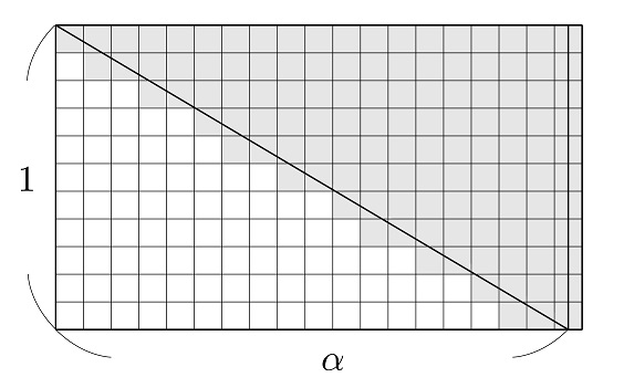
Figure 9. Realization of non-integer $\alpha$

Let us return to the quadratic Wishart case for general $P_{n}$ with parameter $\underline{k}$ as in (2.2) such that $m_{1},m_{2}\in\mathbb{Z}_{\geq 0}$ are fixed. Note that $m_{2}(n)$ in the previous discussion is now $m_{2}(n)=m_{2}b_{n}$. Set $N_{n}:=m_{1}n+m_{2}b_{n}$. We have

$$E_{\underline{k}}=\left\{\xi=\begin{pmatrix}\eta\\ \zeta\end{pmatrix}\in\mathrm{Mat}(n\times N_{n},\,\mathbb{R});\;\begin{array}[]{l}\eta=(\eta_{ij})\in\mathrm{Mat}(a_{n}\times N_{n},\,\mathbb{R}),\\ \zeta=(\zeta_{ij})\in\mathrm{Mat}(b_{n}\times N_{n},\,\mathbb{R})\\ \eta_{ij}=0\text{ if }j\leq(m_{1}-1)i,\\ \zeta_{ij}=0\text{ if }M(i,j)\not\in\{1,2,\dots,m_{1}+m_{2}\}\end{array}\right\},$$

where $M(i,j):=j-m_{1}a_{n}-(m_{1}+m_{2})(i-1)$.

Corollary 4.14.

Let $\{P_{n}\}_{n}$ be a sequence of generalized dual Vinberg cones such that $\lim_{n\to\infty}a_{n}/n=c\in(0,1]$. Let $\underline{k}$ be a vector as in (2.2) such that $m_{1},m_{2}$ are fixed. Set $\kappa:=1/(1-m_{1})$ and $\gamma:=1-\bigl{(}m_{1}+m_{2}(1-c)\bigr{)}/c$. Then, the Stieltjes transform ${T}(z)$ of the limiting eigenvalue distribution of $Q_{\underline{k}}(\xi_{n})/n$ with i.i.d. matrices $\xi_{n}\in E_{\underline{k}}$ is given for $z\in\mathbb{C}^{+}$ as

$${T}(z)=-\frac{1}{v}-\frac{c}{zW_{\kappa,\gamma}(-\frac{cv}{z})}-\frac{c\gamma+1-c}{z}=\frac{\exp_{\kappa}\bigl{(}W_{\kappa,\gamma}(-vc/z)\bigr{)}-1}{v}-\frac{1-c}{z}.$$

The properties of absolute continuity and support of the limiting measure can be derived analogously to those obtained in Theorem 4.8 for $c=1$.

Proof.

We construct a variance profile $\sigma$ from $E_{\underline{k}}$ likely to (4.22). We embed the rectangular matrix $\xi_{n}\in E_{\underline{k}}$ in a square matrix $Y(\xi_{n})=\begin{pmatrix}0&\xi_{n}\\ {}^{t}\xi_{n}&0\end{pmatrix}$, and set $V_{n}=\left\{Y(\xi_{n});\;\xi_{n}\in E_{\underline{k}}\right\}$. Set $\displaystyle p^{\prime}=\lim_{n\to\infty}\frac{n}{n+N_{n}}=\frac{1}{1+m_{1}+m_{2}(1-c)}$. Let $\sigma$ be a function $[0,1]\times[0,1]\to\mathbb{R}_{\geq 0}$ defined by

$$\sigma(x,y)=\begin{cases}v&(\text{$x<cp^{\prime}$ and $y\geq p^{\prime}+m_{1}x$})\\ v&(\text{$x\geq p^{\prime}$ and $0\leq y\leq\min\{(x-p^{\prime})/m_{1},cp^{\prime}\}$}),\\ 0&(\text{otherwise}).\end{cases}$$

Then, we can show that $\sigma$ is the variance profile of $V_{n}$. On the other hand, let us consider a subspace $E^{\prime}_{\underline{k}}:=\left\{\xi=\begin{pmatrix}\eta\\ \zeta\end{pmatrix}\in E_{\underline{k}};\;\zeta=0\right\}$ of $E_{\underline{k}}$, and let $V^{\prime}_{n}=\left\{Y(\xi_{n});\;\xi_{n}\in E^{\prime}_{\underline{k}}\right\}$. Then, $\sigma$ is also the variance profile of $V^{\prime}_{n}$. Thus, we consider equivalently the limiting eigenvalue distribution of $V^{\prime}_{n}$, and that of covariance matrices on $E^{\prime}_{\underline{k}}$. If $\xi_{n}=\begin{pmatrix}\eta_{n}\\ 0\end{pmatrix}\in E^{\prime}_{\underline{k}}$, then $Q_{\underline{k}}(\xi_{n})=\begin{pmatrix}\eta_{n}{}^{\,t\!}\eta_{n}&0\\ 0&0\end{pmatrix}$, and thus it is enough to study the limiting eigenvalue distribution of $\eta_{n}{}^{\,t\!}\eta_{n}$. The variance profile of $\eta_{n}{}^{\,t\!}\eta_{n}$ has a trapezoidal form (4.22) (illustrated by (4.23)) with parameters $\alpha=m_{1}$ and $p=\lim_{n}\frac{a_{n}}{a_{n}+N_{n}}=\frac{c}{c+m_{1}+m_{2}(1-c)}$. Applying Proposition 4.7, we see that the corresponding Stieltjes transform $T_{1}(z)$ is given by

$$T_{1}(z)=T_{\kappa,\gamma}(z)\quad\text{with}\quad\kappa=\frac{1}{1-m_{1}},\quad\gamma=\frac{2p-1}{p}=\frac{c-m_{1}-m_{2}(1-c)}{c}.$$

In general, for two symmetric matrices $A_{i}$ $(i=1,2)$ of size $n_{i}$, the Stieltjes transform $S(z)$ of $\mathrm{diag}(A_{1},\,A_{2})/(n_{1}+n_{2})$ can be described by using the Stieltjes transforms $S_{i}(z)$ of $A_{i}/n_{i}$ $(i=1,2)$ as

$$S(z)=S_{1}\left(\frac{n_{1}+n_{2}}{n_{1}}z\right)+S_{2}\left(\frac{n_{1}+n_{2}}{n_{2}}z\right)\quad(z\in\mathbb{C}^{+}).$$

In our situation, we have $(n_{1},n_{2})=(a_{n},b_{n})$ and $(A_{1},A_{2})=(\eta_{n}{}^{\,t\!}\eta_{n},0)$. Hence, we have $S_{2}(z)=-\frac{1}{z}$ and $S_{1}(z)$ is the Stieltjes transform of $\eta_{n}{}^{\,t\!}\eta_{n}/{a_{n}}$ so that $\lim_{n\to\infty}S_{1}(z)=T_{1}(z)$. Thus, taking the limit $n\to\infty$, we see that the limiting Stieltjes transform $T(z)$ corresponding to $E^{\prime}_{\underline{k}}$, and hence to $E_{\underline{k}}$ is given as

$$\begin{array}[]{r@{\ }c@{\ }l}T(z)&=&\displaystyle T_{1}\left(\frac{z}{c}\right)+S_{2}\left(\frac{z}{1-c}\right)=T_{\kappa,\gamma}\left(\frac{z}{c}\right)-\frac{1-c}{z}\\[8.00003pt] &=&\displaystyle-\frac{1}{v}-\frac{c}{zW_{\kappa,\gamma}(-vc/z)}-\frac{c\gamma+1-c}{z},\end{array}$$

whence we obtain the corollary. ∎∎

Remark 4.15.

In the Figures 12-12 we present simulations of $\underline{k}$-indexed Wish-art ensembles $X_{n}=Q_{\underline{k}}(\xi_{n})$ on the symmetric cone $\mathrm{Sym}(n,\mathbb{R})^{+}$ (i.e. $c=1$), for $n=4000$ and $N=|\underline{k}|=2n$ with parameters $\alpha=m_{1}=1/2$, $1$ and $2$, respectively. We have $\gamma=-1$ and $\kappa=2,\infty,-1$ respectively. The red line is the graph of $d(x)$ generated by the R program from its Stieltjes transform given in Corollary  4.11. In two first cases, the limiting density $d(x)$ is continuous on $\mathbb{R}$ with compact support contained in $(0,\infty)$. The last case $(\kappa,\gamma)=(-1,-1)$ corresponds to $(\kappa^{\prime},\gamma^{\prime})=(1,0)$ which is the classical Wishart case with $C=1$. Thus its density explodes to $\infty$ at 0.

Figure 10. Simulation for $\alpha=1/2$

Figure 11. Simulation for $\alpha=1$

Figure 12. Simulation for $\alpha=2$

Remark 4.16.

Let $Y_{n}$ be a rectangular $n\times p$ i.i.d. matrix with variance profile $\sigma(x,y)$, and assume that $\lim_{n\to\infty}p/n=c$. In papers Hachem at al. [2005, 2006], Hachem et al. [2008] a functional equation $\tau(u,z)=\bigl{(}-z+\int_{0}^{1}\sigma(u,v)\bigl{(}1+c\int_{0}^{1}\sigma(x,v)\tau(x,z)dx\bigr{)}^{-1}dv\bigr{)}^{-1}$ is given to get the limiting Stieltjes transform $f(z)$ for the rescaled random matrices $Y_{n}Y_{n}^{*}$, as the integral $\int_{0}^{1}\tau(u,z)du$. This equation appears in Girko [1990] in the setting of Gram matrices based on Gaussian fields (cf. Hachem at al. [2006, Remark 3.1]).

However, thanks to symmetry, solving the equations  (4.24) resulting from Theorem 2.3 is easier than solving the last functional-integral equation for $\tau(u,z)$. Therefore we opted for variance profile method for Gaussian and Wigner ensembles as the main tool of studying Wishart ensembles of Vinberg matrices.

5. Wigner and Wishart Ensembles related to Generalized Vinberg cones

In this section, we consider the dual cone $Q_{G_{n}}$ of $P_{n}$, which is realized as a minimal matrix form in the sense of Yamasaki and Nomura [2015] as follows. Let $\mathcal{V}_{n}$ be a subspace of $\mathrm{Sym}(a_{n}(b_{n}+1),\,\mathbb{R})$ defined by

$$\mathcal{V}_{n}:=\left\{\mathrm{diag}\left(\begin{pmatrix}x&y_{1}\\ {}^{t\!}y_{1}&d_{1}\end{pmatrix},\dots,\begin{pmatrix}x&y_{b_{n}}\\ {}^{t\!}y_{b_{n}}&d_{b_{n}}\end{pmatrix}\right);\;\begin{array}[]{l}x\in\mathrm{Sym}(a_{n},\mathbb{R}),\\ y_{1},\dots,y_{b_{n}}\in\mathbb{R}^{a_{n}},\\ d_{1},\dots,d_{b_{n}}\in\mathbb{R}\end{array}\right\}.$$ (5.34)

Then, the dual cone $Q_{G_{n}}$ is described as $Q_{G_{n}}:=\mathcal{V}_{n}\cap\mathrm{Sym}(a_{n}(b_{n}+1),\,\mathbb{R})^{+}$.

We consider Wigner Ensembles $V_{n}\in\mathcal{V}_{n}$ and quadratic Wishart Ensembles $X_{n}\in Q_{G_{n}}$ as those in the sense of $\mathrm{Sym}(a_{n}(b_{n}+1),\,\mathbb{R})$. Assume that $\lim_{n\to+\infty}a_{n}=\infty$. By the theory of lower rank perturbation (see Tao [2012, §2.4.1], for example), the study of eigenvalue distributions of these ensembles boils down to the study of the eigenvalue distributions of $x$ and, after suitable normalization, the limiting eigenvalue distributions of $V_{n}$ and $X_{n}$ are the same as for $x\in\mathrm{Sym}(a_{n},\,\mathbb{R})$.

This essential difference in the Random Matrix Theory for the cones $Q_{G_{n}}$ and $P_{n}$ may be explained by a substantial difference between the cones $Q_{G_{n}}$ and $P_{n}$ in terms of numbers of sources in the sense of Yamasaki and Nomura [2015]. In the case $P_{n}$, there is only one source so that $P_{n}$ can be realized in a usual matrix form. On the other hand, $Q_{G_{n}}$ has $b_{n}$ sources so that $b_{n}$ copies of a usual matrix form appear.

6. Acknowledgements

The authors would like to express their sincere gratitude to Professor H. Ishi for strong encouragement and invaluable comments on this work. The authors are very grateful to Professor J. Najim for significant methodological and bibliographical indications for this work and to Professor C. Bordenave for discussions on Theorem 2.3. The authors thank the Scientific Committee of the CIRM Luminy 2020 Conference ”Mathematical Methods of Modern Statistics” (MMMS 2) for giving the possibility to present this work. We thank numerous participants of MMMS 2 for their comments and remarks.

This research was carried out while the first author spent the winter semester of 2018 at Laboratoire de Mathématiques LAREMA under the support of Grant-in-Aid for JSPS fellows (2018J00379).

References

- Ahlfors [1979] Ahlfors, L. (1979), Complex Analysis, An introduction to the theory of analytic functions of one complex variable. Third edition. International Series in Pure and Applied Mathematics. McGraw-Hill Book Co., New York, 1978.
- Amari and Ohara [2011] Amari, S., Ohara, A. (2011), Geometry of -exponential family of probability distributions, Entropy 13, no. 6, 1170–1185.
- Anderson et.al. [2010] Anderson, G. W., Guionnet, A., Zeitouni, O. (2010), An Introduction to Random Matrices, Cambridge University Press.
- Anderson and Zeitouni [2006] Anderson, G. W., Zeitouni, O. (2006), A CLT for a band matrix model, Probab. Theory Relat. Fields 134, 283–338.
- Andersson and Wojnar [2004] Andersson, S. A., Wojnar, G. G. (2004), Wishart distributions on homogeneous cones, J. Theoret.Probab. vol 17, 781–818.
- Bai et al. [2018] Bai, Z., Choi, K., Fujikoshi, Y. (2018), Consistency of AIC and BIC in estimating the number of significant components in high-dimensional principal component analysis, Ann. Statist., 46(3), 1050–1076.
- Bai and Silverstein [2010] Bai, Z., Silverstein, J. W. (2010), Spectral Analysis of Large Dimensional Random Matrices, Springer Series in Statistics, Springer, New York, Second Edition.
- Benaych-Georges [2009] Benaych-Georges, F. (2009), Rectangular random matrices, related convolution, Probab. Theory Related Fields, 144, no. 3, 471–515.
- Bordenave [2019] Bordenave, C. (2019), Lecture notes on random matrix theory, https://www.math.univ-toulouse.fr/ bordenave/IMPA-RMT.pdf.
- Borodin [1999] Borodin, A. (1999), Biorthogonal ensembles, Nuclear Phys. B536, no. 3, 704–732.
- Brillinger [1966] Brillinger, D. R. (1966), The analyticity of the roots of a polynomial as functions of the coefficients, Math. Mag. 39 (1966), 145–147.
- Bun et al. [2017] Bun, J., Bouchaud, J. P., Potters, M. (2017), Cleaning large correlation matrices: Tools from Random Matrix Theory, Physics Reports 666, 1–109.
- Candès and Tao [2005] Candès, E., Tao, T. (2005), Decoding by linear programming, IEEE Transactions on Information Theory 51(12), 4203–4215.
- Chafaï [2009] Chafaï, D. (2009), SINGULAR VALUES OF RANDOM MATRICES, Lecture Notes, http://djalil.chafai.net/docs/sing.pdf
- Cheliotis [2018] Cheliotis, D. (2018), Triangular random matrices and biorthogonal ensembles, Statist. Probab. Letter 134, 36–44.
- Claeys and Romano [2014] Claeys, T., Romano, S. (2014), Biorthogonal ensembles with two-particle interactions, Nonlinearity 27, no. 10, 2419–2443.
- Corless et al. [1996] Corless, R. M., Gonnet, G. H., Hare, D. E. G., Jeffrey, D. J., Knuth, D. E. (1996), On the Lambert function, Adv. Comput. Math. 5, no. 4, 329–-359.
- Diaconis [2003] Diaconis, P. (2003), Patterns in eigenvalues: the 70th Josiah Willard Gibbs lecture, Bull. Amer. Math. Soc. 40, 155–178.