Theoretical analysis for flattening of a rising bubble in a Hele-Shaw cell

Abstract

We calculate the shape and the velocity of a bubble rising in an infinitely large and closed Hele-Shaw cell using Park and Homsy’s boundary condition which accounts for the change of the three dimensional structure in the perimeter zone. We first formulate the problem in the form of a variational problem, and discuss the shape change assuming that the bubble takes elliptic shape. We calculate the shape and the velocity of the bubble as a function of the bubble size, gap distance and the inclination angle of the cell. We show that the bubble is flattened as it rises. This result is in agreement with experiments for large Hele-Shaw cells.

I Introduction

Motion of a bubble moving in a Hele-Shaw cell under gravity is a classical problem first discussed by Taylor and Saffman in 1959Taylor and Saffman (1959), yet there remains an unsolved problem. To make the discussion clear, we restrict ourselves to the problem of an isolated bubble rising under gravity in a closed and infinitely large Hele-Shaw cell. The problem is how the shape of the rising bubble is determined.

Taylor and SaffmanTaylor and Saffman (1959) showed that the set of equations determining the shape and the velocity of the bubble in steady state can be solved analytically if the effect of surface tension is ignored. They also showed that there are infinite number of such solutions, and further condition is needed to determine the shape uniquely. They made a conjecture which determines the unique solution observed in experiments, but they could not justify the physical or mathematical origin of the conjecture.

Twenty seven years later, TanveerTanveer (1986) showed that the degeneracy of the Taylor-Saffman solution is removed if the surface tension is accounted for, but there still remain multiple branches of exact solutionsTanveer (1987). Furthermore, many other solutions have been found in recent yearsCrowdy (2009); Green and Vasconcelos (2014); Green et al. (2017).

Experimentally, the multiplicity of the solutions is puzzling. It has been observed that if the rising velocity $U$ is small, the bubble takes a circular shape, and with increasing the velocity, the bubble deforms to ellipse, and cambered ellipseEck and Siekmann (1978). Kopf-Sill and HomsyKopf-Sill and Homsy (1988) studied the bubble shape when various parameters, such as rising speed, bubble size, liquid viscosity are varied. They have shown that for a bubble rising in a large cell, the bubble shape changes from circle to flattened ellipse (with long axis perpendicular to the moving direction), but no theory has been given to explain such shape change.

Recently, the rising bubble has been studied both theoretically and experimentally and also by simulation Eri and Okumura (2011); Yahashi et al. (2016); Okumura (2018); Keiser et al. (2018); Shukla et al. (2019); Wang et al. (2016); Tihon and Ezeji (2019). Theories have been given for the rising velocity of a bubble of given shapeEck and Siekmann (1978); Meiburg (1989), but no theories have been given to predict the shape of the bubble as far as we know.

The lack of the theory predicting the bubble shape is related to the fact, first shown by TanveerTanveer (1986), that perturbative calculation cannot be performed for the shape change of the bubble. One expects that when a bubble starts to move, it changes the shape from circular to elliptic. Tanveer, however, has shown that the circular solution is an isolated solution which is always valid, and other solutions cannot be obtained by perturbation method.

There is other difficulty in calculating the bubble shape. The bubble shape we are talking about is the shape of the perimeter in the 2D plane parallel to the cell wall. However, the perimeter of the bubble in the Hele-Shaw cell is not a line, but a region having a length of the order of the gap thickness. The 3D structure of this region influences the 2D shape of the bubbleKopf-Sill and Homsy (1988); Meiburg (1989). In the classical works of Tayler-Saffman and Tanveer, the interfacial region was regarded as a line across which the pressure changes discontinuously. The discontinuity in the pressure is given by the air/fluid surface tension times twice of the mean curvature of the interface, i.e., the average of the curvature in the plane perpendicular to the cell wall, and that in the plane parallel to the cell wall. Taylor and Saffman conducted the analysis assuming that the first curvature is dominant and is constantTaylor and Saffman (1959). This assumption becomes equivalent to setting the surface tension zero in the present problem. Tanveer took into account of the effect of the second curvature, but this was not enough since the first curvature also changes when the interface is moving as it was first shown by Bretherton(Bretherton, 1961). Taylor and Saffman discussed this effect in their classical workSaffman and Taylor (1958); Taylor and Saffman (1959), but did not develop a theory for it. Park and Homsy considered this effect and derived a new boundary condition for the perimeterPark and Homsy (1984). Their boundary condition makes the problem non-linear and thus difficult to handle analytically. Accordingly, their boundary condition has not been used in previous studies apart from in numerical simulationsMeiburg (1989).

In this paper, we shall calculate the deformation of a rising bubble using Park-Homsy’s boundary condition. We take an approach different from previous ones. We first show that the set of equations to be solved can be derived by a minimization of certain functional for the shape change of the bubble, and then determine the shape assuming a elliptical shape of the bubble. This approach is not exact, but it allows us to have an analytical expression for the shape and the velocity of the bubble as a function of various experimental parameters. The same approach has been used in many other problems Xu et al. (2016); Man and Doi (2016); Di et al. (2018); Guo et al. (2019).

The structure of this paper is as follows. In Section II, we review the boundary condition by Park and Homsy and state the problem in the form of a variational problem. In Section III, we consider the motion of a bubble in a Hele-Shaw cell and derive a reduced model using the variational principle. In Section IV, we analyze the reduced model and discuss the shape and the velocity of the bubble as a function of various physical parameters. Finally we conclude briefly in Section V.

II Variational formulation

II.1 Basic equation

We consider a very large Hele-Shaw cell filled with a liquid of viscosity $\mu$ tilted against the horizontal plane with angle $\alpha$ (see Fig, 1). Inside the liquid there is a small air bubble which rises with certain velocity $U$ due to gravity. The gap distance $d_{0}$ of the Hele-Shaw cell is assumed to be much smaller than the bubble size, and the capillary length $\sqrt{\gamma/\rho g}$ (where $\rho$ and $\gamma$ are the density and the surface tension of the liquid respectively). Therefore the bubble takes a pancake shape of thickness $d_{0}$ between the cell wall; the thickness of the liquid film between the bubble and the plates is ignored.

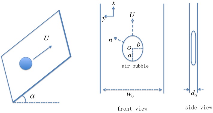
Figure 1: A bubble in a Hele-Shaw cell.

We take $x$-$y$ coordinate in the plane of the Hele-Shaw cell, with the y axis being in the horizontal plane. Let $\bm{u}(\bm{r})$ be the depth-average 2D velocity of the fluid at point $\bm{r}$, $\bm{u}$ satisfies the Darcy equation,

$$\bm{u}=-k(\nabla p+\rho g\sin\alpha\mathbf{e}_{x}),$$ (1)

where $k=\frac{d_{0}^{2}}{12\mu}$, $p$ is the pressure and $\mathbf{e}_{x}$ is the unit vector along the $x$ axis. The velocity $\bm{u}$ satisfies the incompressible condition,

$$\nabla\cdot\bm{u}=0.$$ (2)

Equations (1) and (2) gives the Laplace equation for $p$

$$\nabla^{2}p=0.$$ (3)

Therefore $\bm{u}$ is obtained if the boundary condition for $p$ is known.

Park and Homsy Park and Homsy (1984) conducted asymptotic analysis for the problem and derived the following effective boundary condition for the pressure $p$(see also Reinelt (1987)),

$$p =-\frac{2\gamma}{d_{0}}(1+\beta Ca_{n}^{2/3}+\cdots)-\frac{\gamma}{R(s)}(\frac{\pi}{4}+O(Ca_{n}^{2/3})),$$ (4)

$$[u] =O(Ca_{n}^{2/3}).$$ (5)

Here $Ca_{n}=\frac{\mu|\bm{u}\cdot\mathbf{n}|}{\gamma}$ is the capillary number defined for the normal velocity $u_{n}=\bm{u}\cdot\mathbf{n}$ at the boundary of the bubble, $R(s)$ is the local radius of the curvature of the bubble, and $\beta$ is a numerical constant which is equal to $3.8$ when the interface is locally advancing($u_{n}>0$) and equal to $-1.9$ when the interface is receding($u_{n}<0$). $[u]$ is the difference between the velocity $u_{n}$ and the moving velocity of the bubble boundary. Introducing the velocity $U^{*}=\gamma/\mu$, the capillary number $Ca_{n}$ is written as

$$Ca_{n}=\frac{|u_{n}|}{U^{*}}$$ (6)

When $Ca_{n}$ is small, we can consider the leading order only, and Equ.( 4) becomes

$$p =-\frac{2\gamma}{d_{0}}(1+\beta Ca_{n}^{2/3})-\frac{\gamma}{R(s)}\frac{\pi}{4},$$ (7)

$$[u] =0.$$ (8)

Here we have kept the term $\frac{2\gamma}{d_{0}}Ca_{n}^{2/3}$ since $Ca_{n}^{2/3}/d_{0}$ may be comparable with ${1}/{R(s)}$ when $d_{0}/R(s)$ is small. Furthermore, the constant $\frac{2\gamma}{d_{0}}$ in Equ. (7) can be ignored by shifting $p$ by a constant. Therefore we finally have the following boundary conidition

$$p=-\frac{2\gamma}{d_{0}}\beta Ca_{n}^{2/3}-\frac{\gamma}{R(s)}{\frac{\pi}{4}}.$$ (9)

The other boundary condition far from the bubble is obtained from the condition that there is no flow:

$$\mbox{for }|\bm{r}|\to\infty,\qquad p\to-{\rho gx\sin\alpha}.$$ (10)

Equ. (3) and the boundary conditions (9) and (10) compose the basic equations for the rising bubble problem in the Hele-Shaw cell.

II.2 Variational formulation

The basic equations described above can be derived from a variational principle similar to the Onsager variational principle (Doi, 2013). We define a functional called Rayleighian $\mathcal{R}[\bm{u}(\bm{r})]$ which is a functional of the velocity field $\bm{u}(\bm{r})$. $\mathcal{R}[\bm{u}(\bm{r})]$ is chosen in such a way that the minimum condition of the functional gives the same set of equations given in the previous subsection. The Rayleighian $\mathcal{R}[\bm{u}(\bm{r})]$ consists of two parts: one is the energy dissipation part $\Phi[\bm{u}(\bm{r})]$ which is related to the energy dissipation (or entropy production) created in the system when the viscous fluid is flowing with velocity field $\bm{u}(\bm{r})$, and the other part is related to the free energy change rate $\dot{A}[\bm{u}(\bm{r})]$ when the fluid elements are moving with velocity $\bm{u}(\bm{r})$.

$$\mathcal{R}[\bm{u}(\bm{r})]=\Phi[\bm{u}(\bm{r})]+\dot{A}[\bm{u}(\bm{r})].$$ (11)

In the present problem, the functional of the dissipation $\Phi[\bm{u}(\bm{r})]$ is given by the sum of two integrals,

$$\Phi[\bm{u}(\bm{r})]=\Phi_{bulk}[\bm{u}(\bm{r})]+\Phi_{Breth}[\bm{u}(\bm{r})],$$ (12)

where

$$\Phi_{bulk}[\bm{u}(\bm{r})]=\frac{d_{0}}{2k}\int_{\Omega^{c}}\bm{u}^{2}dxdy$$ (13)

stands for the energy dissipation in the bulk, and

$$\Phi_{Breth}[\bm{u}(\bm{r})]=\frac{6\mu(U^{*})^{1/3}}{5}\int_{\partial\Omega}\beta(u_{n})u_{n}^{5/3}ds$$ (14)

stands for the extra energy dissipation due to the motion of the perimeter. In Equ. (13), $\Omega^{c}$ denotes the 2D region in the Hele-Shaw cell occupied by the liquid and $\partial\Omega$ denotes the inner boundary of $\Omega^{c}$. The function $\beta(u_{n})$ takes the value of $\beta_{1}=3.8$ when $u_{n}>0$ and the value $\beta_{2}=-1.9$ when $u_{n}<0$. We shall call $\Phi_{bulk}$ bulk dissipation, and $\Phi_{Breth}$ Bretherton dissipation. Detailed discussion on Equ.(14) is given in Appendix A.

The free energy of the system is given by the sum of the gravitational energy and the surface energy

$$A=\int_{\Omega^{c}}{\rho gd_{0}x\sin\alpha}dxdy+\frac{\pi\gamma d_{0}}{4}\int_{\partial\Omega}ds.$$ (15)

$\dot{A}$ is given by the time derivative of $A$, and is calculated as

$$\dot{A}={\rho gd_{0}\sin\alpha}\int_{\Omega^{c}}\bm{u}\cdot\bm{e_{x}}dxdy+\frac{\pi\gamma d_{0}}{4}\int_{\partial\Omega}u_{n}\kappa ds,$$ (16)

where $\kappa=\frac{1}{R(s)}$ is the local curvature of the boundary $\partial\Omega$.

We minimize the Rayleighian with respect to $\bm{u}$ under the constraint $\nabla\cdot\bm{u}=0$. Introduce a Lagrangian multiplier $d_{0}p$ and denote

$$\mathcal{R}_{p}=\mathcal{R}-d_{0}\int_{\Omega^{c}}p\nabla\cdot udxdy.$$ (17)

By integration by part (noticing that $\mathbf{n}$ points into $\Omega^{c}$),

$$\mathcal{R}_{p}=\mathcal{R}+d_{0}\int_{\partial\Omega}pu_{n}ds+d_{0}\int_{\Omega^{c}}u\cdot\nabla pdxdy.$$

One can easily verify that the Euler-Lagrange equation of the functional $\mathcal{R}_{p}$ gives the equation (1) and the boundary condition (9) in the previous subsection.

The above variational formula is similar to that of the standard Onsager principleXu et al. (2016); Man and Doi (2016); Di et al. (2018); Guo et al. (2019). The only difference is that the dissipation function is not a quadratic form with respect to $\bm{u}$. This is due to the non-quadratic term on the boundary $\partial\Omega$ arising from the Bretherton energy dissipation. In the following, we will use the variational formula as an approximation tool to study the shape changes of the rising bubble in the Hele-Shaw cell.

III Derivations of a reduced model for a rising bubble

III.1 Ansatz of the problem

To analyse the shape changes of the bubble, we assume that the bubble is elliptic as shown in Fig. 1. It has been shown both theoretically Taylor and Saffman (1959) and experimentallyKopf-Sill and Homsy (1988) that the elliptic shape is a good approximation when the deviation from the circular shape is small The radii of the ellipse in $x$ and $y$ directions are $a$ and $b$ respectively. The vertical velocity of the center of the bubble is $U$. Since the volume $V_{0}$ of the bubble is estimated to be $\pi abd_{0}$ (where the volume of the liqid between the gas and the wall and that in the perimeter region is ignored), and is constant, $b$ is given by

$$b=\frac{V_{0}}{\pi d_{0}a}.$$

So there are two parameters to be determined, $a$ and $U$. In the following we will use the variational principle to derive a reduced dynamic model for them.

III.2 Free energy

The free energy of the system consists of the interface energy and the gravitational energy. The interface energy is given by

$$A_{surf}=2\pi\gamma ab+\frac{\pi\gamma d_{0}L}{2},$$ (18)

where $L$ is the 2D contour length of the boundary of the ellipse. Since $\pi ab=V_{0}/d_{0}$ is constant, the time derivative of $A_{surf}$ is calculated as

$$\dot{A}_{surf}=\frac{\pi\gamma d_{0}}{2}\dot{L}.$$ (19)

Using the approximation $L\approx\pi(\frac{3}{2}(a+b)-\sqrt{ab})$, we have

$$\dot{A}_{surf}=\frac{3\pi^{2}\gamma d_{0}}{4}(1-\frac{b}{a})\dot{a}.$$ (20)

The gravitational energy is given by $A_{grav}=-\rho gX\sin\alpha V_{0}$, where $X$ is the $x$ coordinate of the center of mass of the bubble. Since $\dot{X}=U$, the time derivative of the gravitational energy is written as

$$\dot{A}_{grav}=-\rho gV_{0}U\sin\alpha.$$ (21)

Therefore $\dot{A}=\dot{A}_{grav}+\dot{A}_{surf}$ is given by

$$\dot{A}=-\rho gV_{0}U\sin\alpha+\frac{3\pi^{2}\gamma d_{0}}{4}(1-\frac{b}{a})\dot{a}.$$ (22)

III.3 Energy dissipation functions.

The energy dissipation can also be expressed in terms of $\dot{a}$ and $U$. If $\dot{a}$ and $U$ are given, the velocity field $\bm{u}(\bm{r})$ is calculated, and therefore the functional $\Phi[\bm{u}(\bm{r})]$ can be written as a function $\Phi(\dot{a},U)$. The function $\Phi(\dot{a},U)$ is equal to the minimum value of the functional $\Phi[\bm{u}(\bm{r})]$ for given boundary condition at $\partial\Omega$.

Bulk dissipation. If the origin of the coordinate system is taken at the center of the bubble, the boundary of the bubble is written as

$$x=a\cos\theta,\quad y=b\sin\theta,\qquad\theta\in(0,2\pi].$$

The corresponding outer normal direction is given by

$$\bm{n}=\frac{1}{\sqrt{b^{2}\cos^{2}\theta+a^{2}\sin^{2}\theta}}(b\cos\theta,a\sin\theta)^{T}.$$

When the center is moving at velocity $U$ and $a$ is changing at rate $\dot{a}$, the normal velocity of the boundary $u_{n}=\bm{u}\cdot\bm{n}$ is calculated as

$$u_{n}=Uf_{1}(a/b,\theta)+\dot{a}f_{2}(a/b,\theta),$$

where

$$f_{1}(a/b,\theta) = \frac{\cos\theta}{\sqrt{\cos^{2}\theta+(a/b)^{2}\sin^{2}\theta}}$$ (23)

$$f_{2}(a/b,\theta) = \frac{\cos 2\theta}{\sqrt{\cos^{2}\theta+(a/b)^{2}\sin^{2}\theta}}$$ (24)

If the velocity $u_{n}$ at the boundary is given, the velocity field $\bm{u}(\bm{r})$ in the bulk is given by $\bm{u}=-(1/k)\nabla\tilde{p}$, where $\tilde{p}$ is the solution of the Laplace equation (3) satisfying the boundary condition $\bm{n}\nabla\tilde{p}=-ku_{n}$ at $\partial\Omega^{c}$, and $\nabla\tilde{p}\to 0$ at infinitely far from the bubble. The solution of this equation is written as

$$\tilde{p}(x,y)=\frac{r_{0}U}{k}\psi_{1}(\frac{x}{r_{0}},\frac{y}{r_{0}})+\frac{r_{0}\dot{a}}{k}\psi_{2}(\frac{x}{r_{0}},\frac{y}{r_{0}}),$$ (25)

where $\psi_{i}$ ($i=1,2$) is the solution of the following dimensionless equation

$$\left\{\begin{array}[]{ll}-\Delta\psi_{i}=0,&\hbox{in }\hat{\Omega}^{c}\\ \nabla\psi_{i}\cdot\tilde{\mathbf{n}}=f_{i}(a/b,\theta),&\hbox{on }\partial\hat{\Omega}\\ \nabla\psi_{i}\cdot\tilde{\mathbf{n}}\rightarrow 0&\hbox{as }|\hat{\mathbf{r}}|\rightarrow\infty.\end{array}\right.$$ (26)

Here the radius $r_{0}=\sqrt{ab}$ is taken to be the unit of length, and the domain $\hat{\Omega}^{c}$ is defined by $\hat{\Omega}^{c}:=\{({x}/{r_{0}},{y}/r_{0})|(x,y)\in{\Omega}^{c}\}$.

Therefore the energy dissipation function in the bulk region is computed as

$$\Phi_{bulk} =\frac{6\mu}{d_{0}}\int_{\Omega^{c}}(k\nabla\tilde{p})^{2}dxdy=\frac{6\mu}{d_{0}}\int_{\hat{\Omega}^{c}}|{r_{0}U}\nabla\psi_{1}+{r_{0}\dot{a}}\nabla\psi_{2}|^{2}d\hat{x}d\hat{y}$$

$$=\frac{6\mu r_{0}^{2}}{d_{0}}(k_{11}U^{2}+2k_{12}U\dot{a}+k_{22}\dot{a}^{2}),$$ (27)

where

$$k_{ij}=\int_{\hat{\Omega}^{c}}\nabla\psi_{i}\cdot\nabla\psi_{j}d\hat{x}d\hat{y}$$ (28)

By integration by part, the coefficients $k_{ij}$ can be written as

$$k_{ij}=\int_{\partial\hat{\Omega}}\psi_{i}f_{j}(a/b,\hat{\theta})d\hat{s},$$ (29)

For elliptic bubble, the Laplace equation(26) can be solved analytically and $k_{ij}$ is calculated analytically(see Appendix B)

$$k_{11}=\frac{\pi b}{a},\qquad k_{12}=0,\qquad k_{22}=\frac{\pi b}{2a}$$ (30)

It is important to note $k_{12}$ is zero. This implies that there is no term which couples the translational motion and the shape change in the bulk dissipation $\Phi_{bulk}$. In other words, the bubble remains circular if the Bretherton dissipation $\Phi_{Breth}$ is not considered. The fact that $k_{12}$ becomes zero for ellipse can be shown by symmetry argument. Since the elliptic bubble is symmetric with respect to $y$ axis, the dissipation function must be even with respect to $U$, i.e. $\Phi_{bulk}(\dot{a},U)=\Phi_{bulk}(\dot{a},-U)$. This gives $k_{12}=0$.

Bretherton dissipation. Given $u_{n}$, the Bretherton dissipation can be calculated straightforwardly by Equ. (14):

$$\Phi_{Breth} =\frac{6\mu}{5}\int_{\partial\Omega}\beta(u_{n})u_{n}^{2}(\frac{\mu|u_{n}|}{\gamma})^{-\frac{1}{3}}ds$$

$$=\frac{6\mu^{2/3}\gamma^{1/3}r_{0}}{5}\int_{0}^{2\pi}\beta(\theta)|f_{1}U+f_{2}\dot{a}|^{5/3}\sqrt{(b/r_{0})^{2}\cos^{2}\theta+(a/r_{0})^{2}\sin^{2}\theta}d\theta.$$ (31)

III.4 Evolution equation

Given $\Phi=\Phi_{bulk}+\Phi_{Breth}$ and $\dot{A}=\dot{A}_{grav}+\dot{A}_{surf}$ as a function of $\dot{a}$ and $U$, the time evolution of the bubble is given by

$$\frac{\partial\Phi}{\partial U}+\frac{\partial\dot{A}}{\partial U}=0,\qquad\frac{\partial\Phi}{\partial\dot{a}}+\frac{\partial\dot{A}}{\partial\dot{a}}=0.$$ (32)

This gives the following equation for $U$ and $\dot{a}$:

$$\frac{{\color[rgb]{0,0,0}12}\mu r_{0}^{2}}{d_{0}}k_{11}U +{2\mu^{2/3}\gamma^{1/3}b}\int_{0}^{2\pi}\beta(\theta)\frac{(f_{1}U+f_{2}\dot{a})f_{1}}{|f_{1}U+f_{2}\dot{a}|^{1/3}}\sqrt{\cos^{2}\theta+(a/b)^{2}\sin^{2}\theta}d\theta$$

$$=\rho gV_{0}\sin\alpha,$$ (33)

$$\frac{{\color[rgb]{0,0,0}12}\mu r_{0}^{2}}{d_{0}}k_{22}\dot{a} +{2\mu^{2/3}\gamma^{1/3}b}\int_{0}^{2\pi}\beta(\theta)\frac{(f_{1}U+f_{2}\dot{a})f_{2}}{|f_{1}U+f_{2}\dot{a}|^{1/3}}\sqrt{\cos^{2}\theta+(a/b)^{2}\sin^{2}\theta}d\theta$$

$$=-\frac{3\pi^{2}\gamma d_{0}}{4}(1-\frac{b}{a}).$$ (34)

This equation can be solved for $\dot{a}$ and $U$, and it determines the time evolution of the bubble shape.

If we are interested only in the steady state of the bubble, we have $\dot{a}=0$. Then the equations (33)-(34) are simplified to

$$\frac{{\color[rgb]{0,0,0}12}\mu r_{0}^{2}}{d_{0}}k_{11}U+{2\mu^{2/3}\gamma^{1/3}r_{0}U^{2/3}}\tilde{k}_{11}=\rho gV_{0}\sin\alpha,$$ (35)

$${2\mu^{2/3}\gamma^{1/3}r_{0}U^{2/3}}\tilde{k}_{12}=-\frac{3\pi^{2}\gamma d_{0}}{4}(1-\frac{b}{a}),$$ (36)

where we have introduced two dimensionless coefficients

$$\tilde{k}_{11} =\int_{0}^{2\pi}\beta(\theta)|f_{1}|^{5/3}\sqrt{(b/r_{0})^{2}\cos^{2}\theta+(a/r_{0})^{2}\sin^{2}\theta}d\theta,$$ (37)

$$\tilde{k}_{12} =\int_{0}^{2\pi}\beta(\theta)\frac{f_{1}f_{2}}{|f_{1}|^{1/3}}\sqrt{(b/r_{0})^{2}\cos^{2}\theta+(a/r_{0})^{2}\sin^{2}\theta}d\theta.$$ (38)

Since $r_{0}=\sqrt{ab}$, $\tilde{k}_{11}$, and $\tilde{k}_{12}$ depends on the ratio $b/a$ only. We call this ratio the shape parameter and denote it by $S$

$$S=\frac{b}{a}.$$ (39)

Fig. 2 shows $\tilde{k}_{11}$, and $\tilde{k}_{12}$ as a function of $S$. When $S$ changes from 0.5 to 2, $\tilde{k}_{11}$ changes significanlty, while $\tilde{k}_{12}$ remains almost constant (changes from 0.85 to 1.1).

Figure 2: Dependence of the coefficients $\tilde{k}_{11}$ and $\tilde{k}_{12}$ on the shape parameter $S=b/a$.

IV Results and discussions

IV.1 Rising velocity

We first discuss the rising velocity of the bubble. The rising velocity is determined by the balance of two forces, the gravity and the frictional force. The gravity is expressed by the dimensionless number $Bo_{\alpha}$ called Bond number

$$Bo_{\alpha}=\frac{\rho gr_{0}^{2}\sin\alpha}{\gamma}.$$ (40)

This represents the effect of inclination angle of the cell. The frictional force is determined by the left hand side of Equ. (35).

The equations (35)-(36) can be rewritten in a dimensionless form as,

$$\frac{12r_{0}^{2}S}{d_{0}^{2}}\frac{U}{U^{*}}+\frac{2r_{0}}{\pi d_{0}}\tilde{k}_{11}\Big{(}\frac{U}{U^{*}}\Big{)}^{2/3}=Bo_{\alpha},$$ (41)

$$\frac{8r_{0}}{3\pi^{2}d_{0}}\tilde{k}_{12}\Big{(}\frac{U}{U^{*}}\Big{)}^{2/3}=1-S,$$ (42)

where $U^{*}={\gamma}/{\mu}$. If we ignore the $\tilde{k}_{11}$ term ( the Bretherton term) in Equ. (41), the velocity is given by

$$U=U^{*}\frac{d_{0}^{2}}{{\color[rgb]{0,0,0}12}r_{0}^{2}S}Bo_{\alpha}=\frac{d_{0}^{2}\rho g\sin\alpha}{{\color[rgb]{0,0,0}12}\mu S}.$$ (43)

This is exactly the velocity for small elliptic bubble given by Taylor and SaffmanTaylor and Saffman (1959). There they did not consider the Bretherton term and $S$ can be chosen freely. If the bubble is circular, the rising velocity becomes

$$U_{circle}=\frac{d_{0}^{2}\rho g\sin\alpha}{{\color[rgb]{0,0,0}12}\mu}.$$ (44)

Fig. 3 shows the velocity plotted against the bond number. The solid lines indicate the velocity calculated by solving the equations (35) and (36), and the dotted and the dashed lines indicate the velocity calculated by Equ.(43) and Equ. (44) respectively. It is seen that the simple circular model gives a reasonable estimate for the rising velocity. The difference between the solid line and the dashed line represents the effect of shape parameter. As we shall show in the following, the rising bubble becomes flattened ($S>1$), and therefore the rising velocity becomes smaller than that of the circular bubble. The difference between the dotted line and the solid line represents the effect of Bretherton dissipation. This term slows down the rising velocity.

The effect of Bretherton dissipation on the rising velocity was considered by Eck and Siekmann Eck and Siekmann (1978). They obtained an expression for the rising velocity of a circular bubble similar to Equ. (41):

$$3+5.28\frac{d_{0}}{2r_{0}}\Big{(}\frac{U^{*}}{U}\Big{)}^{1/3}=\frac{\rho gd_{0}^{2}\sin\alpha}{4\mu U}.$$ (45)

For circular bubble, Equ. (41) gives the following result (with the use of $\tilde{k}_{11}(1)\approx 9.59$)

$$3+3.05\frac{d_{0}}{2r_{0}}\Big{(}\frac{U^{*}}{U}\Big{)}^{1/3}=\frac{\rho gd_{0}^{2}\sin\alpha}{4\mu U}.$$ (46)

The difference between Equ. (45) and Equ. (46) are only in coefficients. They come from the difference in the estimation of the extra energy dissipation at the perimeter: Eck and Siekmann used the analysis of FritzFriz (1965), while we used the Park-Homsy boundary condition. These results are compared in Figure 4 together with the experimental data obtained by Eck and Siekmann Eck and Siekmann (1978). (Notice that in the parameter range shown in Figure 4, our result can be safely represented by the circular bubble since the capillary number $U/U^{*}$ is less than $10^{-3}$ (see Fig. 3 ). ) Both results are qualitatively in agreement with experiments, but Equ. (46) is closer to the experimental data, indicating that the Park-Homsy’s boundary condition (or Bretherton’s analysis) is closer to reality.

Figure 3: The relation between the rising velocity and the gravitational force of a bubble in a Hele-Shaw cell. The solid line is the result of the present theory. The dash-dotted line is the result of Taylor and Saffman theory for circular bubble, Equ. (44). The dotted line is their result for elliptic bubble (Equ. (43)) where the shape parameter $S$ is calculated by Equ. (42)

Figure 4: Comparison between theories and experiment. The dotted line is the result of Eck and Siekman (Equ. (45)) and the solid line is our result (Equ. (46)). The marks are experimental data in Eck and Siekmann (1978)(Fluid 1: $60\%$ isopropanol, $40\%$ water; Fluid 2: $70\%$ glycerine, $18\%$ isopropanol, $12\%$ water).

IV.2 Shape of the rising bubble

Fig. 5 shows how the shape parameter $S=b/a$ changes with the Bond number $Bo_{\alpha}$. The shape parameter $S$ is equal to 1 when $Bo_{\alpha}=0$. As the bubble starts to rise, $S$ becomes larger than $1$ so the bubble is flattened. It is important to note that this shape change is due to Bretherton dissipation. If the Bretherton dissipation is not considered, the circular bubble will rise keeping the circular shape as it was discussed previouslyTaylor and Saffman (1959); Tanveer (1986). The difference of the Bretherton dissipation in the advancing side and the receding side breaks the symmetry of the circular shape and causes the deformation of the bubble.

Fig. 5 shows that the shape change is larger in thick cell than in thin cell. This is because the Bretherton effects become more significant in a thicker Hele-Shaw cell.

Figure 5: The relation between the shape parameter $S=b/a$ and the gravitational force.

Fig. 6 shows the shape parameter plotted against the rising velocity $U/U^{*}$. The dashed line in Fig. 6 represents the following simple equation

$$S=1+0.297\frac{r_{0}}{d_{0}}\cdot\left(\frac{U}{U^{*}}\right)^{2/3},$$ (47)

This equation is obtained from Equ. (36) by putting $\tilde{k}_{12}$ equal to 1.1, the asymptotic value of $\tilde{k}_{12}$ for large $S$ (see Fig. 2). Fig. 6 shows that this simple relation reproduces the numerical results quite well.

Figure 6: The relation between the shape parameter $S=b/a$ and the rising velocity $U/U^{*}$ of the bubble. The dashed line represents Equ. (47).

IV.3 Effect of the bubble size.

We now study how the bubble size affects the rising velocity and its shape changes in a vertical cell($\alpha=\frac{\pi}{2}$). We take the capillary length $l=\sqrt{\gamma/\rho g}$ as a reference length unit. For given thickness of the Hele-Shaw cell, we change the bubble size $r_{0}$, and solved Equ.(35) and (36). The results are shown in Fig. 7 and 8.

Fig. 7 shows the rising velocity $U$ plotted against the bubble size $r_{0}$ for thick ($d_{0}/\ell=0.4$) and thin($d_{0}/\ell=0.2$) cells. It is seen that large bubbles rise with velocity independent of their size. This is because the gravitational force and the frictional force are both proportional to the volume of the bubble in Hele-Shaw cell. The effect can be seen in the simple model (Equ. (44)). Small bubbles rise with size-dependent velocity, which is smaller than the asymptotic value. This is due to the Bretherton dissipation: the Bretherton dissipation is proportional to the length of the perimeter and becomes significant for smaller bubbles.

Careful inspection of Fig. 7 indicates that the rising velocity shows a small maximum as a function of $r_{0}$. The maximum arises from the two competing effects: as the bubble size increases, the effect of Bretherton dissipation decreases, while the effect of bulk dissipation increases due to the flattening of the bubble.

Figure 7: The relation between the rising velocity and the bubble size.

Fig. 8 shows the shape parameter $S=b/a$ plotted against $r_{0}/l$. It is seen that $S$ increases linearly with $r_{0}$ and decreases with the increase of $d_{0}$. Such behaviour can be understood from Equ. (47).

Figure 8: The relation between the shape parameter $S=b/a$ and the bubble size.

V Conclusions

By using a variational principle, we have derived a simple evolution equation for the shape change of a rising bubble in an infinitely large Hele-Shaw cell. The equation explains the flattening of a rising bubble observed in experimentsKopf-Sill and Homsy (1988); Eck and Siekmann (1978). Our analysis shows that the Bretherton dissipations is essential for the flattening. Without this term, the bubble would take a circular shape. We gave quantitative prediction about the shape change and velocity of the bubble. They can be checked experimentally.

In the present analysis, we have ignored the effect of the side boundary of a Hele-Shaw cell. If the size of the Hele-Shaw cell is not large, the boundary effect makes the bubble elongatedTanveer (1986); Tanveer and Saffman (1987); Maxworthy (1986). The competition of the Bretherton effect and the boundary effect should be the reason for the complex shape changes of the bubble in a Hele-Shaw cell. Indeed, Kopf-Sill and Homsy showed that the flattening occurs only for bubbles relatively small compared with the Hele-Shaw cell Kopf-Sill and Homsy (1988). Larger bubbles, on the other hand, are elongatedKopf-Sill and Homsy (1988). More theoretical study is needed to quantify how the two effects together affect the shape change of an air bubble. This will be left for future work.

Appendix

V.1 The Bretherton energy dissipations

In this subsection, we aim to compute the viscous energy dissipation in the vicinity of the boundary of a moving bubble in a Hele-Shaw cell. Since the dissipation is related to the classical analysis in Bretherton’s paper Bretherton (1961), we call it a Bretherton energy dissipation term. We consider a two dimensional problem. It is a long two-dimensional bubble in a channel between two solid boundaries as shown in Fig. 9. The computations below are based on the previous analysis in Bretherton (1961) and Park and Homsy (1984).

Figure 9: A bubble between two plates.

We analyse this problem by a generalized force balance argument. Suppose the fluid pressure in the left side is $P_{2}$ and that in the right side is $P_{1}$. We assume the bubble moves in the right direction. If the bubble moves for a short distance, the liquid in the left part changes with a volume $V_{2}$ and the right part changes with a volume $V_{1}$. Assume the air bubble is incompressible, then we have $V_{1}=V_{2}$. The free energy changes in this process are given by $-(P_{2}V_{2}-P_{1}V_{1})$. If the bubble moves with a velocity $U$, the energy changing rate is given by

$$\dot{A}=-(P_{2}-P_{1})d_{0}U.$$

Here $d_{0}$ is the thickness of the channel. Then the driven force is given by $(P_{2}-P_{1})d_{0}$. If we assume the energy dissipation function, which is half of the energy dissipation rate, is given by

$$\Phi=\frac{1}{s}\xi U^{s}.$$

By the Onsager principle, the driven force is balanced by the fiction force,

$$\xi U^{s-1}=(P_{2}-P_{1})d_{0}.$$ (A1)

By the previous analysis in Park and Homsy (1984), we have the jump condition for pressures

$$P-P_{1}\approx\frac{\gamma}{d_{0}/2}(1+\beta_{1}(C_{a})^{2/3}),\quad P-P_{2}\approx\frac{\gamma}{d_{0}/2}(1-\beta_{2}(C_{a})^{2/3})$$ (A2)

where $P$ is the pressure in the bubble, $C_{a}={\mu U}/{\gamma}$ is the capillary number, $\gamma$ is the surface tension, $\mu$ is the viscosity of the fluid, $d_{0}$ is the distance between the two boundaries of the channel, $\beta_{1}\approx 3.8$ and $\beta_{2}\approx 1.9$ are two positive constants. We then have

$$P_{2}-P_{1}\approx(\beta_{1}+\beta_{2})\frac{2\gamma}{d_{0}}C_{a}^{2/3}=(\beta_{1}+\beta_{2})\frac{2\gamma}{d_{0}}(\frac{\mu U}{\gamma})^{2/3}.$$

Combining it with the equation (A1), we have

$$s=\frac{5}{3},\qquad\xi=2(\beta_{1}+\beta_{2}){\gamma^{1/3}\mu^{2/3}}.$$

This gives a non-quadratic formula for the viscous energy dissipation in the vicinity of the bubble

$$\Phi=\frac{3\xi}{5}U^{5/3}=\frac{6(\beta_{1}+\beta_{2})}{5}\mu(U^{*})^{1/3}U^{5/3}$$ (A3)

where $U^{*}={\gamma}/{\eta}$. The above analysis can also done separately for the head and tail parts. Then we obtain the Bretherton energy dissipation terms

$$\Phi_{head}=\frac{6\beta_{1}}{5}\mu(U^{*})^{1/3}U^{5/3}\approx 4.56\mu(U^{*})^{1/3}U^{5/3},$$ (A4)

$$\Phi_{tail}=\frac{6\beta_{2}}{5}\mu(U^{*})^{1/3}U^{5/3}\approx 2.28\mu(U^{*})^{1/3}U^{5/3},$$ (A5)

where we denote by $\Phi_{head}$ and $\Phi_{tail}$ the dissipation terms in the head and tail parts respectively.

V.2 Solution of the Laplace equation in an infinite domain

When $r_{0}\ll L$, the boundary effect of the Hele-Shaw cell can be ignored. In this case, the Laplace equation in Section 3 can be solved analytically. We suppose $\hat{\Omega}^{c}=\mathbb{R}^{2}\setminus\hat{\Omega}$. Then for $i=1,2$, we need solve

$$\left\{\begin{array}[]{ll}-\Delta\psi_{i}=0,&\qquad\hbox{in }\mathbb{R}^{2}\setminus\hat{\Omega},\\ \tilde{n}\cdot\nabla\psi_{i}=f_{i}(a/b,\hat{\theta}),&\qquad\hbox{on }\partial\hat{\Omega},\\ \psi_{i}\rightarrow const,&\qquad|\mathbf{r}|\hbox{ goes to infinity.}\end{array}\right.$$ (B1)

The equation can be solved by a harmonic mapping method when $\hat{\Omega}$ is elliptic.

Introduce a harmonic mapping in complex plane which maps a circle with radius $R=\hat{a}+\hat{b}$ to the ellipse $\hat{\Omega}$ with radii $\hat{a}=a/r_{0}$ and $\hat{b}=b/r_{0}$,

$$z=\mathcal{F}(\zeta)=\frac{1}{2}(\zeta+\frac{c^{2}}{\zeta}),$$ (B2)

where $\hat{c}^{2}=\hat{a}^{2}-\hat{b}^{2}$. Here we choose the coordinate so that the radius $\hat{a}$ is in the $x$ direction. Its inverse mapping is given by $\zeta=\mathcal{F}^{-1}(z)=z+\sqrt{z^{2}-c^{2}}$. The Laplace equation in an infinite domain outside a circular can by solved explicitly. Actually, if a harmonic function $\phi$ outside a circle satisfies a Neumann boundary condition $\nabla\phi\cdot\mathbf{n}=g$ on the circle $|\zeta|=R$, then it can be computed from its boundary data asHitotumatu (1954):

$$\phi(\zeta)=\frac{1}{\pi}\int_{|\tilde{\zeta}|=R}g(\tilde{\zeta})\ln\frac{1}{|\tilde{\zeta}-\zeta|}d\tilde{\zeta},$$ (B3)

for all $\zeta$ in the infinite domain. Using this formula, we could obtain the solution for $\psi_{i}$ as follows. If we have $\partial_{n}\psi_{i}=f_{i}$ in $\partial_{n}\hat{\Omega}$, after the mapping, we have a harmonic function $\phi_{i}(\zeta)=\psi_{i}(\mathcal{F}\zeta)$ outside a circle. Direct computations give $\partial_{n}\phi_{i}(\zeta)=\frac{\sqrt{\hat{b}^{2}\cos^{2}\tilde{\theta}+\hat{a}^{2}\sin^{2}\tilde{\theta}}}{R}f_{i}(\frac{\hat{a}}{\hat{b}},\tilde{\theta})$, where $\zeta=Re^{i\tilde{\theta}}$. Using Equ. (B3), we obtain

$$\psi_{i}(z)=\phi_{i}(\tilde{r}e^{i\varphi})=\frac{1}{\pi}\int_{0}^{2\pi}f_{i}(\hat{a}/\hat{b},\tilde{\theta})\ln\frac{1}{|Re^{i\tilde{\theta}}-\tilde{r}e^{i\varphi}|}\sqrt{\hat{b}^{2}\cos^{2}\tilde{\theta}+\hat{a}^{2}\sin^{2}\tilde{\theta}}d\tilde{\theta},$$ (B4)

where $(\tilde{r}e^{i\varphi})=\mathcal{F}^{-1}z$.

Then we could compute the coefficients $k_{ij}$ as

$$k_{ij} =\int_{\partial\hat{\Omega}}f_{i}(s)\psi_{j}(s)ds=\int_{0}^{2\pi}f_{i}(\hat{a}/\hat{b},\theta)\phi_{j}({R}e^{i\theta})\sqrt{\hat{b}^{2}\cos^{2}\theta+\hat{a}^{2}\sin^{2}\theta}d\theta$$

$$=\frac{1}{\pi}\int_{0}^{2\pi}f_{i}(\hat{a}/\hat{b},\theta)\int_{0}^{2\pi}f_{j}(\hat{a}/\hat{b},\tilde{\theta})\ln\frac{1}{|Re^{i\tilde{\theta}}-Re^{i\theta}|}$$

$$\qquad\qquad\qquad\qquad\qquad\qquad\qquad\times\sqrt{\hat{b}^{2}\cos^{2}\tilde{\theta}+\hat{a}^{2}\sin^{2}\tilde{\theta}}d\tilde{\theta}\sqrt{\hat{b}^{2}\cos^{2}\theta+\hat{a}^{2}\sin^{2}\theta}d\theta$$

$$=\frac{1}{\pi}\int_{0}^{2\pi}f_{i}(\hat{a}/\hat{b},\theta)\int_{0}^{2\pi}f_{j}(\hat{a}/\hat{b},\tilde{\theta})\ln\frac{1}{\sqrt{(\cos\theta-\cos\tilde{\theta})^{2}+(\sin\theta-\sin\tilde{\theta})^{2}}}$$

$$\qquad\qquad\qquad\qquad\qquad\qquad\qquad\times\sqrt{\hat{b}^{2}\cos^{2}\tilde{\theta}+\hat{a}^{2}\sin^{2}\tilde{\theta}}d\tilde{\theta}\sqrt{\hat{b}^{2}\cos^{2}\theta+\hat{a}^{2}\sin^{2}\theta}d\theta$$

$$=\frac{1}{\pi}\int_{0}^{2\pi}\int_{0}^{2\pi}f_{i}(\hat{a}/\hat{b},\theta)f_{j}(\hat{a}/\hat{b},\tilde{\theta})\ln\frac{1}{\sqrt{2(1-\cos(\tilde{\theta}-{\theta}))}}$$

$$\qquad\qquad\qquad\qquad\qquad\qquad\qquad\times\sqrt{\hat{b}^{2}\cos^{2}\tilde{\theta}+\hat{a}^{2}\sin^{2}\tilde{\theta}}\sqrt{\hat{b}^{2}\cos^{2}\theta+\hat{a}^{2}\sin^{2}\theta}d\tilde{\theta}d\theta.$$

Direct computations gives

$$k_{11} =\frac{\hat{b}^{2}}{\pi}\int_{0}^{2\pi}\int_{0}^{2\pi}\cos(\theta)\cos(\tilde{\theta})\ln\frac{1}{\sqrt{2(1-\cos(\tilde{\theta}-{\theta}))}}d\tilde{\theta}d\theta$$

$$=\frac{\hat{b}^{2}}{\pi}\int_{0}^{2\pi}\int_{0}^{2\pi}\cos(\theta)\cos(\tilde{\theta})\ln\frac{1}{2|\sin((\tilde{\theta}-{\theta})/2)|}d\tilde{\theta}d\theta$$

$$=\frac{\hat{b}^{2}}{\pi}\int_{0}^{2\pi}\cos(\theta)\int_{0}^{2\pi}\cos(\hat{\theta}+\theta)\ln\frac{1}{2|\sin(\hat{\theta}/2)|}d\hat{\theta}d\theta$$

$$=\frac{\hat{b}^{2}}{\pi}\int_{0}^{2\pi}\cos^{2}(\theta)d\theta\int_{0}^{2\pi}\cos(\hat{\theta})\ln\frac{1}{2|\sin(\hat{\theta}/2)|}d\hat{\theta}$$

$$\quad-\frac{\hat{b}^{2}}{\pi}\int_{0}^{2\pi}\cos(\theta)\sin(\theta)d\theta\int_{0}^{2\pi}\sin(\hat{\theta})\ln\frac{1}{2|\sin(\hat{\theta}/2)|}d\hat{\theta}$$

$$=\frac{\hat{b}^{2}}{\pi}\cdot\pi\cdot\pi+0=\frac{\pi{b}^{2}}{r_{0}^{2}},$$

where we have used integration by part for the term

$$\int_{0}^{2\pi}\cos(\hat{\theta})\ln\frac{1}{2|\sin(\hat{\theta}/2)|}d\hat{\theta}=2\int_{0}^{\pi}\cos(\hat{\theta})\ln\frac{1}{2\sin(\hat{\theta}/2)}d\hat{\theta}=\pi.$$

Similarly, we can obtain

$$k_{12}=0,\qquad k_{22}=\frac{\pi{b}^{2}}{2r_{0}^{2}}.$$

Availability of Data. The data that support the findings of this study are available from the corresponding author upon reasonable request.

References

- Taylor and Saffman (1959) G.I. Taylor and P.G. Saffman, “A note on the motion of bubbles in a hele-shaw cell and porous medium,” The Quarterly Journal of Mechanics and Applied Mathematics 12, 265–279 (1959).
- Tanveer (1986) S. Tanveer, “The effect of surface tension on the shape of a hele–shaw cell bubble,” The Physics of fluids 29, 3537–3548 (1986).
- Tanveer (1987) S. Tanveer, “New solutions for steady bubbles in a hele–shaw cell,” Physics of fluids 30, 651–658 (1987).
- Crowdy (2009) D. Crowdy, “Multiple steady bubbles in a hele-shaw cell,” Proceedings of the Royal Society A: Mathematical, Physical and Engineering Sciences 465, 421–435 (2009).
- Green and Vasconcelos (2014) C. C. Green and G. L. Vasconcelos, “Multiple steadily translating bubbles in a hele-shaw channel,” Proceedings of the Royal Society A: Mathematical, Physical and Engineering Sciences 470, 20130698 (2014).
- Green et al. (2017) C. Green, C. Lustri, and S. W. McCue, “The effect of surface tension on steadily translating bubbles in an unbounded hele-shaw cell,” Proceedings of the Royal Society A: Mathematical, Physical and Engineering Sciences 473, 20170050 (2017).
- Eck and Siekmann (1978) W. Eck and J. Siekmann, “On bubble motion in a hele-shaw cell, a possibility to study two-phase flows under reduced gravity,” Ingenieur-Archiv 47, 153–168 (1978).
- Kopf-Sill and Homsy (1988) A. R. Kopf-Sill and G.M. Homsy, “Bubble motion in a Hele–Shaw cell,” The Physics of fluids 31, 18–26 (1988).
- Eri and Okumura (2011) A. Eri and K. Okumura, “Viscous drag friction acting on a fluid drop confined in between two plates,” Soft Matter 7, 5648–5653 (2011).
- Yahashi et al. (2016) M. Yahashi, N. Kimoto, and K. Okumura, “Scaling crossover in thin-film drag dynamics of fluid drops in the hele-shaw cell,” Scientific reports 6, 31395 (2016).
- Okumura (2018) K. Okumura, “Viscous dynamics of drops and bubbles in hele-shaw cells: Drainage, drag friction, coalescence, and bursting,” Adv. Colloid Interface Sci. 255, 64–75 (2018).
- Keiser et al. (2018) L. Keiser, K. Jaafar, J. Bico, and E. Reyssat, “Dynamics of non-wetting drops confined in a hele-shaw cell,” J. Fluid Mech. 845, 245–262 (2018).
- Shukla et al. (2019) I. Shukla, N. Kofman, G. Balestra, L. Zhu, and F. Gallaire, “Film thickness distribution in gravity-driven pancake-shaped droplets rising in a hele-shaw cell,” J. Fluid Mech. 874, 1021–1040 (2019).
- Wang et al. (2016) X. Wang, B. Klaasen, J. Degrève, A. Mahulkar, C. Heynderickx, M.-F. Reyniers, B. Blanpain, and F. Verhaeghe, “Volume-of-fluid simulations of bubble dynamics in a vertical hele-shaw cell,” Physics of Fluids 28, 053304 (2016).
- Tihon and Ezeji (2019) J. Tihon and K. Ezeji, “Velocity of a large bubble rising in a stagnant liquid inside an inclined rectangular channel,” Physics of Fluids 31, 113301 (2019).
- Meiburg (1989) E. Meiburg, “Bubbles in a Hele–Shaw cell: Numerical simulation of three-dimensional effects,” Physics of Fluids A: Fluid Dynamics 1, 938–946 (1989).
- Bretherton (1961) F. P. Bretherton, “The motion of long bubbles in tubes,” J. Fluid Mech. 10, 166 (1961).
- Saffman and Taylor (1958) P. G. Saffman and G. I. Taylor, “The penetration of a fluid into a porous medium or hele-shaw cell containing a more viscous liquid,” Proc. Royal Soc. London A. 245, 312–329 (1958).
- Park and Homsy (1984) C.-W. Park and G.M. Homsy, “Two-phase displacement in hele shaw cells: theory,” J. Fluid Mech. 139, 291–308 (1984).
- Xu et al. (2016) X. Xu, Y. Di, and M. Doi, “Variational method for contact line problems in sliding liquids,” Phys. Fluids 28, 087101 (2016).
- Man and Doi (2016) X. Man and M. Doi, “Ring to mountain transition in deposition pattern of drying droplets,” Phys. Rev. Lett. 116, 066101 (2016).
- Di et al. (2018) Y. Di, X. Xu, J. Zhou, and M. Doi, “Analysis of thin film dynamics in coating problems using Onsager principle,” Chin. Phys. B 27, 024501 (2018).
- Guo et al. (2019) S. Guo, X. Xu, T. Qian, Y. Di, M. Doi, and P. Tong, “Onset of thin film meniscus along a fibre,” J. Fluid Mech. 865, 650–680 (2019).
- Reinelt (1987) D.A. Reinelt, “Interface conditions for two-phase displacement in hele-shaw cells,” J. Fluid Mech. 183, 219–234 (1987).
- Doi (2013) M. Doi, Soft Matter Physics (Oxford University Press, Oxford, 2013).
- Friz (1965) Gerhard Friz, “Uber den dynamischen randwinkel im fall der vollstandigen benetzung,” Zeitschrift fUr Angewandte Physik 19, 374 (1965).
- Tanveer and Saffman (1987) S. Tanveer and P.G. Saffman, “Stability of bubbles in a hele–shaw cell,” The Physics of fluids 30, 2624–2635 (1987).
- Maxworthy (1986) T. Maxworthy, “Bubble formation, motion and interaction in a hele-shaw cell,” J. Fluid Mech. 173, 95–114 (1986).
- Hitotumatu (1954) S. Hitotumatu, “On the neumann function of a sphere,” Rikkyo Daigaku sugaku zasshi 3, 1–5 (1954).