Extra-tidal stars and chemical abundance properties of two metal-poor globular clusters M53 (NGC 5024) and NGC 5053

Abstract

We search for extra-tidal stars around two metal-poor Galactic globular clusters, M53 and NGC 5053, using the near-infrared APOGEE spectra. Applying the t-SNE algorithm on the chemical abundances and radial velocities results in identification of two isolated stellar groups composed of cluster member stars in the t-SNE projection plane. With additional selection criteria of radial velocity, location in the color-magnitude diagram, and abundances from a manual chemical analysis, we find a total of 73 cluster member candidates; seven extra-tidal stars are found beyond the tidal radii of the two clusters. The extra-tidal stars around the clusters tend to be located along the leading direction of the cluster proper motion, and the individual proper motion of these stars also seems to be compatible to those of clusters. Interestingly, we find that one extra-tidal star of NGC 5053 is located on the southern outskirts of M53, which is part of common stellar envelope by the tidal interaction between two clusters. We discuss the nature of this star in the context of the tidal interaction between two clusters. We find apparent Mg-Al anticorrelations with a clear gap and spread ($\sim$0.9 dex) in Al abundances for both clusters, and a light Si abundance spread ($\sim$0.3 dex) for NGC 5053. Since all extra-tidal stars have Mg enhanced and Al depleted features, they could be first-generation stars of two globular clusters. Our results support that M53 and NGC 5053 originated in dwarf galaxies and are surrounded by extended stellar substructures of more numerous populations of clusters.

1 Introduction

Merging and accretion events of small fragments, such as dwarf satellite galaxies into the Milky Way, necessarily leave tidal tails and stellar streams, which help us to understand the dynamical evolution and formation history of the Galaxy  (e.g., Ibata et al., 1994; Belokurov et al., 2006; Koch et al., 2012; Helmi et al., 2018; Shipp et al., 2018; Massari et al., 2019). Such streams are also known to be associated with globular clusters. Some globular clusters in the Milky Way are considered to be the first building blocks of the Galaxy. Furthermore, all globular clusters indeed lose their mass through tidal disruption and dynamical friction (Fall & Rees, 1977, 1985; Gnedin & Ostriker, 1997; Baumgardt & Makino, 2003). Some globular clusters show clear tidal tails or extended sub-halos in their vicinity (Odenkirchen et al., 2001; Jordi & Grebel, 2010; Myeong et al., 2017; Kuzma et al., 2018), which implies that part of the stars that consist of the Milky Way halo (from $11\%$ to $50\%$ depending on the assumptions; Mackey & Gilmore, 2004; Martell & Grebel, 2010; Koch et al., 2019) came from globular clusters. A lot of effort has been and is still being made to find such stars that originate from globular clusters (e.g., Anguiano et al., 2016; Fernández-Trincado et al., 2016a; Navin et al., 2016; Minniti et al., 2018; Kundu et al., 2019). Such studies are very important to understand the formation and evolution of the Milky Way; thus, finding more stars that originated from globular clusters in the halo field is necessary.

Multiple population and light element anomalies of globular clusters are useful signatures to identify globular cluster-origin (GC-origin) stars in the Milky Way. For example, they show distinctive chemical patterns like C-N, O-Na, and Mg-Al anticorrelation that are unique among globular clusters (e.g., Gratton et al., 2004; Sneden et al., 2004; Carretta et al., 2009; Mészáros et al., 2015). Such chemical anomalies that are observed among globular clusters can be used to distinguish GC-origin stars from normal field halo stars. Sky survey projects, such as Sloan digital Sky Survey (SDSS), have found several field giants with atypical chemical patterns similar to those of second-generation populations in globular clusters  (e.g., Gilmore et al., 2012; Fernández-Trincado et al., 2016b; Martell et al., 2016; Majewski et al., 2017; Schiavon et al., 2017), and the contribution of globular clusters to the formation of the Galactic halo and bulge is being actively discussed.

In this work, we focus on stars in the vicinity of two globular clusters in the Galactic halo, M53 (NGC 5024) and NGC 5053, and we search for extra-tidal stars of the two clusters. These two clusters are among the most metal-poor clusters in the Milky Way ($\mathrm{[Fe/H]=-2.10}$ for M53 and $\mathrm{[Fe/H]=-2.27}$ for NGC 5053; Searle & Zinn, 1978; Suntzeff et al., 1988; Geisler et al., 1995; Carretta et al., 2009, adopted from Harris, 1996). They are located within $1\arcdeg$ on the projected sky, and the distance between the clusters is only $\sim 500$ pc. Due to their proximity in the sky, the physical association between the two clusters and their origin have been a subject of study.  Forbes & Bridges (2010) discussed the possibility that one or both of them are the nucleus of a disrupted dwarf galaxy. Since they are along the Sagittarius (Sgr) streams, their possible association with the Sgr Dwarf Spheroidal Galaxy (dSph) have long been suspected (Palma et al., 2002; Bellazzini et al., 2003; Law & Majewski, 2010). Recent studies of accurate proper motions and orbit calculations have shown that the orbits of these two clusters are significantly different from that of Sgr dSph, and thus excluded their association (Sohn et al., 2018; Tang et al., 2018). On the other hand,  Yoon & Lee (2002) found that the seven globular clusters with the lowest metallicity ($\mathrm{[Fe/H]}<-2.0$), including M53 and NGC5053, display a spatial alignment of which plane is perpendicular to the line joining the present position of the Sun and the Galactic center. They suggested that these seven globular clusters come from the Large Magellanic Cloud and have recently been captured by the Galaxy through the Magellanic plane.

As noted above, several previous studies have indicated that M53 and NGC 5053 have originated in a dwarf galaxy that accreted into the Milky Way. In this respect, the field around the M53 and NGC 5053 is an ideal place to search for the tidal tails around the clusters, as well as extra-tidal GC-origin stars that are decoupled from the clusters.  Lauchner et al. (2006) reported a tidal tail of NGC 5053, and  Beccari et al. (2008) also suggested a potential tidal tail of M53. Indeed,  Chun et al. (2010) detected a tidal-bridge feature between two clusters and tidal common envelope around the clusters, and  Jordi & Grebel (2010) also found the extra-tidal substructure around the two clusters. However, previous extra-tidal studies of the clusters were based on photometric stellar density features in the sky; they did not investigate the kinematics and chemical properties of the stars in the tidal features with those of clusters. Therefore, our search for the extra-tidal GC-origin stars from M53 and NGC 5053 is mainly based on the radial velocity and chemical abundance properties of stars covered by the Apache Point Observatory Galactic Evolution Experiment (APOGEE) survey. In Section 2, we describe the sample selections for our analysis. Spatial distributions of cluster member stars and extra-tidal stars are indicated in Section 3. Chemical properties of cluster member stars and extra-tidal stars are presented in Section 4. Finally, the discussion and conclusion are presented in Section 5.

2 Apogee DATA and Cluster member selection

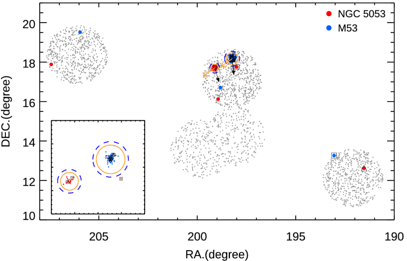
Figure 1: Spatial distribution of all stars in the $20\arcdeg\times 10\arcdeg$ field around M53 and NGC 5053. The subpanel shows the distribution of cluster member candidates inside tidal radii of the clusters. Tidal radii of two clusters ($18.37^{\prime}$ for M53 and $11.43^{\prime}$ for NGC 5053) given by Harris (1996) (2010 edition) are indicated by the orange circles. We also present larger tidal radii of $22.8^{\prime}$ and $15.2^{\prime}$ which are derived by de Boer et al. (2019) as blue dashed circles. The direction toward Galactic center was indicated by orange arrow, and the proper motions of the clusters (Vasiliev, 2019) were represented by black arrow. The points depicted by only blue and red colors are final cluster member candidates in group 1, while the points with open square and triangle are the stars in group 2 and group 3, respectively (see text).

The APOGEE survey provides high resolution (R$\sim$22,500) $H$-band spectra ($\lambda=1.51-1.70\mu m$). The survey delivers two sets of the stellar parameters and chemical abundances for more than 20 elements determined by The Cannon (a data-driven approach to determine stellar parameters and abundances, Ness et al., 2015) and ASPCAP (APOGEE stellar parameters and Chemical Abundances Pipeline, García Pérez et al., 2016). In this work, we use the spectra of APOGEE DR14 (Majewski et al., 2017) and the data catalogue of The Cannon. Our initial sample consists of 2,558 redgiant branch (RGB) stars in the $20\arcdeg\times 10\arcdeg$ field around M53 and NGC 5053 that are covered by the APOGEE survey; the distribution of an initial sample of the sky is shown in Figure 1.

Our approach is to search for stars with spectral characteristics that are similar to the cluster members, where we assume that stars that have decoupled from the clusters will show similar properties in chemical abundances and kinematics to the member stars of the clusters. To measure spectral similarity, we apply t-distributed stochastic neighbor embedding (t-SNE) algorithm to the datasets of chemical abundances and radial velocities. t-SNE is a machine-learning algorithm for visualization with clustering similar features together of the high-dimension data into lower-dimension. It calculates the probability distribution of similarities for each pair of points in the high and low dimensional spaces, respectively, and then tries to find locations in the lower-dimensional space to minimize the difference between these probability distributions (or similarities) for an optimal representation of data points in lower-dimensional space. The Kullback-Leibler (KL) divergence (Kullback & Leibler, 1951), a measure of direct divergence between two probability distributions of overall data points using a gradient descent method, is utilized to measure the difference of probability distributions. A detailed explanation of t-SNE algorithm is described in van der Maaten & Hinton (2008) and Pezzotti et al. (2015) (see their papers for more details). The t-SNE algorithm is now extensively used in astronomy as a classification algorithm (Lochner et al., 2016; Matijevič et al., 2017; Valentini et al., 2017; Traven et al., 2017). In particular,  Anders et al. (2018) and Kos et al. (2018) demonstrated the capability of t-SNE to identify stellar populations in the Milky Way by recognizing the clusters and related field stars, as well as chemically peculiar stars.

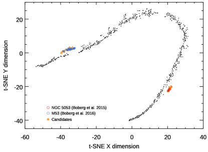
Figure 2: t-SNE projection of stars around M53 and NGC 5053. The points in two subgroups (orange points) at -40 and 20 on the t-SNE X dimension axis are selected cluster member candidates. M53 and NGC 5053 member stars confirmed by Boberg et al. (2015, 2016) are indicated by blue and red open circles, respectively.

We use the t-SNE algorithm included in the scikit-learn python package. As input data for t-SNE, the radial velocity and chemical abundances of The Cannon were used. As different chemical elements have different degrees of uncertainties, we tested several combinations of atomic elements to find the optimal set of elements for our t-SNE analysis. Out of 20 elemental abundances of The Cannon, our analysis is based on 19 elements; Na is excluded because this element is difficult to measure in near-infrared spectra for metal-poor stars. Any stars with poor stellar parameters are not included in the t-SNE computation. Instead, a separate selection process is applied to these stars (described below). Figure 2 shows the t-SNE projection for the stars around M53 and NGC 5053 in Figure 1. The t-SNE projection shows the groups with similar radial velocity and chemical abundances together. One can easily identify that there are two well-defined isolated groups (i.e., the orange dots). It turns out that the group at t-SNE with an X-value of -40 is mostly composed of member stars of M53, while the other group at t-SNE with an X-value of 20 is mostly composed of member stars of NGC 5053. The cluster member stars confirmed by Boberg et al. (2015, 2016) are also well distributed in the two isolated groups. Therefore, we consider all the stars in the two isolated groups as being candidate members of M53 and NGC 5053.

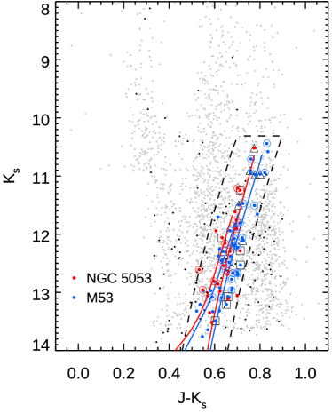
Figure 3: $(J-K_{s},K_{s})$ CMD for the RGB stars around M53 and NGC 5053. The gray dots indicate the all stars in the Figure 1, and black dots are selected member stars from the t-SNE algorithm and those based on the radial velocity criteria (see text). The MIST isochrones with $\mathrm{[Fe/H]=-2.27}$ and $-2.10$ and age of 13 Gyr were plotted as the red and blue solid lines, respectively. The dashed lines are the color and magnitude boundaries for filtering the field stars. Final cluster member candidates in group 1, group 2 and group 3 are represented as Figure 1. The open circles are confirmed cluster member stars recognized in Boberg et al. (2015, 2016).

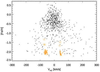
Figure 4: Heliocentric radial velocities versus metallicities of the stars around M53 and NGC 5053 in Figure 1. The cluster member candidates in t-SNE or CMD filtering analysis are indicated by orange dots. The stars in group 2 are indicated by open triangle. Note that five metal-rich stars (orange open circles) were excluded from the final list of the candidates (see text).

In addition to the t-SNE algorithm, we apply separate selection processes. The additional selection processes are used to refine the t-SNE selection and to search for additional member candidates from the sample where we could not apply the t-SNE process due to various reasons (e.g., inaccurate stellar parameters). More specifically, we filter the sample based on the radial velocities, the location in the color-magnitude diagram (CMD), and metallicities $\mathrm{[Fe/H]}$. These filtering processes are guided by properties of known cluster members and the t-SNE selected candidates.

For the baseline criteria, we select stars with a radial velocity range of about $\pm 15$ km s^-1 from the mean value of the two clusters, $V_{rad}=44$ km s^-1 for NGC 5053 (Pryor et al., 1991; Geisler et al., 1995; Yan & Cohen, 1996, adopted from  Harris, 1996) and $V_{rad}=-63$ km s^-1 for M53 (Lane et al., 2010, adopted from  Harris, 1996). We further apply filtering based on their location of the CMD. Figure 3 shows the $(J-Ks,Ks)$ CMD of all stars (gray dots) in Figure 1 and the stars (black dots) filtered by the radial velocities criteria. The filtering criteria for the CMD (dashed lines in Figure 3) is determined by considering the theoretical isochrones of the clusters and the distribution of confirmed and t-SNE selected cluster members. The isochrones are derived from MIST (Choi et al., 2016; Dotter, 2016) for $\mathrm{[Fe/H]=-2.10}$ and $-2.27$ and age of 13 Gyr that are relevant to M53 and NGC 5053. With respect to these isochrones, we define our selection boundary with the color-width of about 0.1 mag and a magnitude range of $K_{s}=10.3\sim 14.0$, which comfortably enclose all the confirmed cluster members (Boberg et al., 2015, 2016). We note that, among the t-SNE selected candidates, three stars were outside of this boundary, and they are dropped from our candidate sample.

Finally, we apply criteria for $\mathrm{[Fe/H]}$. Figure 4 shows the distributions of $\mathrm{[Fe/H]}$ and the heliocentric radial velocity for our initial sample, together with the member candidates selected from the t-SNE or CMD filtering process. In addition to radial velocity, the member candidates show reasonable metallicity distribution that is consistent with the metallicities of clusters from previous studies. We also find a few member candidates show relatively a high value of metallicity greater than $\mathrm{[Fe/H]=-1.8}$. While we are inclined to drop these stars of high metallicity, we want to be careful, as several studies based on the APOGEE catalogue have reported possible systematic bias in their metallicity at a low metallicity ($\mathrm{[Fe/H]<-1.0}$) domain. As a cautionary measure, we conduct our own spectral synthesis analysis to independently derive metallicity and chemical abundances (details are described in Section 4). We assign metallicity range for cluster member candidates with $-2.3<\mathrm{[Fe/H]}<-1.8$ for M53; and $-2.45<\mathrm{[Fe/H]}<-1.85$ for NGC 5053. These are determined from the mean metallicities and the standard deviations from our own analysis. The candidate stars of high metallicity from the APOGEE catalog resulted in similarly high metallicity, based on our analysis. Thus, the five stars with high metallicity are removed from the cluster candidates.

Table 1: Number of selected cluster member (and extra tidal star) candidates and selection method

Group	M53	NGC 5053	Selection method
			t-SNE	CMD	$V_{HC}$	[Fe/H]
Group 1	40 (2)	18 (2)	O	O	O	O
Group 2	5 (1)	3 (1)	X	O	O	O
Group 3	6 (0)	1 (1)	X	O	O	X
total	51 (3)	22 (4)	-	-	-	-

Table 2: Selection creteria

Method	M53	NGC 5053
t-SNE (X)	-40	20
CMD ($J-K_{s}$)	0.45 $\sim$ 0.90	0.45 $\sim$ 0.90
$(K_{s})$	10.3 $\sim$ 14.0	10.3 $\sim$ 14.0
$V_{HC}$ (km/s)	-78.2 $\sim$ -48.2	30.1 $\sim$ 60.1
$[$Fe/H$]$ (dex)	-2.3 $\sim$ -1.8	-2.45 $\sim$ -1.85

We finally identify $73$ stars (51 for M53 and 22 for NGC 5053) as being cluster member candidates. Note that 33 and 13 stars are cross-matched with sample stars of Boberg et al. (2015, 2016) for M53 and NGC 5053, respectively. We classify them into three groups based on the likelihood of membership. All the candidates conform to our CMD criteria. Group 1 represents candidates that are most likely selected via t-SNE and also conform to our radial velocity and metallicity criteria. Group 2 represents candidates that conform to the radial velocity and metallicity criteria, but for which t-SNE was not applicable. Group 3 are candidates filtered by radial velocity criteria only, as neither t-SNE nor metallicity cut is applicable given the poor spectral quality. The member candidates in Group 1, Group 2 and Group 3 are represented as colored points, open squares, and open triangles in Figure 1 and Figure 3. In Table 1, we summarize the number of cluster member stars in each group and indicate applied selection methods. The number in parentheses indicates the number of extra-tidal stars. In Table 2, the selection criteria for each selection method are indicated.

3 Spatial distribution and extra-tidal stars from the clusters

In Figure 1, we show the spatial distribution of our 73 cluster member candidates in the sky. Member candidates of M53 are marked with blue points, and those of NGC 5053 are marked with red. Also shown are the tidal radii of each cluster. In this study, we derive the tidal radii of M53 and NGC 5053 using the structural parameters (core radius and central concentration) in Harris (1996, 2010 edition), which are actually derived by the King model fitting to the radial density profiles of clusters (Lehmann & Scholz, 1997). The calculated tidal radii are $18.37^{\prime}$ for M53 and $11.43^{\prime}$ for NGC 5053. We are certain that the derived tidal radii are appropriate for describing the limit of the clusters. The radial density profiles of M53 and NGC 5053 in Chun et al. (2010) showed that overdensity features with clear slope changes in the profile that depart from the King model start at $15^{\prime}$ and $10^{\prime}$, respectively, and extend to $34^{\prime}$ from the cluster center. The tidal radius is entirely dependent on the fitting model, and indeed larger tidal radii of $22.8^{\prime}$ and $15.2^{\prime}$ for M53 and NGC 5053, respectively, were reported by de Boer et al. (2019). Using the data of Gaia DR2, they fitted a Spherical Potential Escapers Stitched (SPES) model which shows a more detailed description of stars at the escape energy to the density profile of the clusters. We note that adopting larger tidal radii does not change the final results, because identified extra-tidal stars are still beyond the larger tidal radii. In Figure 1, we present the larger tidal radii by de Boer et al. (2019) as dashed blue circles.

We see most of the candidates are indeed located within the tidal radii of the clusters. We do not see any obvious tidal extension of candidates, but given the small number of samples, we do not expect to see one, even if there is one present. It is apparent, however, that several member candidates are located well beyond the tidal radii. We find a total of seven possible extra-tidal stars; three stars out of the 51 candidates of M53 members, and four out of the 22 of NGC 5053. Among seven likely extra-tidal stars, four are from Group 1, two are from Group 2, and one is from Group 3 (see Table 1). We note that  Tang et al. (2018) recently investigated the stars of NGC 5053 using the same APOGEE data that we used, but they were not able to identify any extra-tidal star. They only considered the stars within three times the tidal radius of NGC 5053, and all our candidates are located beyond their search radius. The most distant extra-tidal stars of M53 and NGC 5053 are more than 8 degree away from the cluster. At this large scale, our initial search sample is strongly biased by the coverage of the APOGEE survey, which is obvious from Figure 1. Given a small number of extra-tidal candidates and very small coverage of the initial samples, we are limited in investigating the spatial distribution of extra-tidal stars. However, in the vicinity of two clusters within a few degrees from the clusters, there are some notable aspects in the distribution.

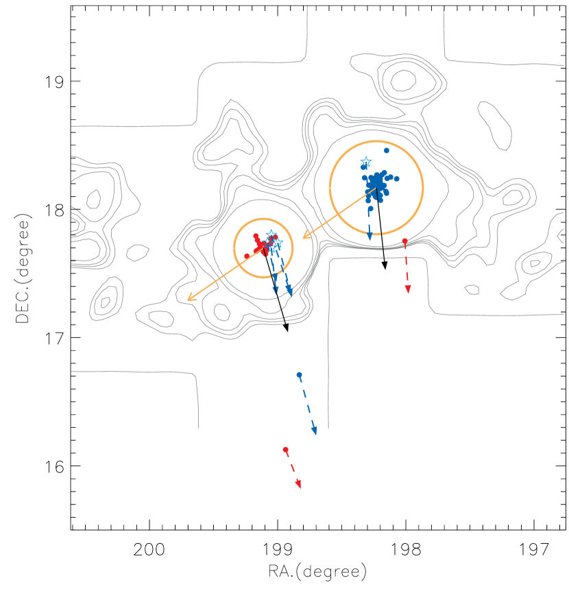
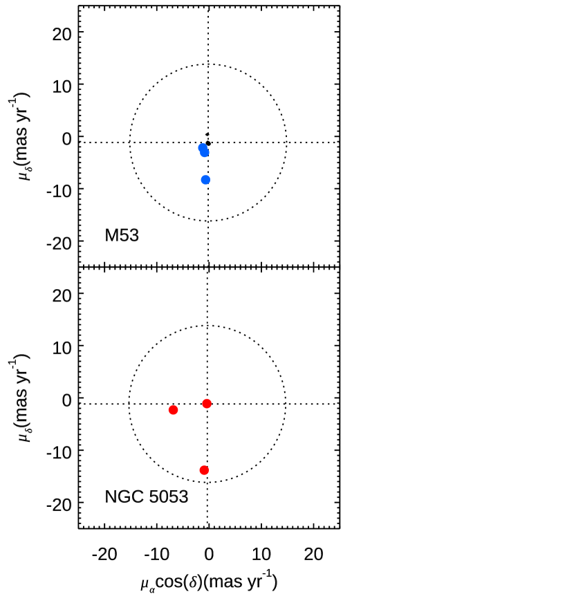
Figure 5: Left: Expansion of spatial distribution of stars near the two clusters with isodensity contour map of Chun et al. (2010). The tidal radii of clusters are indicated by orange circles. The direction toward the Galactic center and proper motion of the clusters are represented by orange and black arrows, respectively. The dotted arrows are the proper motion (Gaia Collaboration et al., 2018, Gaia DR2) direction for extra-tidal stars. The blue points are for cluster member candidates of M53 and red points are for NGC 5053. Five extra-tidal RR Lyrae stars of M53 from Kundu et al. (2019) are also plotted by open stars. Right: Proper motion diagram of extra-tidal stars. The intersection of dotted line is nominal proper motion of the cluster (Vasiliev, 2019).

The left panel of Figure 5 shows the zoomed-in view of the spatial distribution centered around the two clusters. Overlaid are the stellar density contours around M53 and NGC 5053 from Chun et al. (2010). In addition to the member candidates from this work, we overplot the extra-tidal RR Lyrae stars of M53 of Kundu et al. (2019). The solid black arrows indicate the proper motion of M53 and NGC 5053. The proper motions of individual extra-tidal star candidates, if available from the Gaia DATA Release 2, are indicated by dotted arrows. They all show similar proper motion to their suggested parental clusters. The right panel of Figure 5 shows the proper motion diagram of six stars in our seven extra-tidal stars, and the proper motions are consistent with those of the suggested parental clusters (within about $15$ mas yr^-1, dotted circle). It is also notable that three extra-tidal star candidates from this work are located along the leading direction of the cluster proper motion.

The stellar density contour of Chun et al. (2010), and their possible association with extra-tidal candidates can be interesting. However, the stellar density contours of Chun et al. (2010) are limited in their coverage; thus, it is not trivial to associate the features in the density contours to the location of extra-tidal candidates. Even with these limitations, it is notable that there are small clumps along the trailing direction of the cluster proper motion and on the extension line between the extra-tidal candidates and the clusters. Marginal density contours also seem to approach or bend toward extra-tidal stars. We note that tidal tails or extra-tidal stars should be aligned with the cluster’s orbit (Combes et al., 1999; Dehnen et al., 2004; Jordi & Grebel, 2010; Eyre & Binney, 2011), but extra-tidal stars located in different positions from the cluster do not need to have similar proper motion (e.g., Anguiano et al., 2016). Therefore, several properties of extra-tidal stars, such as the alignment toward the leading direction of the cluster proper motion, similar proper motions, and marginal association with stellar density contour, support the idea that these stars are extra-tidal stars decoupled from two globular clusters.

Two other interesting features in stellar density contour of Chun et al. (2010) are the tidal bridge feature and the tidal common envelope between the two clusters.  Chun et al. (2010) suggested dynamical interaction between clusters. In this regard, it is interesting to note that one of the extra-tidal stars of NGC 5053 $(\alpha,\delta)\sim(198.0,17.8)$ is indeed located within the M53 side of the common envelope, which raises the interesting possibility that this star was originally a member of NGC 5053, was stripped from its initial prenatal cluster, and is now under the gravitational influence of M53.  Kundu et al. (2019) reported five extra-tidal RR Lyrae stars of M53 from Gaia DR2, and we find that four of them are located inside the tidal radius of NGC 5053 and have very similar proper motion to that of M53. This may provide another piece of evidence that the two clusters are dynamically interacting and possibly swapping their member stars. However, we are concerned that the four extra-tidal RR Lyrae stars of Kundu et al. (2019) are simply member stars of NGC 5053. Since M53 and NGC 5053 show similar proper motion and have similar apparent magnitude, accidentally misidentification of the member stars of NGC 5053 as extra-tidal sources of M53 is sufficiently possible. Indeed, Ngeow et al. (2020) recently reported that the four extra-tidal RR Lyrae stars identified by Kundu et al. (2019) were already-known RR Lyrae stars of NGC 5053 in the “Updated Catalog of Variable Stars in Globular Clusters” (Clement et al., 2001; Clement, 2017). Therefore, we consider these RR Lyrae stars as being the member stars of NGC 5053, not extra-tidal stars of M53. Note that the radial velocity of these stars and the period-luminosity-metallicity relation of RR Lyrae in the two clusters are helpful for further discussion.

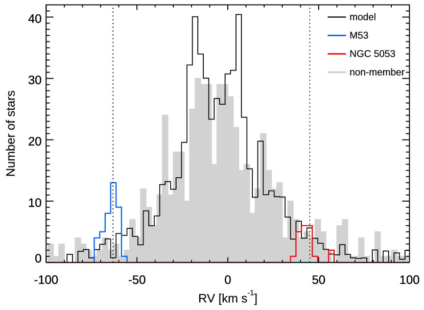
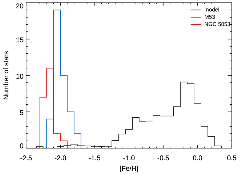
Figure 6: Left: Radial velocity distribution for observed stars and model populations. Blue and red histograms are radial velocity distribution of M53 and NGC 5053, respectively. The dotted lines are nominal radial velocities of the clusters. The observed cluster non-member are overplotted by grey histogram. Right: Metallicity distribution of cluster member stars and model populations

To investigate possible contamination by field stars to our sample of cluster member candidates, we use the Besançon Galaxy model (Robin et al., 2003) to simulate the radial velocity and metallicity distribution of field stars. We generate 100 Galaxy models covering the same areas around the clusters. We then apply the same selection criteria we used for the membership selection in the CMD space (i.e., the dashed lines in Figure 3). Figure 6 shows the radial velocity (left panel) and metallicity (right panel) distribution of the simulated stars. Radial velocity distribution is normalized to the total number of observed non-member stars, while the metallicity distribution is normalized to the total number of cluster member stars. The distributions for the cluster members are indicated by the blue (M53) and red (NGC 5053) histograms. We note that the metallicities of the clusters in Figure 6 are from our own analysis, which will be described in Section 4.

In the radial velocity distribution, we find that the mean velocities of the stars designated as cluster members are $-63.2\pm 4.1$ km s^-1 for M53, and $45.1\pm 5.3$ km s^-1 for NGC 5053. These mean radial velocities are in agreement with the previously derived values of $-63.2\pm 0.5$ km s^-1 for M53 (Boberg et al., 2016), and $42.0\pm 1.4$ km s^-1 for NGC 5053 (Boberg et al., 2015). Unfortunately, it is apparent that the radial velocity distributions of cluster stars are not much different from the Galaxy model distribution. M53 distribution shows a peak at its mean velocity, but this does not seem to be dominant, compared to the model distribution. A Kolmogorov-Smirnov (KS) test for the null hypothesis that observed radial distributions of the clusters and the model come from the same distribution also provides $p$-values of about $P=0.07$ for M53, and $P=0.37$ for NGC 5053; this indicates that we cannot reject the null hypothesis. On the other hand, metallicity distributions of the clusters and the Galaxy model show an interesting feature. The Galaxy model predicts fewer than one star of such low metallicity ($\mathrm{[Fe/H]\sim-2.0}$) in the cluster field. However, the metallicity distributions of two clusters show apparent and prominent peaks at low metallicities. The $p$-values of the KS test to compare the cluster and model metallicities are also almost zero ($7.64\times 10^{-34}$ for M53, and $1.06\times 10^{-18}$ for NGC 5053). It is unlikely that the observed and expected metallicity distributions come from the same parent distribution. In addition, we search for the stars from the Galaxy model that are consistent with our criteria for member candidates (i.e., based on metallicity and radial velocity criteria), and we find that only two field stars are in this condition. Based on a comparison with the Galaxy model, the radial velocities of the identified cluster and extra-tidal stars are consistent with those predicted by the Galaxy model, even though our sample stars are clearly different populations from the Galaxy populations in terms of metallicity. There are only two halo interlopers, which are consistent with both the radial and the metallicity criteria of the member candidates. Therefore, our extra-tidal stars are likely associated with the two globular clusters, even though we cannot definitively exclude the possibility that they are normal field stars.

4 Chemical properties of clusters and extra-tidal stars

The anomalies of light-elements, such as C, N, O, F, Na, Al, Mg and Si, are unique features that are found only in globular clusters; thus, the Galactic field stars with light-element patterns similar to those seen in second-populations of the globular clusters are considered to be escaped stars from the globular clusters. Indeed, several studies have reported the Galactic field stars with GC-like abundance patterns and discussed the association thereof with globular clusters (e.g., Ramírez et al., 2012; Wylie-de Boer et al., 2012; Carretta, 2013; Martell et al., 2016; Schiavon et al., 2017). Therefore, if our extra-tidal candidate stars show GC-like abundance patterns, a physical association with the clusters will be strongly supported. Many previous studies (Mészáros et al., 2015; Jönsson et al., 2018; Tang et al., 2018; Masseron et al., 2019) have suggested that the chemical abundances for metal-poor stars ($\mathrm{[Fe/H]}<-1.0$) provided by the APOGEE pipeline may exhibit systematic offset. Thus, we reanalyze the APOGEE spectra of the cluster member candidates and manually estimate their chemical abundances. We focus on atomic elements Mg, Al, and Si, because their spectral lines are relatively prominent in the APOGEE spectra for metal-poor stars. We investigate abundance anomalies for these elements, as well as the chemical association of extra-tidal stars with the clusters.

4.1 Stellar parameters and synthetic fitting

To estimate the chemical abundances for the clusters and extra-tidal stars, we photometrically calculate the stellar atmospheric parameters. Using the relations of González Hernández & Bonifacio (2009), the effective temperatures ($T_{\mathrm{eff}}$) are derived from broadband $B,V$ (Boberg et al., 2015, 2016) and 2MASS $J,H,K$ (Skrutskie et al., 2006) photometries. The reddening correction is applied with $E(B-V)=0.018$ for M53 and $E(B-V)=0.015$ for NGC 5053 (Schlafly & Finkbeiner, 2011). The values of $T_{eff}$ obtained from $B-V$, $V-J$, and $J-K$ are averaged and adopted as final $T_{\mathrm{eff}}$, or those from $J-K$ are chosen for the stars with only $J-K$ color. The surface gravities are calculated from the following relation:

$$\log{g}=\log{g_{\odot}}+\log\left(\frac{M_{\star}}{M_{\odot}}\right)+4\log\left(\frac{T_{\mathrm{eff\star}}}{T_{\mathrm{eff\odot}}}\right)+0.4(M_{bol,\star}-M_{bol,\odot}).$$ (1)

The solar values of $\mathrm{log}$ $g_{\odot}=4.438$, $M_{bol.\odot}=4.75$, and $T_{eff,\odot}=5772$ K  (Prša et al., 2016) are used, and we assume a mass of $0.8M_{\odot}$ for our sample stars. The bolometric correction (BC) values are estimated from the relation between BC values and $J-K$ color of Montegriffo et al. (1998). Distance moduli of $(m-M)_{V}=16.32$ for M53, and $(m-M)_{V}=16.23$ for NGC 5053  (Kopacki, 2000; Arellano Ferro et al., 2010, adopted from Harris, 1996) are used. The equation $v_{t}=\mathrm{2.24-0.3\times log}$ $g$ from Mészáros et al. (2015) is then used to calculate micro-turbulence velocity ($v_{t}$). Table 3 shows the sample of derived stellar parameters.

Table 3: Stellar parameters, metallicity, and abundances of M53 and NGC 5053

2MASS ID	$T_{\mathrm{eff}}$	log $g$	$v_{t}$	[Fe/H]	$\sigma_{[Fe/H]}$	[Mg/Fe]	$\sigma_{[Mg/Fe]}$	[Al/Fe]	$\sigma_{[Al/Fe]}$	[Si/Fe]	$\sigma_{[Si/Fe]}$	Cluster
2M13434835+1931084	4836	1.10	1.91	-2.051	0.020	0.500	0.025	-0.029	0.060	0.393	0.072	M53
2M13151955+1642373	4656	1.36	1.83	-2.223	0.088	0.482	0.096	-0.138	0.090	0.449	0.090	M53
2M13123617+1827323	4634	1.58	1.77	-2.013	0.019	0.512	0.019	-0.037	0.029	0.509	0.027	M53
2M13124987+1811487	4647	1.39	1.82	-1.908	0.100	0.289	0.106	-0.419	0.105	0.321	0.114	M53
2M13124768+1810060	4421	0.96	1.95	-2.012	0.080	0.310	0.105	1.101	0.085	0.482	0.083	M53
2M13130945+1811188	4678	1.36	1.83	-1.985	0.025	0.439	0.059	0.801	0.039	0.495	0.036	M53
2M13121714+1814178	4558	1.48	1.79	-1.972	0.075	0.393	0.084	-0.135	0.083	0.343	0.076	M53
2M13124082+1811099	4672	1.64	1.75	-2.084	0.016	0.512	0.017	0.993	0.052	0.600	0.038	M53
…	…	…	…	…	…	…	…	…	…	…	…	…
2M13120179+1745121	4769	1.27	1.86	-2.182	0.044	0.505	0.054	-0.073	0.046	0.559	0.047	NGC 5053
2M13154512+1607370	4799	1.64	1.75	-2.141	0.123	0.405	0.126	0.199	0.159	0.483	0.130	NGC 5053
2M13493976+1753033	4861	1.23	1.87	-2.103	0.054	0.257	0.114	-0.003	0.114	0.496	0.106	NGC 5053
2M13161223+1746228	4464	0.91	1.97	-2.174	0.016	0.271	0.016	0.270	0.101	0.291	0.053	NGC 5053
2M13160457+1747017	4684	1.69	1.73	-2.322	0.072	0.223	0.088	0.942	0.123	0.442	0.073	NGC 5053
2M13162073+1741059	4738	1.51	1.79	-2.109	0.021	0.067	0.077	0.907	0.102	0.395	0.077	NGC 5053
2M13162226+1741536	4850	1.42	1.81	-2.193	0.029	0.219	0.052	1.038	0.104	0.648	0.030	NGC 5053
2M13162059+1742464	4560	1.14	1.90	-2.196	0.032	0.328	0.084	0.040	0.105	0.268	0.087	NGC 5053
…	…	…	…	…	…	…	…	…	…	…	…	…

Based on the derived stellar parameters, we estimate chemical abundances of individual elements (i.e., Fe, Mg, Al, and Si) by synthetic spectral fitting to the interesting atomic lines in the observed spectra. The synthetic spectra are generated by Turbospectrum (Alvarez & Plez, 1998; Plez, 2012) with the atmospheric models interpolated from MARCS model grid (Gustafsson et al., 2008), and the internal APOGEE DR14 atomic/molecular linelist (linelist 20150714) is used in the model calculation. The calculated synthetic spectra are then convolved by a line-spread function (LSF) that is used in ASPCAP to match the observed line profile and the spectral resolution. Based on the atomic wavelength regions of Smith et al. (2013) and  Afsar et al. (2018), we visually inspect several prominent atomic lines and compare them with synthetic spectra of which chemical abundances are adjusted to match observed spectra. In order to avoid spurious results, the atomic lines that are very weak or significantly blended by other lines are rejected. The best matched spectrum with a minimum $\chi^{2}$-value between the synthetic and the observed spectra is determined. The average of individual measurements and the standard deviation are decided as the final chemical abundances and errors. The estimated metallicities and abundances of Mg, Al, and Si are summarized in Table 3 with respect to the solar abundances from Asplund et al. (2009).

Calculated abundances are significantly affected by the uncertainty of atmospheric parameters. Therefore, we comapre our atmospheric parameters with previous results of others, and quantify the abundance variation due to the parameter changes. Following the standard deviation of temperature relation of González Hernández & Bonifacio (2009), the typical uncertainty in $T_{\mathrm{eff}}$ ($\Delta T$) is about $\sim 100$ K, which leads average uncertainties in log $g$ and $v_{t}$ of $\pm 0.05$ dex and $0.02$ km s^-1, respectively.

We first compare our atmospheric parameters with those of Boberg et al. (2015, 2016) for the cross-matched stars in M53 and NGC 5053. The $T_{\mathrm{eff}}$ of Boberg et al. (2015, 2016) was calculated from the Alonso relation (Alonso et al., 1999). We find that the difference in $T_{\mathrm{eff}}$ with  Boberg et al. (2015, 2016) is about $\sim 70$ K hotter with a standard deviation of 50 K, and only a few stars are hotter by $\sim 150$ K. The average differences in log $g$ and $v_{t}$ are small; $0.08$ $(\sigma=0.12)$ dex and $0.04$ $(\sigma=0.17$) km s^-1, respectively. We note that the uncertainties of atmospheric parameters of Boberg et al. (2015, 2016) are 100 K in $T_{\mathrm{eff}}$, 0.2 dex in log $g$, and 0.25 km s^-1 in $v_{t}$, which indicates that the adopted atmospheric parameters in this study are consistent with previous parameters within the error range.

We then investigate the sensitivity of abundances due to the variations in adopted atmospheric parameters. Abundances are re-estimated with new synthetic models, which are calculated by varying atmospheric parameters (temperature, gravity, and microturbulence) one by one. The parameter changes are the uncertainties in the parameters (i.e., $\Delta T=100$ K, $\Delta\mathrm{log}$ $g=0.05$, and $\Delta v_{t}=0.02$ km s^-1). Table 4 shows the mean sensitivity of abundances according to the atmospheric parameters changes. The variation of atmospheric parameters results in a total uncertainty of about 0.1 dex in abundances; the effective temperature uncertainties are the main contribution of the abundance uncertainties.

Table 4: Sensitivity of abundances due to variation of atmospheric parameters

Element	$\Delta T_{\mathrm{eff}}(\pm 100K)$	$\Delta$ log $g$ ($\pm$0.05)	$\Delta v_{t}(\pm$0.02)
Fe	$\pm 0.07$	$\mp 0.07$	$\pm 0.03$
Mg	$\pm 0.08$	$\mp 0.01$	$\pm 0.01$
Al	$\pm 0.08$	$\mp 0.01$	$\pm 0.02$
Si	$\pm 0.09$	$\pm 0.05$	$\pm 0.03$

4.2 Abundance results

From the manual abundance analysis, metallicities and elemental abundances of 73 cluster member candidates were investigated. Excluding stars with poor spectral quality, reliable estimates of metallicities and abundances of 65 stars (44 stars for M53 and 21 stars for NGC 5053) were obtained, including six out of seven extra-tidal stars. The average metallicities of M53 and NGC 5053 are [Fe/H]=-2.00$\pm$0.10 and [Fe/H]=-2.17$\pm$0.07, which agrees with the metallicities that were previously reported by Harris (1996). Here, we note that the 21 sample stars of NGC 5053 is the largest sample for which chemical abundances have been investigated in near-infrared high-resolution spectroscopy for this metal-poor cluster.

The left panel of Figure 7 shows the distribution of Al abundances as functions of Mg for the cluster stars. It is apparent that there are clear Mg-Al anticorrelations for M53 and NGC 5053. Al abundances of M53 show a large spread of about 1.0 dex, while those of NGC 5053 are about 0.8 dex. We also found a clear gap in the Al distribution, which indicates that the populations of M53 and NGC 5053 are separated into two distinct abundance groups (i.e., Al-depleted first generation and Al-enhanced second generation). The extremely Mg-depleted stars ([Mg/Fe]$<$0), which are commonly detected in the most metal-poor globular clusters, such as M15 and M92 (Masseron et al., 2019), are not found in our clusters. Instead, the distribution of Mg abundance shows no strong variation for each cluster. Mg-Al anticorrelation in globular clusters (including M53) has already been reported in many studies (e.g., Carretta et al., 2009; Mészáros et al., 2015; Masseron et al., 2019). Thus, we directly compared our results of M53 with those of Masseron et al. (2019), and found similar Mg-Al anticorrelation with almost the same Al abundance spread range. However, the prominent Mg-Al anticorrelation of NGC 5053 studied in this study has never been investigated. A light symptom of Na-O and Mg-Al anticorrelation was reported (Boberg et al., 2015; Tang et al., 2018) for the very limited samples of NGC 5053. We found more first-generation stars of NGC 5053 near and below the upper limit of Al abundance by Tang et al. (2018), which enabled us to find a clear Al variation in NGC 5053.

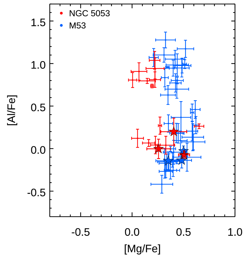
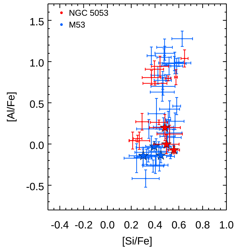
Figure 7: Al abundances as function of Mg (left panel) and Si (right panel) abundances for cluster member stars. The blue and red points are the stars of M53 and NGC 5053, respectively. The six extra-tidal stars are described by five point star marks. There is a clear Mg-Al anticorrelation for the stars of both clusters. The Al-Si plane shows the light Al-Si correlation.

The Al-Si distribution of the two clusters is plotted in the right panel of Figure 7. Our sample size of NGC 5053 is large enough and clearly confirms the Si spread in this cluster that was previously reported by Tang et al. (2018). We found a light variation ($\sim 0.3$ dex) in Si abundance for NGC 5053, which caused a light Al-Si correlation, while the Si abundance seemed to have a constant value for M53. The Al-Si correlation was the result of ${}^{28}\mathrm{Si}$ leakage from the Mg-Al chain (Yong et al., 2005; Carretta et al., 2009; Mészáros et al., 2015). This nuclear reaction requires a very high temperature of $\sim 80$ MK (Prantzos et al., 2017), for which low-metallicity clusters or massive clusters are preferable. The low-metallicity clusters M15 and M92 show an apparent Al-Si correlation with a significant Si variation (Mészáros et al., 2015; Masseron et al., 2019). NGC 5053 is also one of the most metal-poor clusters in the Milky Way with a metallicity comparable to those of M15 and M92, even though its cluster mass is less massive. Therefore, a similar Si distribution of NGC 5053 to that of M15 and M92 is not surprising. It is interesting that the less metal-poor but more massive cluster M53 does not show Si variation. In this respect, the different extents of Mg, Si, and Al variations in M53 and NGC 5053 indicates that metallicity is not the only factor that regulates the correlation between the light elements.

5 Discussion and conclusion

From the manual chemical analysis, Mg, Al, and Si abundances of six extra-tidal stars were reliably estimated. We found that the identified extra-tidal stars had similar chemical properties with cluster stars (see Figure 7), and they were all located in the low Al abundance region (i.e., first-generation of the clusters). The Mg-rich/Al-poor feature of extra-tidal stars indicates that they could be the field stars that originated from first-generation populations of the clusters. In globular clusters, first-generation stars are less centrally concentrated than second-generation stars (Lardo et al., 2011), making them more vulnerable to tidal interaction. Thus, it is not surprising that most extra-tidal stars are first-generation stars.

The origin of multiple populations in globular clusters is still being debated, and no single model can successfully explain all the observational results. Still, a common prediction among different models (e.g., Decressin et al., 2007; D’Ercole et al., 2008; Ventura & D’Antona, 2008; Bastian et al., 2013; Bastian & Lardo, 2018) is that globular clusters were initially much more massive than currently observed, and a large fraction of stars have been lost since their formation. Some models suggest that globular clusters were 25 times more massive than present and lost as much as 90 $\%$ of their stars. Other studies (Kruijssen, 2015; Baumgardt, 2017; Baumgardt & Sollima, 2017; Baumgardt et al., 2019) suggest that initial globular clusters are 4$\mathrm{-}5$ times larger and average star loss is about $75\mathrm{-}80\mathrm{\%}$. We note that recent studies (Vesperini et al., 2010; Larsen et al., 2012; Milone et al., 2017; Schiavon et al., 2017) have indicated that heavy mass loss of up to 90 $\%$ is unrealistic and presents several problems (Bastian & Lardo, 2015), and that about 50 $\%$ mass loss seems more acceptable. In this case, at least about 10 $\%$ of the Galactic halo stars could have originated from globular clusters (Martell et al., 2016; Koch et al., 2019). Recently,  Hanke et al. (2020) investigated the chemodynamical association of the halo stars with globular clusters, and suggested that the fraction of first-generation cluster stars among all stars escaped from clusters into the halo is about 50$\%$ in the vicinity of the clusters and 80$\%$ in the distant halo field. Therefore, we propose that the extra-tidal stars that we found in this work were first-generation stars in M53 and NGC 5053 that became unbound from their parental clusters.

In this study, we found 73 cluster member candidates of two globular clusters, M53 and NGC 5053, using the t-SNE algorithm, radial velocity, and a manual chemical abundance analysis. Out of those, seven stars were beyond the tidal radii of two clusters and were thus likely to be extra-tidal stars associated with either M53 or NGC 5053. The extra-tidal stars in the vicinity of the clusters appeared to share the proper motion direction with those of the clusters. Furthermore, small clumps in stellar density contour of Chun et al. (2010) and these stars were well-aligned along the trailing and leading direction of cluster proper motion. The morphology of distortion in marginal stellar density contour seems to approach these stars. A chemical abundance analysis for extra-tidal stars showed that these stars could be first-generation stars stripped from the two clusters by tidal disruption or tidal interaction between the clusters.

It is notable that one extra-tidal star of NGC 5053 is in the M53 side of the common envelope of Chun et al. (2010). This may represent the stars that were tidally stripped and gravitated toward its neighbor, and it may serve as a direct evidence that two clusters experienced dynamical interaction, although the radial velocities are different by 105 km s^-1. A tidal link between the two clusters could indicate that these clusters did not originate from the Milky Way, but from dwarf galaxies, as the interaction between the clusters would have occurred more preferentially in dwarf galaxies (van den Bergh, 1996).  Mackey & Gilmore (2004) noted that M53 is an accreted cluster.  Vasiliev (2019) used 6d phase space information of all the globular clusters in the Milky Way from GAIA data and found that M53 and NGC 5053 have very similar dynamical structures together with several more globular clusters, (i.e., similar total energy, orbit and z-component angular momentum), which infers the possible accretion origin thereof from the dwarf galaxy. The Sgr dwarf galaxy was not their progenitor, as it shows a significantly different orbit from those of clusters (Sohn et al., 2018; Tang et al., 2018). More recently,  Massari et al. (2019) investigated the origin of globular clusters and tried to link the known merging or accretion events in the Milky Way using the same 6d phase space information; they further suggested that M53 and NGC 5053 belong to the Helmi streams (Helmi et al., 1999).

In this respect, finding more extra-tidal stars that could reflect tidal interaction between the clusters, especially in the tidal bridge or common envelope of Chun et al. (2010), is important to better understand the dynamical evolution of these clusters. Four extra-tidal RR Lyrae stars of M53 (Kundu et al., 2019) located inside the tidal radius of NGC 5053 could be of interest, but we are certain that these stars are the member stars of NGC 5053, as reported by Ngeow et al. (2020).  Ngeow et al. (2020) searched for additional RR Lyrae stars in the vicinity of the two clusters, and concluded that there are no extra-tidal RR Lyrae stars associated with either M53 or NGC 5053. However, we still expect that the near-field surrounding these clusters has the potential to find more extra-tidal stars. The present RR Lyrae stars in the clusters had been more massive than RGB and main-sequence stars, while the low mass stars are more easily affected by a tidal stripping event or tidal interaction. The APOGEE stars explored in this study are also very bright RGB stars in the two clusters. Therefore, the detection of our extra-tidal RGB stars with a bright magnitude increases the possibility of finding more extra-tidal stars with a fainter magnitude.

In summary, we note that additional photometry and spectroscopy studies for these clusters and the surrounding stars are required to find more definitive evidence of the tidal disruption and the tidal interaction between them. Since RGBs only make up a small percentage of the stellar populations in globular clusters, it is necessary to search for any tidal substructures of more numerous populations, such as main-sequence stars. We note that the most populations that comprise the stellar substructures around M53 and NGC 5053 detected by Chun et al. (2010) are, indeed, main-sequence stars. Homogeneous deep and wide photometry data could provide a finer morphology of stellar substructures to infer the tidal disruption and a possible link between the clusters. The follow-up spectroscopic data of SDSS-V (Kollmeier et al., 2019), 4MOST (Christlieb et al., 2019; Helmi et al., 2019), and MOONS (Cirasuolo et al., 2012) for fainter stars than APOGEE samples could also provide more reliable chemical associations for extra-tidal stars in the substructures of the clusters. Numerical simulations of binary star clusters are also essential to understand the kinematics of tidally stripped stars by neighboring clusters.

References

- Af\textcommabelowsar et al. (2018) Af\textcommabelowsar, M., Sneden, C., Wood, M. P., et al. 2018, ApJ, 865, 44
- Alonso et al. (1999) Alonso, A., Arribas, S., & Martínez-Roger, C. 1999, A&AS, 140, 261
- Alvarez & Plez (1998) Alvarez, R., & Plez, B. 1998, A&A, 330, 1109
- Anders et al. (2018) Anders, F., Chiappini, C., Santiago, B. X., et al. 2018, A&A, 619, A125
- Anguiano et al. (2016) Anguiano, B., De Silva, G. M., Freeman, K., et al. 2016, MNRAS, 457, 2078
- Arellano Ferro et al. (2010) Arellano Ferro, A., Giridhar, S., & Bramich, D. M. 2010, MNRAS, 402, 226
- Asplund et al. (2009) Asplund, M., Grevesse, N., Sauval, A. J., & Scott, P. 2009, ARA&A, 47, 481
- Bastian et al. (2013) Bastian, N., Lamers, H. J. G. L. M., de Mink, S. E., et al. 2013, MNRAS, 436, 2398
- Bastian & Lardo (2015) Bastian, N., & Lardo, C. 2015, MNRAS, 453, 357
- Bastian & Lardo (2018) —. 2018, ARA&A, 56, 83
- Baumgardt (2017) Baumgardt, H. 2017, MNRAS, 464, 2174
- Baumgardt et al. (2019) Baumgardt, H., Hilker, M., Sollima, A., & Bellini, A. 2019, MNRAS, 482, 5138
- Baumgardt & Makino (2003) Baumgardt, H., & Makino, J. 2003, MNRAS, 340, 227
- Baumgardt & Sollima (2017) Baumgardt, H., & Sollima, S. 2017, MNRAS, 472, 744
- Beccari et al. (2008) Beccari, G., Lanzoni, B., Ferraro, F. R., et al. 2008, ApJ, 679, 712
- Bellazzini et al. (2003) Bellazzini, M., Ferraro, F. R., & Ibata, R. 2003, AJ, 125, 188
- Belokurov et al. (2006) Belokurov, V., Zucker, D. B., Evans, N. W., et al. 2006, ApJ, 642, L137
- Boberg et al. (2015) Boberg, O. M., Friel, E. D., & Vesperini, E. 2015, ApJ, 804, 109
- Boberg et al. (2016) —. 2016, ApJ, 824, 5
- Carretta (2013) Carretta, E. 2013, A&A, 557, A128
- Carretta et al. (2009) Carretta, E., Bragaglia, A., Gratton, R., & Lucatello, S. 2009, A&A, 505, 139
- Choi et al. (2016) Choi, J., Dotter, A., Conroy, C., et al. 2016, ApJ, 823, 102
- Christlieb et al. (2019) Christlieb, N., Battistini, C., Bonifacio, P., et al. 2019, The Messenger, 175, 26
- Chun et al. (2010) Chun, S.-H., Kim, J.-W., Sohn, S. T., et al. 2010, AJ, 139, 606
- Cirasuolo et al. (2012) Cirasuolo, M., Afonso, J., Bender, R., et al. 2012, in Society of Photo-Optical Instrumentation Engineers (SPIE) Conference Series, Vol. 8446, Proc. SPIE, 84460S
- Clement (2017) Clement, C. M. 2017, VizieR Online Data Catalog, V/150
- Clement et al. (2001) Clement, C. M., Muzzin, A., Dufton, Q., et al. 2001, AJ, 122, 2587
- Combes et al. (1999) Combes, F., Leon, S., & Meylan, G. 1999, A&A, 352, 149
- de Boer et al. (2019) de Boer, T. J. L., Gieles, M., Balbinot, E., et al. 2019, MNRAS, 485, 4906
- Decressin et al. (2007) Decressin, T., Meynet, G., Charbonnel, C., Prantzos, N., & Ekström, S. 2007, A&A, 464, 1029
- Dehnen et al. (2004) Dehnen, W., Odenkirchen, M., Grebel, E. K., & Rix, H.-W. 2004, AJ, 127, 2753
- D’Ercole et al. (2008) D’Ercole, A., Vesperini, E., D’Antona, F., McMillan, S. L. W., & Recchi, S. 2008, MNRAS, 391, 825
- Dotter (2016) Dotter, A. 2016, ApJS, 222, 8
- Eyre & Binney (2011) Eyre, A., & Binney, J. 2011, MNRAS, 413, 1852
- Fall & Rees (1977) Fall, S. M., & Rees, M. J. 1977, MNRAS, 181, 37P
- Fall & Rees (1985) —. 1985, ApJ, 298, 18
- Fernández-Trincado et al. (2016a) Fernández-Trincado, J. G., Robin, A. C., Reylé, C., et al. 2016a, MNRAS, 461, 1404
- Fernández-Trincado et al. (2016b) Fernández-Trincado, J. G., Robin, A. C., Moreno, E., et al. 2016b, ApJ, 833, 132
- Forbes & Bridges (2010) Forbes, D. A., & Bridges, T. 2010, MNRAS, 404, 1203
- Gaia Collaboration et al. (2018) Gaia Collaboration, Brown, A. G. A., Vallenari, A., et al. 2018, A&A, 616, A1
- García Pérez et al. (2016) García Pérez, A. E., Allende Prieto, C., Holtzman, J. A., et al. 2016, AJ, 151, 144
- Geisler et al. (1995) Geisler, D., Piatti, A. E., Claria, J. J., & Minniti, D. 1995, AJ, 109, 605
- Gilmore et al. (2012) Gilmore, G., Randich, S., Asplund, M., et al. 2012, The Messenger, 147, 25
- Gnedin & Ostriker (1997) Gnedin, O. Y., & Ostriker, J. P. 1997, ApJ, 474, 223
- González Hernández & Bonifacio (2009) González Hernández, J. I., & Bonifacio, P. 2009, A&A, 497, 497
- Gratton et al. (2004) Gratton, R., Sneden, C., & Carretta, E. 2004, ARA&A, 42, 385
- Gustafsson et al. (2008) Gustafsson, B., Edvardsson, B., Eriksson, K., et al. 2008, A&A, 486, 951
- Hanke et al. (2020) Hanke, M., Koch, A., Prudil, Z., Grebel, E. K., & Bastian, U. 2020, A&A, 637, A98
- Harris (1996) Harris, W. E. 1996, AJ, 112, 1487
- Helmi et al. (2018) Helmi, A., Babusiaux, C., Koppelman, H. H., et al. 2018, Nature, 563, 85
- Helmi et al. (1999) Helmi, A., White, S. D. M., de Zeeuw, P. T., & Zhao, H. 1999, Nature, 402, 53
- Helmi et al. (2019) Helmi, A., Irwin, M., Deason, A., et al. 2019, The Messenger, 175, 23
- Ibata et al. (1994) Ibata, R. A., Gilmore, G., & Irwin, M. J. 1994, Nature, 370, 194
- Jönsson et al. (2018) Jönsson, H., Allende Prieto, C., Holtzman, J. A., et al. 2018, AJ, 156, 126
- Jordi & Grebel (2010) Jordi, K., & Grebel, E. K. 2010, A&A, 522, A71
- Koch et al. (2012) Koch, A., Burkert, A., Rich, R. M., et al. 2012, ApJ, 755, L13
- Koch et al. (2019) Koch, A., Grebel, E. K., & Martell, S. L. 2019, A&A, 625, A75
- Kollmeier et al. (2019) Kollmeier, J., Anderson, S. F., Blanc, G. A., et al. 2019, in BAAS, Vol. 51, 274
- Kopacki (2000) Kopacki, G. 2000, A&A, 358, 547
- Kos et al. (2018) Kos, J., Bland-Hawthorn, J., Freeman, K., et al. 2018, MNRAS, 473, 4612
- Kruijssen (2015) Kruijssen, J. M. D. 2015, MNRAS, 454, 1658
- Kullback & Leibler (1951) Kullback, S., & Leibler, R. A. 1951, Ann. Math. Statist., 22, 79
- Kundu et al. (2019) Kundu, R., Minniti, D., & Singh, H. P. 2019, MNRAS, 483, 1737
- Kuzma et al. (2018) Kuzma, P. B., Da Costa, G. S., & Mackey, A. D. 2018, MNRAS, 473, 2881
- Lane et al. (2010) Lane, R. R., Kiss, L. L., Lewis, G. F., et al. 2010, MNRAS, 406, 2732
- Lardo et al. (2011) Lardo, C., Bellazzini, M., Pancino, E., et al. 2011, A&A, 525, A114
- Larsen et al. (2012) Larsen, S. S., Strader, J., & Brodie, J. P. 2012, A&A, 544, L14
- Lauchner et al. (2006) Lauchner, A., Powell, W. Lee, J., & Wilhelm, R. 2006, ApJ, 651, L33
- Law & Majewski (2010) Law, D. R., & Majewski, S. R. 2010, ApJ, 718, 1128
- Lehmann & Scholz (1997) Lehmann, I., & Scholz, R. D. 1997, A&A, 320, 776
- Lochner et al. (2016) Lochner, M., McEwen, J. D., Peiris, H. V., Lahav, O., & Winter, M. K. 2016, ApJS, 225, 31
- Mackey & Gilmore (2004) Mackey, A. D., & Gilmore, G. F. 2004, MNRAS, 355, 504
- Majewski et al. (2017) Majewski, S. R., Schiavon, R. P., Frinchaboy, P. M., et al. 2017, AJ, 154, 94
- Martell & Grebel (2010) Martell, S. L., & Grebel, E. K. 2010, A&A, 519, A14
- Martell et al. (2016) Martell, S. L., Shetrone, M. D., Lucatello, S., et al. 2016, ApJ, 825, 146
- Massari et al. (2019) Massari, D., Koppelman, H. H., & Helmi, A. 2019, A&A, 630, L4
- Masseron et al. (2019) Masseron, T., García-Hernández, D. A., Mészáros, S., et al. 2019, A&A, 622, A191
- Matijevič et al. (2017) Matijevič, G., Chiappini, C., Grebel, E. K., et al. 2017, A&A, 603, A19
- Mészáros et al. (2015) Mészáros, S., Martell, S. L., Shetrone, M., et al. 2015, AJ, 149, 153
- Milone et al. (2017) Milone, A. P., Piotto, G., Renzini, A., et al. 2017, MNRAS, 464, 3636
- Minniti et al. (2018) Minniti, D., Fernández-Trincado, J. G., Ripepi, V., et al. 2018, ApJ, 869, L10
- Montegriffo et al. (1998) Montegriffo, P., Ferraro, F. R., Origlia, L., & Fusi Pecci, F. 1998, MNRAS, 297, 872
- Myeong et al. (2017) Myeong, G. C., Jerjen, H., Mackey, D., & Da Costa, G. S. 2017, ApJ, 840, L25
- Navin et al. (2016) Navin, C. A., Martell, S. L., & Zucker, D. B. 2016, ApJ, 829, 123
- Ness et al. (2015) Ness, M., Hogg, D. W., Rix, H.-W., Ho, A. Y. Q., & Zasowski, G. 2015, ApJ, 808, 16
- Ngeow et al. (2020) Ngeow, C.-C., Belecki, J., Burruss, R., et al. 2020, arXiv e-prints, arXiv:2005.06088
- Odenkirchen et al. (2001) Odenkirchen, M., Grebel, E. K., Rockosi, C. M., et al. 2001, ApJ, 548, L165
- Palma et al. (2002) Palma, C., Majewski, S. R., & Johnston, K. V. 2002, ApJ, 564, 736
- Pezzotti et al. (2015) Pezzotti, N., Lelieveldt, B. P. F., van der Maaten, L., et al. 2015, arXiv e-prints, arXiv:1512.01655
- Plez (2012) Plez, B. 2012, Astrophysics Source Code Library, 1, 05004
- Prantzos et al. (2017) Prantzos, N., Charbonnel, C., & Iliadis, C. 2017, A&A, 608, A28
- Prša et al. (2016) Prša, A., Harmanec, P., Torres, G., et al. 2016, AJ, 152, 41
- Pryor et al. (1991) Pryor, C., Schommer, R. A., & Olszewski, E. W. 1991, in Astronomical Society of the Pacific Conference Series, Vol. 13, The Formation and Evolution of Star Clusters, ed. K. Janes, 439–442
- Ramírez et al. (2012) Ramírez, I., Meléndez, J., & Chanamé, J. 2012, ApJ, 757, 164
- Robin et al. (2003) Robin, A. C., Reylé, C., Derrière, S., & Picaud, S. 2003, A&A, 409, 523
- Schiavon et al. (2017) Schiavon, R. P., Zamora, O., Carrera, R., et al. 2017, MNRAS, 465, 501
- Schlafly & Finkbeiner (2011) Schlafly, E. F., & Finkbeiner, D. P. 2011, ApJ, 737, 103
- Searle & Zinn (1978) Searle, L., & Zinn, R. 1978, ApJ, 225, 357
- Shipp et al. (2018) Shipp, N., Drlica-Wagner, A., Balbinot, E., et al. 2018, ApJ, 862, 114
- Skrutskie et al. (2006) Skrutskie, M. F., Cutri, R. M., Stiening, R., et al. 2006, AJ, 131, 1163
- Smith et al. (2013) Smith, V. V., Cunha, K., Shetrone, M. D., et al. 2013, ApJ, 765, 16
- Sneden et al. (2004) Sneden, C., Kraft, R. P., Guhathakurta, P., Peterson, R. C., & Fulbright, J. P. 2004, AJ, 127, 2162
- Sohn et al. (2018) Sohn, S. T., Watkins, L. L., Fardal, M. A., et al. 2018, ApJ, 862, 52
- Suntzeff et al. (1988) Suntzeff, N. B., Kraft, R. P., & Kinman, T. D. 1988, AJ, 95, 91
- Tang et al. (2018) Tang, B., Fernández-Trincado, J. G., Geisler, D., et al. 2018, ApJ, 855, 38
- Traven et al. (2017) Traven, G., Matijevič, G., Zwitter, T., et al. 2017, ApJS, 228, 24
- Valentini et al. (2017) Valentini, M., Chiappini, C., Davies, G. R., et al. 2017, A&A, 600, A66
- van den Bergh (1996) van den Bergh, S. 1996, ApJ, 471, L31
- van der Maaten & Hinton (2008) van der Maaten, L., & Hinton, G. 2008, Journal of Machine Learning Research, 9, 2579
- Vasiliev (2019) Vasiliev, E. 2019, MNRAS, 484, 2832
- Ventura & D’Antona (2008) Ventura, P., & D’Antona, F. 2008, MNRAS, 385, 2034
- Vesperini et al. (2010) Vesperini, E., McMillan, S. L. W., D’Antona, F., & D’Ercole, A. 2010, ApJ, 718, L112
- Wylie-de Boer et al. (2012) Wylie-de Boer, E., Freeman, K., Williams, M., et al. 2012, ApJ, 755, 35
- Yan & Cohen (1996) Yan, L., & Cohen, J. G. 1996, AJ, 112, 1489
- Yong et al. (2005) Yong, D., Grundahl, F., Nissen, P. E., Jensen, H. R., & Lambert, D. L. 2005, A&A, 438, 875
- Yoon & Lee (2002) Yoon, S.-J., & Lee, Y.-W. 2002, Science, 297, 578