The total reaction cross section of heavy-ion reactions induced by stable and unstable exotic beams: The low-energy regime

Abstract

In this review paper we present a detailed account of the extraction and the calculation of the total reaction cross section of strongly bound and weakly bound, stable and unstable, exotic, nuclei. We discuss the optical model and the more general coupled channels model of direct reactions, and how from fits to the data on elastic scattering supplies the elastic element of (partial wave) S-matrix and correspondingly the differential cross section and the total reaction cross section. The effect of long-range absorption due to the coupling to excited states in the target and to the breakup continuum in the projectile is also discussed. The semiclassical method is then analyzed and the Hill-Wheeler expression of the tunneling probability and the Wong formula for the fusion and the total reaction cross sections are discussed in details. The generalized optical theorem for charged particle scattering and the resulting sum-of differences method is then discussed. Also, the strong absorption model in its sharp cutoff form and its generalization, the smooth cutoff, is discussed. The so-called ”quarter-point recipe” is discussed next, and the quarter-point angle is introduced as a simple and rapid mean to obtain the total reaction cross section. The last topic discussed is the reduction of the total reaction cross section that would allow a large body of data to sit on a single universal function. Such a universal function exists in the case of the fusion data, and the aim of this last topic of the review is to extend the fusion case to the total reaction, by adding the direct reaction contribution. Also discussed is the inclusive breakup cross section and how it can be used to extract the total reaction cross section of the interacting fragment with the target. This method is also known as the Surrogate method and represents a case of hybrid reactions. The sum of the integrated inclusive breakup cross section with the complete fusion cross section supplies the total fusion cross section. The main experimental methods to determine the total reaction cross section are also discussed, with emphasis in recent techniques developed to deal with reactions induced by unstable beams.

1 Introduction

The field of nuclear reactions has evolved greatly over the last 6 or so decades. In most applications to low energy direct reactions the reliance has been on the use of the optical model in its single channel version and its coupled channels version. The more complex compound nuclear reactions are treated within the Statistical Theory and gives for the average cross section for a transition (a,b) that proceeds through the compound nucleus (CN) the Hauser-Feshbach form whose calculation involves precisely the theory of direct reactions. This closed theory has been recently pushed to the limits when confronted with reactions induced by weakly bound normal and exotic nuclei. These latter nuclei, such as the Borromean two-neutron halo ones ⁶He (${}^{4}{\rm He}+2n,\,S_{2n}=0.973$ MeV), ¹¹Li (${}^{9}{\rm Li}+2n,\,S_{2n}=0.369$ MeV), ¹⁴Be (${}^{12}{\rm Be}+2n,\,S_{2n}=1.27$ MeV ), ²²C (${}^{20}{\rm C}+2n,\,S_{2n}=0.42\pm 0.94$ MeV), the one-proton halo isotope ⁸B (${}^{7}{\rm Be}+p,\,S_{p}=0.14$ MeV), and the one-neutron halo isotopes ¹¹Be (${}^{10}{\rm Be}+n,\,S_{n}=0.503$ MeV), ¹⁵C (${}^{14}{\rm C}+n,\,S_{n}=1.218$ MeV), ¹⁹C (${}^{18}{\rm C}+n,\,S_{n}=0.242\pm 0.095$ MeV) and ²³O (${}^{22}{\rm O}+n),\,S_{n}=2.74$ MeV), are produced in several laboratories scattered in the world and used as secondary beams to react with target nuclei such as ¹²C, ⁵⁸Ni and ²⁰⁸Pb. An important consequence of the small binding energy of the valence particles in these weakly-bound nuclei is the increase of the radii as compared to normal nuclei with the same mass number. Several review articles have been written on different reactions involving weakly bound nuclei Canto et al. (2006); Keeley et al. (2007, 2009); Canto et al. (2015a); Kolata et al. (2016a); Montagnoli and Stefanini (2017); Bonaccorso (2018); Jha et al. (2020).

What distinguishes the reactions induced by these very short lived nuclei as well as by stable weakly bound nuclei, such as ⁶Li (${}^{4}{\rm He}+\,^{2}{\rm H},\,S=1.47$ MeV), ⁷Li (${}^{4}{\rm He}+\,^{3}{\rm H},\,S=2.47$ MeV) and ⁹Be (${}^{4}{\rm He}+\,^{4}{\rm He}+n,\,S=1.67$ MeV), from the usual reactions involving stable strongly bound projectiles is the presence in the former of two important features: existence of appreciable dipole strength at low excitation energy (the Pygmy resonance), and strong couplings with the breakup channel even at energies close to the Coulomb barrier. The latter feature is shared by the well studied deuteron scattering, with breakup threshold of 2.2 MeV, which is to be compared to 0.369 MeV for ¹¹Li and 0.973 MeV for ⁶He. This implies that the continuum must always be taken into account in any serious attempt to analyze the data with the direct reaction theory. This was not the case in the past where ordinary strongly bound projectiles such as ¹⁶O were used to induce the nuclear reaction. At low energies, the single channel optical model was found to be adequate for spherical targets, whereas its coupled channels version is required for deformed targets such as ¹⁵²Sm or ²³⁸U, where, in these cases, the target’s rotational states must be taken into account.

One of the most important source of information about the size, radius, and geometry of nuclei comes from elastic scattering. A byproduct of the analysis of this reaction is the total reaction cross section, which accounts for all nonelastic processes. Whether the analysis of the elastic scattering data is done within the single channel or the coupled channel version of the optical model theory of direct reactions, the total reaction cross section is defined in terms of the modulus of the partial-wave projected elastic $S$-matrix. This cross section is the sum of the compound nucleus formation cross section (fusion) plus the sum of all direct nonelastic cross sections. In the case of non-exotic and strongly bound projectiles, the fusion cross section is that which accounts for the capture of the whole projectile, while the direct processes are inelastic excitations of the target and projectile and possibly transfer processes. In the case of exotic nuclei, the direct processes should include the elastic and nonelastic breakup of the projectile as well. The fusion cross section should also be defined differently here. The complete fusion (CF) is the compound nucleus formation cross section. There are other processes that come from the direct part, which involve the capture of one of the fragments of the projectile after the breakup process. This type of hybrid reaction is a new feature in the reaction and requires a new addition to the theory. This process is called incomplete fusion (ICF). The sum of CF and ICF is the total fusion TF. The cross section for these processes are denoted $\sigma_{\rm\scriptscriptstyle CF}$, $\sigma_{\rm\scriptscriptstyle ICF}$, and $\sigma_{\rm\scriptscriptstyle TF}$, with the sum rule, $\sigma_{\rm\scriptscriptstyle TF}=\sigma_{\rm\scriptscriptstyle CF}+\sigma_{\rm\scriptscriptstyle ICF}$. Experimentally, one usually measures $\sigma_{\rm\scriptscriptstyle TF}$. However, separate measurements of $\sigma_{\rm\scriptscriptstyle CF}$ and $\sigma_{\rm\scriptscriptstyle ICF}$ are available for a few particular projectile-target combinations (see Ref. Canto et al. (2015a) and references therein). The analysis of the data, is usually done within the coupled channel version of the optical model theory of direct reactions, extended to include the breakup coupling. The resulting theory which reduced a three-body or four-body scattering system into an equivalent two-body system through a diligent discretization of the breakup continuum, is called the Continuum Discretized Coupled Channels (CDCC) theory Sakuragi et al. (1986); Austern et al. (1987) is widely used Hagino et al. (2000); Diaz-Torres and Thompson (2002); Diaz-Torres et al. (2003). Again from the analysis of the elastic scattering data one extracts the total reaction cross section which is of paramount importance in supplying a unitarity constraint on models used to calculate the different pieces of the direct reaction part and the CF part. For its importance in both strongly bound and weakly bound projectiles induced nuclear reactions, we felt the need to give an account of the different methods used for its extraction from the data. Back in 1991, Hussein, Rego and Bertulani Hussein et al. (1991) wrote a comprehensive review of the theory of the total reaction cross section. At that time, very few data existed for the elastic scattering of exotic and other weakly bound nuclear projectiles. The same happened for total reaction data. Thus, we think the time has come to supply, not a review, but an overall account with new and original material concerning this cross section, in view of the existence of a reasonably large body of new elastic scattering data of these exotic nuclear system.

This paper is organized as follows. In section 2 we introduce the potential scattering approach to heavy-ion collisions, where the influence of intrinsic degrees of freedom is simulated by a complex optical potential. We then consider some frequently used semiclassical approximations to the scattering amplitude and to the fusion cross section, and discuss the optical theorem in the presence of absorption and Coulomb forces. The effects of intrinsic degrees of freedom on the collision dynamics are explicitly included in section 3. We introduce the coupled channel approach, and its generalization to deal with continuum states, the so-called continuum discretized coupled channel method. The latter is a basic tool to describe collisions of weakly bound projectiles, which may break up into fragments as it interacts with the target. In section 4 we discuss the surrogate method, which is very useful to determine inclusive cross sections in collisions of weakly bound projectiles. In section 5, we discuss experimental methods to determine total reaction cross sections in heavy-ion collisions. Special attention is devoted to recently developed techniques to handle reactions induced by low intensity radioactive beams. We discuss also the available procedures to reduce fusion and total reaction data, for the purpose of comparing results for different systems. Finally, in section 6 we present a summary of the topics discussed in this review paper.

2 Potential scattering and the optical Model

The description of heavy-ion collisions by potential scattering relies on the optical model. In this approach, the intrinsic properties of the collision partners are not explicitly taken into account. The attenuation of the incident wave owing to transitions to excited states of the system are then mocked up by a negative imaginary part in the interaction, which gives rise to a sub-unitary S-matrix. In typical situations, the potential is complex, spherically symmetric, depending only on the modulus of the collision vector, r, and it can be written as:

$$U(r)=V(r)+\,i\,W(r).$$ (1)

The real potential

$$V(r)=V_{\rm\scriptscriptstyle C}(r)+\,V_{\rm\scriptscriptstyle N}(r),$$ (2)

is the sum of the Coulomb and the nuclear interactions. An immediate consequence of this simplified treatment is that it cannot give cross sections for a particular nonelastic channel. It can only predict the elastic cross section and the total reaction cross section. The latter, given by the absorption cross section, represents the inclusive cross section for all nonelastic events (fusion plus direct reactions).

The details of $W(r)$ depend on the physical processes responsible for the absorption of the incident flux. The formation of the CN, that is, fusion, always contribute to the absorption. Therefore, $W(r)$ must be very strong at small values of $r$, i.e., at the inner region of the Coulomb barrier. If fusion is the only process responsible for the absorption, the imaginary potential must be given by a function with large strength and short range. It can be represented, for instance, by the Woods-Saxon function,

$$W(r)=-\,\frac{W_{0}}{1+\exp\left[(r-R_{\rm 0i})/a_{\rm 0i})\right]},$$ (3)

where $R_{\rm 0i}=r_{\rm 0i}\,\left[A_{\rm\scriptscriptstyle P}^{\rm\scriptscriptstyle 1/3}+A_{\rm\scriptscriptstyle T}^{\rm\scriptscriptstyle 1/3}\right]$, with $A_{\rm\scriptscriptstyle P}$ and $A_{\rm\scriptscriptstyle T}$ standing for the mass numbers of the projectile and the target, respectively. In this case, $W_{0}$ is of the order of tens of MeV and the radius and diffusivity parameters, $r_{\rm 0i}$ and $a_{\rm 0i}$, are chosen as to make $W(r)$ be of short range. Typical values are $W_{0}=50$ MeV, $r_{\rm 0i}\sim 1.0$ fm and $a_{\rm 0i}\sim 0.2$ fm.

However, in typical heavy-ion collisions, the elastic and the reaction cross sections are strongly affected by direct reactions. Thus, the imaginary potentials should account also for the influence of these processes. Since they take place in grazing collisions, the range of the imaginary potential should be longer, reaching the barrier region. A common practice is to use the same radial dependence for the real and imaginary parts of the potential. Using this procedure with the double-folding São Paulo potential Chamon et al. (1997, 2002), Gasques et al. Gasques et al. (2006) successfully described elastic scattering and total reaction cross sections for systems in different mass regions.

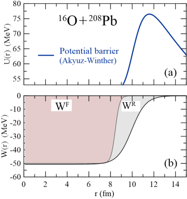
Figure 1: (Color on line) Panel (a): The Coulomb barrier for the São Paulo potential Chamon et al. (1997, 2002) in ${}^{16}{\rm O}\,-\,^{208}{\rm Pb}$ scattering; Panel (b): Imaginary potentials simulating pure fusion absorption ($W^{\rm\scriptscriptstyle F}$) and absorption arising from fusion and from direct reactions ($W^{\rm\scriptscriptstyle R}$). For detail, see the text.

An illustration of the imaginary potentials in the cases of pure fusion absorption ($W^{\rm\scriptscriptstyle F}$) and fusion plus direct reaction absorption ($W^{\rm\scriptscriptstyle R}$) for the ${}^{16}{\rm O}\,-\,^{208}{\rm Pb}$ scattering is presented in Fig. 1. In this example, the real part of the interaction is given by the Akyüz-Winther potential Broglia and Winther (2004); Akyüz and Winther (1981). Panel (a) shows the Coulomb barrier for this potential, whereas panel (b) shows the imaginary potentials $W^{\rm\scriptscriptstyle F}$ and $W^{\rm\scriptscriptstyle R}$. The potential $W^{\rm\scriptscriptstyle F}$ was evaluated by Eq. (3), with $W_{0}=50$ MeV, $r_{\rm 0i}=1.0$ fm and $a_{\rm 0i}=0.2$ fm, and $W^{\rm\scriptscriptstyle R}$ was obtained by multiplying the real part of the potential by the factor 0.78.

2.1 Fusion and total reaction cross sections

In potential scattering the absorption cross section is given by the partial-wave series

$$\sigma_{\rm abs}(E)=\frac{\pi}{k^{2}}\sum_{l=0}^{\infty}\,(2l+1)\,P_{\rm abs}\left(l,E\right),$$ (4)

where

$$P_{\rm abs}\left(l,E\right)=1-\left|S_{l}(E)\right|^{2}$$ (5)

is the absorption probability at the $l^{\rm\scriptscriptstyle th}$-partial wave, which is given by the deviation of the partial-wave component of the S-matrix, $S_{l}(E)$, from the unitary behaviour.

The absorption cross section can also be given in terms of the expectation value of the imaginary potential, through the expression

$$\sigma_{\rm abs}(E)=-\ \frac{1}{|A|^{2}}\ \frac{k}{E}\ \left\langle\psi^{\rm\scriptscriptstyle(+)}\left|\,W(r)\,\right|\,\psi^{\rm\scriptscriptstyle(+)}\right\rangle,$$ (6)

where $A$ is the normalization constant of the scattering wave function, $\psi^{\rm\scriptscriptstyle(+)}({\bf r})$. Eq. (6), can be easily derived from the continuity equation for the Schrödinger equation with the complex potential Canto and Hussein (2013). Carrying out the partial-wave expansion of Eq. (6), the reaction cross section takes the form of Eq. (4), with the absorption probabilities of Eq. (5) given by the radial integral

$$P_{\rm abs}\left(l,E\right)=-\frac{4k}{E}\int_{0}^{\infty}dr\ W(r)\,|u_{l}(k,r)|^{2},$$ (7)

with $u_{l}(k,r)$ standing for the radial wave function of the $l^{\rm th}$ partial wave, in a collision with wave number $k=\sqrt{2\mu E}/\hbar$, where $\mu$ stands for the reduced mass.

The relation between $\sigma_{\rm abs}(E)$ and the observable cross sections depends on the nature of the imaginary potential. When it simulates the influence of fusion plus direct reactions ($W(r)=W^{\rm\scriptscriptstyle R}(r)$), $\sigma_{\rm abs}(E)$ corresponds to the total reaction cross section. On the other hand, if one is interested in the fusion cross section, one should use a strong imaginary potential with a short-range. However, this does not guarantee fusion. For CN formation, the projectile and the target must remain in close proximity for a long time, long enough for the full thermalization of the excitation energy. This happens when the system is caught inside a pocked of the effective potential,

$$V_{l}(r)=V(r)\,+\,\frac{\hbar^{2}}{2\mu\,r^{2}}\ l(l+1),$$ (8)

which appears in the radial equation. Thus, the fusion cross section should be written,

$$\sigma_{\rm\scriptscriptstyle F}(E)=\frac{\pi}{k^{2}}\sum_{l=0}^{\infty}\,(2l+1)\,P_{\rm\scriptscriptstyle F}\left(l,E\right),$$ (9)

with

$$P_{\rm\scriptscriptstyle F}\left(l,E\right)=P_{\rm abs}\left(l,E\right)\times P_{\rm\scriptscriptstyle CN}\left(l,E\right).$$ (10)

Above, $P_{\rm\scriptscriptstyle CN}\left(l,E\right)$ is the probability of CN formation, after the system enters the strong absorption region. For low partial waves and near-barrier energies, this probability is very close to one. The situation is different for partial waves above the critical angular momentum, $l_{\rm cr}$. This angular momentum is defined as the highest $l$-value for which the potential $V_{l}(r)$ exhibits a pocket. Above $l_{\rm cr}$, $V_{l}(r)$ is strongly repulsive (dominated by the centrifugal term), decreasing monotonically with $r$. In this way, the system may enter the strong absorption region but it stays there for a short time, orders of magnitude shorter than that required for thermalization and CN formation. In this situation, the absorption corresponds to inelastic scattering, transfer or pre-equilibrium reactions, but definitely not to fusion. Therefore, partial-wave above $l_{\rm cr}$ should not be included in the calculation of fusion. This is is achieved by setting,

$$\mathcal{P}_{\rm\scriptscriptstyle CN}(l,E) = 1,\ \ \ {\rm for}\ l<l_{\rm cr}$$ (11)

$$= 0,\ \ \ {\rm for}\ \geq l_{\rm cr}.$$

There is an alternative to the use of a complex potential in the calculation of fusion cross sections. One can keep the potential real and adopt ingoing wave boundary conditions (IWBC) Feshbach et al. (1947); Rawitscher (1964, 1966); Canto et al. (2006) for the radial wave functions at the bottom of the pocked of $V_{l}(r)$, $R_{\rm in}$. The wave functions and their derivatives at $r=R_{\rm in}$ are then evaluated within the WKB approximation, and the radial equations are numerically integrated, from $R_{\rm in}$ to the matching radius. In an optical model calculation with a strong and short range imaginary potential, the incident waves reaching the inner region of the barrier are completely absorbed, so that there is no reflected wave coming out. In this way, radial wave functions obtained with $W^{\rm\scriptscriptstyle F}(r)$ are expected to be equivalent to those of a real potential with IWBC, and the same happens with the corresponding components of the S-matrix, $S_{l}(E)$.

The WKB approximation and the Hill-Wheeler transmission coefficient

The absorption probability in Eq. (5), $P_{\rm abs}(l,E)$, acquires a simple form in the WKB (Wentzel, Kramers, and Brillouin) approximation, where the radial wave functions are written in terms of the local wave numbers, $k_{l}(r)$, defined as,

$$\kappa_{l}(r)=\frac{1}{\hbar}\ \sqrt{V_{l}(r)+i\,W(r)-E}.$$ (12)

However, the explicit presence of the imaginary potential in $k_{l}(r)$ leads to extra difficulties in the calculation, as one has to deal with complex turning points (this will become clear in Eqs. (14) and (15)). Although, in principle, such calculation can be performed by resorting to the method of complex angular momenta (through the requirement that the imaginary part of the turning point is identically zero), practical usage of the results is limited.

The situation is better in calculations of fusion cross sections, where the imaginary potential is very strong but has a short-range. In this case, it absorbs completely the current that reaches the inner region of the barrier, but it is negligible elsewhere. It is still simpler in IWBC calculations, which are based on real potentials. In this case, the absorption probability at the partial-wave $l\,(\leq l_{\rm cr})$ is equal to the transmission coefficient of the incident wave through the barrier of $V_{l}(r)$, $T(l,E)$, namely

$$P_{\rm abs}(l,E)=P_{\rm\scriptscriptstyle F}\left(l,E\right)\simeq T(l,E).$$ (13)

Within Kemble’s improved version Kemble (1935) of the WKB approximation, the transmission coefficient is given by the expression

$$T(l,E)\simeq T^{\rm\scriptscriptstyle WKB}(l,E)=\frac{1}{1+\exp[2\,\Phi_{l}^{\rm\scriptscriptstyle WKB}(E)]},$$ (14)

where $\Phi_{l}^{\rm\scriptscriptstyle WKB}(E)$ is the integral of the local wave number evaluated along the classically forbidden region,

$$\Phi^{\rm\scriptscriptstyle WKB}_{l}(E)=\int_{r_{i}}^{r_{e}}\,\kappa_{l}(r)\ dr,$$ (15)

with $r_{i}$ and $r_{e}$ standing respectively for the internal and external classical turning points for the potential $V_{l}(r)$. These turning points are real at sub-barrier energies but they become complex above the barrier. Kemble argued that this problem could be solved through an analytical continuation of the radial variable to the complex plane. He pointed out that in the case of a parabolic barrier, discussed in the next sub-section, the integral of Eq. (15) is given by an analytical expression and this expression is valid for any collision energy, below or above the barrier. Recently, the analytical continuation of the radial variable for typical heavy-ion potentials was discussed, and the applicability of the Wong formula (see section 2.1) was extended to above-barrier energies Toubiana et al. (2017a, b).

Hill and Wheeler studied the transmission through the parabolic barrier

$$V(r)=V_{\rm\scriptscriptstyle B}-\frac{1}{2}\,\mu\omega^{2}\ \left(r-R_{\rm\scriptscriptstyle B}\right)^{2}.$$ (16)

In this case, the transmission coefficient can be evaluated exactly. The result, known as the Hill-Wheeler transmission factor, is

$$T(E)=\frac{1}{1+\exp\left[2\pi\,\left(V_{\rm\scriptscriptstyle B}-E\right)/\hbar\omega\right]}.$$ (17)

Approximate expression for heavy-ion fusion cross sections can be obtained by taking the Hill-Wheeler transmission function to obtain the fusion probabilities. For this purpose, the effective $l$-dependent potentials are approximated by a parabola, as

$$V_{l}(r)=B_{l}-\frac{1}{2}\,\mu\omega_{l}^{2}\ \left(r-R_{l}\right)^{2},$$ (18)

where $B_{l}$, $R_{l}$ and $\hbar\omega_{l}$ are respectively the height, radius and curvature parameter of the barrier for the $l^{\rm th}$-partial wave. The corresponding transmission coefficients are, then, given by the expression,

$$T^{\rm\scriptscriptstyle HW}(l,E)=\frac{1}{1+\exp\left[2\pi\,\left(B_{l}-E\right)/\hbar\omega_{l}\right]}.$$ (19)

If the imaginary potential has a short range, as the case of $W^{\rm\scriptscriptstyle F}(r)$ in Fig. 1, absorption is equivalent to fusion and the fusion probabilities should be very close to the corresponding transmission coefficients. However, this assumption is meaningless for partial-waves above $l_{\rm cr}$, where the potential $V_{l}(r)$ decreases monotonically as $r$ increases. To deal with this problem, one truncates the partial-wave series for $\sigma_{\rm\scriptscriptstyle F}$ at $l=l_{\rm cr}$. In this way, the WKB approximation for $\sigma_{\rm\scriptscriptstyle F}$ contains the implicit assumption that the factor $P_{\rm\scriptscriptstyle CN}(l,E)$ of Eq. (10) is equal to one below $l_{\rm cr}$ and zero otherwise. The fusion cross section in the WKB approximation can be written,

$$\sigma_{\rm\scriptscriptstyle F}(E)=\frac{\pi}{k^{2}}\sum_{l=0}^{l_{\rm cr}}(2l+1)\ T^{\rm\scriptscriptstyle HW}(l,E).$$ (20)

The quality of the parabolic approximation for the potential barriers depends on the collision energy and on the mass of the system. It is reasonable at near-barrier energies but becomes very inaccurate at energies well below the Coulomb barrier. It works fairly well for heavy systems even at collision energies several MeV below the Coulomb barrier. However, this approximation is quite poor for light heavy ions Canto et al. (2006). A common practice that leads to a very accurate fusion cross section is to use Kemble’s transmission coefficients (Eq. (14)) below the Coulomb barrier and the Hill-Wheeler transmission factors (Eq. (19)) above.

Poisson series and the Wong formula

The sum of partial waves giving the fusion cross section can be transformed into a rapidly converging series of integrals. According to the Poisson formula, we can write

$$\sigma_{\rm\scriptscriptstyle F}(E)=\frac{\pi}{k^{2}}\ \sum_{l=0}^{\infty}(2l+1)\,T(l,E)\\ =\frac{2\pi}{k^{2}}\sum_{m=0,\pm 1,...}(-)^{m}\int\lambda\ T\left(\lambda,E\right)e^{2i\pi m\,\lambda}\ d\lambda,$$ (21)

where

$$\lambda=l+1/2\ \ \ {\rm and}\ \ \ T_{l}(E)=T\left(\lambda,E\right).$$

The sum over $m$ converges very rapidly, so that, in most cases, it is enough to consider the leading term, with $m=0$.

Wong Wong (1973) obtained a very useful expression for the fusion cross section by considering only the $m=0$ term of the Poisson series and making additional approximations on the $l$-dependent effective potential. First, he adopted the parabolic approximations of Eq. (18). Next, he neglected the $l$-dependences of the $R_{l}$ and $\hbar\omega_{l}$ and made the approximations,

$$R_{l} = R_{l=0}\equiv R_{\rm\scriptscriptstyle B}$$

$$\hbar\omega_{l} = \hbar\omega_{l=0}\equiv\hbar\omega,$$

$$B_{\rm\scriptscriptstyle\lambda} \simeq V_{\rm\scriptscriptstyle B}+\frac{\hbar^{2}\lambda^{2}}{2\mu\,R_{\rm\scriptscriptstyle B}^{2}}.$$ (22)

With these approximations the integral over $\lambda$ can be carried out analytically and one gets the so-called Wong cross section Wong (1973)

$$\sigma^{\rm\scriptscriptstyle W}(E)=\frac{\hbar\omega\,R_{\rm\scriptscriptstyle B}^{2}}{2E}\ \ln{\left[1+\exp{\left(\frac{2\pi}{\hbar\omega}(E-V_{\rm\scriptscriptstyle B})\right)}\right]}.$$ (23)

At low enough sub-barrier energies ($E\ll V_{\rm\scriptscriptstyle B}-\hbar\omega$), Eq. (23) may be approximated by the simpler expression,

$$\sigma_{\rm\scriptscriptstyle F}(E)\simeq\frac{\hbar\omega\,R_{\rm\scriptscriptstyle B}^{2}}{2E}\ \exp\left[-2\pi\,\frac{\left|E-V_{\rm\scriptscriptstyle B}\right|}{\hbar\omega}\right].$$ (24)

A simpler approximation for the Wong formula can also be derived at energies few MeV above the Coulomb barrier $(E\gtrsim V_{\rm\scriptscriptstyle B}+\hbar\omega$). In this energy region one can neglect the unity within the square bracket of Eq. (23), and it becomes

$$\sigma_{\rm\scriptscriptstyle F}(E)\simeq\sigma_{\rm geo}\ \left[1-\frac{V_{\rm\scriptscriptstyle B}}{E}\right],$$ (25)

where

$$\sigma_{\rm geo}=\pi\ R_{\rm\scriptscriptstyle B}^{2}$$ (26)

is the geometric cross section.

Wong’s formula is quite accurate in collisions of heavy systems at near-barrier energies (say $V_{\rm\scriptscriptstyle B}+5\,{\rm MeV}\geq E\geq V_{\rm\scriptscriptstyle B}-5\,{\rm MeV}$). However, it is a poor approximation in collisions of light systems, both below and above the Coulomb barrier. The problem at sub-barrier energies is that the barrier for light systems is highly asymmetric, whereas the parabolic approximation is symmetric. The tail of $V(r)$ falls off slowly, as the Coulomb potential ($\sim 1/r$), while the parabola goes to zero much faster. Thus, the external turning points for the two potentials become very different as the energy decreases, with $r_{\rm e}$ for the parabola being progressively smaller. In this way, the function $\Phi^{\rm\scriptscriptstyle WKB}_{l}(E)$ for the parabola is too small, and the transmission coefficient of Eq. (14) is badly overestimated. For example, the fusion cross section for the ${}^{6}{\rm Li}\,+\,^{12}{\rm C}$ system predicted by the Wong formula at $E=1$ MeV ($V_{\rm\scriptscriptstyle B}\simeq 3$ MeV) is more than two orders of magnitude larger than the value obtained by a quantum mechanical calculations (see Fig. 26 of Ref. Canto et al. (2006)). The inaccuracy of the Wong formula above the Coulomb barrier has another origin. Contrary to what was assumed in the derivation of the Wong formula, the parameters $R_{l}$ and $\omega_{l}$ for light systems have a strong $l$-dependence.

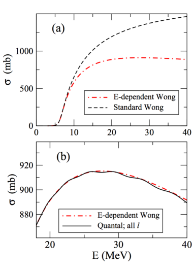
Figure 2: (Color on line) Fusion cross sections for the ¹²C + ¹²C system. Panel (a): Comparison of the energy-dependent Wong formula (red dot-dashed curve) with the standard Wong formula (dashed curve); Panel (b): Comparison of the energy-dependent Wong formula with the exact cross section, calculated by full quantum mechanics (solid line). The figure was taken from Ref. Rowley and Hagino (2015).

Rowley and Hagino Rowley and Hagino (2015) have shown that the accuracy of the Wong formula for light systems at above-barrier energies is significantly improved if one replaces the s-wave barrier parameters in Eq. (23) by the barrier parameters associated with the grazing angular momentum, $R_{\scriptscriptstyle E}$, $\hbar\omega_{\scriptscriptstyle E}$ and $V_{\scriptscriptstyle E}$. This is illustrated in Fig. 2. Panel (a) shows a comparison of the standard Wong cross section with the one obtained using the parameters associated with the grazing angular momentum at the corresponding collision energy, $E$. One observes that the two cross sections become progressively different as the energy increases. At 40 MeV, the standard Wong cross section is about 3/2 of the one obtained with the energy dependent parameters.

Panel (b) shows a comparison of the energy-dependent Wong formula with exact results of full quantum mechanics. One concludes that the improved Wong formula of Ref. Rowley and Hagino (2015) is a very good approximation to the quantum mechanical cross section.

Usually, higher order terms of the Poisson series give negligible contributions to the fusion cross section. The situation is slightly different in the case of identical nuclei. These contributions are responsible for the weak oscillations in the exact fusion cross section of the ¹²C + ¹²C system (solid line on panel (b) of Fig. 2). Adding these contributions to the energy-dependent Wong formula, Rowley and Hagino were able to reproduce the quantum mechanical cross section of Fig. 2 with great accuracy Rowley and Hagino (2015). Recently, the study of Rowley and Hagino has been extended to collisions of identical nuclei with arbitrary spin Toubiana et al. (2017c).

The Wong formula at $E>E_{\rm cr}$

Eq. (25) indicates that the cross section tends to a constant value as the energy goes to infinity, This is not consistent with the prediction of quantum mechanics in potential scattering, where the cross section goes to zero in the $E\rightarrow\infty$ limit. The origin of this discrepancy is that Wong assumes that the radii and the shapes of the barriers of the effective potentials are independent of $l$. In this way the partial-wave series always gets important contributions from waves around the grazing angular momentum, given by the condition $V_{l_{\rm g}}(R_{l})=E$. The situation is quite different for the actual potential. In the WKB calculation, the fusion probability vanishes above $l_{\rm cr}$, since $V_{l}(r)$ has no barrier. On the other hand, in the quantum mechanical calculation, the partial-wave series of Eq. (9) is limited by the factor $P_{\rm\scriptscriptstyle CN}(l,E)$, that vanishes above $l_{\rm cr}$. Owing to the repulsive nature of the potential, the collision time is not long enough to allow the formation of an equilibrated CN. Thus, both in quantum mechanical calculation and in the WKB approximation with the actual effective potential, the partial-wave series is truncated at $l=l_{\rm cr}$. At high enough energies, all non-vanishing fusion probabilities are equal to one and the partial-wave series can be summed analytically. This establishes a new energy regime, where the fusion cross section decreases monotonically with $E$, according to the expression,

$$\sigma_{\rm\scriptscriptstyle F}\left(E\right)\simeq\sigma_{0}\times\frac{E_{\rm cr}}{E},$$ (27)

with

$$\sigma_{0}=\frac{\pi\hbar^{2}\left(l_{\rm cr}+1\right)^{2}}{2\mu E_{\rm\scriptscriptstyle cr}}.$$ (28)

Wong formula vs. $\sigma_{\rm\scriptscriptstyle R}$

The derivation of the Wong formula is based on the assumption that the absorption probability is equal to the transmission coefficient through the barrier of the real potential of Eq. (8). This assumption is consistent with the IWBC or calculations with a very strong imaginary potential acting exclusively in the inner region of the barrier. Thus, Wong’s formula is an approximation for the fusion cross section. It is expected to be a poor approximation for the total reaction cross section, since it may get important contributions from direct reactions, which correspond to absorption in the barrier region and beyond. Nevertheless, in Wong’s original paper Wong (1973) and in other publications it has been taken as an approximation for $\sigma_{\rm\scriptscriptstyle R}$. In such cases, $R_{\rm\scriptscriptstyle B}$, $V_{\rm\scriptscriptstyle B}$ and $\hbar\omega$ should be interpreted as effective quantities, rather than the parameters extracted from the parabolic fit of the real potential.

2.2 The semiclassical scattering amplitude

The partial-wave expansion of the nuclear part of the scattering amplitude is given by Canto and Hussein (2013)

$$f_{\rm\scriptscriptstyle N}(\theta)=\frac{1}{2ik}\,\sum_{l=0}^{\infty}(2l+1)\,P_{l}(\cos\theta)\ e^{2i\sigma_{l}}\Big{[}\left|S_{\rm\scriptscriptstyle N}(l,E)\right|\,e^{2i\delta_{l}}-1\Big{]},$$ (29)

where $\sigma_{l}$ and $\delta_{l}$ are respectively the Coulomb and the nuclear phase-shifts at the $l^{\rm th}$ partial-wave, $\left|S_{\rm\scriptscriptstyle N}(l,E)\right|$ is the modulus of the nuclear S-matrix and $P_{l}(\cos\theta)$ is the Legendre polynomial. The semiclassical scattering amplitude is obtained through the following approximations.

1. use the Poisson series to evaluate the partial-wave sum;

2. evaluate nuclear phase-shifts within the WKB approximation;

3. use Legendre polynomials of continuous order ($\lambda$) and adopt the large $\lambda$ approximation:

   $$P_{l}(\cos\theta)\ \ \longrightarrow\ \ P(\lambda,\cos{\theta})\simeq\left(\frac{1}{2\pi\lambda\sin{\theta}}\right)^{1/2}\\ \left[e^{i\left(\lambda\theta-\pi/4\right)}+e^{-i\left(\lambda\theta-\pi/4\right)}\right];$$ (30)

4. evaluate integrals using the stationary phase approximation.

With the above approximations, one can infer several characteristic features of heavy-ion scattering. The two terms within square brackets in Eq. (30) give rise to a near and a far component of the scattering amplitude and to near-far and rainbow oscillations of the cross section in heavy-ion elastic scattering.

The Fresnel diffraction formula and the quarter point recipe

Heavy-ion scattering is dominated by Coulomb repulsion and strong absorption. This leads to the sharp cut-off model (black disk approximation) for charged particle scattering at low energies. In this model, nuclear phase shifts are neglected and the $l$-projected components of the S-matrix are given by,

$$S(l)\equiv\left|S_{\rm\scriptscriptstyle N}(l,E)\right|\,e^{2i(\sigma_{l}+\delta_{l})}\rightarrow S(\lambda)\simeq{\mathcal{H}}\left(\lambda-\bar{\Lambda}\right)\ e^{2i\sigma(\lambda)}.$$ (31)

Above, $\bar{\Lambda}$  is the grazing angular momentum and

$${\mathcal{H}}\left(\lambda-\bar{\Lambda}\right) = 1,\ {\rm for}\ \lambda\geq\bar{\Lambda}$$ (32)

$$= 0,\ {\rm for}\ \lambda<\bar{\Lambda}$$ (33)

is the Heaviside step function.

Within the sharp cut-off model of the semiclassical scattering amplitude, the elastic cross section is dominated by the interference between a refractive Coulomb wave at $\lambda>\bar{\Lambda}$ and a diffractive wave for smaller values of $\lambda$. Frahn Frahn (1966, 1985) demonstrated that the ratio of the elastic scattering cross section with respect to the corresponding Rutherford cross section, which will be denoted by $\sigma(\theta)/\sigma_{\rm\scriptscriptstyle C}(\theta)$, is given by the Fresnel diffraction formula

$$\frac{\sigma(\theta)}{\sigma_{\rm\scriptscriptstyle C}(\theta)}=\frac{1}{2}\left[\left(\frac{1}{2}-C({\scriptstyle W})\right)^{2}+\left(\frac{1}{2}-S({\scriptstyle W})\right)^{2}\right],$$ (34)

where $C({\scriptstyle W})$ and $S({\scriptstyle W})$ are the Fresnel integrals given by,

$$C({\scriptstyle W})=\int_{0}^{\scriptstyle W}d\omega\cos{\left(\frac{\pi}{2}\omega^{2}\right)}$$ (35)

and

$$S({\scriptstyle W})=\int_{0}^{\scriptstyle W}d\omega\sin{\left(\frac{\pi}{2}\omega^{2}\right)}.$$ (36)

The argument of the Fresnel integrals is

$${\scriptstyle W}=\sqrt{\frac{2\eta}{\pi}}\ \left[\frac{\sin\left(\frac{\theta-\bar{\Theta}}{2}\right)}{\sin{\frac{\bar{\Theta}}{2}}}\right],$$ (37)

where $\eta$ is the Sommerfeld parameter, $\theta$ is the scattering angle and $\bar{\Theta}$ is the grazing angle.

An important property of the Fresnel integrals is that they vanish at ${\scriptstyle W}=0$ (this can be immediately checked in Eqs. (35) and (36)). This value of ${\scriptstyle W}$ is reached at the scattering angle $\theta=\bar{\Theta}$. Using these results in Eq. (34), the ratio of the cross sections at the grazing angle becomes

$$\frac{\sigma(\bar{\Theta})}{\sigma_{\rm\scriptscriptstyle C}(\bar{\Theta})}=\frac{1}{4}.$$ (38)

To emphasize this property, the grazing angle is denoted

$$\bar{\Theta}=\theta_{\rm\scriptscriptstyle 1/4}.$$

Figure 3: Fresnel diffraction within the sharp cut-off approximation. Figure from Ref. Canto and Hussein (2013).

An important consequence of Eq. (38) is that the grazing angle can be determined directly from the scattering data: $\bar{\Theta}$ is the angle where $\sigma(\theta)/\sigma{\rm\scriptscriptstyle C}(\theta)$ reaches the value 1/4. Having $\bar{\Theta}$, one can determine the argument ${\rm\scriptscriptstyle W}$ for each value of $\theta$, and evaluate the Fresnel integrals. Then, inserting them into Eq. (34), one obtains $\sigma(\theta)/\sigma_{\rm\scriptscriptstyle C}(\theta)$, within the sharp cut-off approximation for the S-matrix. This result is known as Frahn’s Fresnel diffraction formula for the angular distribution.

An illustration of this procedure is given in Fig. 3, for the ¹⁶O + ²⁰⁸Pb collision. This example was discussed in detail by Frahn Frahn (1966). In this case, the grazing angle is $\theta_{\rm\scriptscriptstyle 1/4}=40.9^{\rm o}$, ${\bar{\Lambda}}=86$ and the Sommerfeld parameter is $\eta=32.05$. Frahn Frahn (1966) has shown that the predictions of the sharp cut-off model are in qualitative agreement with the data. It predicts oscillations at low scattering angles (illuminated region) with increasing amplitudes, which ends in a pronounced maximum, followed by a rapid decrease of $\sigma(\theta)/\sigma_{\rm\scriptscriptstyle C}(\theta)$ as $\theta$ increases (shadow region). However, the Fresnel diffraction formula completely ignores the effects of nuclear refraction. These effects are responsible for other kind of oscillations, like near-far interference and the rainbow. One should stress that rainbow scattering with a unitary S-matrix leads also to the typical pattern of heavy-ion scattering, exhibited in Fig. 3. Quantum mechanical potential scattering calculations with complex potentials, which include both refractive and diffractive effects of the nuclear potential, lead to more quantitative prediction of the elastic angular distributions.

The sharp cut-off model can also be used to make qualitative prediction of total reaction cross sections. From the experimental $\sigma(\theta)/\sigma_{\rm\scriptscriptstyle C}(\theta)$ ratio at a given collision energy, $E$, one determines the grazing angle. Then, one finds the grazing angular momentum from the Rutherford trajectory by the equation,

$$\bar{\Lambda}(E)=\eta\ \cot\left(\frac{\theta_{\rm\scriptscriptstyle 1/4}}{2}\right).$$ (39)

Next, we evaluate the total reaction cross section taking Eq. (4) and replacing the partial-wave sum by an integral over $\lambda$. This corresponds to taking only the $m=0$ term in the Poisson series (see e.g. Ref. Canto and Hussein (2013)). One gets

$$\sigma_{\rm\scriptscriptstyle R}(E)=\frac{2\pi}{k^{2}}\int d\lambda\,\lambda\ P(\lambda,E).$$ (40)

Using the sharp cut-off model, the absorption (reaction) probability of Eq. (5) becomes

$$P_{\rm abs}(\lambda,E)=1-{\mathcal{H}}(\lambda-\bar{\Lambda}{\rm\scriptscriptstyle(E)})={\mathcal{H}}(\bar{\Lambda}{\rm\scriptscriptstyle(E)}-\lambda).$$ (41)

Then, the integral of Eq. (40) can be immediately evaluated and one gets

$$\sigma_{\rm\scriptscriptstyle R}=\frac{\pi}{k^{2}}\ \bar{\Lambda}^{2}(E).$$ (42)

It is worth mentioning that at higher energies, the Coulomb effect becomes small and the angular distribution corresponding to the black disk or sharp cutoff model approximates the Fraunhoffer diffraction. The grazing angular momentum can still be obtained from the angular period of oscillations, $\Delta\theta=\pi/\bar{\Lambda}$.

2.3 The Generalized Optical Theorem and the Sum of Differences Method

The Optical Theorem is an important result in scattering theory and it expresses unitarity in a useful mathematical form. For uncharged particle scattering, the theorem states that the total (angle integrated) elastic scattering cross section is proportional to the imaginary part of the elastic amplitude evaluated at $\theta=0$. In potential scattering from a real potential, one has

$$\int\ \frac{d\sigma_{\rm el}(\theta)}{d\Omega}\ d\Omega=\frac{4\pi}{k}\ {\rm Im}\left\{f_{\rm el}(\theta=0)\right\}.$$ (43)

When absorption is present, the above becomes the Generalized Optical Theorem (GOT),

$$\int\ \frac{d\sigma_{\rm el}(\theta)}{d\Omega}\ d\Omega+\sigma_{\rm\scriptscriptstyle R}=\frac{4\pi}{k}{\rm Im}\left\{f_{\rm el}(\theta=0)\right\}.$$ (44)

For charged particles, the GOT needs to be modified to cope with the point Coulomb singularity. The integral in Eqs. (43) and (44) is divergent. First, the scattering amplitude is written as

$$f_{\rm el}(\theta)=f_{\rm\scriptscriptstyle C}(\theta)\,+\,f_{\rm\scriptscriptstyle N}(\theta),$$ (45)

where $f_{\rm\scriptscriptstyle C}(\theta)$ is the Coulomb scattering amplitude for two point charges, and $f_{\rm\scriptscriptstyle N}(\theta)$ is a correction arising from the short-range nuclear potential. The former is given by the analytical expression,

$$f_{\rm\scriptscriptstyle C}(\theta) = \frac{\eta}{2k\sin^{2}{(\theta/2})}\ e^{i\,\left[2\sigma_{0}+\pi-2\eta\,\ln\left(\sin\theta/2\right)\right]}$$ (46)

$$= -\frac{\eta}{k}\ 2^{i\eta}\ \frac{e^{2i\sigma_{0}}}{(1-\cos{\theta})^{i\eta+1}}\ ,$$

and the latter is given by the partial-wave expansion,

$$f_{\rm\scriptscriptstyle N}(\theta)=\frac{1}{2ik}\ \sum_{l=0}^{\infty}(2l+1)\ e^{2i\sigma_{l}}\ \big{[}S_{\rm\scriptscriptstyle N}(l)-1\big{]}\ P_{l}(\cos{\theta}).$$ (47)

To get rid of the singularity, the GOT for charged particles is expressed in terms of the difference

$$\sigma_{\rm\scriptscriptstyle SOD}\left(\theta_{0}\right)=\ 2\pi\ \int_{\theta_{0}}^{\pi}\ \left[\frac{d\sigma_{\rm\scriptscriptstyle Ruth}(\theta)}{d\Omega}\ -\ \frac{d\sigma_{\rm\scriptscriptstyle el}(\theta)}{d\Omega}\right]\,\sin\theta\,d\theta,$$ (48)

where $\theta_{0}$ is a very small angle. The cross section difference, $\sigma_{\rm\scriptscriptstyle SOD}\left(\theta_{0}\right)$, is called the sum-of-difference (SOD) cross section. The replacement $\theta=0\rightarrow\theta=\theta_{0}$ in the lower limit of the integration is justified by the fact that, in a realistic collision, the Coulomb potential is screened.

Using the explicit forms of the elastic and the Coulomb cross sections, namely

$$\frac{d\sigma_{\rm el}(\theta)}{d\Omega}=\big{|}f_{\rm\scriptscriptstyle C}(\theta)\,+\,f_{\rm\scriptscriptstyle N}(\theta)\big{|}^{2};\ \ \ \frac{d\sigma_{\rm\scriptscriptstyle C}(\theta)}{d\Omega}=\big{|}f_{\rm\scriptscriptstyle C}(\theta)\big{|}^{2},$$ (49)

Eq. (48) becomes

$$\sigma_{\rm\scriptscriptstyle SOD}\left(\theta_{0}\right)=-\ 2\pi\,\int_{\theta_{0}}^{\pi}\left|f_{\rm\scriptscriptstyle N}(\theta)\right|^{2}\,\sin\theta\ d\theta\\ -\,4\pi\,\int_{\theta_{0}}^{\pi}{\rm Re}\left\{f_{\rm\scriptscriptstyle C}^{*}(\theta)\cdot f_{\rm\scriptscriptstyle N}(\theta)\right\}\,\sin\theta\ d\theta.$$ (50)

The above cross section has been discussed by several author Holdeman and Thaler (1965a, b); Marty (1983); Ueda et al. (1999); Barrette and Alamanos (1985a, b); Ostrowski et al. (1991a). Marty evaluated the integrals of Eq. (50) and obtained the SOD cross section,

$$\sigma_{\rm\scriptscriptstyle SOD}(\theta_{0})\,=\,\sigma_{\rm\scriptscriptstyle R}-\frac{4\pi}{k}\ \left|f_{\rm\scriptscriptstyle N}(0)\right|\,\\ \times\sin{\Big{[}\arg\left\{f_{\rm\scriptscriptstyle N}(0)\right\}\,-\,2\sigma_{0}+\eta\ln\left\{\sin^{2}{\theta_{0}/2}\right\}\Big{]}}\ +\ O\left(\theta_{\rm\scriptscriptstyle 0}^{\rm\scriptscriptstyle 2}\right).$$ (51)

Above, $\eta$ is the Sommerfeld parameter, $\sigma_{0}$ is the s-wave Coulomb phase shift, and $O\left(\theta_{0}^{2}\right)$ is a correction, that becomes negligible when $\theta_{0}$ is a very forward angle.

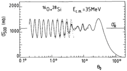
Figure 4: The SOD cross section for the ${}^{16}{\rm O}\,+\,^{28}{\rm Si}$ system at $E_{\rm c.m.}=35$ MeV. The solid line and the dashed lines correspond respectively to the exact result of Eq. (48), and the approximation of Eq. (51). The calculations adopted the optical potential of Shkolnik et al. Shkolnik et al. (1978) (figure taken from Ref. Barrette and Alamanos (1985a)).

The accuracy of Eq. (51) is illustrated in Fig. 4, where the approximate cross section of Eq. (51) and the exact result of Eq. (48) are compared. In this example, taken from Ref. Barrette and Alamanos (1985a), $\sigma_{\rm\scriptscriptstyle el}(\theta)$ and $f_{\rm\scriptscriptstyle N}(0)$ were calculated with the optical potential of Ref. Shkolnik et al. (1978). Clearly, the approximation is quite accurate for small values of $\theta_{0}$. The oscillatory behaviour of $\sigma_{\rm\scriptscriptstyle SOD}(\theta_{0})$ at forward angles provide two important pieces of information. First, the total reaction cross section is given by the SOD cross section averaged over a period of oscillation in the low $\theta_{0}$ region. Thus, the total reaction cross section can be determined from accurate measurements of the elastic cross section at forward angles. The use of this technique is discussed in sect. 5.2.

The second important consequence of Eq. (51) is that the modulus of $f_{\rm\scriptscriptstyle N}(0)$ can be extracted from the period of oscillation. This equation has been fully analysed in the context of heavy-ions collisions Barrette and Alamanos (1985a, b); Ostrowski et al. (1991b); Ueda et al. (1998, 1999). In most of the applications of Eq.(51), the aim was to study the oscillations in the nuclear amplitude at forward angles, which can be traced to forward glory effects. The existence of a non-zero value of the impact parameter, $b_{\rm gl}$, at which the classical deflection angle defined through the relation,

$$\Theta(l)=2\,\frac{\delta(\sigma_{l}+\delta_{l})}{\delta l}.$$

satisfies the condition $\Theta(b_{\rm gl})=0$, corresponds to forward glory. Under this condition, the scattering amplitude at forward angles is enhanced and with conspicuous oscillations. In fact, this nuclear amplitude, $f_{\rm\scriptscriptstyle N}(\theta)$, in the vicinity of the forward glory angle ($\theta=0^{o}$) is given by the product $A(\theta)J_{0}(\lambda_{\rm gl}\theta)$, where $J_{0}$ is the Bessel function of order zero and $A(\theta)$ is a smooth function of $\theta$. Thus the SOD method, in the presence of forward glory, would supply a reaction cross section with greatly enhanced energy oscillations Barrette and Alamanos (1985a, b); Ueda et al. (1999). Besides this, the forward glory effect can be used to learn more about the nuclear interaction at the surface region, complementary to the information obtained from the study of nuclear rainbow scattering, as emphasised in Ref. Ueda et al. (1999).

2.4 Comparison of Quantum mechanical cross sections with the Wong and the quarter-point approximations

In potential scattering, fusion and direct reactions are taken into account through the inclusion of an imaginary part in the nucleus-nucleus potential. This procedure leads to reasonable predictions for $\sigma_{\rm\scriptscriptstyle F}$ and $\sigma_{\rm\scriptscriptstyle R}$. These cross sections are calculated by Eq. (4), with absorption probabilities expressed in terms of the unitarity defect of the S-matrix (Eq. (5)), or with the radial integrals involving the imaginary potential (Eq. (7)). However, calculations of fusion and of total reaction cross sections must use different imaginary potentials, as discussed in section 2. In the previous sections we discussed also the Wong formula and the quarter-point recipe, where the cross sections are approximated by simple analytical expressions. Now we discuss the validity of these approximations.

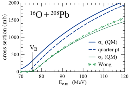
Figure 5: (Color on line) Quantum mechanical total reaction (thick blue solid line) and fusion (thin solid green line) cross sections, in comparison with the Wong cross section of Eq. (22) (green dot-dashed line with open circles) and the quarter point recipe cross section of Eq. (42) (blue dashed line).

As an example, let us consider the potential model for the ${}^{16}{\rm O}\,-\,^{208}{\rm Pb}$ collision, adopting the São Paulo Potential Chamon et al. (1997, 2002) for the real part of the nucleus-nucleus potential. In calculations of $\sigma_{\rm\scriptscriptstyle F}$, the imaginary potential is given by a short range WS function with the parameters: $W_{0}=50$ MeV, $r_{0i}=1.0$ fm and $a_{i}=0.2$ fm. In calculations of $\sigma_{\rm\scriptscriptstyle R}$, the imaginary part of the potential is proportional to its real part, $W(r)=0.78\ V(r)$. This prescription has been successfully used to describe the average behaviour of total reaction cross sections of many systems  Gasques et al. (2006). In Fig 5, the two quantum mechanical cross sections are shown in comparison with the ones obtained using the Wong formula and the quarter point recipe. The quarter point cross section (blue dashed line) was obtained by Eqs. (42) and (39), using in the latter the quarter point angle extracted from angular distributions of the quantum mechanical calculations, using $W^{\rm\scriptscriptstyle R}(r)$. Therefore, it is should be compared to $\sigma_{\rm\scriptscriptstyle R}$. We find that it underestimates the quantum mechanical cross section systematically. The difference between the two cross section is roughly constant, except at energies just above the barrier, where this approximation cannot be applied. In this region, $\theta_{\rm\scriptscriptstyle 1/4}$ is not defined, since the ratio between the elastic cross section and its Coulomb counterpart is above 1/4 for any scattering angle.

Now let us consider the Wong cross section. We note that it is very close to the fusion cross section, except at the higher energies ($E>100$ MeV). Although this approximation is known to become progressively poorer as the energy falls well below the Coulomb barrier Canto et al. (2006), this shortcoming cannot be observed in Fig. 5. However, it would be clear in a logarithmic scale plot. We should remark that it is not a surprise that the Wong cross section falls well below $\sigma_{\rm\scriptscriptstyle R}$. In the derivation of his formula, Wong approximates the absorption probability at each partial-wave by the transmission coefficient through the barrier of the $l$-dependent effective potential. This approximation implies that there is total absorption of the current that reaches the inner region of the barrier, but no absorption in the barrier region. This procedure is justified in the case of fusion absorption but it does not account for absorption arising from direct reactions, which gives an important contribution to $\sigma_{\rm\scriptscriptstyle R}$.

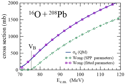
Figure 6: (Color on line) The quantum mechanical total reaction cross section (thick blue solid line) and Wong’s cross sections obtained with the barrier parameters of the são Paulo potential, and with barrier parameters fitted as to reproduce the quantum mechanical cross section. The notation is indicated in the legend of the figure.

To finish this sub-section, we point out that, in the original paper of Wong, his formula was presented as an approximation for the total reaction cross section. This may be reasonable if the reaction cross section is dominated by the fusion process. However, contributions of direct reactions can hardly be neglected. This becomes clear when one tries to compare reduced reaction cross section for different systems. Although the reduction method of Ref. Canto et al. (2009a, b), which is based on the Wong formula works fine for fusion data, it fails when applied to total reaction data Canto et al. (2015b). Nevertheless, the Wong formula can be a very good parameterization of the total reaction cross section, if $V_{\rm\scriptscriptstyle B},R_{\rm\scriptscriptstyle B}$ and $\hbar\omega$ are treated as adjustable parameters, fitted to the total reaction data. This is illustrated in Fig. 6, where the quantum mechanical cross section, $\sigma_{\rm\scriptscriptstyle R}$ (blue solid line), is compared with results of the Wong formula (green dot-dashed line with open circles) with the barrier parameters of the São Paulo potential, $R_{\rm\scriptscriptstyle B}=11.7$ fm, $V_{\rm\scriptscriptstyle B}=76.0$ MeV and $\hbar\omega=4.8$ MeV, and with the Wong formula with barrier parameters fitted to reproduce the quantum mechanical cross section (purple dotted line and open squares). The total reaction cross section given by the Wong formula with the parameters of the São Paulo potential falls well below its quantum mechanical counterpart. On the other hand, the cross section given by the Wong formula with the fitted parameters can hardly be distinguished from the quantum mechanical result. However, we stress that using barrier parameters which do not correspond to the actual potential has no physical meaning. In this case, the Wong formula is just a smart parameterization for the total reaction cross section.

3 Many-body scattering theory

Potential scattering is a very limited theory for heavy-ion collisions. In typical situations, the dynamics is strongly influenced by the nuclear structure of the collision partners, and then the coupled channel (CC) theory is a more suitable approach. In this treatment, the intrinsic degrees of freedom of the projectile and/or the target, denoted by $\xi$, are explicitly taken into account. The scattering wave function, ${\rm\Psi}^{\rm\scriptscriptstyle(+)}({\bf R},\xi)$, where ${\bf R}$ in the vector joining the centers of the collision partners, is the solution of the Schrödinger equation,

$$\big{[}E-\mathbb{H}\big{]}\,{\rm\Psi}^{\rm\scriptscriptstyle(+)}({\bf R},\xi)=0,$$ (52)

with scattering boundary conditions. Above,

$$\mathbb{H}=h(\xi)+\hat{K}+\mathbb{U}({\bf R},\xi)$$ (53)

is the total Hamiltonian of the system, $\hat{K}$ is the kinetic energy operator associated with the projectile-target relative motion, $h(\xi)$ is the intrinsic Hamiltonian, and $\mathbb{U}({\bf R},\xi)$ is the complex coupling interaction. In the CC method, the scattering wave function is expanded on a set of eigenstates of the intrinsic Hamiltonian (channels), $\varphi_{\alpha}(\xi)$, given by the eigenvalue equation,

$$h\,\varphi_{\alpha}(\xi)=\varepsilon_{\alpha}\ \varphi_{\alpha}(\xi),$$ (54)

where $\alpha$ stands for the set of quantum numbers required to specify the intrinsic state (usually the energy and the appropriate angular momentum quantum numbers, $lsj$ and $m$). That is

$${\rm\Psi}^{\rm\scriptscriptstyle(+)}({\bf R},\xi)=\sum_{\alpha=0}^{N}\varphi_{\alpha}(\xi)\,\psi_{\alpha}^{\rm\scriptscriptstyle(+)}({\bf R}).$$ (55)

Although the channel expansion involves an infinite number of intrinsic states, there is a finite number of nonelastic states, denoted by $N$, that are relevant to the reaction dynamics. Thus, the series is truncated after $N+1$ terms (the elastic, labelled by $\alpha=0$, and $N$ nonelastic channels).

3.1 The CC equations

Inserting the channel expansion into Eq. (52), taking scalar products with each of the intrinsic states, and using their orthonormality properties, one gets the set of CC equations

$$\big{[}E-H_{\alpha}({\bf R})\big{]}\,\psi_{\alpha}^{\rm\scriptscriptstyle(+)}({\bf R})=\sum_{\alpha^{\prime}}H_{\alpha,\alpha^{\prime}}({\bf R})\,\psi_{\alpha^{\prime}}^{\rm\scriptscriptstyle(+)}({\bf R}),$$ (56)

where $\alpha$ and $\alpha^{\prime}$ run from 0 to $N$. Above, $H_{\alpha,\alpha^{\prime}}({\bf R})$ is the matrix-element of the Hamiltonian in the basis of intrinsic states,

$$H_{\alpha,\alpha^{\prime}}({\bf R})=\int d\xi\ \varphi^{*}_{\alpha}(\xi)\ \mathbb{H}({\bf R},\xi)\ \varphi_{\alpha^{\prime}}(\xi).$$ (57)

Note that we used the short-hand notation for the diagonal matrix-elements of $\mathbb{H}$:  $H_{\alpha,\alpha^{\prime}}({\bf R})\equiv H_{\alpha}({\bf R})$. The expansion of Eq. (55) is restricted to excited or transfer states with simple structure, reached through a small number of steps. They correspond to the so called direct reactions. On the other hand, equilibrated CN states are too complicated to be included in the expansion. Nevertheless, they cannot be totally neglected. This situation can be remedied by the generalized optical potential,

$$\mathbb{U}({\bf R},\xi)=\mathbb{V}({\bf R},\xi)+\,i\,\mathbb{W}({\bf R},\xi).$$ (58)

The imaginary part of this potential accounts for the loss of flux going to CN formation. Alternatively, the effects of the CN can be simulated by keeping the potential real but assuming ingoing IWBC for all radial wave functions at some radial distance inside the potential barrier.

If all relevant direct channels are included in the CC expansion, absorption is associated exclusively with the fusion process. On the other hand, the total reaction cross section results from absorption by the imaginary potential, and also from the population of the direct reaction channels. Thus, it can be expressed by the deviation of the modulus of the elastic S-matrix from unity. In the simpler situation of spin zero, where the angular momentum projected components of the S-matrix are denoted by $S_{\alpha,l}(E)$, the total reaction cross section is given by

$$\sigma_{\rm\scriptscriptstyle R}(E)=\frac{\pi}{k^{2}}\ \sum_{l=0}^{\infty}\ (2l+1)\ P^{\rm\scriptscriptstyle R}_{l}(E),$$ (59)

with the reaction probability at the $l^{\rm th}$ partial-wave given by

$$P^{\rm\scriptscriptstyle R}_{l}(E)=1-\left|S_{0,l}(E)\right|^{2},$$ (60)

where $S_{0,l}(E)$ is the elastic $S$-matrix at the $l^{\rm th}$ partial wave.

The fusion cross section is then given by the difference between the reaction cross section and the summed cross sections for the direct channels involved in the CC calculation, $\sigma_{\alpha}(E)$. That is,

$$\sigma_{\rm\scriptscriptstyle F}(E)=\sigma_{\rm\scriptscriptstyle R}(E)-\sum_{\alpha=1}^{N}\ \sigma_{\alpha}(E).$$ (61)

Since fusion corresponds to absorption by the short-range imaginary potential, the cross section can be extracted directly from the violated continuity equation. A straightforward generalization of Eq. (6) to the CC space leads to the expression Canto and Hussein (2013),

$$\sigma_{\rm\scriptscriptstyle F}(E) = -\ \frac{1}{|A|^{2}}\ \frac{k}{E}\ \left\langle{\rm\Psi}^{\rm\scriptscriptstyle(+)}\left|\,\mathbb{W}\,\right|\,{\rm\Psi}^{\rm\scriptscriptstyle(+)}\right\rangle$$ (62)

$$= -\ \frac{1}{|A|^{2}}\ \frac{k}{E}\ \sum_{\alpha,\alpha^{\prime}}\ \left\langle\psi^{\rm\scriptscriptstyle(+)}_{\alpha}\left|\,W_{\alpha\alpha^{\prime}}\,\right|\,\psi^{\rm\scriptscriptstyle(+)}_{\alpha^{\prime}}\right\rangle.$$

This equation takes a simpler form when the imaginary potential is diagonal in channel space and it is channel-independent ($W_{\alpha\alpha^{\prime}}=W(r)\ \delta_{\alpha\alpha^{\prime}}$). One gets

$$\sigma_{\rm\scriptscriptstyle F}=\sum_{\alpha}\sigma_{\rm\scriptscriptstyle F}^{\rm\scriptscriptstyle(\alpha)},$$ (63)

with

$$\sigma_{\rm\scriptscriptstyle F}^{\rm\scriptscriptstyle(\alpha)}=-\ \frac{1}{|A|^{2}}\ \frac{k}{E}\ \left\langle\psi^{\rm\scriptscriptstyle(+)}_{\alpha}\left|\,W\,\right|\,\psi^{\rm\scriptscriptstyle(+)}_{\alpha}\right\rangle.$$ (64)

In potential scattering calculations with long range imaginary potentials, one might be tempted to associate fusion and direct reactions with absorption in the inner region of the barrier and absorption on the surface region, respectively. This could be done as follows. First, one splits the long range imaginary potential as the sum of two terms, namely

$$W^{\rm\scriptscriptstyle R}(R)=W^{\rm\scriptscriptstyle F}(R)+W^{\rm\scriptscriptstyle S}(R),$$

where $W^{\rm\scriptscriptstyle F}(R)$ is a short-range term and $W^{\rm\scriptscriptstyle S}(R)$ is a surface term. Then, the fusion and the direct reaction cross sections would be evaluated by Eq. (6), with the replacements $W(R)\rightarrow W^{\rm\scriptscriptstyle F}(R)$ and $W(R)\rightarrow W^{\rm\scriptscriptstyle R}(S)$, respectively.

However, this procedure is misleading. This can be seen clearly in a comparison with the more reliable CC approach. An ideal potential scattering calculation would use an exact polarization potential, which leads to the same wave function as the elastic wave function obtained by the CC method, with the imaginary potential $W^{\rm\scriptscriptstyle F}(R)$. The fusion cross section of the CC method would then be given by Eq. (63), which contains contributions from both the elastic and nonelastic channels. The fusion cross section of the ideal potential scattering calculation would give the exact contribution from the elastic channel, but it would miss the contributions from nonelastic ones. This could be a very serious flaw. In typical CC calculations, the contributions from the main nonelastic channels may be comparable to that from the elastic one. Thus, the fusion cross section evaluated in this way may be greatly underestimated. Although this procedure may lead to the correct total reaction cross section, it does not take into account the fact that the incident flux lost to excited direct channels may, eventually, lead to fusion (the contribution from nonelastic channels to Eq. (63)).

3.2 Coupled channels in the continuum - The CDCC method

In typical collisions of tightly bound nuclei, the channel expansion of Eq. (55) involves only bound intrinsic states. This is justified by the fact that the breakup threshold of these nuclei are typically of several MeV, which makes the couplings to unbound channels negligible, at near-barrier collision energies. A different situation is found in collisions of weakly bound nuclei. This is the case of the stable light nuclei ⁶Li, ⁹Be and ⁷Li, which have breakup thresholds of 1.47, 1.67 and 2.48 MeV, respectively, and radioactive nuclei like ⁶He, ⁸B, ¹¹Li and ¹¹Be, with breakup thresholds below 1 MeV. In such cases, couplings with channels in the continuum (the breakup channel) have strong influence on the reaction dynamics, and it is necessary to include the continuum in the channel expansion. Eq. (55) then becomes,

$${\rm\Psi}^{\rm\scriptscriptstyle(+)}({\bf R},\xi)={\rm\Psi}^{\rm\scriptscriptstyle(+)}_{\rm\scriptscriptstyle B}({\bf R},\xi)\ +\ {\rm\Psi}^{\rm\scriptscriptstyle(+)}_{\rm\scriptscriptstyle C}({\bf R},\xi),$$ (65)

with

$${\rm\Psi}^{\rm\scriptscriptstyle(+)}_{\rm\scriptscriptstyle B}({\bf R},\xi)=\sum_{\alpha=0}^{N_{\rm\scriptscriptstyle B}}\varphi_{\alpha}(\xi)\,\psi_{\alpha}^{\rm\scriptscriptstyle(+)}({\bf R}),$$ (66)

where $N_{\rm\scriptscriptstyle B}$ is the number of bound states of the projectile, with $\alpha$ standing for the quantum numbers required to specify them (usually $\varepsilon_{\alpha},l_{\alpha},j_{\alpha}$ and $\nu$), and

$${\rm\Psi}^{\rm\scriptscriptstyle(+)}_{\rm\scriptscriptstyle C}({\bf R},\xi)=\sum_{\beta}\int d\varepsilon\ \varphi_{\varepsilon\beta}(\xi)\,\psi_{\varepsilon\beta}^{\rm\scriptscriptstyle(+)}({\bf R}).$$ (67)

Above, $\varepsilon$ is the intrinsic energy in the continuum, which runs from the breakup threshold to infinity, and $\beta$ stands for the remaining quantum numbers of the states representing the scattering of the projectile’s fragments. In principle, this label runs from 1 to infinity, independently of $\varepsilon$.

Coupled equations could be derived as described in section 3.1. That is, taking scalar product of Eq. (52) with each of the intrinsic states ($\varphi_{\alpha}(\xi)$ and $\varphi_{\varepsilon\beta}(\xi)$), and using their orthonormality properties. However, this procedure would lead to an infinite number of coupled equations, even truncating the intrinsic energy and keeping only a few values of $\beta$. This problem can be traced back to the fact that the expansion involves the continuous quantum number $\varepsilon$.

However, a finite number of coupled equations can be obtained if one expands the wave function ${\rm\Psi}^{\rm\scriptscriptstyle(+)}_{\rm\scriptscriptstyle C}({\bf R},\xi)$ over a finite set of states, $\phi_{n\beta}(\xi)$, instead of the infinite basis of scattering states. This is the basic idea of the continuum discretized coupled channel approximation (CDCC). The choice of these basis states is arbitrary, provided that it gives a good representation of the space spanned by the set of scattering states, truncated at some reasonable intrinsic energy, $\varepsilon_{\rm\scriptscriptstyle max}$. In the next sub-sections, we discuss the CDCC approximation in further detail.

Three-body CDCC

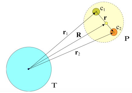
Figure 7: (Color on line) Schematic representation of the colliding system in the 3-body CDCC calculations (figure taken from Ref. Kolinger et al. (2018)). For details, see the text.

U

Let us consider the situation where, during the collision, the projectile breaks up into two fragments without internal structure, $c_{1}$ and $c_{2}$. In this case, the intrinsic coordinate (previously denoted by $\xi$) is the vector joining the centers of the two fragments, ${\bf r}$, as shown in Fig. 7. Along the collision, the target interacts with the fragments through the complex potentials $U_{1}(r_{1})$ and $U_{2}(r_{2})$, which are functions of the moduli of the vectors ${\bf r}_{1}={\bf R}-(A_{2}/A_{\rm\scriptscriptstyle P})\ {\bf r}$ and ${\bf r}_{2}={\bf R}+(A_{1}/A_{\rm\scriptscriptstyle P})\ {\bf r}$, respectively. Thus, the projectile-target interaction is given by

$${\mathbb{U}}({\bf R},{\bf r})=U_{1}(r_{1})+U_{2}(r_{2}).$$ (68)

Then, the total Hamiltonian of the system is

$${\mathbb{H}}({\bf R},{\bf r})=h({\bf r})+\hat{K}+{\mathbb{U}}({\bf R},{\bf r}),$$ (69)

and the scattering state satisfies the Schrödinger equation,

$$\Big{[}E-{\mathbb{H}}\Big{]}\,\left|{\rm\Psi^{\rm\scriptscriptstyle(+)}}\right>=0.$$ (70)

Proceeding as in the case of tightly bound systems, we take scalar product of both sides of the above equation with each of the intrinsic states appearing in the expansions of Eqs. (66) and (67). In this way, we get the sets of coupled equations,

$$\big{[}E-H_{\alpha,\alpha}({\bf R})\big{]}\,\psi_{\alpha}^{\rm\scriptscriptstyle(+)}({\bf R})=\sum_{\alpha^{\prime}}H_{\alpha,\alpha^{\prime}}({\bf R})\,\psi_{\alpha^{\prime}}^{\rm\scriptscriptstyle(+)}({\bf R})\\ +\ \sum_{\beta}\int d\varepsilon\ H_{\alpha,\varepsilon\beta}({\bf R})\,\psi_{\varepsilon\beta}^{\rm\scriptscriptstyle(+)}({\bf R})$$ (71)

and

$$\big{[}E-H_{\varepsilon\beta,\varepsilon\beta}({\bf R})\big{]}\,\psi_{\varepsilon\beta}^{\rm\scriptscriptstyle(+)}({\bf R})=\sum_{\alpha}H_{\varepsilon\beta,\alpha}({\bf R})\,\psi_{\alpha}^{\rm\scriptscriptstyle(+)}({\bf R})\\ +\ \sum_{\beta^{\prime}}\int d\varepsilon^{\prime}\ H_{\varepsilon\beta,\varepsilon^{\prime}\beta^{\prime}}({\bf R})\,\psi_{\varepsilon^{\prime}\beta^{\prime}}^{\rm\scriptscriptstyle(+)}({\bf R}),$$ (72)

where the matrix-elements of the Hamiltonian involving continuum states are defined analogously to Eq. (57). Now, however, the situation is different. This procedure lead to an infinite set of coupled equations, which cannot be solved.

The CDCC method deals with this problem by approximating the infinite dimensional space of scattering states by the reduced space spanned by a finite set of functions. In the simple case where the $c_{1}$ and $c_{2}$ have spin zero, $\beta$ stands for the total angular momentum of the projectile, $j$, and its z-projection, $\nu$. Then, the wave function describing the scattering of the fragments with relative energy $\varepsilon$ can be written as:

$$\varphi_{\varepsilon\beta}({\bf r})=\frac{u_{\varepsilon\beta}(r)}{r}\ \ \mathcal{Y}_{\beta}(\hat{\bf r}),$$ (73)

where $u_{\varepsilon\beta}(r)$ is the radial part of $\varphi_{\varepsilon\beta}({\bf r})$. Above, $\mathcal{Y}_{\beta}(\hat{\bf r})$ is a complementary function of the orientation of ${\bf r}$. The radial wave functions must be normalized to satisfy the relations,

$$\int dr\ u^{*}_{\varepsilon\beta}(r)\ u_{\varepsilon^{\prime}\beta}(r)=\delta(\varepsilon-\varepsilon^{\prime}).$$ (74)

In the particular case of fragments with spin zero, $\beta$ represents the quantum numbers $\{j,\nu\}$. Then, $\mathcal{Y}_{\beta}(\hat{\bf r})\equiv\mathcal{Y}_{jm}(\hat{\bf r})$ are the usual spherical harmonics. In more general situations, it is a more complicated function Druet et al. (2010); Thompson and Nunes (2009); Canto and Hussein (2013), involving spherical harmonics, spin states and angular momentum coupling coefficients.

The CDCC approximation consists in replacing the infinite integral over $\varepsilon$ by the sum

$$\int\ d\varepsilon\ \frac{u_{\varepsilon\beta}(r)}{r}\ \longrightarrow\ \sum_{n=1}^{n_{\rm max}}\ \frac{\phi_{n\beta}(r)}{r},$$ (75)

where the set of $n_{\rm max}$ functions $\phi_{n\beta}(r)$ must satisfy the orthonormality relations

$$\int\ d\varepsilon\ \phi^{*}_{n\beta}(r)\ \phi_{n^{\prime}\beta}(r)=\delta_{nn^{\prime}}.$$ (76)

Further, the intrinsic hamiltonian should be diagonal in the $n_{\rm\scriptscriptstyle max}$ dimensional space of the functions $\phi_{n\beta}(r)$. That is

$$\left\langle\phi_{n\beta}\,\right|\ h\ \left|\,\phi_{n^{\prime}\beta}\right\rangle=\bar{\varepsilon}_{n}\ \delta_{nn^{\prime}}.$$ (77)

Otherwise, there would be channel couplings even without the interaction with the target.

With the continuum discretization of Eq. (75), bound and unbound states can be treated on the same grounds. Then, the infinite set of Eqs. (71) and (72) reduces to a finite set of equations with the general form of Eq. (56). Now, however, $\alpha$ stands for any state of the projectile, bound or unbound. The number of coupled equations, $N$, is given by

$$N=N_{\rm\scriptscriptstyle B}+N_{\rm\scriptscriptstyle C},$$ (78)

where $N_{\rm\scriptscriptstyle B}$ and $N_{\rm\scriptscriptstyle C}$ are respectively the number of bound and continuum-discretized states of the projectile. The latter is given by

$$N_{\rm\scriptscriptstyle C}=n_{\rm\scriptscriptstyle max}\times\beta_{\rm\scriptscriptstyle max}.$$ (79)

In practice, the number of coupled equation is much smaller than $N$. When proper angular momentum projections are carried out, and angular momentum, and parity conservations are taken into account, the set of equations splits into decoupled sets of smaller dimensions, one for each invariant sub-space.

The discretization of the continuum may be performed by two methods: the bin method and the method of pseudo-states. These methods are briefly discussed below.

a) The bin method

In the bin method, the functions $\phi_{n\beta}(r)$ are generated by scattering states of the fragments through wave packets with the general form,

$$\phi_{n\beta}(r)=\int d\varepsilon\ \Gamma_{n}(\varepsilon)\,u_{\varepsilon\beta}(r),$$ (80)

with the weight function, $\Gamma_{n}(\varepsilon)$, concentrated around $\varepsilon_{n}$.

The most common weight functions used in nuclear physics are constant within some limited energy interval, and zero elsewhere Sakuragi et al. (1986); Austern et al. (1987); Matsumoto et al. (2003); Thompson and Nunes (2009). The continuum is truncated at some energy $\varepsilon_{\rm\scriptscriptstyle max}$ and the interval from 0 to the cut-off energy is divided into a set of non-overlapping intervals $\Delta_{m}$, centered at the energy $\varepsilon_{m}$, such that the upper limit of each interval coincides with the lower limit of the subsequent one. That is,

$$\Gamma_{m}(\varepsilon) = \frac{1}{\sqrt{\Delta_{m}}},\qquad{\rm if}\ \varepsilon_{m}^{\rm\scriptscriptstyle(+)}\geq\varepsilon_{m}\geq\varepsilon_{m}^{\rm\scriptscriptstyle(-)}$$ (81)

$$= 0,\qquad\qquad{\rm otherwise},$$

where $\varepsilon_{m}^{\rm\scriptscriptstyle(\pm)}=\varepsilon_{m}\pm\Delta_{m}/2$ are the limits of the interval. The most common choice is to use bins of constant width in momentum space. In this case, the energy width increase linearly with $k$. On the other hand, when there are sharp resonances in the scattering of the fragments, it is necessary to reduce the width and increase the density of bins around the resonance.

In most CDCC calculations the discretization is carried out with bins in momentum space, labeled by $k=\sqrt{2\mu_{\rm\scriptscriptstyle 12}\varepsilon}/\hbar$, where $\mu_{\rm\scriptscriptstyle 12}$ is the reduced mass in the $c_{1}-c_{2}$ collision. In this case, the bins are given by

$$\phi_{m\beta}(r)=\int dk\ \Gamma_{m}(k)\,u_{k\beta}(r),$$ (82)

with the scattering states satisfying the orthonormality relations

$$\int dr\ u^{*}_{k\beta}(r)\ u_{k^{\prime}\beta}(r)=\frac{\pi}{2}\ \delta(k-k^{\prime}).$$ (83)

The constant weight functions now are given by

$$\Gamma_{m}(k) = \frac{1}{\sqrt{\Delta_{m}}},\qquad{\rm if}\ k_{m}^{\rm\scriptscriptstyle(+)}\geq k_{m}\geq k_{m}^{\rm\scriptscriptstyle(-)}$$ (84)

$$= 0,\qquad\qquad{\rm otherwise},$$

with $k_{m}^{\rm\scriptscriptstyle(\pm)}=k_{m}\pm\Delta_{m}/2$, and $\Delta_{m}$ now has the dimension of $p/\hbar$. Since the energy is proportional to $k^{2}$, the energy width of a bin with constant width in $k$-space increases linearly with $k$.

It can be easily proved that the functions generated by the weight functions of Eq. (81) form an orthonormal set. For this purpose, we take the scalar product of two bins and use the orthonormality of the scattering states (Eq. (74)). We get,

$$\left\langle\phi_{n\beta}\,|\,\phi_{n^{\prime}\beta}\right\rangle=\int d\varepsilon\ \Gamma_{n}(\varepsilon)\,\Gamma_{n^{\prime}}(\varepsilon)=\delta_{n,n^{\prime}}.$$ (85)

The second equality in the above equation was obtained inserting the weight functions of Eq. (81) into the integral over $\varepsilon$. It is equally straightforward to show that the intrinsic Hamiltonian is diagonal in this bin space. Proceeding similarly, one gets

$$\left\langle\phi_{n\beta}\,|\,h\,|\,\phi_{n^{\prime}\beta}\right\rangle=\int d\varepsilon\ \Gamma_{n}(\varepsilon)\ \varepsilon\ \Gamma_{n^{\prime}}(\varepsilon)=\bar{\varepsilon}_{n}\ \delta_{n,n^{\prime}}.$$ (86)

The weight functions of Eq. (81) are very easy to handle but the abrupt change at the edges leads to bins with longer ranges and with beats at large radial distances Bertulani and Canto (1992). Although it is not a serious problem, it can be avoided with smooth weight functions, as the ones proposed in Ref. Bertulani and Canto (1992), and used in Refs. Bertulani and Canto (1992); Marta et al. (2008, 2014); Kolinger et al. (2018). However, there is a drawback with these weight functions: they do not diagonalize the intrinsic Hamiltonian. It is then necessary to perform a unitary transformation in the bin space,

$$\phi_{n\beta}(r)\ \rightarrow\ \bar{\phi}_{n\beta}(r)=\sum_{n=1}^{n_{\rm\scriptscriptstyle max}}U_{nm}(\beta)\ \phi_{m\beta}(r),$$ (87)

with the operator $U(\beta)$ determined by the condition

$$\left<\bar{\phi}_{nj}\right|h\left|\bar{\phi}_{n^{\prime}j}\right>=\sum_{m,m^{\prime}=1}^{n_{\rm\scriptscriptstyle max}}U^{\dagger}_{nm}(\beta)\ h_{mm^{\prime}}\ U_{m^{\prime}n^{\prime}}(\beta)=\bar{\varepsilon}_{n}\ \delta_{n,n^{\prime}},$$ (88)

where

$$h_{mm^{\prime}}=\left<\phi_{m\beta}\right|h\left|\phi_{m^{\prime}\beta}\right>.$$ (89)

b) The pseudo-states method

In the pseudo-states (PS) method, the space of scattering states is approximated by a finite dimensional space spanned by a set of square-integrable functions. These functions are approximate eigenstates of $h$ with positive energy. The method is developed in two steps. First, one selects a set of square integrable functions $\phi_{m\beta}(r)$. Then, the pseudo-states, $\bar{\phi}_{n\beta}(r)$, are determined by diagonalizing $h$ in this space spanned by this set. The diagonalization is performed as in the case of non-orthogonal bins, following the procedure of Eqs. (87), (88) and (89). There is, however, a difference. In the bin method, the functions $\phi_{m\beta}(r)$ are wave packets of scattering states. Thus, the eigenvalues $\bar{\varepsilon}_{n}$ are all positive. Now the situation is different. There are also negative eigenvalues, which represent the bound states of the projectile. In most cases, these states are calculated directly, without expansion in PC basis. In such cases, the eigenstates with negative energy obtained through the diagonalization of $h$ should be discarded.

The choice of square-integrable set of states, $\phi_{n\beta}(r)$, is arbitrary, provided that they give a good description of the radial wave functions, within the range of the coupling interactions. Choices based on Gaussian functions are extensively discussed in Ref. Hiyama et al. (2003). We mention two of them. The first is the set of $N$ real Gaussian functions with variable range Matsumoto et al. (2003),

$$\phi_{n\beta}(r)=r^{l_{\beta}}\ \exp\left[-\,r^{2}/a_{n}^{2}\right],$$ (90)

where $l_{\beta}$ is the orbital angular momentum of the $c_{1}-c_{2}$ relative motion in the state $\phi_{n\beta}$. The range increases from $a_{1}$ to $a_{\rm\scriptscriptstyle N}$, in the geometrical progression

$$a_{n}=a_{1}\ \left(\frac{a_{\rm\scriptscriptstyle N}}{a_{1}}\right)^{(n-1)/(N-1)},$$ (91)

where $a_{1}$ and $a_{\rm\scriptscriptstyle N}$ are parameters of the set. The second is a set of $2N$ functions obtained by the multiplication of the Gaussians of Eq. (90) by oscillating functions, in the form Hiyama et al. (2003),

$$\phi^{\rm\scriptscriptstyle C}_{n\beta} = \phi_{n\beta}\ \cos\left[b\,(r/a_{n})\right]$$ (92)

$$\phi^{\rm\scriptscriptstyle S}_{n\beta} = \phi_{n\beta}\ \sin\left[b\,(r/a_{n})\right],$$ (93)

where $b$ is an adjustable parameter. This set corresponds to taking the real and the imaginary parts of the functions of Eq. (90) with complex widths. Calculations using this set of states converge more rapidly than the ones using the Gaussians of Eq. (90).

Some CDCC calculations adopting the Lagrange-mesh method make a different choice of basis functions. In such cases, one frequently uses basis functions associated with a Gauss quadrature Hesse et al. (1998); Druet et al. (2010). This greatly simplifies the numerical calculations.

A large number of three-body CDCC calculations neglecting excitations of the fragments and the target have been reported. For a review, see, e.g. Refs. Canto et al. (2015a); Sakuragi et al. (1986); Austern et al. (1987).

Core and target excitations

Until recently, the available CDCC calculations ignored intrinsic structures of the projectile’s fragments and of the target, treating them as point particles. Frequently, these approximations are reasonable. However, the neglected degrees of freedom may play an important role in the reaction dynamics of some colliding systems. Formally, the inclusion of excitations of the fragments or of the target is straightforward. However, from the computational point of view it is not a trivial task. Usually, the calculations are performed by standard computer codes available in the literature and the inclusion of fragment or target excitation involves modifications that requires considerable knowledge of the structure of the code. In addition, the inclusion of these excitations enlarges significantly the dimension of the matrices involved in the calculations, demanding much more computer power. Calculations with excitations of one of the fragments or of the target will be briefly discussed below (we follow Ref. Moro and Gómez-Camacho (2016)).

a) CDCC with Core excitation (XCDCC)

If the intrinsic structure of a projectile fragment, say $c_{1}$, with coordinates $\xi_{1}$, is taken into account, the total Hamiltonian of the system becomes

$${\mathbb{H}}({\bf R};{\bf r},\xi_{1})=h({\bf r},\xi_{1})+\hat{K}+{\mathbb{U}}({\bf R};{\bf r},\xi_{1}),$$ (94)

with the projectile-target potential

$${\mathbb{U}}({\bf R};{\bf r},\xi_{1})=U_{1}({\bf r}_{1},\xi_{1})+U_{2}(r_{2}).$$ (95)

Above, $\xi_{1}$ stands for the intrinsic coordinates of fragment $c_{1}$. Then, the projectile’s wave functions of Eq. (73) takes the form

$$\varphi_{\varepsilon\beta}({\bf r})=\frac{u_{\varepsilon\beta}(r)}{r}\ \ \mathcal{Y}_{\beta}(\hat{\bf r},\xi_{1}).$$ (96)

Now the index $\beta$ stands for angular momenta of the projectile and the fragments, and also for the quantum numbers associated with the degrees of freedom represented by $\xi_{1}$.

This generalization of the CDCC approximation, known as XCDCC, was introduced by Summers et al. Summers et al. (2006); Summers and Nunes (2007), to study the breakup of ${}^{17}{\rm C}$ (${}^{16}{\rm C}+p$) and ${}^{11}{\rm Be}$ (${}^{10}{\rm Be}+n$) projectiles on ⁹Be targets. The calculations included excitation channels related to rotational bands of the deformed ¹⁶C and ¹⁰Be cores.

More recently, similar calculations have been carried out to study different reactions. Moro and Crespo Moro and Crespo (2012) studied the influence of rotational excitations of the deformed ¹⁰Be core in the breakup of ¹¹Be (${}^{10}{\rm Be}+n$) projectiles in collisions with a proton target. For this purpose, they proposed a simple reaction model using the DWBA.

De Diego et al. de Diego et al. (2014) used a more realistic XCDCC model to evaluate quasi-elastic and breakup cross sections for the same system, at collision energies ranging from 10 to 200 MeV/nucleon.

Chen et al. Chen et al. (2016) measured elastic and breakup cross sections for the same ${}^{11}{\rm Be}+p$ system at 26.9 MeV/nucleon, and compared the data with results of CDCC and XCDCC calculations including rotational excitations of ¹⁰Be. They concluded that excitations of the core play a moderate role in the reaction dynamics.

Later on, De Diego et al. de Diego et al. (2017) performed similar XCDCC calculations, to evaluate cross sections for different two- and three-body observables, at different collision energies, for which there are data available. In this way, they investigated the importance of core excitation in the reaction dynamics.

Figure 8: (Color on line) Elastic angular distribution in the ¹¹Be + ¹⁹⁷Au collision at two collision energies, divided by the corresponding Rutherford cross sections. Results of XCDCC (solid line) and CDCC (dashed line) are compared to the experimental data. The figure, the data and the calculations are from Ref. Pesudo et al. (2017).

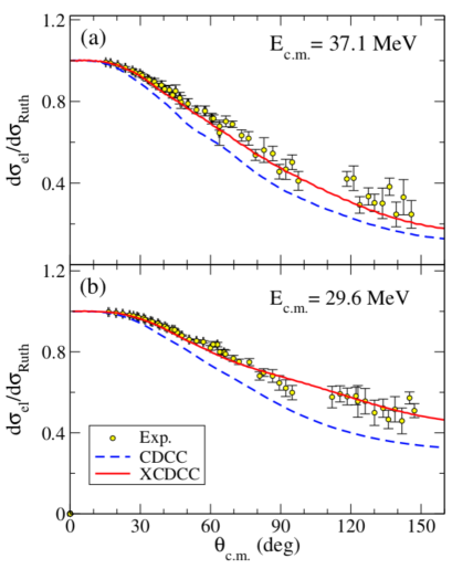
Figure 9: (Color on line) Similar to the previous figure, but for breakup angular distributions (figure extracted from Ref. Pesudo et al. (2017)).

Pesudo et al. Pesudo et al. (2017) measured elastic scattering, inelastic scattering and breakup in collisions of ¹¹Be projectiles with a heavy target. They studied the ${}^{11}{\rm Be}\,-\,^{197}$Au collision at two energies, below and around the Coulomb barrier. The experimental cross sections were then compared with predictions of CDCC and XCDCC calculations. Their elastic and breakup cross sections are shown in Figs. 8 and 9, respectively. The elastic scattering data is well reproduced by the XCDCC calculations, whereas the predictions of the standard CDCC calculations fall systematically below the data. This clearly indicates the importance of the core excitation for a proper description of the reaction dynamics of this system. On the other hand, inspecting Fig. 9, one concludes that the inclusion of core excitations in the calculations of breakup cross sections is not as important as in the case of elastic scattering.

Lay et al. Lay et al. (2016) performed XCDCC calculations for ${}^{19}{\rm C}+p$ system, to analyse the resonant breakup of ¹⁹C, which has been measured at RIKEN Satou et al. (2008). The inclusion of core excitation was shown to be essential for a good description of the data. CDCC calculations with an inert core largely underestimated the data.

b) CDCC with excitations of the target

If the intrinsic degrees of freedom of the target, $\xi_{\rm\scriptscriptstyle T}$ are taken into account, the system’s Hamiltonian becomes,

$${\mathbb{H}}({\bf R};{\bf r},\xi_{\rm\scriptscriptstyle T})=h({\bf r})+H_{\rm\scriptscriptstyle T}(\xi_{\rm\scriptscriptstyle T})+\hat{K}+{\mathbb{V}}({\bf R};{\bf r};\xi_{\rm\scriptscriptstyle T}),$$ (97)

with

$${\mathbb{V}}({\bf R};{\bf r};\xi_{\rm\scriptscriptstyle T})=V_{1}({\bf r}_{1},\xi_{\rm\scriptscriptstyle T})+V_{2}({\bf r}_{2},\xi_{\rm\scriptscriptstyle T}).$$ (98)

In this case, the label $\beta$ stands also for quantum numbers of the target, and Eq. (73) becomes

$$\varphi_{\varepsilon\beta}({\bf r})=\frac{u_{\varepsilon\beta}(r)}{r}\ \ \mathcal{Y}_{\beta}(\hat{\bf r},\xi_{\rm\scriptscriptstyle T}).$$ (99)

The importance of target excitations in weakly bound systems has been investigated by Lubian et al. Lubian et al. (2009). They performed CDCC calculations for the ${}^{9}{\rm Be}\,+\,^{58}{\rm Ni}$ system, including and not including excitations of the target. Comparing their results to the data of Aguilera et al. Aguilera et al. (2009a), they concluded that the inclusion of continuum states was essential to describe the data, whereas the influence of target excitations was weak.

Woodward et al. Woodward et al. (2012) performed CDCC calculations for the ${}^{6}{\rm Li}+^{144}{\rm Sm}$ system. Besides the continuum space of the projectile, the calculations took into account the excitation of the $2^{+}_{1}$ and $3^{-}_{1}$ states in ¹⁴⁴Sm. Inelastic angular distributions populating the two excited states of the target have been measured at near-barrier energies, and the results were compared with the predictions of standard coupled channel calculations and with their CDCC calculations with target excitation. This study lead to the conclusion that a full treatment of the continuum, including continuum-continuum couplings, is essential for a good description of the data.

Gómez-Ramos and Moro Gómez-Ramos and Moro (2017) developed a comprehensive study of the influence of the breakup channel on excitations of the target, in collisions with weakly bound projectiles. They performed standard coupled channel and CDCC calculations with target excitation for the following reactions:

${}^{58}{\rm Ni}(d,d)^{58}{\rm Ni}^{*}$, ${}^{24}{\rm Mg}(d,d)^{24}{\rm Mg}^{*}$, ${}^{144}{\rm Sm}(^{6}{\rm Li},^{6}{\rm Li})^{144}{\rm Sm}^{*}$, ${}^{9}{\rm Be}(^{6}{\rm Li},^{6}{\rm Li})^{9}{\rm Be}^{*}$.

They obtained a satisfactory agreement with the data for both, standard and target excitation calculations, and concluded that the continuum had a moderate influence in the inelastic scattering.

Four-body CDCC

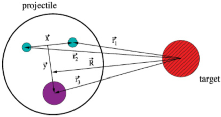
Figure 10: (Color on line) Coordinates used in four-body CDCC calculations, where the projectile breaks up into three fragments (figure taken from Ref. Rodríguez-Gallardo et al. (2008)).

Owing to their cluster configuration, several weakly bound nuclei can break up into three fragments during a collision. Important examples are the stable ⁹Be (${}^{4}{\rm He}+^{4}{\rm He}+n$) and radioactive two neutron halo nuclei, like ⁶He (${}^{4}{\rm He}+n+n$) and ¹¹Li (${}^{9}{\rm Li}+n+n$). Thus, in collisions of projectiles with this configuration, the reaction dynamics involves four particles: the three clusters of the projectile, and the target. This calls for a generalization of the CDCC method, usually called four-body CDCC (to distinguish these methods, we henceforth adopt the notations 3b-CDCC and 4b-CDCC).

A collision of a three-fragment projectile with a target is schematically represented in Fig. 10. The projectile-target interaction is the sum of interactions between the fragments and the target, $U_{c_{i}-T}\,(i=1,3)$, which depend on the fragment-target coordinates ${\bf r}_{i}$, shown in Fig. 10. These coordinates are usually expressed in terms of the Jacobi coordinates, defined as

$${\bf x} = \sqrt{\frac{A_{\rm\scriptscriptstyle 1}A_{\rm\scriptscriptstyle 2}}{A_{\rm\scriptscriptstyle 1}+A_{\rm\scriptscriptstyle 2}}}\ \left({\bf r}_{\rm\scriptscriptstyle 2}-{\bf r}_{\rm\scriptscriptstyle 3}\right),$$ (100)

$${\bf y} = \sqrt{\frac{A_{\rm\scriptscriptstyle 3}\,\left(A_{\rm\scriptscriptstyle 1}+A_{\rm\scriptscriptstyle 2}\right)}{A_{\rm\scriptscriptstyle P}}}\ \left[{\bf r}_{\rm\scriptscriptstyle 3}-\frac{A_{\rm\scriptscriptstyle 1}\,{\bf r}_{\rm\scriptscriptstyle 1}+A_{\rm\scriptscriptstyle 2}\,{\bf r}_{\rm\scriptscriptstyle 2}}{A_{\rm\scriptscriptstyle 1}+A_{\rm\scriptscriptstyle 2}}\right].$$ (101)

The Hamiltonian of the projectile-target system then reads

$$\mathbb{H}({\bf R};{\bf x},{\bf y})=h({\bf x},{\bf y})+\hat{K}+\mathbb{U}({\bf R};{\bf x},{\bf y}),$$ (102)

where $\mathbb{U}({\bf R};{\bf x},{\bf y})$ is the sum of the three complex fragment-target interactions, expressed in terms of the Jacobi coordinates.

The system’s wave functions still have the general form of Eq. (73), but with $\beta$ representing a larger number of intrinsic quantum numbers, and with the replacement,

$$\mathcal{Y}_{\beta}(\hat{\bf r})\rightarrow\mathcal{Y}_{\beta}({\bf x},{\bf y}).$$

4b-CDCC calculations have been performed to evaluate several observables in different collisions of weakly bound nuclei. Matsumoto et al. Matsumoto et al. (2004) performed 3b- and 4b-CDCC calculations of elastic angular distributions in ${}^{6}{\rm Li}-^{12}{\rm C}$ scattering.

Rodríguez-Gallardo et al. Rodríguez-Gallardo et al. (2008) performed 4b-CDCC calculations of elastic angular distributions for ⁶He projectiles on ¹²C, ⁶⁴Zn and ²⁰⁸Pb targets.

Cubero et al. Cubero et al. (2012) measured elastic angular distributions for ¹¹Li projectiles on a ²⁰⁸Pb target, at two energies around the Coulomb barrier. The data exhibited a strong damping at small angles, even at the energy below the barrier. This behaviour can be traced back to the breakup of the two-neutro-halo projectile, under the action of the long-range dipole interaction. The authors performed 4b-CDCC calculations, and compared the resulting cross sections with the data. The agreement between theory and experiment was very good.

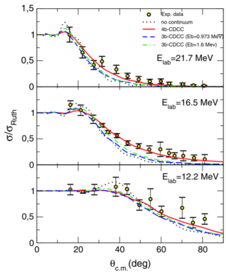
Figure 11: (Color on line) Experimental elastic angular distribution in the ⁶He + ⁵⁸Ni collision at three energies, in comparison with predictions of 3-body and 4-body CDCC calculations Morcelle et al. (2014a).

Morcelle et al. Morcelle et al. (2014a) measured elastic angular distributions in collisions of ⁶He projectiles with a ⁵⁸Ni target, at three near-barrier energies. The results are shown in Fig. 11, in comparison with predictions of 3b- and 4b-CDCC calculations. Clearly, the predictions of 4b-CDCC are much closer to the data than those of 3b-CDCC, mainly at $E_{\rm lab}=16.5$ MeV.

Descouvemont et al. Descouvemont et al. (2015) performed four-body CDCC calculations for the ${}^{9}{\rm Be}+^{209}{\rm Bi}$ system. Elastic scattering, breakup and total fusion cross sections were evaluated simultaneously. The results were shown to be in good agreement with the data.

Fernández-García et al. Fernández-García et al. (2019) measured elastic angular distributions and cross sections for the production of ${}^{4}{\rm He}$, in the ${}^{6}{\rm He}-^{64}$Zn collision. They performed coupled reaction channel (CRC), 3b-CDCC and 4b-CDCC calculations, and compared the resulting cross sections with the data. They found that the elastic cross sections of 3b-CDCC (using the di-neutron model) and 4b-CDCC are very similar, and close to the data. On the other hand, the contribution from elastic breakup to the ${}^{4}{\rm He}$ production cross section is very small. Although CRC calculations of 2n transfer gave a reasonable description of the data, inclusive cross section obtained with the Ichimura, Austern and Vincent (IAV) model Ichimura et al. (1985); Austern et al. (1987) are closer to the experiment.

A very nice example where 4b-CDCC reproduces the data much better than 3b-CDCC is shown in Fig. 12. Although the two CDCC calculations reproduce equally well the data at backward angles, the 4b-CDCC cross section remains close to it at forward angles, whereas the 3b-CDCC cross section falls significantly below.

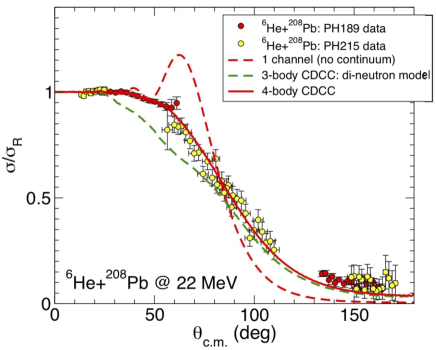
Figure 12: (Color on line) Experimental angular distribution in ${}^{6}{\rm He}\,+\,^{208}$Pb elastic scattering, in comparison with predictions of theoretical models. The data denoted by PH189 and PH215 are respectively from Refs. Sánchez-Benítez et al. (2008) and Acosta et al. (2011a), the 1-channel and the 3b-CDCC calculations are from Ref. Moro et al. (2007), and the 4b-CDCC calculations are from Ref. Rodríguez-Gallardo et al. (2009) (figure taken from a private communication with A. Moro).

Other generalizaions of the CDCC

Recently, Pierre Descouvemont introduced two generalizations of the CDCC method. The first Descouvemont and Itagaki (2018) is to use microscopic wave functions in a multi-cluster model ($\alpha+\alpha+n$) for the bound states of ⁹Be. This treatment has the nice feature of being based exclusively on nucleon-target interactions. The model was applied to the ${}^{9}{\rm Be}\,+\,^{208}{\rm Pb}$ and ${}^{9}{\rm Be}\,+\,^{27}{\rm Al}$ systems, and the results were shown to be in fair agreement with the data.

The second generalization Descouvemont (2017); Desc (2018) is an extension of the 4b-CDCC approach to deal with collisions between two weakly bound nuclei, when each one can break up into two fragments. The new reaction model was applied to the ${}^{11}{\rm Be}-d$ collision at $E_{\rm c.m.}=45.5$ MeV. It was shown that for a good description of the elastic scattering data it is necessary to consider continuum states of the two collision partners simultaneously.

4 Hybrid reactions: The Surrogate Method

With the advent of secondary beams of unstable nuclei one is bound to deal with reaction cross sections of only a piece of the projectile. Further, some of the desired reactions can not be measured in the laboratory even in the case of stable projectiles. Thus one has to find a way to extract the desired cross section from a measurement of the spectrum of the observed piece of the primary projectile. An example, is deuteron-induced reaction of the type $(d,p)$ where the neutron is captured by a target such as ²³⁸U or ²³²Th of importance for nuclear energy generation in fast breeder reactions. The measured proton spectrum can then be used to extract cross sections for neutron capture reactions, like: $n+^{238}{\rm U}\rightarrow\,^{239}{\rm U}$ or $n+^{232}{\rm Th}\rightarrow\,^{233}$Th. The method used to extract the desired neutron capture cross sections is referred to as the Surrogate Method (SM). Even in cases where the primary projectile is a weakly bound two-cluster projectile such as ${}^{6}{\rm Li}=\,^{4}{\rm He}+d$, the measurement of the deuteron spectrum will supply information on the alpha capture by the target. This represents the incomplete fusion of the projectile, which when added to the complete fusion supplies the total fusion. Therefore, as part of this review it is important to give an account of the theory which supplies the expression of the spectrum of the detected fragment, and exhibit how this spectrum is directly proportional to the secondary reaction cross section (the desired cross section). The primary reaction cross section of the full projectile is of course extracted as discussed in the previous section, and relies on the careful measurement of the angular distribution of the elastic scattering.

The theory that we summarise below is the inclusive nonelastic breakup theory (NEB). Let us first deal with the reaction $A\,(d,p)\,B$, where $B=A+n$. The NEB cross section for the emerging proton at an angle $\theta_{p}$ and with energy $E_{p}$ is

$$\frac{d^{2}\sigma^{\rm\scriptscriptstyle NEB}_{p}}{dE_{p}\,d\Omega_{p}}=\rho_{p}(E_{p})\ \bar{\sigma}_{\rm\scriptscriptstyle R}^{{\rm n}{\rm\scriptscriptstyle A}},$$ (103)

where $\rho_{p}(E_{p})$ is the density of proton states and $\bar{\sigma}_{{\rm\scriptscriptstyle R}}^{{\rm n}{\rm\scriptscriptstyle A}}$ is the medium-modified total reaction cross section in the collision between the neutron and the target.

The Surrogate Method (SM) purports to extract $\bar{\sigma}_{\rm\scriptscriptstyle R}^{n}$ through a measurement of $d^{2}\sigma_{p}/dE_{p}\,d\Omega_{p}$. In fact, what is done is a measurement of the protons in coincidence with one decay product of the secondary compound nucleus $B=A+n$ Hussein (2017). Several publications on the SM have recently appeared Escher et al. (2012). Very recently this method was employed to populate the compound nucleus involving radioactive targets Potel et al. (2017).

4.1 The inclusive nonelastic breakup cross section

In the more general case of a two-cluster primary projectile, $a=b+x$, the NEB theory gives for the $a+A\rightarrow b+B$ (with $B=x+A$) reaction cross section,

$$\frac{d^{2}\sigma^{\rm\scriptscriptstyle NEB}_{b}}{dE_{b}\,d\Omega_{b}}=\rho_{b}(E_{b})\ \bar{\sigma}_{\rm\scriptscriptstyle R}^{{\sc x}{\rm\scriptscriptstyle A}}\ ,$$ (104)

where $\bar{\sigma}_{\rm\scriptscriptstyle R}^{{\sc x}{\rm\scriptscriptstyle A}}$ is the total reaction cross section of the interacting fragment, $x$, on the target and

$$\rho_{b}(E_{b})\equiv\frac{1}{(2\pi)^{3}}\ \frac{d^{3}{\bf k}_{b}}{dE_{b}\,d\Omega_{b}}=\frac{\mu_{b}\,k_{b}}{8\pi^{3}\,\hbar^{2}}$$ (105)

is the density of states of the observed fragment, $b$. We consider the situation where $a$ is much lighter than $A$, so that one can assume the target has infinite mass.

In this section we discuss the calculation of the NEB cross section within different participant-spectator models, following the work of Ichimura Ichimura (1990) (a recent review on this topic, can be found in Ref. Potel et al. (2017)). They all lead to an expression of the form

$$\frac{d^{2}\sigma^{\rm\scriptscriptstyle NEB}_{b}}{dE_{b}\,d\Omega_{b}}=-\,\frac{2}{v_{a}}\,\rho(E_{b})\,\left\langle\varphi_{x}\right|\,W_{xA}\,\left|\varphi_{x}\right\rangle,$$ (106)

where $W_{xA}$ is the imaginary part of an effective potential $U_{xA}$, which will be derived below, and $\varphi_{x}$ is is the so called source function, which varies according to the particular implementation of the model. The starting point is the system Hamiltonian,

$$H=K_{b}+K_{x}+h_{\sc A}(\xi)+V_{bx}+V_{xA}+U_{bA},$$ (107)

where $K_{b}$ and $K_{x}$ are respectively the kinetic energy operators of particles $b$ and $x$, $h_{\sc A}$ is the intrinsic Hamiltonian of the target, $V_{bx}$ and $V_{xA}$ are respectively real potentials representing the interactions of $x$ with $b$ and $A$, and $U_{bA}$ is the complex optical potential between particle $b$ and the target. The intrinsic structures of $b$ and $x$ are neglected, whereas the target has a set of intrinsic states satisfying the equation,

$$h_{A}\,\phi_{\alpha}(\xi)=\varepsilon_{\alpha}\,\phi_{\alpha}(\xi).$$ (108)

We are interested in final states in the form

$$\left|\chi^{\rm\scriptscriptstyle(-)}_{{\bf k}_{b}}\,{\rm\Phi}_{\alpha}^{\rm\scriptscriptstyle(-)}\right>\equiv\left|\chi^{\rm\scriptscriptstyle(-)}_{{\bf k}_{b}}\right)\otimes\left|{\rm\Phi}_{\alpha}^{\rm\scriptscriptstyle(-)}\right),$$ (109)

where $\left|\chi^{\rm\scriptscriptstyle(-)}_{{\bf k}_{b}}\right)$ is a distorted wave with momentum $\hbar{\bf k}_{b}$ with ingoing wave boundary condition, satisfying the equation

$$\left[K_{b}+U^{\dagger}_{bA}-E_{b}\right]\left|\chi^{\rm\scriptscriptstyle(-)}_{{\bf k}_{b}}\right)=0,$$ (110)

and $\left|{\rm\Phi}_{\alpha}^{\rm\scriptscriptstyle(-)}\right)$ is a scattering state of the $x+A$ system with ingoing wave boundary condition, satisfying the equation

$$\left[H_{xA}-E_{\alpha}\right]\left|{\rm\Phi}_{\alpha}^{\rm\scriptscriptstyle(-)}\right)=0.$$ (111)

Above, $E_{\alpha}=E-E_{b}$ and

$$H_{xA}=h_{\rm\scriptscriptstyle A}+K_{x}+V_{xA}.$$ (112)

is the Hamiltonian of the $x+A$ system. Then, the corresponding T-matrix in the post representation is

$$T_{\alpha{\bf k}_{b}}=\left\langle\chi^{\rm\scriptscriptstyle(-)}_{{\bf k}_{b}}\,{\rm\Phi}_{\alpha}^{\rm\scriptscriptstyle(-)}\right|\,V_{bx}\,\left|{\rm\Psi}^{\rm\scriptscriptstyle(+)}\right\rangle,$$ (113)

where $\left|{\rm\Psi}^{\rm\scriptscriptstyle(+)}\right\rangle$ is the scattering wave function, which satisfies the Schrödinger equation with the full Hamiltonian of Eq. (107), namely

$$\left[H-E\right]\left|{\rm\Psi}^{\rm\scriptscriptstyle(+)}\right\rangle=0.$$ (114)

The inclusive breakup cross section is given in terms of the T-matrix by the expression (see e.g. Eq.(1.31) of Ref. Rodberg and Thaler (1967))

$$\frac{d^{2}\sigma^{\rm inc}_{b}}{dE_{b}\,d\Omega_{b}}=\frac{2\pi}{v_{a}}\ \rho_{b}(E_{b})\ \sum_{\alpha}\left|T_{\alpha{\bf k}_{b}}\right|^{2}\ \delta\left(E-E_{b}-E_{\alpha}\right),$$ (115)

where $v_{a}$ is the incident velocity of $a$. Using in Eq. (115) the well known identity

$$\frac{1}{x+i\epsilon}={\mathcal{P}}\left\{\frac{1}{x}\right\}-i\pi\,\delta(x),$$ (116)

with ${\mathcal{P}}$ standing for the principal value, and replacing $T_{\alpha{\bf k}_{b}}$ by its explicit form ((Eq. (113)), the inclusive breakup cross section becomes

$$\frac{d^{2}\sigma^{\rm inc}_{b}}{dE_{b}\,d\Omega_{b}}=-\frac{2}{v_{a}}\ \rho_{b}(E_{b})\ {\rm Im}\Big{\{}\big{\langle}{\rm\Psi}^{\rm\scriptscriptstyle(+)}\big{|}\,V_{bx}\big{|}\chi_{{\bf k}_{b}}^{\rm\scriptscriptstyle(-)}\big{)}\\ \Big{[}\sum_{\alpha}\big{(}{\rm\Phi}_{\alpha}^{\rm\scriptscriptstyle(-)}\big{|}\,\frac{1}{E-E_{b}-E_{\alpha}+\i\epsilon}\big{|}{\rm\Phi}_{\alpha}^{\rm\scriptscriptstyle(-)}\big{)}\ \Big{]}\\ \big{(}\chi_{{\bf k}_{b}}^{\rm\scriptscriptstyle(-)}\big{|}\,V_{bx}\big{|}{\rm\Psi}^{\rm\scriptscriptstyle(+)}\big{\rangle}\Big{\}}.$$ (117)

The quantity within square brackets in the above equation is the spectral representation of the Green’s function associated with the Hamiltonian of Eq. (112), $G^{\rm\scriptscriptstyle(+)}_{xA}(E-E_{b})$. Then, we can write

$$\frac{d^{2}\sigma^{\rm inc}_{b}}{dE_{b}\,d\Omega_{b}}=-\frac{2}{v_{a}}\ \rho_{b}(E_{b})\ {\rm Im}\Big{\{}\big{\langle}{\rm\Psi}^{\rm\scriptscriptstyle(+)}\big{|}\,V_{bx}\big{|}\chi_{{\bf k}_{b}}^{\rm\scriptscriptstyle(-)}\big{)}\\ G^{\rm\scriptscriptstyle(+)}_{xA}(E-E_{b})\ \big{(}\chi_{{\bf k}_{b}}^{\rm\scriptscriptstyle(-)}\big{|}\,V_{bx}\big{|}{\rm\Psi}^{\rm\scriptscriptstyle(+)}\big{\rangle}\Big{\}}.$$ (118)

Different approximations have been adopted for the exact wave function $\left|{\rm\Psi}^{(+)}\right\rangle$. Some of them are discussed below.

The three-body model

First, we consider the approximation of $\left|{\rm\Psi}^{(+)}\right\rangle$ by the three-body wave function of Austern et al. Austern et al. (1987),

$$\big{|}{\rm\Psi}^{\rm\scriptscriptstyle(+)}\big{\rangle}\sim\big{|}{\rm\Psi}^{\rm\scriptscriptstyle(+)}_{3b}\big{\rangle}=\big{|}{\rm\psi}^{\rm\scriptscriptstyle(+)}_{3b}\big{)}\otimes\big{|}\phi_{0}\big{)},$$ (119)

where $\left|\phi_{0}\right)\equiv\left|\phi_{\alpha=0}\right)$ is the ground state of the target. Since the excitations of the target have been neglected, it is necessary to replace the real interaction $V_{xA}$ by an optical potential, $U_{xA}$. Formally, this potential is the energy averaged potential of Feshbach’s theory Feshbach (1958, 1962); Levin and Feshbach (1973); Feshbach (1992). However, for practical purposes, it is treated phenomenologically. The three-body wave function is then the solution of the Schrödinger equation

$$\Big{[}K_{b}+K_{x}+V_{bx}+U_{xA}+U_{bA}\Big{]}\,\big{|}{\rm\psi}^{\rm\scriptscriptstyle(+)}_{3b}\big{)}=E\,\big{|}{\rm\psi}^{\rm\scriptscriptstyle(+)}_{3b}\big{)}.$$ (120)

Inserting Eq. (119) into Eq. (118), we get

$$\frac{d^{2}\sigma^{\rm inc}_{b}}{dE_{b}\,d\Omega_{b}}=-\frac{2}{v_{a}}\ \rho_{b}(E_{b})\ {\rm Im}\Big{\{}\big{(}{\rm\psi}^{\rm\scriptscriptstyle(+)}_{3b}\big{|}\,V_{bx}\big{|}\chi_{b}^{\rm\scriptscriptstyle(-)}\big{)}\\ G^{\rm\scriptscriptstyle opt}_{xA}\ \big{(}\chi_{b}^{\rm\scriptscriptstyle(-)}\big{|}\,V_{bx}\big{|}{\rm\psi}^{\rm\scriptscriptstyle(+)}_{3b}\big{)}\Big{\}},$$ (121)

where

$$G^{\rm\scriptscriptstyle opt}_{xA}=\big{(}\phi_{0}\big{|}\ G^{\rm\scriptscriptstyle(+)}_{xA}(E-E_{b})\ \big{|}\phi_{0}\big{)}.$$ (122)

Now, we split the inclusive BU cross section into its elastic (EBU) and inelastic (NBU) components. For this purpose, we use the identity Udagawa and Tamura (1981); Kasano and Ichimura (1982)

$${\rm Im}\left\{G^{\rm\scriptscriptstyle opt}_{xA}\right\}=-\pi\int\left|\chi^{\rm\scriptscriptstyle(-)}_{{\bf k}_{x}}\right)\delta\left(E-E_{b}-\frac{\hbar^{2}k_{x}^{2}}{2m_{x}}\right)\\ \times\left(\chi^{\rm\scriptscriptstyle(-)}_{{\bf k}_{x}}\right|\,d{\bf k}_{x}^{3}\ \ +G^{{\rm\scriptscriptstyle opt}\dagger}_{xA}\,W_{xA}\,G^{{\rm\scriptscriptstyle opt}\dagger}_{xA},$$ (123)

where $W_{xA}$ is the imaginary part of the optical potential $U_{xA}$. Inserting Eq. (123) into Eq. (121), the inclusive BU cross section can be put in the form

$$\frac{d^{2}\sigma^{\rm\scriptscriptstyle inc}_{b}}{dE_{b}\,d\Omega_{b}}=\frac{d^{2}\sigma^{\rm\scriptscriptstyle EBU}_{b}}{dE_{b}\,d\Omega_{b}}\,+\,\frac{d^{2}\sigma^{\rm\scriptscriptstyle NBU}_{b}}{dE_{b}\,d\Omega_{b}},$$ (124)

where

$$\frac{d^{2}\sigma^{\rm\scriptscriptstyle EBU}_{b}}{dE_{b}\,d\Omega_{b}}=\frac{2\pi}{v_{a}}\ \rho_{b}(E_{b})\ \int\Big{|}\big{(}{\rm\psi}^{\rm\scriptscriptstyle(+)}_{3b}\big{|}\,V_{bx}\big{|}\chi_{{\bf k}_{b}}^{\rm\scriptscriptstyle(-)}\chi^{\rm\scriptscriptstyle(-)}_{{\bf k}_{x}}\big{)}\Big{|}^{2}\\ \delta\left(E-E_{b}-\frac{\hbar^{2}k_{x}^{2}}{2m_{x}}\right)\ d{\bf k}_{x}^{3}\$$ (125)

is identified with the inclusive elastic breakup cross section. The remaining part, which corresponds to the inclusive nonelastic breakup cross section, can be put in the general form of Eq. (104), namely

$$\left[\frac{d^{2}\sigma^{\rm\scriptscriptstyle NBU}_{b}}{dE_{b}\,d\Omega_{b}}\right]_{\rm\scriptscriptstyle 3b}=-\,\frac{2}{v_{a}}\ \rho_{b}(E_{b})\ \big{(}\varphi^{\rm\scriptscriptstyle 3b}_{x}\,\big{|}\,W_{xA}\,\big{|}\,\varphi_{x}^{\rm\scriptscriptstyle 3b}\,\big{)},$$ (126)

with

$$\big{|}\,\varphi_{x}^{\rm\scriptscriptstyle 3b}\,\big{\rangle}=G^{\rm\scriptscriptstyle opt}_{xA}\ \big{(}\chi_{b}^{\rm\scriptscriptstyle(-)}\big{|}\,V_{bx}\big{|}{\rm\psi}^{\rm\scriptscriptstyle(+)}_{3b}\big{\rangle}.$$ (127)

Eq. (127) can be simplified if one uses the identity

$$V_{bx}=\big{[}V_{bx}+K_{b}+K_{x}+U_{xA}+U_{bA}\big{]}\\ -\big{[}K_{b}+K_{x}+U_{xA}+U_{bA}\big{]}$$ (128)

in Eq. (126), and take into account Eqs. (110) and (120). One gets,

$$\big{|}\,\varphi_{x}^{\rm\scriptscriptstyle 3b}\,\big{\rangle}=\big{(}\chi_{b}^{\rm\scriptscriptstyle(-)}\big{|}{\rm\psi}^{\rm\scriptscriptstyle(+)}_{3b}\big{\rangle}.$$ (129)

The IAV, the Hussein-McVoy and the Udagawa-Tamura formulae

Now we consider the model of Ichimura, Austern and Vincent Ichimura et al. (1985); Austern and Vincent (1981); Kasano and Ichimura (1982). These authors use the post representation but adopts the DWBA approximation. The exact wave function is replaced by

$$\big{|}{\rm\Psi}^{\rm\scriptscriptstyle(+)}\big{\rangle}\simeq\big{|}{\rm\Psi}_{\rm\scriptscriptstyle IAV}^{\rm\scriptscriptstyle(+)}\big{\rangle}=\big{|}\chi^{\rm\scriptscriptstyle(+)}_{a}\,\psi_{a}\big{)}\otimes\big{|}\phi_{0}\big{)},$$ (130)

where $\psi_{a}$ is the ground state of the incident projectile and $\chi^{\rm\scriptscriptstyle(+)}_{a}$ is its distorted wave. They satisfy the equation,

$$\Big{[}K_{b}+K_{x}+V_{bx}+U_{xA}+U_{bA}\Big{]}\,\big{|}\chi^{\rm\scriptscriptstyle(+)}_{a}\,\psi_{a}\big{)}=E\,\big{|}\chi^{\rm\scriptscriptstyle(+)}_{a}\,\psi_{a}\big{)}.$$ (131)

To derive the NBU cross section one follows the same procedures as in the previous section, but replacing $\left|{\rm\Psi}^{(+)}_{3b}\right\rangle$ by $\big{|}{\rm\Psi}^{\rm\scriptscriptstyle(+)}_{\rm\scriptscriptstyle IAV}\big{\rangle}$. Then, Eq. (121) becomes

$$\frac{d^{2}\sigma^{\rm inc}_{b}}{dE_{b}\,d\Omega_{b}}=-\frac{2}{v_{a}}\ \rho_{b}(E_{b})\ {\rm Im}\Big{\{}\big{(}\chi^{\rm\scriptscriptstyle(+)}_{a}\,\psi_{a}\big{|}\,V_{bx}\big{|}\chi_{b}^{\rm\scriptscriptstyle(-)}\big{)}\\ G^{\rm\scriptscriptstyle opt}_{xA}\ \big{(}\chi_{b}^{\rm\scriptscriptstyle(-)}\big{|}\,V_{bx}\big{|}\chi^{\rm\scriptscriptstyle(+)}_{a}\,\psi_{a}\big{)}\Big{\}},$$ (132)

Next, we use Eq. (123) to split the cross section into its EBU and NBU components, getting the DWBA version of Eq. (124). The EBU cross section is given by Eq. (125), with the replacement: ${\rm\psi}^{\rm\scriptscriptstyle(+)}_{3b}\rightarrow\chi^{\rm\scriptscriptstyle(+)}_{a}\,\psi_{a}$. The NBU component reads

$$\left[\frac{d^{2}\sigma^{\rm\scriptscriptstyle NBU}_{b}}{dE_{b}\,d\Omega_{b}}\right]_{\rm\scriptscriptstyle IAV}=-\,\frac{2}{v_{a}}\ \rho_{b}(E_{b})\ \big{(}\varphi^{\rm\scriptscriptstyle IAV}_{x}\,\big{|}\,W_{xA}\,\big{|}\,\varphi_{x}^{\rm\scriptscriptstyle IAV}\,\big{)},$$ (133)

with the source function

$$\big{|}\,\varphi_{x}^{\rm\scriptscriptstyle IAV}\,\big{\rangle}=G^{\rm\scriptscriptstyle opt}_{xA}\ \big{(}\chi_{b}^{\rm\scriptscriptstyle(-)}\big{|}\,V_{bx}\big{|}\chi^{\rm\scriptscriptstyle(+)}_{a}\,\psi_{a}\big{\rangle}.$$ (134)

The Hussein-McVoy formula Hussein and McVoy (1985) adopts also the post representation and the approximation of Eq. (130) for the three-body wave function. However, the source function is generated using this approximation in Eq. (129) instead of in Eq. (127). In this way, one gets the NEB cross section

$$\left[\frac{d^{2}\sigma^{\rm\scriptscriptstyle NBU}_{b}}{dE_{b}\,d\Omega_{b}}\right]_{\rm\scriptscriptstyle HM}=-\,\frac{2}{v_{a}}\ \rho_{b}(E_{b})\ \big{(}\varphi^{\rm\scriptscriptstyle HM}_{x}\,\big{|}\,W_{xA}\,\big{|}\,\varphi_{x}^{\rm\scriptscriptstyle HM}\,\big{)},$$ (135)

with the source function

$$\big{|}\,\varphi_{x}^{\rm\scriptscriptstyle HM}\,\big{\rangle}=\big{(}\chi_{b}^{\rm\scriptscriptstyle(-)}\big{|}\chi^{\rm\scriptscriptstyle(+)}_{a}\,\psi_{a}\big{\rangle}.$$ (136)

The IAV and the HM formulae are obtained using the same approximation for the three-body wave function in different equations for the source function. However, although these equations are formally equivalent when the three-body wave function is used, the IAV formula is more convenient for numerical calculations Ichimura (1990). The reason is that, owing to the short-range of the $V_{bx}$ interaction, one does not need a good approximation for the three-body wave function at large distances between particles $b$ and $x$. The calculation becomes considerably simpler if one adopts the zero-range approximation for $V_{bx}$ Carlson et al. (2017). The accuracy of this approximation has been studied by Lei and Moro Lei and Moro (2015a) and by Potel et al. Potel et al. (2017). The situation is different in the HM formula, where the scalar product of Eq. (136) is not constrained to small values of $r_{bx}$.

The Udagawa-Tamura Udagawa and Tamura (1981); Li et al. (1984) formula adopts the prior representation. Then, the T-matrix of Eq. (113) will involve the coupling interaction $U_{xa}+U_{bA}-U_{aA}$, instead of $V_{bx}$, and the NEB cross section becomes

$$\left[\frac{d^{2}\sigma^{\rm\scriptscriptstyle NBU}_{b}}{dE_{b}\,d\Omega_{b}}\right]_{\rm\scriptscriptstyle UT}=-\,\frac{2}{v_{a}}\ \rho_{b}(E_{b})\ \big{(}\varphi^{\rm\scriptscriptstyle UT}_{x}\,\big{|}\,W_{xA}\,\big{|}\,\varphi_{x}^{\rm\scriptscriptstyle UT}\,\big{)},$$ (137)

with the source function

$$\big{|}\,\varphi_{x}^{\rm\scriptscriptstyle UT}\,\big{\rangle}=G^{\rm\scriptscriptstyle opt}_{xA}\ \big{(}\chi_{b}^{\rm\scriptscriptstyle(-)}\big{|}\,U_{xa}\,+\,U_{bA}\,-\,U_{aA}\big{|}\chi^{\rm\scriptscriptstyle(+)}_{a}\,\psi_{a}\big{\rangle}.$$ (138)

The relation between the IAV, the UT and the HM versions of the participant-spectator model has been discussed in several papers Ichimura (1990); Potel et al. (2017); Lei and Moro (2015a, b); Potel et al. (2015). It has been shown that within DWBA the IAV, the HM and the UT source functions satisfy the relation Hussein et al. (1990); Li et al. (1984),

$$\big{|}\,\varphi_{x}^{\rm\scriptscriptstyle IAV}\,\big{\rangle}=\big{|}\,\varphi_{x}^{\rm\scriptscriptstyle UT}\,\big{\rangle}\,+\,\big{|}\,\varphi_{x}^{\rm\scriptscriptstyle HM}\,\big{\rangle}.$$ (139)

Then, inserting the above equation into Eq. (133), one gets

$$\left[\frac{d^{2}\sigma^{\rm\scriptscriptstyle NEB}_{b}}{dE_{b}\,d\Omega_{b}}\right]_{\rm\scriptscriptstyle IAV}=\left[\frac{d^{2}\sigma^{\rm\scriptscriptstyle NEB}_{b}}{dE_{b}\,d\Omega_{b}}\right]_{\rm\scriptscriptstyle UT}+\left[\frac{d^{2}\sigma^{\rm\scriptscriptstyle NEB}_{b}}{dE_{b}\,d\Omega_{b}}\right]_{\rm\scriptscriptstyle HM}\\ +\left[\frac{d^{2}\sigma^{\rm\scriptscriptstyle NEB}_{b}}{dE_{b}\,d\Omega_{b}}\right]_{\rm int},$$ (140)

where

$$\left[\frac{d^{2}\sigma^{\rm\scriptscriptstyle NBU}_{b}}{dE_{b}\,d\Omega_{b}}\right]_{\rm int}=-\,\frac{4}{v_{a}}\ \rho_{b}(E_{b})\ {\rm Re}\Bigg{\{}\big{(}\varphi^{\rm\scriptscriptstyle IAV}_{x}\,\big{|}\,W_{xA}\,\big{|}\,\varphi_{x}^{\rm\scriptscriptstyle UT}\,\big{)}\Bigg{\}}$$ (141)

is the interference term.

IAV vs. UT models

There is some controversy about which model is more suitable to describe inclusive breakup experiments. Udagawa and Tamura Li et al. (1984) argued that the last two terms on the RHS of Eq. (140) are unphysical, since they arise from a non-orthogonality component of the wave function. Later, Mastroleo, Udagawa, and Tamura Mastroleo et al. (1989) performed numerical calculations for ${}^{58,62}{\rm Ni}(\alpha,X)$ reactions, using both the UT and the IAV models. They showed that the UT model predicts accurately the experimental cross section of Kleinfeller et al. Kleinfeller et al. (1981), whereas the cross section obtained with the IAV model overestimated the data.

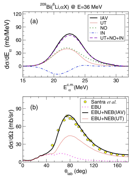
Figure 13: (Color on line) Panel (a): the IAV, UT, HM and IN cross sections; Panel (b): The inclusive BU cross sections predicted by the IAV and UT models, in comparison with data Ref. Santra et al. (2011). See the text for details.

On the other hand, more recently, Lei and Moro Lei and Moro (2015b) studied the accuracy of the IAV and the UT models, performing calculations of the ${}^{209}{\rm Bi}(^{6}{\rm Li},\alpha X)$ reaction at $E=36$ MeV. They obtained the EBU cross section by a CDCC calculation and evaluated the NBU cross section using both the UT and the IAV models. The IAV, UT, HM (denoted by NO) and the interference (IN) cross sections of Eq. (140) are shown in panel (a) of Fig. 13. The sum of the UT, HM and IN terms is represented by the long-dashed line. Note that this curve is very close to the one representing the IAV cross section, as predicted by Eq. (140).

Summing the NBE cross section of the IAV and UT models with the EBU cross section, Lei and Moro obtained the inclusive breakup cross section predicted by the two models. The results are shown in panel (b) of Fig. 13, in comparison with the data of Santra et al. Santra et al. (2011). Whereas the predictions of the IAV model reproduces very well the experimental cross section, the results of the UT model fall well below the data.

4.2 Applications

The surrogate method allows evaluation of cross sections that cannot be directly measured, such as neutron capture by short-lived targets. In this section we illustrate the use of the SM in two examples.

Neutron capture by short-lived targets

Neutron capture reactions are of great interest in nuclear physics, astrophysics and in theoretical models for generation of energy. In different situations, the direct measurement of these cross sections are very difficult to perform. One example is radioactive capture of neutrons by a short-lived target (more details on this topic can be found in Ref. Potel et al. (2017)). We will discuss below the indirect measurement of the $(n,\gamma)$ cross section for the short-lived ${}^{87}{\rm Y}$ nucleus ($t_{\rm\scriptscriptstyle 1/2}=79.8$ h), for which there are no data available. According to the Hauser-Feshbach theory Hauser and Feshbach (1952), this cross section can be written as,

$$\sigma_{n\gamma}(E_{n})=\sum_{J,\pi}\sigma_{\rm\scriptscriptstyle CN}\left(E_{\rm ex},J^{\pi}\right)\ G_{\gamma}\left(E_{\rm ex},J^{\pi}\right),$$ (142)

where $\sigma_{\rm\scriptscriptstyle CN}\left(E_{\rm ex},J^{\pi}\right)$ is the formation probability of the ${}^{88}{\rm Y}^{*}$ compound nucleus with excitation energy $E_{\rm ex}$, angular momentum $J$ and parity $\pi$, and $G_{\gamma}\left(E_{\rm ex},J^{\pi}\right)$ is the probability that the CN decays emitting one or more $\gamma$-rays. The excitation energy is related to the energy of the incident neutron by the equation, $E_{n}=(1+1/A)(E_{\rm ex}-S_{n})$, where $S_{n}$ is the energy needed to remove the neutron from ⁸⁸Y. The CN formation probability can be obtained theoretically, using a properly chosen neutron-nucleus complex potential in a standard potential scattering calculation. The decay probability $G_{\gamma}$, which is very hard to calculate, can be obtained by the surrogate method from the ${}^{89}{\rm Y}\,(p,d)\,^{88}{\rm Y}^{*}$ reaction Escher et al. (2018), through coincidence measurements of the deuteron with the characteristic $\gamma$-rays emitted by ${}^{88}{\rm Y}^{*}$. The coincidence probability can be written as,

$$P(E_{\rm ex},\theta_{d})=\sum_{J,\pi}F_{\rm\scriptscriptstyle CN}\left(E_{\rm ex},J^{\pi},\theta_{d}\right)\ G_{\gamma}\left(E_{\rm ex},J^{\pi}\right),$$ (143)

where $F_{\rm\scriptscriptstyle CN}\left(E_{\rm ex},J^{\pi},\theta_{d}\right)$ is the formation probability of a ${}^{88}{\rm Y}$ CN with quantum numbers $\{E_{\rm ex},J^{\pi}\}$ in the $(p,d)$ reaction, with the $d$ being emitted at an angle $\theta_{d}$, and $G_{\gamma}\left(E_{\rm ex},J^{\pi}\right)$ is the $\gamma$-decay probability that appears in Eq. (142). The former can be evaluated by standard nuclear reaction techniques. Then, $G_{\gamma}\left(E_{\rm ex},J^{\pi}\right)$ is expressed in terms of parameters, which were determined by fitting the experimentally determined $P(E_{\rm ex},\theta_{d})$ probability. The cross section $\sigma_{n\gamma}(E_{n})$ was then determined by inserting the resulting decay probability into Eq. (142) and using the calculated CN formation probability. The results are shown in Fig. 14, together with the TENDL 2015 (brown curves, with hatched 1 $\sigma$ uncertainty) and the Rosfond 2010 evaluations which are based on regional systematics (Nikolaev nnd (2018), Koning Koning (2015)).

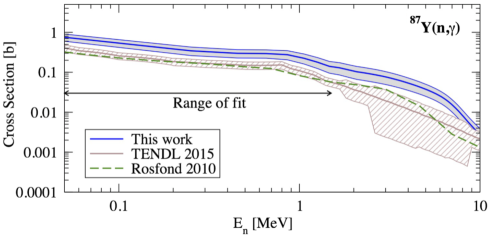
Figure 14: (Color on line) The $\sigma_{n\gamma}(E_{n})$ cross section in the $p\,+\,^{89}{\rm Y}\rightarrow d\,+\,^{88}{\rm Y}^{*}$ reaction, obtained by the SM (blue solid curve), with 1 $\sigma$ uncertainty (gray band). The figure was taken from Ref. Escher et al. (2018). For details see the text.

The validity of the SM could not be checked in the above discussed reaction because there is no direct measurement of $\sigma_{n\gamma}(E_{n})$. However, Escher et al. Escher et al. (2018) assessed the accuracy of their surrogate approach using it for another target in the same Zr-Y region. They evaluated the ${}^{90}{\rm Zr}(n,\gamma)$ cross section through the surrogate reaction ${}^{92}{\rm Zr}\,(p,d)\,^{91}{\rm Zr}^{*}$. The agreement was reasonable. The surrogate cross section and the one measured directly exhibited similar energy dependences and the same order of magnitude.

Complete fusion in collisions of weakly bound nuclei

Determining complete fusion (CF) and incomplete fusion (ICF) cross sections in collisions of weakly bound nuclei is a great challenge both for experimentalists and theoreticians Canto et al. (2015a, 2006); Jha et al. (2020). Owing to the influence of the breakup channel, the CF cross section is reduced in comparison to predictions of barrier penetration models. In the ^6,7Li + ²⁰⁹Bi and ⁹Be + ²⁰⁸Pb collisions, for example, the reduction is $\sim 20-35$ %. Recently, Lei and Moro evaluated the CF cross section using the inclusive breakup model Lei and Moro (2019). For this purpose, they wrote the total reaction cross section as,

$$\sigma_{\rm\scriptscriptstyle R}=\sigma_{\rm inel}+\sigma_{\rm\scriptscriptstyle EBU}+\sigma_{\rm\scriptscriptstyle NEB}^{\rm\scriptscriptstyle(b)}+\sigma_{\rm\scriptscriptstyle NEB}^{\rm\scriptscriptstyle(x)}+\sigma_{\rm\scriptscriptstyle CF},$$ (144)

where $\sigma_{\rm\scriptscriptstyle R},\sigma_{\rm inel},\sigma_{\rm\scriptscriptstyle EBU},\sigma_{\rm\scriptscriptstyle NEB}^{\rm\scriptscriptstyle(b)},\sigma_{\rm\scriptscriptstyle NEB}^{\rm\scriptscriptstyle(x)}$ and $\sigma_{\rm\scriptscriptstyle CF}$ are respectively the total reaction, inelastic scattering, elastic breakup, nonelastic breakup of fragments (b) and (x), and complete fusion cross sections. These cross sections were determined as follows. The $\sigma_{\rm\scriptscriptstyle R}$, $\sigma_{\rm\scriptscriptstyle EBU}$ and $\sigma_{\rm inel}$ cross sections were obtained from standard theoretical approaches (CC or CDCC calculations), and $\sigma_{\rm\scriptscriptstyle NEB}^{\rm\scriptscriptstyle(b,x)}$ were obtained from inclusive breakup model calculations as described in section 4.1. The remaining cross section, $\sigma_{\rm\scriptscriptstyle CF}$ was extracted from Eq. (144).

The method described above was used to study CF in the ^6,7Li + ²⁰⁹Bi collisions and the theoretical cross sections were compared with the data of Dasgupta et. al Dasgupta et al. (2002, 1999, 2004). The comparison is reproduced in Fig. 15.

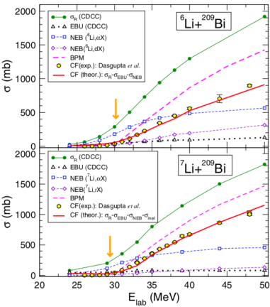
Figure 15: (Color on line) The cross sections of Eq. (144) together with the fusion cross section of barrier penetration models and the CF data. The figure was taken from Ref. Lei and Moro (2019) and the data are from Refs. Dasgupta et al. (2002, 2004).

Clearly, the surrogate approach of Lei and Moro Lei and Moro (2019) can describe the CF cross section very well, at leat for collision energies above the Coulomb barrier. On the other hand, it is unable to predict ICF cross section individually. This cross section is included in the NBE cross section, together with that for target excitations.

5 The total reaction cross section data

The total reaction cross section, $\sigma_{\rm\scriptscriptstyle R}$, is a very important quantity in collisions of heavy nuclei, since it contains information about the size of the collision partners and on the open channels. Although very desirable, determining $\sigma_{\rm\scriptscriptstyle R}$ as the sum of individual measurement of each channel is a great challenge for experimentalists. Thus, most of the available total reaction data have been obtained from optical model analyses of experimental angular distributions in elastic scattering. In this way, the angular momentum components of the nuclear S-matrix are determined, and the total reaction cross section is evaluated.

In the past two decades or so, with the development and modernization of experimental techniques, several new experiments have been performed with the purpose of determining total reaction cross sections, and investigating the reaction mechanisms involved in heavy nuclei collisions. In particular, the possibility of using radioactive beams out of short-lived nuclei has offered unique opportunities for research in the frontier field of nuclear physics. Several experiments with radioactive nuclei as projectiles have been performed, and previous reviews on these measurements can be found in Refs. Kolata et al. (2016a); Canto et al. (2015a); Keeley et al. (2009). The results of the analysis of these experiments have provided very interesting information, improving our understanding of the interaction mechanism between heavy nuclei and their structures. The strong synergy between reaction mechanism and structure of the nuclei involved in the collision allows for both static and dynamics effects to be investigated in the experiments related to the elastic scattering and direct measurements. It is important to mention that, from its beginning, nuclear physics is a science impelled by experiments. The development of nuclear physics is strongly dependent on the continuous advance of experimental techniques and instrumentation. A review on the thousands of interesting experiments related to elastic scattering and total reaction cross section would be unpractical. Thus, in this section, we are going to review and discuss some basic features of these experiments with a focus on reactions with projectile in the mass range o $6<A<20$ on medium to heavy mass target, and at energies close and above the Coulomb barrier, performed in the last 10 years or so. Special attention will be given to experiments with radioactive ion beams.

5.1 Elastic scattering measurements and total reaction cross section

As mentioned, total reaction cross sections can be obtained from optical model analyses of elastic angular distributions. Elastic scattering is the simplest process which can occur in collisions of two nuclei, since it involves only a few degrees of freedom. At low energy, the cross sections are quite large and a phenomenological approach, in which the interaction between the colliding nuclei is represented by an appropriate optical-model potential, is still a very reliable and practical method to analyze angular distribution data. Complex potentials are used to fit the experimental angular distribution and with these potentials the total reaction cross section can be determined. Investigations of elastic scattering is a very fruitful area and thousands of experiments have been carried out with very interesting results. In the past, most of the experiments were related to reactions with different combinations of complex projectile-target nuclear systems where the projectiles were stable nuclei. Elastic scattering cross sections of a quite large number of heavy-ion systems have been measured at several energies and the optical model has been found to be successful in extracting total reaction cross sections, as well as interaction radii. A large amount of nuclear reaction data can be found in the EXFOR database EXF (2020). A compilation of elastic scattering data can also be found in the webpage of the NRV project Karpov et al. (2017); Zagrebaev et al. (1999).

The important requirement in experiments related to elastic scattering is the identification and separation of the scattered particles from the large number of reaction products which can be produced in collisions between two heavy nuclei. Although it might seem to be a simple requirement, it can be more challenging for experiments with radioactive ion beam, which, sometimes, is produced as a cocktail of beams. To fulfil this requirement, a detection system with good energy, mass, and charge resolution, as well as a large dynamic range, is necessary. Over these several years of elastic scattering measurements, different experimental techniques have been developed to meet these requirements, all of which have its advantages and disadvantages. In the earlier times, the experiments with stable nuclei as projectiles, had a quite simple setup, which consisted of just a combination of thin and thick standard planar Silicon (Si) surface-barrier detectors, forming $\Delta E-E$ telescopes. This kind of detectors was largely used in experiments and they were enough for particle identification and to cover the complete angular range for precise angular distribution measurements. A recent paper discussing improvements on particle identification when using this kind of detector configuration can be found in Ref. Scarduelli et al. (2020). Although the planar silicon detectors are still being used, the recent generation of silicon detectors, with a more complex configuration, as double-sided silicon strip detectors (DSSSD), as well as gas ionizing detectors and active targets, have been developed and are being used.

The possibility of using radioactive beams out of short-lived nuclei has offered unique opportunities for research in the frontier field of nuclear physics. Many laboratories have installed or upgraded their facilities, and/or developed new techniques to produce radioactive nuclear beams. The idea of these facilities is to investigate nuclei at extreme conditions in terms of density, temperature, angular momentum and isospin. Reactions induced by these beams have been performed and exotic nuclear structures, such as halo properties, have been investigated Kolata et al. (2016a). Several laboratories are pushing to produce all kinds of exotic and very energetic species of nuclei as beams. Some laboratories use fragmentation reactions and in-flight technique to produce radioactive ion beams at intermediate energies: NSCL at MSU (USA)  NSC , RIBLL at HIRFL (China)  Sun et al. (2003), FAIR at GSI (Germany) FAI , RIBF at RIKEN (Japan) Yano (2007), LISE at GANIL (France) Anne et al. (1987), EXOTIC at INFN-LNL (Italy) Parascandolo et al. (2017), MARS at Texas A&M (USA) Tribble et al. (1989), and ACCULINNA at Dubna (Russia) Ter-Akopian et al. (2004). Other laboratories are using the ISOL technique: SPIRAL2 at GANIL (France) GAN , SPES at INFN-LNL (Italy) Bisoffi et al. (2016), REX-ISOLDE at CERN (Switzerland) Voulot et al. (2008) and ISAC at TRIUMF (Canada) TRI . There are also several laboratories producing radioactive nuclei at the lower energy regime such as Twinsol at University of Notre Dame (USA) Becchetti et al. (2003), RIBRAS (Brazil) Lichtenthäler et al. (2005), ATLAS and CARIBU at ANL (USA) Harss et al. (1999), CRIB-RIKEN (Japan) Yanagisawa et al. (2005) and SOLEROO (Australia) Rafiei et al. (2011). These laboratories are constantly improving their capabilities in terms of beam intensity, and development of new devices to increase the detection efficiency. Reviews on these facilities can be found in Refs. Blumenfeld et al. (2013) and Raabe (2016). Some new laboratories, such as VECC-RIB (India) Chakrabarti (2007), BRIF Zhang et al. (2013) and HIAF (China) Yang et al. (2013), which are under construction, will broaden even further the scope of the studies on nuclear reactions.

Most of these laboratories have scientific programs based on measurements of nuclear reactions, and several elastic scattering experiments, at energies close and above the Coulomb barrier, have been performed. These measurements allowed the extraction of total reaction cross sections and to investigate the influence of other mechanisms in the elastic scattering. The basic idea of these experiments is to obtain angular distributions for a wide range of angles and energies and extract the total reaction cross section. The angular distributions for elastic scattering can exhibit different features depending on the incident energy and on the structure of the colliding nuclei. For instance, angular distributions for tightly bound projectiles at near-barrier energies divided by the corresponding Rutherford cross section exhibit typical Fresnel oscillatory diffraction patterns Sahm et al. (1986). For light projectiles, and at higher energies, the Coulomb force is weaker and the diffractive pattern changes from Fresnel to Fraunhofer oscillations.

On the other hand, angular distributions for weakly bound nuclei may deviate from the diffractive patterns. When the binding energy of the projectile fragments is very low, their motion decouples as they approach the target, leading to nonelastic processes. Owing to the long ranges of the Coulomb and nuclear couplings, this can occur even in distant collisions, giving rise to strong absorption at forward angles. As a result, the diffractive oscillations and the Fresnel peak are damped, or completely disappear.

Some weakly-bound nuclei are called exotic, as they can exhibit peculiar properties such as halo and borromean configurations, where the valence nucleon(s) orbits around a compact core, forming an extended matter distribution Tanihata et al. (1985, 2013). Typical examples of exotic nuclei with two valence nucleons (borromean) are ⁶He, and ¹¹Li, and with one valence nucleon (halo nuclei) are ⁸B, ¹¹Be and ¹⁵C. In collisions of these nuclei with medium to heavy mass target, the breakup process is favoured during the interaction, due to the Coulomb field of the target and/or possibly a long-range component of the nuclear potential. During the collision, the charged core is decelerated by the repulsive Coulomb forces, while the valence neutrons are not affected. This phenomenon is called electric dipole polarization or Coulomb dipole excitation (CDE).

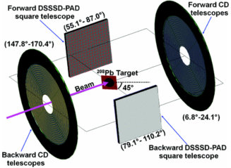
Figure 16: (Color online) Detector setup (DINEX) used in the experiment for the ⁶He+²⁰⁸Pb Acosta et al. (2011b). Figure extracted from ref. Acosta et al. (2011b).

Radioactive ion beams produced as secondary beams have the limitation of much lower intensity (in the order of $10^{3}$ up to $10^{6}$ pps), when compared to beams of stable nuclei ($\sim 10^{12}$ pps). For experiments with these beams, larger solid angles and better detection efficiency of the setup are required to compensate for the low beam intensity. State-of-art experiments, using a combination of double-sided silicon strip detectors (DSSSD) have been performed for the ⁶He, ⁸He and ¹¹Li nuclei on ²⁰⁸Pb targets. Experiments with ⁶He beams were performed at Louvain-la-Neuve (Belgium), before the facility was decommissioned, using an array of DSSSD telescopes called DINEX Acosta et al. (2011b). For the ⁸He beam, an experiment was performed at GANIL, France, using an arrangement called GLORIA (Global Reaction Array) detection system Marquínez-Durán et al. (2014, 2016), while for the ¹¹Li beam an experiment at the ISAC-II line at TRIUMF, Canada, using an array of four DSSSD telescopes, was performed Cubero et al. (2012). A sketch of the DINEX setup used in the elastic scattering of the ${}^{6}{\rm He}\,+\,^{208}{\rm Pb}$ system is shown in Fig. 16. With this kind of arrangement, a quite large total solid angle (about 20% of 4$\pi$) can be reached and a wide angular range (10^∘ to 150^∘) can be covered, allowing precise angular distribution measurements. It is also important to mention that these experiments, using low-intensity radioactive ion beams, are quite challenging from the experimental point of view. For instance, the use of detection setups with several DSSSDs demands a considerable effort in the analysis to assign the scattering and solid angles of each pixel of the array. However, all the efforts paid off, since covering a wide angular range and obtaining cross sections at very backward angles, is quite important for a better theoretical analysis and better interpretation of the influence of the several mechanisms such as breakup and transfer in the elastic scattering. The measured angular distributions obtained from these experiments have been analyzed with different approaches, such as optical model, coupled channel calculations and phenomenological models Keeley et al. (2019); Marquínez-Durán et al. (2017); So et al. (2014); Guimarães et al. (2018). From the optical model analysis reported in Ref. Keeley et al. (2019), the derived total reaction cross section for the ⁶He+²⁰⁸Pb and ⁸He+²⁰⁸Pb systems are very similar. The decoupling of the single-particle motion of the halo with respect to the core has also motivated the application of new reactions models such as the CDCC, discussed in section 3.2. In particular, the analysis performed for the ${}^{6}{\rm He}\,+\,^{208}{\rm Pb}$ data is a good example of the success of 4b-CDCC applications, as discussed in section 3.2.

Besides the previously discussed experiments with the neutron-rich borromean beams, several experiment have been performed with ¹¹Be Di Pietro et al. (2012); Acosta et al. (2009); Pesudo et al. (2017); Mazzocco et al. (2006) and ¹²B beams. ¹¹Be is a typical one-neutron halo nucleus, where the valence neutron moves around the ¹⁰Be core in an s-orbit, with the low separation energy ($S_{n}$=0.503 MeV). Differently from the borromean nuclei, ¹¹Be has the peculiarity of having one bound excited state, with excitation energy 320 keV ($j^{\pi}=1/2^{Ã}\textcent ˆ’$).

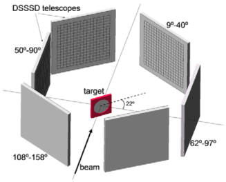
Figure 17: (Color online) T-Rex experimental setup used for the ¹⁰Be, ¹¹Be+⁶⁴Zn and ¹¹Be+¹²⁰Sn experiments at REX-ISOLDE, at CERN. Figure extracted from Ref. Acosta et al. (2009).

Di Pietro et al. Di Pietro et al. (2012) obtained high quality quasi-elastic scattering angular distribution data for collisions of ¹¹Be with ⁶⁴Zn, at energies around the Coulomb barrier. The experiment was performed at the REX-ISOLDE facility of CERN, using the array of six DSSSDs telescopes, shown in Fig. 17. Since the energy resolution was not good enough to distinguish between elastic scattering and inelastic scattering to the excited state of ¹¹Be, the angular distributions were considered quasi-elastic in nature. They also measured breakup cross sections but, due to low statistics at the backward angles, they considered only data from the three DSSSDs telescopes. The data clearly indicates the suppression of the Coulomb$-$nuclear interference peaks due to the halo structure of the ¹¹Be nucleus, which is an indication of strong absorption, even at forward angles. Indeed, the obtained total reaction cross section was $\sigma_{\rm\scriptscriptstyle R}=2730$ mb for ¹¹Be, which is more than twice those obtained for ¹⁰Be ($\sigma_{\rm\scriptscriptstyle R}=1.260$mb) and ⁹Be ($\sigma_{\rm\scriptscriptstyle R}=1.090$ mb).

Another quasi-elastic scattering experiment at the REX-ISOLDE facility was performed by Acosta et al. Acosta et al. (2009). They studied the ¹¹Be+¹²⁰Sn system, using the same setup as in the experiment of Di Pietro et al. Di Pietro et al. (2012), for the ${}^{11}{\rm Be}\,+\,^{64}{\rm Zn}$ system. Despite their impressive detection system, allowing measurements of 1536 pixels and covering an angular range of 10^∘ to 150^∘, they could only obtain reliable data at forward angles, between 15^∘ and 38^∘. This was mainly due to the use of a too thick target, which made it impossible to separate ¹¹Be from ¹⁰Be contamination at more backward angles.

Mazzoco et al. Mazzocco et al. (2007) measured elastic cross sections in collisions of ¹¹Be projectiles on a ²⁰⁹Bi target, at near-barrier energies. The experiment was performed at RIKEN, using eight two-stage $\Delta E-E$ telescopes placed along the lateral faces of two cubes closely-packed around the target, called EXODET array Mazzocco et al. (2007). Despite the large fluctuations in the cross sections, the results of the optical model analysis indicate that direct processes related to the ¹¹Be halo structure and smaller binding energies are more important at near-barrier energies.

More recently, Pesudo et al. Pesudo et al. (2017) measured elastic, inelastic and breakup angular distributions for the ${}^{11}{\rm Be}\,+\,^{197}{\rm Au}$ system. The experiment was performed at TRIUMF, Canada, with an array of 4 DSSSD telescopes surrounded by twelve high-purity germanium clovers of TIGRESS. This setup allowed measurements of elastic and inelastic scattering events at angles ranging from $14^{\circ}\,{\rm to}157^{\circ}$. The inelastic channel was identified by gating the ¹¹Be events on the 320 keV gamma-ray peak. The data were analyzed with an extended continuum-discretized coupled-channels (XCDCC), discussed in section 3.2, where the ¹⁰Be core excitation was considered. Theory and experiment were shown to be in excellent agreement (see Figs. 8 and 9).

Experiments on elastic scattering induced by proton-rich nuclei, such as ⁷Be, ⁸B, ⁹C, ¹⁰C and ¹⁷F, on medium to heavy target, have also been performed in several laboratories, as described below. One of the first experiment with ⁷Be and ⁸B secondary beams on medium to heavy target was performed at the University of Notre Dame, USA Aguilera et al. (2009b). In this experiment, angular distributions for the elastic scattering of the ⁷Be, ⁸B + ⁵⁸Ni systems were measured simultaneously, at several energies near and above the coulomb barrier. The large derived total reaction cross sections for ⁸B were considered an evidence of the halo effect in this nucleus. The CDCC calculations performed for the ⁸B + ⁵⁸Ni system showed the strong influence of the breakup channel in the elastic scattering Lubian et al. (2010); Keeley (2012).

For heavier targets, the breakup is expected to be more prominent, since the long-range Coulomb interaction is predominant over the nuclear potential. Elastic scattering measurements for the ${}^{8}{\rm B}\,+\,^{208}{\rm Pb}$ system were performed at $E_{\rm\scriptscriptstyle Lab}=50$ MeV Mazzocco et al. (2019) and $E_{\rm\scriptscriptstyle Lab}=170$ MeV Yang et al. (2018). The measurement at the lower energy, close to the barrier, was performed at the CRIB facility in RIKEN, Japan, using the EXPADES detector array Pierroutsakou et al. (2016), which consisted of six DSSSD telescopes covering the angular range of 8^∘ to 166^∘. The obtained angular distribution shows a quite strong damping of the Fresnel peak, although the differential cross sections data in the corresponding angular region show large fluctuations and uncertainties. The extracted total reaction cross section from an optical model analysis was $\sigma_{\rm\scriptscriptstyle R}=1112$ mb, which is much larger than the one for the ⁷Be core on the same target, measured in the same experiment ($\sigma_{\rm\scriptscriptstyle R}=253$ mb). Full CDCC calculations performed for the ${}^{8}{\rm B}\,+\,^{208}{\rm Pb}$ system poorly reproduces the experimental angular distribution, indicating that some other effect, such as core excitation, may be playing an important role for this system. For the data obtained at the higher energy, three times that of the Coulomb barrier, at the Radioactive Ion Beam Line in Lanzhou (RIBLL), the Fresnel peak is still present and the full CDCC calculation describes quite well the data Yang et al. (2018).

Besides the data on the ${}^{8}{\rm B}\,+\,^{58}{\rm Ni}$ system reported in Ref. Aguilera et al. (2009c), elastic scattering experiments involving other boron isotopes have been performed, studying the ${}^{10}{\rm B}\,+\,^{58}{\rm Ni}$ Scarduelli et al. (2017), ${}^{11}{\rm B}\,+\,^{58}{\rm Ni}$ Deshmukh et al. (2015) and ${}^{12}{\rm B}\,+\,^{58}{\rm Ni}$ Zevallos et al. (2019) systems. All these data were analyzed with coupled channel calculations, and the analyses indicated that the elastic cross sections are sensitive to the cluster configuration of the projectiles. Different configurations of the boron isotopes were shown to produce different effects on the elastic angular distributions Guimarães et al. (2020).

Elastic scattering experiments on collisions of ⁹C, ¹⁰C, ¹¹C, ¹²C, ¹³C, ¹⁴C, and ¹⁵C beams on heavy targets have also been performed, as described below. Santra et al. Santra et al. (2001) studied the ¹²C+²⁰⁸Pb system, measuring elastic and inelastic scattering, transfer, fission, and evaporation residue cross sections, at energies around and above the Coulomb barrier, in the range: $E_{\rm\scriptscriptstyle Lab}=58.9-84.9$ MeV. Simultaneous coupled reaction channel (CRC) calculations involving the elastic and all the nonelastic channels were performed. Optical-model analyses of the elastic data have been also carried out. The resulting optical potential showed a strong energy dependence, mainly at near-barrier energies, and some long-range absorption. Although elastic scattering and various nonelastic channels are studied in Ref. Santra et al. (2001), the total reaction cross section has not been given in this work.

Several measurements of elastic cross sections in collisions of ¹³C and ¹⁴C on heavy targets have been performed (see, for instance, the database in the website given in Ref. Karpov et al. (2017); Zagrebaev et al. (1999)). Most of these experiments investigated the influence of one- or two-neutron transfer reactions on the elastic process. In particular, the study of Landowne and Wolter for the ¹³C+²⁰⁸Pb system Landowne and Wolter (1981) at sub-barrier energies is one of the pioneering works in the early days on the use of single-folding potential models and on the importance of valence nucleon in elastic scattering.

Experiments with secondary beams of radioactive carbon isotopes have also been performed. Yang et al.Yang et al. (2018, 2014) measured elastic angular distributions for collisions of ^9,10,11C on ²⁰⁸Pb. The experiments were performed at the RIBLL in Lanzhou, China, at collision energies three times the height of the Coulomb barrier. The measured angular distributions did not show any suppression of the Fresnel peak, resembling those for stable projectile. On other hand, a strong absorption has been observed for the elastic scattering of ¹⁰C+⁵⁸Ni system at energies closer to the barrier, most probability due to the combination of deformation and cluster configuration Guimarães et al. (2019). The ¹⁰C isotope is assumed to be the only nucleus to have a brunnian (super-borromean) structure, where the four interconnected rings are associated to the four-body interactions ($\alpha+\alpha+p+p$) Curtis et al. (2008); Charity et al. (2009).

An interesting experiment was performed with the ATLAS accelerator, at ANL, to measure fusion reactions for the ${}^{12,13,14,15}{\rm C}\,+\,^{232}{\rm Th}$ systems, at near-barrier energies Alcorta et al. (2011). The ¹⁵C nucleus is a good candidate for an exotic halo nucleus. The valence neutron is orbiting around the ¹⁴C core, in an $s_{1/2}$ orbit with a binding energy of S_n=1.218 MeV. The experiment showed that, at the lowest energies, the fusion-fission cross sections for ¹⁵C+²³²Th is enhanced by a factor of 5, in comparison to those for ^12,13,14C projectiles. Considering that, at this very low energy, the fusion-fission would exhaust the total reaction cross section, this is an indication of large total reaction cross section, typical of an exotic nucleus.

Very recently an elastic scattering experiment for the ¹⁵C+²⁰⁸Pb system was performed at the HIE-ISOLDE facility, at CERN  Ovejas et al. (2020). Although they used the GLORIA detector array Marquínez-Durán et al. (2014), which covers a large solid angle and angular range of 15^∘ to 165^∘, the cross sections were determined only at the most forward angles. The preliminary data indicated a strong absorption and strong damping of the Fresnel peak.

Laboratories as GANIL (France), NSCL-MSU (USA), ANL (USA), RIKEN (Japan), TRIUMF (Canada), RIBLL (China), Dubna (Russia) etc. are producing several other radioactive ion beams, with $Z>6$, such as ¹²N, ¹³O, ¹⁴O, ¹⁷F, and ¹⁷Ne etc. However, most of the experiments are related to the investigation of the structure of these nuclei, using reactions on light targets (H and He) at high energies ($>50{\rm MeV}/A$). Very few experiments are being performed to measure reactions induced by radioactive nuclei with $Z>6$ on medium to heavy target. The exception is the ¹⁷F nucleus, where some efforts have been devoted to measure elastic scattering, breakup and fusion reaction. Fluorine-17 is a weakly-bound proton drip line nucleus, where the valence proton has the binding energy $S_{p}=0.601$ MeV. One of the first experiment involving ¹⁷F was the fusion-fission measurement of ¹⁷F+²⁰⁸Pb performed at energies in the vicinity of the Coulomb barrier at ANL, USA Harss et al. (1999). For proton drip-line nuclei, the breakup process produces a residual nucleus (the core), with one less proton, and thus with a lower Coulomb barrier. This is expected to lead to appreciable incomplete fusion, and to large total fusion cross sections. However, no enhancement of fusion-fission yields due to breakup or to a large interaction radius was observed in this experiment.

Later, some other experiments were performed Beene et al. (2011) at the Holifield Radioactive Ion Beam Facility (HRIBF) at Oak Ridge, USA, to measure elastic scattering and breakup of the same ¹⁷F+²⁰⁸Pb system Liang et al. (2002, 2003). In these works, a discussion on the diffraction and stripping breakup was presented, where the late is related to incomplete fusion of the proton fragment. Their results suggested that, for proton-rich nuclei, sub-barrier fusion would be suppressed. This is in sharp contrast with the large sub-barrier fusion enhancements observed for the exotic neutron-rich nucleus ⁶He Kolata et al. (1998a).

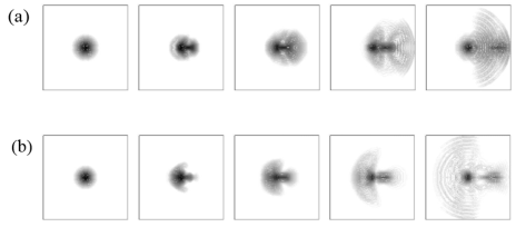
Figure 18: (Color online) Time-dependent density distribution of: (a) the neutron; (b) the proton valence particle (figure extracted from Ref. Ito et al. (2006)).

There has been some speculation about the possible polarizability of the proton- and neutron-rich exotic nuclei, as they approach a heavy target. In the case of a proton halo nucleus, both the valence proton and the core would be scattered to the backward direction by the Coulomb field of the target. On the other hand, for neutron-rich nuclei, the charged core is repelled by the Coulomb field, whereas the neutron halo is not affected. In this way, the neutron-rich projectile would be polarized along the collision. This idea is corroborated by the time-dependent dynamic calculation of the fusion process by Ito et al. Ito et al. (2006), illustrated in Fig.18. The figure shows time evolutions of the projectile’s density in a collision of a neutron-rich (panel (a)) and of a proton-rich (panel (b)) projectile with a heavy target, at a sub-barrier energy.

Due to the high interest in investigations of breakup effects in fusion, elastic and total reaction cross sections for proton-rich nuclei, other elastic scattering experiments were carried out, for the ¹⁷F+²⁰⁸Pb Signorini et al. (2010) and ¹⁷F+⁵⁸Ni Mazzocco et al. (2010) systems at near-barrier energies. The experiments were performed at INFN-LNL, Italy, using the EXOTIC facility Parascandolo et al. (2017). In these experiments the charged particles coming out from the reaction were detected by the EXODET detector array, which consisted of eight $\Delta E$-$E$ telescopes arranged as faces of two cubes closely packed in the front and at the back side of the target Romoli et al. (2005). This setup covered a solid angle of about 70% of $4\pi$ sr and allowed the coincidence detection of both ¹⁶O and $p$ fragments from the ¹⁷F breakup (exclusive breakup).

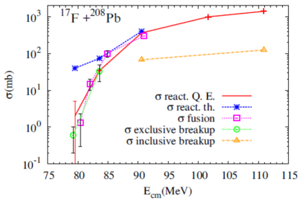
Figure 19: (Color online) Cross section for total reaction, inclusive and exclusive breakup and fusion. Figure taken from Ref. Signorini et al. (2010).

The results for the ¹⁷F+²⁰⁸Pb system are summarized in Fig. 19. At energies below the coulomb barrier (V${}_{\rm\scriptscriptstyle B}=92.0$ MeV), the sum of exclusive breakup and fusion exhausted the total reaction cross section. Above the barrier, the inclusive breakup, where only the ¹⁶O fragment is detected, was quite strong. The conclusion is that the reactivity of the proton-rich ¹⁷F nucleus is not very large. Thus, the small binding energy of the valence proton plays a minor role in the reaction dynamics.

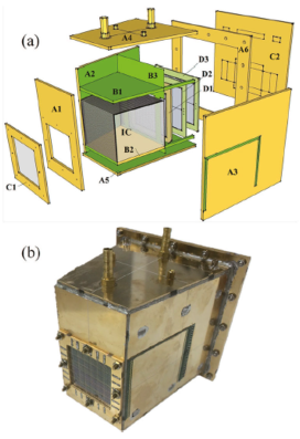
Figure 20: (Color online) View of general structure and the photograph of the assembled multilayer ionization-chamber telescope array MITA. Figure extracted from Ref. Ma et al. (2019).

Very recently, another experiment for the ¹⁷F+⁵⁸Ni system was performed at the CRIB, RIKEN, Japan. In this experiment, elastic, breakup and fusion cross sections were measured using a multilayer ionization-chamber telescope Array (MITA) Ma et al. (2019), shown in Fig. 20. This device is a combination of 10 independent telescopes, where each of them consists of four stages detectors: one ionization chamber, followed by thin (40 or 60 $\mu$m) DSSSD and two layers of thick (300 and 1000 $\mu$m) quadrant silicon detectors (QSDs). The possibility of detecting, distinguishing and separating high Z particle as well as light particles enables the simultaneous measurements of all the important reactions (elastic, breakup and fusion) produced in the collision, where the ionization chamber is important to measure energy loss of high Z particles. A single angular distribution for the elastic scattering is presented in Ref. Ma et al. (2019). The full set of data of this experiment is been submitted for publication and the results is promising and very much awaited.

Usually different experimental setups, not always available at the same laboratory, would be required to measure the different reaction channels produced in a collision between heavy nuclei. In most cases, it would demand different measurements at different times and, consequently, it would take several years to get information on all channels for a given system.

An example of such an effort is the work developed at University of Notre Dame to investigate the channels involved in the collision of ⁶He on a ²⁰⁹Bi target. The different reactions were measured in different experiments, using different setups, such as sub-fusion measurement ($1n,2n,3n$ evaporation) Kolata et al. (1998a), fusion-fission Kolata et al. (1998b), fusion-evaporation ($4n$ evaporation) DeYoung et al. (1998), transfer and breakup Aguilera et al. (2000), elastic scattering Aguilera et al. (2001), $2n$-transfer DeYoung et al. (2005) and breakup Kolata et al. (2007). The discussion of these mechanisms, in terms of total reaction cross section and evidence for core-halo decoupling, was reported in Ref. Aguilera et al. (2010). A similar effort was also devoted to the ⁸B+⁵⁸Ni system, where elastic Aguilera et al. (2009c), breakup Guimarães et al. (2000); Aguilera et al. (2008) and fusion cross sections Aguilera et al. (2011) were measured in different experiments, and with different setups. The discussion of the total reaction cross section for this system was reported in Ref. Kolata et al. (2017). The sum of the total fusion plus breakup cross sections gives about the same large total cross section as those extracted from elastic scattering, see Fig. 21.

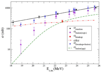
Figure 21: (Color online) The several cross sections for ⁸B+⁵⁸Ni system, as indicated. The fusion curve was calculated using the Sãão Paulo potential. Figure extracted from Ref. Kolata et al. (2017).

5.2 Direct measurements and total reaction cross section

In the previous section, some experiments on the elastic scattering of radioactive ion beams were highlighted. The total reaction cross sections were extracted from optical model (OM) analyses of the scattering data.

However, this indirect method has a limitation. It relies on a precise determination of the optical potential, which requires accurate elastic scattering data over a fine angular mesh. Frequently, this condition is not met, mainly in collisions of exotic nuclei. On the other hand, some direct methods to measure the total reaction cross section have been developed, and reported in the literature. A brief discussion of these methods is presented below.

Sum of differences

The sum of difference method, described in section 2.3, is a very convenient way to obtain the total reaction cross section and information on the nuclear interaction from the elastic angular distribution at very forward angles. In this angular region, heavy-ion scattering exhibits oscillations, known as forward glory effect. These oscillations result from the interference between the nuclear and Coulomb scattering amplitudes. As the Coulomb amplitude is known analytically, it is possible to extract $f{\rm\scriptscriptstyle N}(\theta=0)$ from the data, and then obtain the total reaction cross section (see section 2.3).

This method was used to investigate forward nuclear glory in the scattering of the ¹²C+¹²C system of identical nuclei Ostrowski et al. (1991a). Total reaction cross sections were extracted and a clear evidence of nuclear glory in heavy-ion collisions was observed. In another experiment, this method was used to study collisions of ¹²C, ¹³C, ¹⁵N and ¹⁶O projectiles on ²⁸Si targets Yamaya et al. (1998). The elastic scattering data were used to extract the total reaction cross section and to investigate the importance of the neutron transfer in the reaction.

Ueda and Takigawa studied the forward glory effect in collisions of the two-neutron halo ¹¹Li nucleus on ¹²C, within a semiclassical approximation Ueda and Takigawa (1996). They found that the halo of ¹¹Li leads to a higher glory angular momentum and shifts the first glory minimum towards a smaller angle. Further, they concluded that these features enhance the oscillations of the nuclear amplitude in the sum of difference analysis.

To investigate these effects, Ostrowski et al. Ostrowski et al. (1999) measured elastic angular distributions for the ⁶He+¹²C system at forward angles. The experiment was performed at Louvain-la-Neuve, Belgium. They concluded that the low neutron binding energy of ⁶He reduces the nuclear forward glory effect due to flux losses from the elastic channel to breakup or transfer channel, and that the total reaction cross section for this weakly bound system is twice as high at that for for ⁶Li + ¹²C at the same Coulomb parameter value.

Backscattering cross section

A simple method to extract the total reaction cross section has been proposed by Sargsyan et al. Sargsyan et al. (2013), which consists of using only the cross section measured at very backward angles.

The starting point is the usual expression for the total reaction cross section,

$$\sigma_{\rm\scriptscriptstyle R}(E)=\frac{\pi}{K^{2}}\sum_{J=0}^{\infty}\ (2J+1)\ \mathcal{P}_{\rm\scriptscriptstyle R}(J,E),$$ (145)

where $\mathcal{P}_{\rm\scriptscriptstyle R}(J,E)$ is the total reaction probability in a collision with energy $E$ and angular momentum $J$. Then, $\mathcal{P}_{\rm\scriptscriptstyle R}(0,E)$ is written in terms of the elastic scattering probability for $J=0$,

$$\mathcal{P}_{\rm\scriptscriptstyle R}(0,E)=1\,-\,\mathcal{P}_{\rm\scriptscriptstyle el}(0,E),$$ (146)

and $\mathcal{P}_{\rm\scriptscriptstyle el}(0,E)$ is approximated by the ratio between the elastic and the Rutherford cross sections at $\theta=180^{\circ}$, namely

$$\mathcal{P}_{\rm\scriptscriptstyle el}(0,E)\simeq\left[\frac{d\sigma_{\rm\scriptscriptstyle el}(\theta){\big{/}}d\Omega}{d\sigma_{\rm\scriptscriptstyle Ruth}(\theta){\big{/}}d\Omega}\right]_{\theta=180^{\circ}}.$$ (147)

Next, the total reaction probabilities for $J\neq 0$ are approximated by the probability at $J=0$, but at the lower energy

$$E^{\prime}=E\,-\,\frac{\hbar^{2}}{2\mu R_{J}^{2}}\ J(J+1),$$ (148)

where $R_{J}$ is the radius of the barrier of the effective potential (including the centrifugal term), $V_{J}(R)$.

The sum over $J$ in Eq. (145) is then transformed into an integral over $E^{\prime}$ involving $\mathcal{P}_{\rm\scriptscriptstyle R}(0,E^{\prime})$, which is related to the backscattering scattering data ($\theta_{\rm Lab}>150^{\circ}$), through Eqs. (146) and (147).

To assess the validity of the method, Sargsyan et al. Sargsyan et al. (2013) used it to evaluate cross sections for several systems: ${}^{4}{\rm He}\,+\,^{92}{\rm Mo}$, ${}^{4}{\rm He}\,+\,^{110}{\rm Cd}$, ${}^{4}{\rm He}\,+\,^{110}{\rm Cd}$, ${}^{4}{\rm He}\,+\,^{116}{\rm Cd}$, ${}^{4}{\rm He}\,+\,^{112}{\rm Sn}$, ${}^{4}{\rm He}\,+\,^{120}{\rm Sn}$, ${}^{16}{\rm O}\,+\,^{208}{\rm Pb}$ and ${}^{6,7}{\rm Li}\,+\,^{64}{\rm Zn}$. In each case, the obtained cross section was compared with total reaction data obtained by the standard method, fitting elastic angular distributions. The overall agreement was good, except for the ${}^{16}{\rm O}\,+\,^{208}{\rm Pb}$ and ${}^{6}{\rm Li}\,+\,^{64}{\rm Zn}$ systems. There was no clear justification for these discrepancies. The authors suggested that it might be related to the uncertainties in the elastic data at backward angles.

An analogous procedure can be used to determine the capture component of the total reaction cross section. In this case, one replaces in Eq. (146) the elastic cross section by the quasi-elastic one, and truncate the $J$-sum of Eq. (145) at the critical angular momentum (the limit of integration over $E^{\prime}$ is modified accordingly). Using this method, capture cross sections for the ${}^{6,7}{\rm Li}\,+\,^{64}{\rm Zn}$ systems were determined in Ref. Sargsyan et al. (2013).

Guimarães et al. Guimarães et al. (2016) performed a dedicated backscattering experiment to determine the elastic cross section for the ⁶He+²⁰⁹Bi system, at sub-barrier energies. They measured cross sections at 150^∘, with uncertainties better than 10%. Several other elastic scattering data sets for collisions of exotic beams at back angles (150^∘ or higher) are available in the literature. However, usually they have uncertainties of not less than 20%. Thus, it would be interesting to employ the backscattering method to determine the total reaction cross section for the ⁶He+²⁰⁹Bi system, using the data of Ref. Guimarães et al. (2016).

Total cross section from beam attenuation

The beam attenuation or transmission method is an old and quite simple direct method to obtain the total reaction cross section Perrin et al. (1982); Kox et al. (1984). In this method, one measures the number of particles in the incident beam, $N_{\rm\scriptscriptstyle B}$, and the number of unscattered particles plus particles scattered elastically, after the beam traverses a thick target, $N_{\rm\scriptscriptstyle T}$. The difference of the two is proportional to the total reaction cross section. That is,

$$\sigma_{\rm\scriptscriptstyle R}=k\times\ \left[\frac{N_{\rm\scriptscriptstyle B}-N_{\rm\scriptscriptstyle T}}{N_{\rm\scriptscriptstyle B}}\right],$$ (149)

where $k$ is a constant related to the target thickness. This is a reliable method to be applied to nucleus-nucleus collisions at medium to high energies (10-50 MeV/A). At first, it was used to measure the total reaction cross section in collisions of light particles ($p,d,t$ and $\alpha$) with several targets, mostly for practical applications in reactors and space science Meyer et al. (1960).

This method was first applied in an experiment performed at CERN, to measure the total reaction cross section for the ¹²C+¹²C system Perrin et al. (1982). An improvement of the method was achieved when TOF was added to the $\Delta E-E$ signals for a better identification of the particles. Details can be found in the work of Zheng et al. Zheng et al. (2013), reporting their experiment to study of the halo structure of ¹⁶C, performed at RIKEN.

Using a simular approach, Erdemshimeg et al.  Erdemchimeg et al. (2019) performed experiments at the Flerov Laboratory of Nuclear Reactions, JINR, Russia. They measured total reaction cross sections in collisions of ^4,6,8He, ^7,9,10,11,12Be, ^7,8,9Li and ^8,10,11,12B projectiles on ²⁸Si targets, at energies in the range $(10-50)\,{\rm MeV}\cdot A$. A smooth mass dependence was observed for the extracted radius, but with fluctuations for some particular projectiles. These fluctuations might be an indication of halo structure.

Another interesting experiment was performed at the Radioactive Ion Beam Line in Lanzhou (RIBLL) at the HIRFL, China. Li et al.  Jia-Xing et al. (2010) measured total reaction cross sections in collisions of the mirror nuclei ¹²N and ¹²B on ²⁸Si. The data were analyzed by Glauber model calculations, using gaussian-gaussian distributions Alkhazov et al. (2002) for the nuclear densities of ¹²N and ¹²B. The parameters of the densities were then fitted to reproduce the total reaction data. The density of ¹²N obtained in this way is consistent with the ${}^{11}{\rm C}+p$ cluster configuration.

Total reaction cross section by solid active target method

The pioneering work of Tanihata et al. Tanihata et al. (1985) on the interaction cross section in collisions of the radioactive lithium and beryllium isotopes triggered a series of experiments to measure total reaction cross sections for halo nuclei.

A simple method has been developed for this purpose, using solid active targets. In this method, the incident particles are stopped within the solid-state detector, which has the double function of detector and target. Owing to the $Q$-value of the non-reacting events ($Q=0$), it is possible to distinguish them from reacting events. The former produce a sharp peak, with large intensity, at the beam energy, $E_{0}$, whereas reactive events give much weaker contributions to the spectrum at different energies ($E=E_{0}+Q$). The energy signal in coincidence with $\gamma$-ray signals from a surrounding 4$\pi$ array of NaI(Tl) detectors can help to clean the energy spectra from spurious events, mainly in the energy region of $Q\sim 0$. The reaction probability, $\mathcal{P}_{\rm\scriptscriptstyle R}$, is then determined by dividing the number of reactive events (outside of the sharp elastic peak) by the total number of counts in this spectrum.

This method was first applied at GANIL, for silicon target-detectors and light radioactive projectiles at intermediate energies (20-50 ${\rm MeV}/A$) Villari et al. (1991). In this experiment, the mean (energy-integrated) total reaction cross section and the associated reduced radius, $r_{0}^{2}$, were obtained for several neutron-rich radioactive nuclei in the mass range $8<A<40$, such as ⁸He, ¹²Be, ¹⁵B, ²²O, ²⁶Ne, ³⁷Si. The authors observed a strong isospin-dependence in the total reaction cross section and in the reduced radius for all isobars with $A=10$ to 18.

Applying this technique and using a stack of silicon detectors, Warner et al. Warner et al. (1996, 2006) performed several experiments with proton- and neutron-rich radioactive beams at the NSCL-MSU laboratory. They performed simultaneous measurements of total reaction and multi-nucleon removal cross sections at intermediate energies. The radioactive nuclei were separated by the A1200 analyzing system of this laboratory Sherrill et al. (1992) and impinged on a stack of silicon detectors. Reaction events were then identified by the total energy loss in the telescope, which is different from that of non-reacting projectiles. Since the projectile’s energy decreases as it travels through the telescopes, the cross sections were obtained at different energies by identifying in which detector the reaction occurred. The obtained data were interpreted with the phenomenological strong absorption models and the optical limit of Glauber multiple-scattering theory. The later reproduced quite well the data.

The above technique has also been applied to low energy incident projectiles Musumarra et al. (2010). In this case, the short-range of the particles within the detector is an important issue to be considered. Besides, the reaction probability is substantially reduced by the Coulomb barrier, and this reduction leads to a low signal-to-noise ratio. Further, particles may backscatter and then leave the detector without loosing completely its energy. This would yield a small pulse that would be misinterpreted as a reaction event Warner et al. (1988). Using this technique, total reaction cross section were obtained for the ^6,7Li+²⁸Si systems at near-barrier energies Pakou et al. (2006). The measured excitation function for the total reaction cross section agrees with the data obtained in previous standard experiments, where the total reaction cross section is determined from optical model analysis of angular distributions.

The active silicon target technique has also been used to study fusion of exotic nuclei. An experiment to measure fusion cross sections for the ⁸B + ²⁸Si system was performed at LNL, Italy Pakou et al. (2013). The ⁸B secondary beam was produced at the EXOTIC facility and, from the detected evaporated alpha particles, the authors determined complete fusion cross sections at several energies above the Coulomb barrier. This measurement was based on the assumption that the observed alpha particles resulted exclusively from the evaporation of the compound nucleus formed in the collision. Their fusion excitation function was compared to data for several other weakly and tightly bound systems, measured in different experiments. To eliminate the influence of trivial factors, like charges and masses of the collision partners, the data were reduced by the fusion function method Canto et al. (2009a, b) (see section 5.3). They concluded that their reduced complete fusion cross section was similar to the data of most other systems, and to the predictions of barrier penetration models. The exception was the ⁸B+⁵⁸Ni data of Ref. Aguilera et al. (2011), obtained from the proton evaporation multiplicity. These data were much larger that those for the other systems, above and below the barrier. The ⁸B + ⁵⁸Ni and ⁸B + ²⁸Si data were later analyzed on the same basis and potentials assumptions and they were shown to be consistent with each other and in the fusion enhancement, despite the small overlap of the collision energies Aguilera et al. (2016). To clarify this issue, a new experiment was performed at the Cyclotron Institute of the Texas A&M University, USA, involving a similar system. Direct measurements of the fusion cross sections for the ${}^{8}{\rm B}\,+\,^{40}{\rm Ar}$ system were performed, using the gaseous active target TexAT Koshchiy et al. (2020) (this technique is discussed in the next section). The final results of this study are expected to be soon available.

Promising future methods

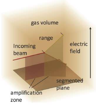
Figure 22: (Color online) Working principle of an Active target. Figure extracted from Ref. Raabe (2016).

As described in the previous sections, facilities offering radioactive ion beams are constantly improving, and developing new techniques to overcome the limitations due to the low beam intensity. One of these techniques is the use of active gaseous targets. They consist of an ionizing gas, which plays the double role of target and detector. Their geometry allows a high solid angle detection (4$\pi$), they have variable thickness, and great detection efficiency. In addition, they have good resolution, since the locations of the reaction events within the target are accurately measured.

The working principle of an active target is schematically represented in Fig. 22. The trajectory of the incident projectile (thick red line) ends at the point where the reaction takes place (red circle), giving rise to reaction products - two in this example - that follow new trajectories (thin lines). Along the trajectories, the particles ionize the medium, producing free electrons. These electrons move under the action of the vertical electric field, until they are detected on the segmented horizontal plane (bottom of the figure). In this way, the projections of the three trajectories on the horizontal ($x-y$) plane are determined. Then, three-dimensional trajectories are constructed using the information of the drift time of the pulses detected on the horizontal plane. The high luminosities achieved in gaseous active targets (due to their large dimensions in comparison with a target foil) are of great importance in experiments involving low intensity radioactive ion beams.

Active targets as the IKAR, at GSI Ilieva et al. (2012), and the MAYA, at GANIL Demonchy et al. (2007), have been used for a long time, to investigate resonant scattering and transfer reactions on hydrogen and helium targets in inverse kinematics. A review on the existing active target and its corresponding working principles can be found in Ref. Beceiro-Novo et al. (2015); Bazin et al. (2020).

A new generation of active targets, based on a time projection chamber, are becoming operational. The electrons produced by the particles inside the gaseous target drift towards a micromegas plane, which multiplies them and provide position and time information of the particle tracks. This allows a complete kinematical reconstruction of the reaction in the 3-dimensional space. The ACTAR-TPC, at GANIL Giovinazzo et al. (2020), the TexAT, at Texas A & M University Koshchiy et al. (2020), and the AT-TPC, at NSCL-MSU/University of Notre dame Mittig et al. (2015) are examples of such new generation devices. More recently, the prototype AT-TPC was used to measure fusion cross sections for the ¹⁰Be+⁴⁰Ar system Kolata et al. (2016b), indicating that this new technique can be extended to experiments with heavy targets (at least in the case of ⁴⁰Ar). This kind of device is quite promising to allow the simultaneous measurement of complete fusion, incomplete fusion, breakup, scattering, and transfer reactions, in one experiment, which is a dream for experimentalist.

Another promising experimental technique, not yet fully explored for reaction measurements, is based on the stored ion beams. The use of a heavy-ion storage ring with internal gas-jet targets, such as the ESR, at GSI Franzke (1987), or the HIRFL-CSR, at Lanzhou Xia et al. (2002), allows a great increase of the beam luminosity, since the beam revolutions in a closed trajectory with a very high frequency ($\sim 10^{6}$ MHz). However, a major challenge of this technique is to install a detector setup compatible with the ultra-high vacuum regime (in the order of 10^-10 mbar or below) needed to the operation of a storage ring. At this level any type of outgassing material can significantly deteriorate the vacuum conditions Mutterer et al. (2015). Recently, nuclear reaction experiments were successfully performed at the heavy-ion storage ring at the GSI facility, using stored ^56,58Ni beams, and hydrogen and helium internal gas-jet targets. The recoiled particles were detected by in-ring DSSSDs and angular distributions were measured, allowing studies of nuclear matter von Schmid et al. (2015); Zamora et al. (2017) and giant resonances Zamora et al. (2016). In the future this type of technique may be applied to investigate nuclear reactions using heavy jet gas targets.

5.3 Comparative studies of cross sections

It is well known that total reaction cross sections in heavy-ion collisions at near-barrier energies have important contributions from fusion and also from direct reactions (inelastic scattering, transfer, and breakup). Besides, couplings with direct reaction channels may exert a strong influence on the fusion cross section itself Beckerman et al. (1981, 1982); Reisdorf et al. (1997). An important example is the collision of a heavy or medium mass projectile with a strongly deformed target Stokstad and Gross (1981) at sub-barrier energies. The fusion cross section is several orders of magnitude larger than those for the same projectile on a spherical target with similar mass. In this way, the enhancement of the fusion cross section may be a signature of the deformation. Nevertheless, despite this enhancement, the total reaction cross section is still dominated by direct reactions in this energy region. Another example, which has attracted considerable interest in the last few decades, is the suppression of complete fusion in collisions of weakly bound nuclei (see e.g. Ref. Canto et al. (2015a) and references therein).

Clearly, comparisons of fusion and/or reaction data for different systems is a very useful tool in studies of nuclear structure and reaction mechanisms. However, direct comparisons of data for different systems may be misleading. The reason is that the cross sections also depend on trivial properties of the system, like the charges and sizes of the collision partners. We illustrate this point with an example. We consider the cross sections for collisions of ¹⁶O projectiles with energy $E_{\rm lab}=50$ MeV on two different targets: the spherical ⁴⁰Ca and the highly deformed ¹⁵⁴Sm nuclei. Estimating the cross sections by potential scattering calculations with the Akyüz-Winther potential Broglia and Winther (2004); Akyüz and Winther (1981) and short-range absorption, one finds $\sigma_{\rm\scriptscriptstyle F}=764$ mb for ⁴⁰Ca and $\sigma_{\rm\scriptscriptstyle F}=0.6\times 10^{-10}$ mb for ¹⁵⁴Sm. Clearly, the comparison of these cross sections at the same beam energy is meaningless. In the case of the ⁴⁰Ca target, the beam energy corresponds to $E_{\rm c.m.}=35.7$ MeV and the barrier is $V_{\rm\scriptscriptstyle B}=24$ MeV, whereas for ¹⁵⁴Sm the energy is $E_{\rm c.m.}=45.3$ MeV and the barrier $V_{\rm\scriptscriptstyle B}=60$ MeV. Thus, the vanishingly small cross section for the heavier target is a trivial consequence of the fact that the collision energy is almost 15 MeV below the Coulomb barrier. At this very low energy, all nonelastic cross sections are extremely low. The importance of the barrier height in comparisons of cross sections for different systems emerges more clearly in Fig. 23, which shows fusion cross sections for systems in different mass regions, as functions of the collision energy in the center of mass frame. One observes that this kind of comparison does not reveal any physical property of these systems. It only shows trivial differences in the Coulomb barriers.

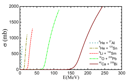
Figure 23: (Color online) Comparison of the total reaction cross sections for several systems, obtained through single-channel calculations. (Figure taken from Ref. Gomes et al. (2016)).

The examples discussed above clearly show that static properties, like the barrier height and geometric effects arising from the size of the system, must be eliminated from the analysis. For this purpose, it is necessary to make transformations on the collision energy and on the cross section to get rid of these trivial factors. This procedure is known as reduction. Several reduction methods have been proposed over the last two decades. Detailed discussions of this subject, pointing out their successes and shortcomings, can be found, e.g., in Refs. Canto et al. (2015a, b); Gomes et al. (2016). Some of the main reduction methods available in the literature are discussed below.

We begin with the traditional reduction method, which consists in the transformations,

$$E\ \rightarrow\ E_{\rm red} = \frac{E}{V_{\rm\scriptscriptstyle B}},$$ (150)

$$\sigma\ \rightarrow\ \sigma_{\rm red} = \frac{\sigma}{\pi R{\rm\scriptscriptstyle B}^{2}}.$$ (151)

Qualitatively, the above transformations go in the right direction. They modify the scales of the x- and y-axes of Fig. 23, bringing the curves of the different systems to the same region.

The second method considered here, proposed by Gomes et al. Gomes et al. (2005a), adopts the transformations,

$$E\ \rightarrow\ E_{\rm red} = E\ \times\ \left[\frac{Z_{\rm\scriptscriptstyle P}Z_{\rm\scriptscriptstyle T}}{A_{\rm\scriptscriptstyle P}^{\rm\scriptscriptstyle 1/3}+A_{\rm\scriptscriptstyle T}^{\rm\scriptscriptstyle 1/3}}\right]^{-1}$$

$$\sigma\ \rightarrow\ \sigma_{\rm red} = \frac{\sigma}{\left(A_{\rm\scriptscriptstyle P}^{\rm\scriptscriptstyle 1/3}+A_{\rm\scriptscriptstyle T}^{\rm\scriptscriptstyle 1/3}\right)^{2}}.$$ (152)

This method, inspired by the previous one, is based on the assumptions that the barrier radius scales like $A_{\rm\scriptscriptstyle P}^{\rm\scriptscriptstyle 1/3}+A_{\rm\scriptscriptstyle T}^{\rm\scriptscriptstyle 1/3}$ and that the potential barrier can be approximated by the Coulomb potential at the barrier radius. Thus, it scales like $Z_{\rm\scriptscriptstyle P}Z_{\rm\scriptscriptstyle T}/(A_{\rm\scriptscriptstyle P}^{\rm\scriptscriptstyle 1/3}+A_{\rm\scriptscriptstyle T}^{\rm\scriptscriptstyle 1/3})$. This method has the advantage of being independent of the parameters of the interaction potential, $V_{\rm\scriptscriptstyle B}$ and $R_{\rm\scriptscriptstyle B}$.

The above methods have been widely used to reduce reaction and fusion data. However, a comprehensive study of reduction methods for fusion cross sections, considering a large number of systems in different mass ranges Canto et al. (2009a, b), concluded that the best results were achieved by the fusion function method, which is discussed below.

The fusion function method hinges on the use of the Wong’s formula for the fusion cross section (Eq.(23)). The collision energy and the cross section are replaced by the dimensionless quantities Canto et al. (2009b, a),

$$E\ \rightarrow\ x=\frac{E-V_{\rm\scriptscriptstyle B}}{\hbar\omega};\ \ \ \sigma(E)\ \rightarrow\ F(x)=\frac{2\,E}{\hbar\omega\,R_{\rm\scriptscriptstyle B}^{2}}\times\sigma(E).$$ (153)

It can be immediately checked that if one applies the reduction method to the Wong’s cross section itself, one gets

$$F_{0}(x)=\ln{[1+e^{2\pi\,x}]}.$$ (154)

The above function, being basically independent on the system, is called Universal Fusion Function (UFF). The UFF would be a good representation of the reduced fusion data when they can be described by a one-channel calculations with a standard interaction, like the São Paulo Chamon et al. (1997, 2002) or the Akyüz-Winther Broglia and Winther (2004); Akyüz and Winther (1981) potential, with short-range absorption. The Wong’s formula is a reasonable approximation in heavy-ion fusion at near-barrier energies. For heavy systems ($Z_{\rm\scriptscriptstyle P}\,Z_{\rm\scriptscriptstyle P}\gtrsim 250$), it remains valid down to several MeV below $V_{\rm\scriptscriptstyle B}$. However, for lighter systems it deteriorates more rapidly as the energy decreases below $V_{\rm\scriptscriptstyle B}$. A detailed discussion of the reduction of fusion data is presented in the next section.

Reduction of fusion cross sections

The reduction of fusion cross sections by different methods has been systematically investigated in Ref. Canto et al. (2015b). The methods were submitted to a simple test. They were used to reduce theoretical cross sections obtained by one-channel calculations using the Akyüz-Winther potential and strong short-range absorption. This study involved several systems in different mass regions. Since there are no nuclear structure effects in these calculations, a successful reduction method should lead to reduced cross section with very weak system dependence. This study has shown that only the fusion function method meets this criterium. The other methods kept important system dependence, mainly in comparisons of reduced cross sections for systems in different mass ranges.

The reduction of fusion cross sections by the fusion function method is carried out in two steps, as follows.

1. The Coulomb barrier calculated with some version of the double-folding potential, like the AW or the SPP, is fitted by a parabola, and the barrier parameters $R_{\rm\scriptscriptstyle B}$, $V_{\rm\scriptscriptstyle B}$, and $\hbar\omega$ are determined.

2. The data points, $\{E_{i},\sigma(E_{i})\}$, are converted to reduced data points, $\{x_{i},F_{\rm\scriptscriptstyle exp}(x_{i})\}$, according to Eq. (153).

If there are no relevant channel coupling effects and the Wong’s formula gives an accurate description of the optical model cross section, the experimental fusion function, $F_{\rm\scriptscriptstyle exp}(x)$, is expected to be very close to the UFF. In this way, the function $F_{0}(x)$ can be used as a benchmark, to which $F_{\rm\scriptscriptstyle exp}(x)$ should be compared. Deviations from the UFF in a given energy region indicates that the Wong’s formula is inaccurate there, or it is an evidence of relevant channel coupling effects. In the latter case, the strength of the deviation measures the importance of the couplings. In most collisions, couplings with direct reaction channels play an important role in the reaction dynamics. Then, the fusion data can not be accurately described by one-channel calculations with typical heavy-ion potentials.

Usually, one wants to assess the influence of some specific process on fusion, like the breakup. Then, there may be a difficulty. The deviations of the experimental fusion function from the UFF may arise from breakup couplings and couplings with other channels. Besides, deviations may also arise from inaccuracies of the Wong’s formula. Then, the influence of such undesired effects should be minimized. This can be done introducing the renormalized experimental fusion function, denoted by $\overline{\rm F}_{\rm\scriptscriptstyle exp}(x)$, defined as,

$$F_{\rm\scriptscriptstyle exp}(x)\ \rightarrow\ \overline{\rm F}_{\rm\scriptscriptstyle exp}(x)=F_{\rm\scriptscriptstyle exp}(x)\times\frac{\sigma^{\rm\scriptscriptstyle W}(E)}{\sigma^{\rm\scriptscriptstyle CC}_{\rm\scriptscriptstyle F}(E)}.$$ (155)

Above, $\sigma^{\rm\scriptscriptstyle W}(E)$ is the Wong’s cross section of Eq. (23), and $\sigma_{\rm\scriptscriptstyle F}^{\rm\scriptscriptstyle CC}(E)$ is the theoretical fusion cross section obtained through a CC calculation that includes all relevant channels, but the ones we are investigating (usually the breakup channel). Using the reduction procedure of Eq. (155), one estimates the influence of the channels left out of the CC calculations. In Refs. Canto et al. (2009a, b), where this method was introduced, the channels left out were breakup and transfer. Of course, if all relevant channels are included in the CC calculations, the renormalized experimental fusion function is expected to coincide with the UFF. The fusion function method has been widely used in comparative studies of fusion cross sections in collisions of weakly-bound and tightly-bound projectiles Aversa et al. (2020); Kaushik et al. (2020); Torabi et al. (2020); Ali et al. (2019); Gharaei and Zhang (2019); Mazzocco et al. (2019); Rani et al. (2019); Sargsyan et al. (2017).

Detailed discussion of breakup effects on fusion

Significant channel coupling effects have been observed in collisions of weakly bound nuclei. In this case, the relevant couplings are with the breakup channel. These couplings give rise to different fusion processes. In addition to complete fusion (CF), where the whole projectile is absorbed by the target, there is incomplete fusion (ICF). The latter takes place in two steps. First, the weakly bound projectile breaks up into fragments, say two, as it interacts with the target. Then, one fragment is absorbed by the target, while to other is not. Compared with the fusion cross section of a typical one-channel calculation, the experimental CF cross section is suppressed above the Coulomb barrier, and the TF (the sum of CF and ICF) cross section is enhanced at sub-barrier energies, due to the ICF of the lighter fragment. The determination of individual CF and ICF cross sections in collisions of weakly bound projectiles is a great challenge for both experimentalists and theorists. This subject has been reviewed in several works Canto et al. (2006); Keeley et al. (2007, 2009); Canto et al. (2015a); Kolata et al. (2016a); Jha et al. (2020); Rangel et al. (2020). Most fusion experiments measure only the TF cross section. However, the available measurements of CF cross sections for weakly bound systems systematically find suppression at above-barrier energies. Further, the strongest suppressions were observed in collisions of the most weakly bound projectiles on heavy targets.

Another kind of reduction method has been used to investigate the influence of breakup couplings in the fusion of weakly bound systems. It is well established that there is suppression of a CF in collisions of weakly bound projectiles on heavy targets at above-barrier energies compared to predictions of barrier penetration models or fusion cross sections of tightly bound projectiles of similar masses. Further, the suppression is not very sensitive to the collision energy, provided that it is higher enough than the Coulomb barrier ($E_{\rm c.m.}\gtrsim V_{\rm\scriptscriptstyle B}+2\,\hbar\omega$). For comparative studies of this phenomenon, it is convenient to measure the suppression by the single number:

$${\rm F}_{\rm\scriptscriptstyle CF}=\frac{\sigma_{\rm\scriptscriptstyle CF}}{\sigma_{\rm\scriptscriptstyle TF}},$$ (156)

where $\sigma_{\rm\scriptscriptstyle CF}$ and $\sigma_{\rm\scriptscriptstyle TF}$ are respectively the complete and total fusion cross sections, above the Coulomb barrier. This procedure was used in studies ^6,7Li collisions with several medium-heavy and heavy targets, with the aim of correlating CF suppression with the mass and charge of the targets Wu et al. (2003); Rath et al. (2009); Dasgupta et al. (2002, 2004); Mukherjee et al. (2006); Kumawat et al. (2012); Pradhan et al. (2011); Shrivastava et al. (2009); Gautam et al. (2020). They concluded that F_CF has a weak target dependence. It is between 0.60 and 0.67 for ⁶Li, and between 0.70 and 0.75 for ⁷Li. It is not surprising that the largest suppressions (lowest F_CF) were found for ⁶Li, which has a lower breakup threshold.

Jha et al. Jha et al. (2014) carried out a study along the same line, for collisions of ⁹Be on several targets. They investigated the correlation of the fusion processes with the charge of the target. Instead of ${\rm F}_{\rm\scriptscriptstyle CF}$, they used an ICF probability, $P_{\rm\scriptscriptstyle ICF}$, defined as

$$P_{\rm\scriptscriptstyle ICF}=1\,-\,{\rm F}_{\rm\scriptscriptstyle CF}.$$ (157)

They concluded that the dependence of the CF/ICF processes on the target is more pronounced than that observed for the ^6,7Li projectiles.

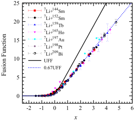
Figure 24: (Color online) Experimental fusion function for collisions of ⁴Li with different heavy targets (figure taken from Ref. Wang et al. (2014)).

A similar reduction method has been used to study the influence of the breakup threshold of the projectile on the CF cross section Wang et al. (2014); Shuaib et al. (2018). These studies considered CF data of several weakly bound projectiles on different targets, with mass numbers in the range $89\leq A_{\rm\scriptscriptstyle T}\leq 209$. They found that the experimental fusion functions were essentially independent or the target. This is illustrated in Fig. 24, which shows experimental fusion functions for collisions of ⁷Li on different heavy targets. One observes that the data points follow the dotted line, corresponding to $0.67\times F_{\rm\scriptscriptstyle 0}(x)$. Then, the authors adopt the suppression factor

$$F_{\rm\scriptscriptstyle{B.U.}}=\frac{F(x)}{F_{\rm\scriptscriptstyle 0}(x)}$$ (158)

to express the influence of the breakup channel on CF.

On the other hand, the suppression factor has an appreciable dependence on the breakup threshold of the projectile. This can be seen in Fig. 25, which shows the logarithm of $1-F_{\rm\scriptscriptstyle{B.U.}}$, as a function of the breakup threshold of the projectile, $E_{\rm\scriptscriptstyle B.U.}$.

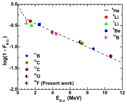
Figure 25: (Color online) Dependence of the suppression factor on the breakup threshold of the projectile. (Figure taken from Ref. Shuaib et al. (2018)).

Reduction of the reaction cross section data

The reduction of total reaction (TR) data is much more complicated because they are sums of contributions from fusion and direct reactions, which have very different natures. Fusion is absorption by a strong imaginary potential acting within the inner region of the Coulomb barrier. In this way, it is equivalent to a barrier penetration problem. For this reason, the cross section scales with the barrier parameters, as predicted by the Wong formula. This explains the success of the fusion function method to reduce fusion data. On the other hand, direct reactions are processes taking place in peripheral collisions. In 1-channel calculations, they can be simulated by a long-range imaginary potential, reaching beyond the barrier radius. These processes do not depend on the barrier parameters as predicted by the Wong formula.

Owing to the different characteristics of fusion and direct reactions, the available reduction methods have poor performances when applied to total reaction data. A detailed study of this problem was carried out in Refs. Canto et al. (2015b); Gomes et al. (2016). Different reduction methods were applied to total reaction cross sections obtained by 1-channel calculations using the Akyüz-Winther interaction Akyüz and Winther (1981); Broglia and Winther (2004), $V_{\rm\scriptscriptstyle N}(R)$, and the long-range imaginary potential, $W(R)=0.78\,V_{\rm\scriptscriptstyle N}(R)$. This procedure was applied to a large number of systems in different mass regions. Since the calculations did not take into account nuclear structure properties of the collision partners, differences among the reduced cross sections should be attributed to the gross properties of the systems, like charges and masses. Such differences should not be found in a successful reduction method. This study has shown that the reduced cross sections kept a strong system dependence, independently of the method used. Nevertheless, the situation was much better when the comparison involved systems of similar masses.

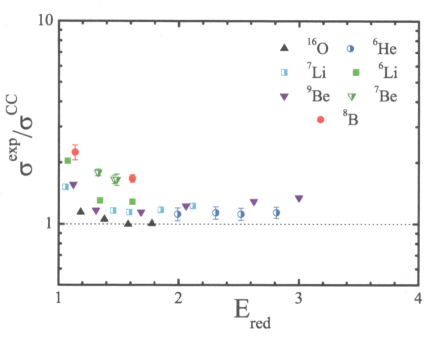
Figure 26: (Color online) Reduced TR cross sections for collisions of several projectiles on ²⁷Al, obtained by the procedure of Eq. (159) (figure taken from Ref. Morcelle et al. (2017)).

Recently, Morcelle et al. Morcelle et al. (2017) proposed a new procedure to reduce TR data, which emphasises the influence of the breakup channel. This method was applied to collisions of several weakly and tightly bound projectiles on ²⁷Al. The method consists of the transformations,

$$E\ \rightarrow\ E_{\rm{red}}=\frac{E}{V_{\rm\scriptscriptstyle B}};\ \ \ \sigma^{\rm\scriptscriptstyle{exp}}_{\rm\scriptscriptstyle{R}}\ \rightarrow\ \sigma_{\rm{red}}=\frac{\sigma^{\rm\scriptscriptstyle{exp}}_{\rm\scriptscriptstyle{R}}}{\sigma^{\rm\scriptscriptstyle{CC}}_{\rm\scriptscriptstyle{F}}},$$ (159)

where $\sigma^{\rm\scriptscriptstyle{CC}}_{\rm\scriptscriptstyle{F}}$ is the fusion cross section obtained by a CC calculation including couplings with the low-lying collective states of the ²⁷Al target, and $\sigma^{\rm\scriptscriptstyle{exp}}_{\rm\scriptscriptstyle R}$ is the total reaction cross section obtained from fits to elastic scattering data. They considered data at above barrier energies for the following systems: ⁸B + ²⁷Al Morcelle et al. (2017), ⁶He + ²⁷Al Benjamim et al. (2007), ⁶Li + ²⁷Al Figueira et al. (2007), ⁷Li + ²⁷Al Figueira et al. (2006), ⁹Be + ²⁷Al Gomes et al. (2004); Martí et al. (2005), ⁷Be + ²⁷Al Morcelle et al. (2014b), and ¹⁶O + ²⁷Al Crema (1979). Sub-barrier energies were left out because, in this energy region, the angular distribution corresponds, basically, to Rutherford scattering. In this way, the determination of the nuclear S-matrix tends to be inaccurate, leading to large error bars in the TR cross section. Breakup couplings, which hinder complete fusion, has the opposite effect on the total reaction cross section. It gives an additional contribution, which enhances TR. Therefore, $\sigma_{\rm{red}}$ must be larger than one.

The reduced cross sections obtained in Ref. Morcelle et al. (2017) are shown in Fig. 26. First, one notices that the reduced cross sections systematically increase as $E_{\rm{red}}$ decreases. This is a trivial consequence of the fact that the contribution from direct processes is dominant at low energies. Second, one observes that comparing data of different systems in the same energy range, the largest reduced cross sections are for the projectiles with the lowest breakup thresholds.

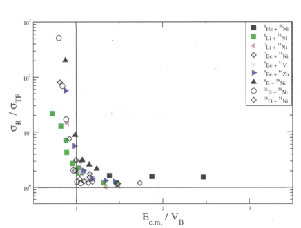
Figure 27: (Color online) Comparison of the reduced total reaction cross sections for several projectiles on medium mass range targets., obtained through coupled-channel calculations. The experimental data were taken from Ref. Morcelle et al. (2014a) for ⁶He + ⁵⁸Ni, Refs. Aguilera et al. (2009b); Biswas et al. (2008); Pfeiffer et al. (1973) for ⁶Li + ⁵⁸Ni, Ref. Pfeiffer et al. (1973) for ⁷Li + ⁵⁸Ni, Refs. Aguilera et al. (2009b); Mazzocco et al. (2015) for ⁷Be + ⁵⁸Ni, Ref. Morales-Rivera et al. (2016) for ⁹Be + ⁵¹V, Ref. Gomes et al. (2005b) for ⁹Be + ⁶⁴Zn, Ref. Aguilera et al. (2009b) for ⁸B + ⁵⁸Ni, Ref. Deshmukh et al. (2015) for ¹¹B + ⁵⁸Ni, and Ref. Keeley et al. (1995) for the ¹⁶O + ⁶⁴Zn system (Figure taken from Ref. Deshmukh and Lubian (2018)).

Deshmukh, Lubian, and Mukherjee Deshmukh et al. (2019); Deshmukh and Lubian (2018) used the same reduction procedure to investigate the TR cross sections in collisions of stable and radioactive weakly bound projectiles with intermediate mass targets, also considering data below the Coulomb barrier. Their results are shown in Fig. 27. As could be expected, the reduced cross section below $V_{\rm\scriptscriptstyle B}$ grows abruptly, reaching very high values. However, the correlation between the reduced cross section and the breakup threshold of the projectile emerges clearly, in the whole energy interval. The data points for the stable weakly bound nuclei (⁶Li, ⁷Li, and ⁹Be) are clearly above those for the tightly bound ¹⁶O, and the ones for the radioactive projectiles (⁶He, ⁸B and ¹¹Be), which have breakup thresholds below 1 MeV, are still higher.

6 Summary

We have presented an account of recent theoretical and experimental developments in the study of nuclear reactions at near-barrier energies, with emphasis on weakly bound systems and in evaluations of the total reaction cross sections. Nuclear reactions with weakly bound nuclei have large breakup cross sections, and other reaction channels are strongly influenced by the breakup process.

We began reviewing the main features of the quantum mechanical treatment of potential scattering, and its semiclassical approximations. Then, we have discussed the coupled channel approach, with emphasis in the discretization of the continuum, which is essential to describe collisions of weakly bound nuclei. The influence of core and target excitations on the elastic and reaction cross sections were then reviewed, and a few applications were considered.

We addressed also the surrogate method to describe inclusive cross sections in collisions of weakly bound nuclei. Different formulations of the method were discussed and a few examples were given.

A detailed discussion of the available methods to measure the total reaction cross section has been presented, with emphasis on the most recent experimental techniques to measure cross sections in experiments with low intensity secondary beams of unstable nuclei. We then discussed reduction method to allow meaningful comparisons of data for different systems. We pointed out that the fusion function reduction method works very well for fusion data, even for very different systems, but satisfactory reductions of total reaction data can only be achieved for very similar systems.

References

- Canto et al. (2006) L. F. Canto, P. R. S. Gomes, R. Donangelo, and M. S. Hussein, Phys. Rep. 424, 1 (2006).
- Keeley et al. (2007) N. Keeley, R. Raabe, N. Alamanos, and J. L. Sida, Prog. Part. Nucl. Phys. 59, 579 (2007).
- Keeley et al. (2009) N. Keeley, N. Alamanos, K. W. Kemper, and K. Rusek, Prog. Part. Nucl. Phys. 63, 396 (2009).
- Canto et al. (2015a) L. F. Canto, P. R. S. Gomes, R. Donangelo, J. Lubian, and M. S. Hussein, Phys. Rep. 596, 1 (2015a).
- Kolata et al. (2016a) J. J. Kolata, V. Guimarães, and E. F. Aguilera, Eur. Phys. J. A 52, 123 (2016a).
- Montagnoli and Stefanini (2017) G. Montagnoli and A. M. Stefanini, Eur. Phys. J. A 53, 169 (2017).
- Bonaccorso (2018) A. Bonaccorso, Prog. Part. Nucl. Phys. 101, 1 (2018).
- Jha et al. (2020) V. Jha, V. V. Parkar, and S. Kailas, Phys. Rep. 845, 1 (2020).
- Sakuragi et al. (1986) Y. Sakuragi, M. Yahiro, and M. Kamimura, Prog. Theoret. Phys. Suppl. 89, 136 (1986).
- Austern et al. (1987) N. Austern, Y. Iseri, M. Kamimura, M. Kawai, G. Rawitscher, and M. Yashiro, Phys. Rep. 154, 125 (1987).
- Hagino et al. (2000) K. Hagino, A. Vitturi, C. H. Dasso, and S. M. Lenzi, Phys. Rev. C 61, 037602 (2000).
- Diaz-Torres and Thompson (2002) A. Diaz-Torres and I. J. Thompson, Phys. Rev. C 65, 024606 (2002).
- Diaz-Torres et al. (2003) A. Diaz-Torres, I. J. Thompson, and C. Beck, Phys. Rev. C 68, 044607 (2003).
- Hussein et al. (1991) M. S. Hussein, R. A. Rego, and C. A. Bertulani, Phys. Rep. 201, 279 (1991).
- Chamon et al. (1997) L. C. Chamon, D. Pereira, M. S. Hussein, M. A. Candido Ribeiro, and D. Galetti, Phys. Rev. Lett. 79, 5218 (1997).
- Chamon et al. (2002) L. C. Chamon, B. V. Carlson, L. R. Gasques, D. Pereira, C. De Conti, M. A. G. Alvarez, M. S. Hussein, M. A. Cândido Ribeiro, E. S. Rossi Jr., and C. P. Silva, Phys. Rev. C 66, 014610 (2002).
- Gasques et al. (2006) L. R. Gasques, L. C. Chamon, P. R. S. Gomes, and J. Lubian, Nucl. Phys. A 764, 135 (2006).
- Broglia and Winther (2004) R. A. Broglia and A. Winther, Heavy Ion Reactions (Westview Press, 2004).
- Akyüz and Winther (1981) O. Akyüz and A. Winther, in Nuclear Structure of Heavy Ion Reaction, edited by R. A. Broglia, C. H. Dasso, and R. A. Ricci (North Holland, 1981), proc. E. Fermi Summer School of Physics.
- Canto and Hussein (2013) L. F. Canto and M. S. Hussein, Scattering Theory of Molecules, Atoms and Nuclei (World Scientific Publishing Co. Pte. Ltd., 2013).
- Feshbach et al. (1947) H. Feshbach, D. C. Peasly, and V. F. Weisskopft, Phys. Rev. 71, 145 (1947).
- Rawitscher (1964) G. H. Rawitscher, Phys. Rev. 135, B605 (1964).
- Rawitscher (1966) G. H. Rawitscher, Nucl. Phys. 85, 337 (1966).
- Kemble (1935) E. C. Kemble, Phys. Rev. 48, 549 (1935).
- Toubiana et al. (2017a) A. J. Toubiana, L. F. Canto, and M. S. Hussein, Eur. Phys. J. A 53, 34 (2017a).
- Toubiana et al. (2017b) A. J. Toubiana, L. F. Canto, and M. S. Hussein, Braz. J. Phys. 47, 321 (2017b).
- Wong (1973) C. Y. Wong, Phys. Rev. Lett. 31, 766 (1973).
- Rowley and Hagino (2015) N. Rowley and K. Hagino, Phys. Rev. C 91, 044617 (2015).
- Toubiana et al. (2017c) A. J. Toubiana, L. F. Canto, R. Donangelo, and M. S. Hussein, Phys. Rev. C 96, 064615 (2017c).
- Frahn (1966) W. E. Frahn, Nucl. Phys. A 75, 577 (1966).
- Frahn (1985) W. E. Frahn, Diffraction processes in Nuclear Physics (Oxford University Press, Oxford U.K., 1985).
- Holdeman and Thaler (1965a) J. T. Holdeman and R. M. Thaler, Phys. Rev. Lett. 14, 81 (1965a).
- Holdeman and Thaler (1965b) J. T. Holdeman and R. M. Thaler, Phys. Rev. 139, B 1186 (1965b).
- Marty (1983) C. Marty, Z. Phys. 309, 261 (1983).
- Ueda et al. (1999) M. Ueda, M. P. Pato, M. S. Hussein, and N. Takigawa, Nucl. Phys. A 648, 229 (1999).
- Barrette and Alamanos (1985a) J. Barrette and N. Alamanos, Phys. Lett. B 153, 208 (1985a).
- Barrette and Alamanos (1985b) J. Barrette and N. Alamanos, Nucl. Phys. A 441, 733 (1985b).
- Ostrowski et al. (1991a) A. N. Ostrowski, W. Tiereth, and H. Voit, Phys. Rev. C 44, 2082 (1991a).
- Shkolnik et al. (1978) V. Shkolnik, D. Dehnhard, S. Kubono, M. Franey, and S. Tripp, Phys. Lett. B 74, 195 (1978).
- Ostrowski et al. (1991b) A. N. Ostrowski, W. Thiereth, and H. Voit, Phys. Rev. C 44, 2082 (1991b).
- Ueda et al. (1998) M. Ueda, M. P. Pato, M. S. Hussein, and N. Takigawa, Phys. Rev. Lett. 81, 1809 (1998).
- Canto et al. (2009a) L. F. Canto, P. R. S. Gomes, J. Lubian, L. C. Chamon, and E. Crema, J. Phys. G: Nucl. Part. Phys. 36, 015109 (2009a).
- Canto et al. (2009b) L. F. Canto, P. R. S. Gomes, J. Lubian, L. C. Chamon, and E. Crema, Nucl. Phys. A 821, 51 (2009b).
- Canto et al. (2015b) L. F. Canto, D. R. Mendes Junior, P. R. S. Gomes, and J. Lubian, Phys. Rev. C 92, 014626 (2015b).
- Kolinger et al. (2018) G. D. Kolinger, L. F. Canto, R. Donangelo, and S. R. Souza, Phys. Rev. C 98, 044604 (2018).
- Druet et al. (2010) T. Druet, D. Baye, P. Descouvemont, and J.-M. Sparenberg, Nucl. Phys. A 845, 88 (2010).
- Thompson and Nunes (2009) I. J. Thompson and F. M. Nunes, Nuclear Reactions for Astrophysics: Principles, Calculation and Applications (Cambridge University Press, 2009), 1st ed.
- Matsumoto et al. (2003) T. Matsumoto, T. Kamizato, K. Ogata, Y. Iseri, E. Hiyama, M. Kamimura, and M. Yahiro, Phys. Rev. C 68, 064607 (2003).
- Bertulani and Canto (1992) C. A. Bertulani and L. F. Canto, Nucl. Phys. A539, 163 (1992).
- Marta et al. (2008) H. D. Marta, L. F. Canto, and R. Donangelo, Phys. Rev. C78, 034612 (2008).
- Marta et al. (2014) H. D. Marta, L. F. Canto, and R. Donangelo, Phys. Rev. C 89, 034625 (2014).
- Hiyama et al. (2003) E. Hiyama, Y. Kino, and M. Kamimura, Prog. Part. Nucl. Phys. 51, 223 (2003).
- Hesse et al. (1998) M. Hesse, J.-M. Sparenberg, F. Van Raemdonck, and D. Baye, Nucl. Phys. A 640, 37 (1998).
- Moro and Gómez-Camacho (2016) A. M. Moro and J. Gómez-Camacho, EPJ Web of Conferences 117, 06002 (2016).
- Summers et al. (2006) N. C. Summers, F. M. Nunes, and I. J. Thompson, Phys. Rev. C 74, 014606 (2006).
- Summers and Nunes (2007) N. C. Summers and F. M. Nunes, Phys. Rev. C 76, 014611 (2007).
- Moro and Crespo (2012) A. M. Moro and R. Crespo, Phys. Rev. C 85, 054613 (2012).
- de Diego et al. (2014) R. de Diego, J. M. Arias, J. A. Lay, and A. M. Moro, Phys. Rev. C 89, 064609 (2014).
- Chen et al. (2016) J. Chen, J. L. Lou, Y. L. Ye, Z. H. Li, Y. C. Ge, Q. T. Li, J. Li, W. Jiang, Y. L. Sun, H. L. Zang, et al., Phys. Rev. C 93, 034623 (2016).
- de Diego et al. (2017) R. de Diego, R. Crespo, and A. M. Moro, Phys. Rev. C 95, 044611 (2017).
- Pesudo et al. (2017) V. Pesudo, M. J. G. Borge, A. M. Moro, J. A. Lay, E. Nácher, J. Gómez-Camacho, O. Tengblad, L. Acosta, M. Alcorta, M. A. G. Alvarez, et al., Phys. Rev. Lett. 118, 152502 (2017).
- Lay et al. (2016) J. A. Lay, R. de Diego, R. Crespo, A. M. Moro, J. M. Arias, and R. C. Johnson, Phys. Rev. C 94, 021602 (2016).
- Satou et al. (2008) Y. Satou, T. Nakamura, N. Fukuda, and et al., Phys. Lett. B 660, 320 (2008).
- Lubian et al. (2009) J. Lubian, T. Correa, E. F. Aguilera, L. F. Canto, A. Gomez-Camacho, E. M. Quiroz, and P. R. S. Gomes, Phys. Rev. C 79, 064605 (2009).
- Aguilera et al. (2009a) E. F. Aguilera, E. Martinez-Quiroz, D. Lizcano, A. Gómez-Camacho, J. J. Kolata, L. O. Lamm, V. Guimarães, R. Lichtenthäler, O. Camargo, F. D. Becchetti, et al., Phys. Rev. C 79, 021601 (2009a).
- Woodward et al. (2012) A. E. Woodward, J. M. Figueira, D. R. Otomar, J. O. Fernández Niello, J. Lubian, A. Arazi, O. A. Capurro, P. Carnelli, L. Fimiani, G. V. Martí, et al., Nucl. Phys. A 873, 17 (2012).
- Gómez-Ramos and Moro (2017) M. Gómez-Ramos and A. M. Moro, Phys. Rev. C 95, 034609 (2017).