Statistical dynamics of a hard sphere gas:
fluctuating Boltzmann equation and large deviations

Résumé

We present a mathematical theory of dynamical fluctuations for the hard sphere gas in the Boltzmann-Grad limit. We prove that: (1) fluctuations of the empirical measure from the solution of the Boltzmann equation, scaled with the square root of the average number of particles, converge to a Gaussian process driven by the fluctuating Boltzmann equation, as predicted in [S81]; (2) large deviations are exponentially small in the average number of particles and are characterized, under regularity assumptions, by a large deviation functional as previously obtained in [Rez2] for dynamics with stochastic collisions. The results are valid away from thermal equilibrium, but only for short times. Our strategy is based on uniform a priori bounds on the cumulant generating function, characterizing the fine structure of the small correlations.

Chapitre 1 Introduction

This paper is devoted to a detailed analysis of the dynamical correlations arising, at low density, in a deterministic particle system obeying Newton’s laws. In this chapter we start by defining our model precisely, and recalling the fundamental result of Lanford on the short-time derivation of the Boltzmann equation, as a law of large numbers. After that, we state our main results, Theorem 2 and Theorem 3 below, regarding small fluctuations and large deviations of the empirical measure, respectively. Finally, the last part of this introduction describes the essential features of the proofs, the organization of the paper, and presents some open problems.

1 The hard-sphere model with random initial data

We consider a system of $N\geq 0$ spheres of diameter ${\varepsilon}>0$ in the $d$-dimensional torus $\mathbb{T}^{dN}$ with $d\geq 2$. The positions $({\bf x}^{{\varepsilon}}_{1},\dots,{\bf x}^{{\varepsilon}}_{N})\in\mathbb{T}^{dN}$ and velocities $({\bf v}^{{\varepsilon}}_{1},\dots,{\bf v}^{{\varepsilon}}_{N})\in\mathbb{R}^{dN}$ of the particles satisfy Newton’s laws

$${d{\bf x}^{{\varepsilon}}_{i}\over dt}={\bf v}^{{\varepsilon}}_{i}\,,\quad{d{\bf v}^{{\varepsilon}}_{i}\over dt}=0\quad\hbox{ as long as \ }|{\bf x}^{{\varepsilon}}_{i}(t)-{\bf x}^{{\varepsilon}}_{j}(t)|>{\varepsilon}\quad\hbox{for \ }1\leq i\neq j\leq N\,,$$ (1.1)

with specular reflection at collisions

$$\left.\begin{aligned} \left({\bf v}^{{\varepsilon}}_{i}\right)^{\prime}&:={\bf v}^{{\varepsilon}}_{i}-\frac{1}{{\varepsilon}^{2}}({\bf v}^{{\varepsilon}}_{i}-{\bf v}^{{\varepsilon}}_{j})\cdot({\bf x}^{{\varepsilon}}_{i}-{\bf x}^{{\varepsilon}}_{j})\,({\bf x}^{{\varepsilon}}_{i}-{\bf x}^{{\varepsilon}}_{j})\\ \left({\bf v}^{{\varepsilon}}_{j}\right)^{\prime}&:={\bf v}^{{\varepsilon}}_{j}+\frac{1}{{\varepsilon}^{2}}({\bf v}^{{\varepsilon}}_{i}-{\bf v}^{{\varepsilon}}_{j})\cdot({\bf x}^{{\varepsilon}}_{i}-{\bf x}^{{\varepsilon}}_{j})\,({\bf x}^{{\varepsilon}}_{i}-{\bf x}^{{\varepsilon}}_{j})\end{aligned}\right\}\quad\hbox{ if }|{\bf x}^{{\varepsilon}}_{i}(t)-{\bf x}^{{\varepsilon}}_{j}(t)|={\varepsilon}\,.$$ (1.2)

Observe that these boundary conditions do not cover all possible situations, as for instance triple collisions are excluded. Nevertheless the hard-sphere flow generated by (1.1)-(1.2) (free transport of $N$ spheres of diameter ${\varepsilon}$, plus instantaneous reflection

$$\big{(}{\bf v}^{{\varepsilon}}_{i},{\bf v}^{{\varepsilon}}_{j}\big{)}\to\Big{(}\big{(}{\bf v}^{{\varepsilon}}_{i}\big{)}^{\prime},\big{(}{\bf v}^{{\varepsilon}}_{j}\big{)}^{\prime}\Big{)}$$

at contact) is well defined on a full measure subset of ${\mathcal{D}}^{{\varepsilon}}_{N}$ (see [Ale75], or [GSRT] for instance) where ${\mathcal{D}}^{{\varepsilon}}_{N}$ is the canonical phase space

$${\mathcal{D}}^{{\varepsilon}}_{N}:=\big{\{}Z_{N}\in\mathbb{D}^{N}\,:\,\forall i\neq j\,,\quad|x_{i}-x_{j}|>{\varepsilon}\big{\}}\,.$$

We have denoted $Z_{N}:=(X_{N},V_{N})\in(\mathbb{T}^{d}\times\mathbb{R}^{d})^{N}$ the positions and velocities in the extended space $\mathbb{D}^{N}:=(\mathbb{T}^{d}\times\mathbb{R}^{d})^{N}$ with $X_{N}:=(x_{1},\dots,x_{N})\in\mathbb{T}^{dN}$ and $V_{N}:=(v_{1},\dots,v_{N})\in\mathbb{R}^{dN}$. We set $Z_{N}=(z_{1},\dots,z_{N})$ with $z_{i}=(x_{i},v_{i})$.

The probability density $W^{{\varepsilon}}_{N}$ of finding $N$ hard spheres of diameter ${\varepsilon}$ at configuration $Z_{N}$ at time $t$ is governed by the Liouville equation in the $2dN$-dimensional phase space

$${\partial}_{t}W^{{\varepsilon}}_{N}+V_{N}\cdot\nabla_{X_{N}}W^{{\varepsilon}}_{N}=0\,\,\,\,\,\,\,\,\,\hbox{on }\,\,\,{\mathcal{D}}^{{\varepsilon}}_{N}\,,$$ (1.3)

with specular reflection on the boundary. If we denote

$${\partial}{\mathcal{D}}^{{\varepsilon}\pm}_{N}(i,j):=\Big{\{}Z_{N}\in\mathbb{D}^{N}\,: |x_{i}-x_{j}|={\varepsilon}\,,\quad\pm(v_{i}-v_{j})\cdot(x_{i}-x_{j})>0$$

$$\mbox{and}\quad\forall(k,\ell)\in[1,N]^{2}\setminus\{i,j\},\,\,\,k\neq\ell\,,\,\,\,|x_{k}-x_{\ell}|>{\varepsilon}\Big{\}}\,,$$

then

$$\forall Z_{N}\in{\partial}{\mathcal{D}}^{{\varepsilon}+}_{N}(i,j)\,,i\neq j\,,\quad W^{{\varepsilon}}_{N}(t,Z_{N}):=W^{{\varepsilon}}_{N}(t,Z_{N}^{{}^{\prime}i,j})\,,$$ (1.4)

where $Z^{{}^{\prime}i,j}_{N}$ differs from $Z_{N}$ only by $\left(v_{i},v_{j}\right)\to\left(v^{\prime}_{i},v^{\prime}_{j}\right)$, given by (1.2).

The canonical formalism consists in fixing the number $N$ of particles, and in studying the probability density $W^{{\varepsilon}}_{N}$ of particles in the state $Z_{N}$ at time $t$, as well as its marginals. The main drawback of this formalism is that fixing the number of particles creates spurious correlations (see e.g. [EC81, PS17]). We are rather going to define a particular class of distributions on the grand canonical phase space

$${\mathcal{D}}^{\varepsilon}:=\bigcup_{N\geq 0}{\mathcal{D}}^{{\varepsilon}}_{N}\,,$$

where the number of particles is not fixed but given by a modified Poisson law (actually ${\mathcal{D}}^{{\varepsilon}}_{N}=\emptyset$ for large $N$). For notational convenience, we work with functions extended to zero over $\mathbb{D}^{N}\setminus\overline{{\mathcal{D}}^{{\varepsilon}}_{N}}$. Given a probability distribution $f^{0}:\mathbb{D}\to\mathbb{R}$ satisfying

$$|f^{0}(x,v)|+|\nabla_{x}f^{0}(x,v)|\ \leq C_{0}\,\exp\Big{(}-\frac{\beta_{0}}{2}|v|^{2}\Big{)}\,,\quad C_{0}\geq 1\,,\,\,\beta_{0}>0\,,$$ (1.5)

the initial probability density is defined on the configurations $(N,Z_{N})\in\mathbb{D}^{\mathbb{N}}$ as

$$\frac{1}{N!}W^{{\varepsilon}0}_{N}(Z_{N}):=\frac{1}{\mathcal{Z}^{\varepsilon}}\,\frac{\mu_{\varepsilon}^{N}}{N!}\,\prod_{i=1}^{N}f^{0}(z_{i})\,{\bf 1}_{{\mathcal{D}}^{{\varepsilon}}_{N}}(Z_{N})$$ (1.6)

where $\mu_{\varepsilon}>0$ and the normalization constant $\mathcal{Z}^{\varepsilon}$ is given by

$$\mathcal{Z}^{\varepsilon}:=1+\sum_{N\geq 1}\frac{\mu_{\varepsilon}^{N}}{N!}\int_{\mathbb{D}^{N}}dZ_{N}\prod_{i=1}^{N}f^{0}(z_{i})\,{\bf 1}_{{\mathcal{D}}^{{\varepsilon}}_{N}}(Z_{N})\;.$$

Here and below, ${\bf 1}_{A}$ will be the indicator function of the set $A$. We will also use the symbol ${\bf 1}_{``{\rm*}"}$ for the indicator function of the set defined by condition $``{\rm*}"$.

Note that in the chosen probability measure, particles are “exchangeable”, in the sense that $W^{{\varepsilon}0}_{N}$ is invariant by permutation of the particle labels in its argument. Moreover, the choice (1.6) for the initial data is the one guaranteeing the “maximal factorization”, in the sense that particles would be i.i.d. were it not for the indicator function (‘hard-sphere exclusion’).

Our fundamental random variable is the time-zero configuration, consisting of the initial positions and velocities of all the particles of the gas. We will denote $\mathcal{N}$ the total number of particles (as a random variable) and ${\mathbf{Z}}^{{\varepsilon}0}_{\mathcal{N}}=\left(\mathbf{z}^{{\varepsilon}0}_{i}\right)_{i=1,\dots,\mathcal{N}}$ the initial particle configuration. The particle dynamics

$$t\mapsto{\mathbf{Z}}^{\varepsilon}_{\mathcal{N}}(t)=\left(\mathbf{z}^{\varepsilon}_{i}(t)\right)_{i=1,\dots,\mathcal{N}}$$ (1.7)

is then given by the hard-sphere flow solving (1.1)-(1.2) with random initial data ${\mathbf{Z}}^{{\varepsilon}0}_{\mathcal{N}}$ (well defined with probability 1). The probability of an event $X$ with respect to the measure (1.6) will be denoted ${\mathbb{P}}_{\varepsilon}(X)$, and the corresponding expectation symbol will be denoted ${\mathbb{E}}_{\varepsilon}$. Notice that particles are identified by their label, running from $1$ to $\mathcal{N}$. We shall mostly deal with expectations of observables of type ${\mathbb{E}}_{\varepsilon}\big{(}\sum_{i=1}^{\mathcal{N}}\dots\big{)}$. Unless differently specified, we always imply that ${\mathbb{E}}_{\varepsilon}\big{(}\sum_{i}\dots\big{)}={\mathbb{E}}_{\varepsilon}\big{(}\sum_{i=1}^{\mathcal{N}}\dots\big{)}$.

The average total number of particles $\mathcal{N}$ is fixed in such a way that

$$\lim_{\varepsilon\to 0}{\mathbb{E}}_{\varepsilon}\left(\mathcal{N}\right){\varepsilon}^{d-1}=1\;.$$ (1.8)

The limit (1.8) ensures that the Boltzmann-Grad scaling holds, i.e. that the inverse mean free path is of order $1$ [Gr49]. Thus from now on we will set

$$\mu_{\varepsilon}={\varepsilon}^{-(d-1)}\;.$$

Let us define the rescaled initial $n$-particle correlation function

$$F_{n}^{{\varepsilon}0}(Z_{n}):=\mu_{\varepsilon}^{-n}\,\sum_{p=0}^{\infty}\,\frac{1}{p!}\,\int_{\mathbb{D}^{p}}dz_{n+1}\dots dz_{n+p}\,W_{n+p}^{{\varepsilon}0}(Z_{n+p})\;.$$

We say that the initial measure admits correlation functions when the series in the right-hand side is convergent, which is the case with our choice (1.6) of initial data, together with the series in the inverse formula

$$W_{n}^{{\varepsilon}0}(Z_{n})=\mu_{\varepsilon}^{n}\,\sum_{p=0}^{\infty}\,\frac{(-\mu_{\varepsilon})^{p}}{p!}\,\int_{\mathbb{D}^{p}}dz_{n+1}\dots dz_{n+p}\,F_{n+p}^{{\varepsilon}0}(Z_{n+p})\,.$$

In this case, the set of functions $\left(F_{n}^{{\varepsilon}0}\right)_{n\geq 1}$ describes all the properties of the system.

For any test function $h_{n}:\mathbb{D}^{n}\rightarrow{\mathbb{R}}$, the following holds :

$${\mathbb{E}}_{\varepsilon}\Big{(}\sum_{\begin{subarray}{c}i_{1},\dots,i_{n}\\ i_{j}\neq i_{k},j\neq k\end{subarray}}h_{n}\big{(}{\bf z}_{i_{1}}^{{\varepsilon}0},\dots,{\bf z}_{i_{n}}^{{\varepsilon}0}\big{)}\Big{)} ={\mathbb{E}}_{\varepsilon}\Big{(}\delta_{\mathcal{N}\geq n}\frac{\mathcal{N}!}{(\mathcal{N}-n)!}h_{n}\big{(}{\bf z}_{1}^{{\varepsilon}0},\dots,{\bf z}_{n}^{{\varepsilon}0}\big{)}\Big{)}$$ (1.9)

$$=\sum_{p=n}^{\infty}\int_{\mathbb{D}^{p}}dZ_{p}\,\frac{W^{{\varepsilon}0}_{p}(Z_{p})}{p!}\,\frac{p!}{(p-n)!}\,h_{n}\big{(}Z_{n}\big{)}$$

$$=\mu_{\varepsilon}^{n}\int_{\mathbb{D}^{n}}dZ_{n}\,F_{n}^{{\varepsilon}0}(Z_{n})\,h_{n}(Z_{n})\;.$$

Starting from the initial distribution $W_{N}^{{\varepsilon}0}$, the density $W^{{\varepsilon}}_{N}(t)$ evolves on ${\mathcal{D}}^{{\varepsilon}}_{N}$ according to the Liouville equation (1.3) with specular boundary reflection (1.4). At time $t\geq 0$, the (rescaled) $n$-particle correlation function is defined as

$$F^{{\varepsilon}}_{n}(t,Z_{n}):=\mu_{\varepsilon}^{-n}\,\sum_{p=0}^{\infty}\,\frac{1}{p!}\,\int_{\mathbb{D}^{p}}dz_{n+1}\dots dz_{n+p}\,W_{n+p}^{\varepsilon}(t,Z_{n+p})$$ (1.10)

and, as in (1.9), we get

$${\mathbb{E}}_{\varepsilon}\Big{(}\sum_{\begin{subarray}{c}i_{1},\dots,i_{n}\\ i_{j}\neq i_{k},j\neq k\end{subarray}}h_{n}\big{(}{\mathbf{z}}^{\varepsilon}_{i_{1}}(t),\dots,{\mathbf{z}}^{\varepsilon}_{i_{n}}(t)\big{)}\Big{)}=\mu_{\varepsilon}^{n}\int_{\mathbb{D}^{n}}dZ_{n}\,F^{{\varepsilon}}_{n}(t,Z_{n})\,h_{n}\big{(}Z_{n}\big{)}\;,$$ (1.11)

where we used the notation (1.7). Notice that $F_{n}^{\varepsilon}(t,Z_{n})=0$ for $Z_{n}\in\mathbb{D}^{n}\setminus\overline{{\mathcal{D}}^{{\varepsilon}}_{n}}$.

2 Lanford’s theorem : a law of large numbers

In the Boltzmann-Grad limit $\mu_{\varepsilon}\to\infty$, the average behavior is governed by the Boltzmann equation :

$$\left\{\begin{aligned} &{\partial}_{t}f+v\cdot\nabla_{x}f=\!\displaystyle\int_{\mathbb{D}}\int_{{\mathbb{S}}^{d-1}}\!\Big{(}f(t,y,w^{\prime})f(t,x,v^{\prime})-f(t,y,w)f(t,x,v)\Big{)}d\mu_{(x,v)}((y,w),\omega)\,,\\ &f(0,x,v)=f^{0}(x,v)\end{aligned}\right.$$ (2.1)

where, for any $(x,v)\in\mathbb{D}$,

$$d\mu_{(x,v)}((y,w),\omega):=\delta_{y-x}\big{(}(w-v)\cdot\omega\big{)}_{+}d\omega\,dy\,dw$$ (2.2)

and where the precollisional velocities $(v^{\prime},w^{\prime})$ are defined by the scattering law

$$v^{\prime}:=v-\big{(}(v-w)\cdot\omega\big{)}\,\omega\,,\qquad w^{\prime}:=w+\big{(}(v-w)\cdot\omega\big{)}\,\omega\,.$$ (2.3)

More precisely, the convergence is described by Lanford’s theorem [La75] (in the canonical setting — for the grand-canonical setting see [Ki75], where the case of smooth compactly supported potentials is also addressed), which we state here in the case of the initial measure (1.6).

Theorem 1 (Lanford [La75]).

Consider a system of hard spheres initially distributed according to the grand canonical measure (1.6) with $f^{0}$ satisfying the estimate (1.5). Then, in the Boltzmann-Grad limit $\mu_{\varepsilon}\to\infty$, the rescaled one-particle density $F^{\varepsilon}_{1}(t)$ converges uniformly on compact sets to the solution $f(t)$ of the Boltzmann equation (2.1) on a time interval $[0,T_{0}]$ (which depends only on $f^{0}$ through $C_{0},\beta_{0}$). Furthermore for each $n$, the rescaled $n$-particle correlation function $F^{\varepsilon}_{n}(t)$ converges almost everywhere in $\mathbb{D}^{n}$ to $f^{\otimes n}(t)$ on the same time interval.

We refer to [IP89, S2, CIP94, CGP97] for detailed proofs. The topic continues to be studied and developed, see [MT12, GSRT, denlinger, PS17, GG18, GG21, PS21] for more recent contributions.

Let us define the empirical measure

$$\pi^{\varepsilon}_{t}:=\frac{1}{\mu_{\varepsilon}}\sum_{i=1}^{\mathcal{N}}\delta_{{\bf z}^{{\varepsilon}}_{i}(t)}\,,$$ (2.4)

where $\delta_{{\bf z}^{{\varepsilon}}_{i}(t)}$ denotes the Dirac mass at point ${{\bf z}^{{\varepsilon}}_{i}(t)}$. Tested on a (one-particle) function $h:\mathbb{D}\to\mathbb{R}$, it reads

$$\pi^{\varepsilon}_{t}(h)=\frac{1}{\mu_{\varepsilon}}\sum_{i=1}^{\mathcal{N}}h\left({\bf z}^{{\varepsilon}}_{i}(t)\right)\,.$$ (2.5)

By definition, $F_{1}^{{\varepsilon}}$ describes the average behavior of (exchangeable) particles :

$${\mathbb{E}}_{\varepsilon}\big{(}\pi^{\varepsilon}_{t}(h)\big{)}=\int_{\mathbb{D}}F^{{\varepsilon}}_{1}(t,z)\,h(z)\,dz\,.$$ (2.6)

The propagation of chaos derived in Theorem 1 implies in particular that the empirical measure concentrates on the solution of Boltzmann equation: let us prove the following law of large numbers, which is an easy corollary to Theorem 1.

Corollary 2.1.

Under the assumptions of Theorem 1, for all $\delta>0$ and smooth $h:\mathbb{D}\to\mathbb{R}$,

$${\mathbb{P}}_{\varepsilon}\left(\Big{|}\pi^{\varepsilon}_{t}(h)-\int_{\mathbb{D}}f(t,z)h(z)dz\Big{|}>\delta\right)\xrightarrow[\mu_{\varepsilon}\to\infty]{}0\;.$$

Démonstration.

Computing the variance for any test function $h$, we get that

$${\mathbb{E}}_{\varepsilon}\Big{(}\big{(}\pi^{\varepsilon}_{t}(h)-\int F^{\varepsilon}_{1}(t,z)\,h(z)\,dz\big{)}^{2}\Big{)}$$ (2.7)

$$={\mathbb{E}}_{\varepsilon}\Big{(}\frac{1}{\mu_{\varepsilon}^{2}}\sum_{i=1}^{\mathcal{N}}h^{2}\big{(}{\bf z}^{{\varepsilon}}_{i}(t)\big{)}+\frac{1}{\mu_{\varepsilon}^{2}}\sum_{i\not=j}h\big{(}{\bf z}^{{\varepsilon}}_{i}(t)\big{)}h\big{(}{\bf z}^{{\varepsilon}}_{j}(t)\big{)}\Big{)}-\Big{(}\int F^{\varepsilon}_{1}(t,z)\,h(z)\,dz\Big{)}^{2}$$

$$=\frac{1}{\mu_{\varepsilon}}\int F^{\varepsilon}_{1}(t,z)\,h^{2}(z)\,dz+\int F^{\varepsilon}_{2}(t,Z_{2})\,h(z_{1})h(z_{2})\,dZ_{2}-\Big{(}\int F^{\varepsilon}_{1}(t,z)\,h(z)\,dz\Big{)}^{2}\xrightarrow[\mu_{\varepsilon}\to\infty]{}0\,,$$

where the convergence to 0 follows from the fact that $F^{\varepsilon}_{2}$ converges to $f^{\otimes 2}$ and $F^{\varepsilon}_{1}$ to $f$ almost everywhere.∎

Remark 2.2.

The restriction to the time interval $[0,T_{0}]$ in the statement of Theorem 1 originates from a Cauchy-Kovalevskaya argument in a scale of Banach spaces. A (non optimal) estimate of $T_{0}$ in terms of $C_{0}$ and $\beta_{0}$ is provided in Theorem 10 of the present paper, of the form $T_{0}\sim\,C_{0}^{-1}\beta_{0}^{(d+1)/2}$ (notice that in this estimate the inverse temperature is given by $\beta_{0}$, while the physical density is $C_{0}/\beta_{0}^{\frac{d}{2}}$). Remark that the Cauchy-Kovalevskaya argument provides the same dependence in terms of $C_{0}$ and $\beta_{0}$ for the wellposedness time of the Boltzmann equation: see Appendix 10.A.

3 The fluctuating Boltzmann equation

Describing the fluctuations around the Boltzmann equation is a way to capture part of the information which has been lost in the limit $\mu_{\varepsilon}\to\infty$.

As in the classical central limit theorem, we expect these fluctuations to be of order $1/\sqrt{\mu_{\varepsilon}}$, which is the typical size of the remaining correlations. We therefore define the fluctuation field $\zeta^{\varepsilon}$ as follows: for any test function $h:\mathbb{D}\to\mathbb{R}$ (recall (2.6))

$$\zeta^{\varepsilon}_{t}\big{(}h\big{)}:={\sqrt{\mu_{\varepsilon}}}\left(\pi^{\varepsilon}_{t}(h)-\int\,F^{\varepsilon}_{1}(t,z)\,h\big{(}z\big{)}\,dz\right)\,.$$ (3.1)

Initially the empirical measure starts close to the density profile $f^{0}$ and $\zeta^{\varepsilon}_{0}$ converges in law towards a Gaussian white noise $\zeta_{0}$ with covariance

$${\mathbb{E}}\big{(}\zeta_{0}(h_{1})\,\zeta_{0}(h_{2})\big{)}=\int h_{1}(z)\,h_{2}(z)\,f^{0}(z)\,dz\,.$$ (3.2)

This follows from a computation similar to (LABEL:Eepsh2) because, with our choice of initial data given in (1.6), $\mu_{\varepsilon}\left(F_{2}^{\varepsilon}\left(0\right)-\left(F_{1}^{\varepsilon}\right)^{\otimes 2}\left(0\right)\right)$ vanishes as $\mu_{\varepsilon}\to\infty$ (the Gaussian character requires an estimate of higher order cumulants, which is made precise in Proposition 32.4 below). Note that, for more general initial states, a smoothly correlated part may appear in the covariance [S83, PS17].

In this paper we prove that in the limit $\mu_{\varepsilon}\to\infty$, starting from “almost independent” hard spheres, $\zeta^{\varepsilon}_{t}$ converges to a Gaussian process, solving formally

$$d\zeta_{t}=\mathcal{L}_{t}\,\zeta_{t}\,dt+d\eta_{t}\,,$$ (3.3)

where $\mathcal{L}_{t}$ is the linearized Boltzmann operator around the solution $f(t)$ of the Boltzmann equation (2.1)

$$\mathcal{L}_{t}\,h(z):=-v\cdot\nabla_{x}h(z)+\int_{\mathbb{D}}\int_{{\mathbb{S}}^{d-1}}\,d\mu_{z}(z_{1},\omega)$$ (3.4)

$$\qquad\times\big{(}f(t,x_{1},v_{1}^{\prime})h(x,v^{\prime})+f(t,x,v^{\prime})h(x_{1},v_{1}^{\prime})-f(t,z)h(z_{1})-f(t,z_{1})h(z)\big{)}\,.$$

The noise $d\eta_{t}(z)$ is Gaussian, with zero mean and covariance

$${\mathbb{E}}\left(\int dt_{1}\,dz_{1}h_{1}(z_{1})\eta_{t_{1}}(z_{1})\int dt_{2}\,dz_{2}\,h_{2}(z_{2})\eta_{t_{2}}(z_{2})\right)$$ (3.5)

$$\qquad\qquad=\frac{1}{2}\int dt\,d\mu(z_{1},z_{2},\omega)f(t,z_{1})\,f(t,z_{2})\Delta h_{1}\,\Delta h_{2}$$

denoting

$$d\mu(z_{1},z_{2},\omega):=\delta_{x_{1}-x_{2}}\,\big{(}(v_{1}-v_{2})\cdot\omega\big{)}_{+}d\omega\,dv_{1}\,dv_{2}dx_{1}$$ (3.6)

and defining for any $h$

$$\Delta h(z_{1},z_{2},\omega):=h(z_{1}^{\prime})+h(z_{2}^{\prime})-h(z_{1})-h(z_{2})\,,$$ (3.7)

where $z_{i}^{\prime}:=(x_{i},v_{i}^{\prime})$ with notation (2.3) for the velocities obtained after scattering. We postpone the precise definition of a weak solution to (3.3) to Section 24.

Our result is the following.

Theorem 2.

Consider a system of hard spheres initially distributed according to the grand canonical measure (1.6) where $f^{0}$ is a function satisfying (1.5). Then, there exists $T>0$ (depending on $f^{0}$ as $T\sim C_{0}^{-1}\beta_{0}^{\frac{d+1}{2}}$) such that, in the Boltzmann-Grad limit $\mu_{\varepsilon}\to\infty$, the fluctuation field $\left(\zeta^{\varepsilon}_{t}\right)_{t\geq 0}$ converges in law to a Gaussian process, uniquely determined by its covariance, which solves (3.3) in a weak sense on the time interval $[0,T]$.

The convergence towards the limiting process (3.3) was conjectured by Spohn in [S83] and the non-equilibrium covariance of the process at two different times was computed in [S81], see also [S2]. The noise emerges after averaging the deterministic microscopic dynamics. It is white in time and space, but correlated in velocities so that momentum and energy are conserved.

At equilibrium the convergence of a discrete-velocity version of the same process was derived rigorously by Rezakhanlou in [Rez], starting from a dynamics with stochastic collisions (see also [vK74, KL76, Tanaka82, Uchiyama83, Uchiyama88, meleard] for fluctuations and space-homogeneous models).

The physical aspects of the fluctuations for the rarefied gas have been thoroughly investigated in [EC81, S81, S83]. We also refer to [BGSRSshort], where we gave an outline of our results and strategy. Here we would like to recall only a few important features.

1) The noise in (3.3) originates from dynamical correlations.

It is a very general fact that, when the macroscopic equation is dissipative, the dynamical equation for the fluctuations contains a term of noise. In the case under study, dynamical correlations correspond for example to two given particles having interacted directly or indirectly backward in time on $[0,t]$ — a precise, albeit technical definition will be given later on in terms of a suitable class of pseudo-dynamics (Definition 15.1 below). These correlations have a negligible contribution to the limit $\pi^{\varepsilon}_{t}\to f(t)$ (see Corollary 2.1). The proof of Theorem 2 provides a further insight on the relation between collisions and noise. Following [S81], we represent the dynamics in terms of a special class of trajectories, for which one can classify precisely the dynamical correlations responsible for the term $d\eta_{t}$; see Section 5 for further explanations. For the moment we just remind the reader that there is no a priori contradiction between the dynamics being deterministic, and the appearance of noise from collisions in the singular limit. Indeed when ${\varepsilon}$ goes to zero, the deflection angles are no longer deterministic (as in the probabilistic interpretation of the Boltzmann equation). The randomness, which is entirely coded on the initial data of the hard sphere system, is transferred to the dynamics in the limit.

2) Equilibrium fluctuations can be deduced by the fluctuation-dissipation theorem.

As a particular case, we obtain the result at thermal equilibrium $f^{0}=M$, where $M$ is a Maxwellian. The stochastic process (3.3) boils down to a generalized Ornstein-Uhlenbeck process. The noise term compensates the dissipation induced by the linearized Boltzmann operator, and the covariance of the noise (3.5) can be predicted heuristically by using the invariant measure. More precisely at equilibrium, one has the equation $d\zeta_{t}=\mathcal{L}_{\rm eq}\,\zeta_{t}\,dt+d\eta_{t}$ where $\mathcal{L}_{\rm eq}$ is the linearized Boltzmann operator around $M$. To determine the structure of the Gaussian noise, one can formally express the time-independent quantity ${\mathbb{E}}\big{(}\zeta_{t}(h_{1})\,\zeta_{t}(h_{2})\big{)}=\int h_{1}\,h_{2}\,M\,dz\,$ in terms of the initial fluctuations $\zeta_{0}$, and of $d\eta$. Using that $\mathcal{L}_{\rm eq}$ is contracting, the limit $t\to\infty$ cancels the dependence on $\zeta_{0}$ and provides formula (3.5), with $f=M$, for the covariance of the noise; see [S2] for details, and also Remark 24.2 page 24.2.

3) Away from equilibrium, the fluctuating equations keep the same structure.

The most direct way to guess (3.3)-(3.5) is starting from the equilibrium prediction (previous point) and assuming that $M=M(v)$ can be substituted with $f=f(t,x,v)$. This heuristics is known as “extended local equilibrium” assumption, in the context of fluctuating hydrodynamics; we refer again to [S2] for details. The hypothesis is based on the remark that the noise in the fluctuating equation (3.3) should be white in space and time ($\delta-$correlated in $t$ and $x$) and therefore it should be determined completely by the local properties of the gas. If locally the system is at equilibrium, then the non equilibrium equation (3.3) should be simply the one obtained from the equilibrium equation by adjusting the local parameters. This procedure turns out to give the right result also for our gas at low density, even if $f=f(t,x,v)$ is not locally Maxwellian. The reason is that a form of local equilibrium is still true, in terms of ideal gases; namely, around a little cube of volume $\mu_{\varepsilon}^{-1}$ centered in $x$ at time $t$, the hard sphere distribution converges, as $\mu_{\varepsilon}\to\infty$, to a uniform Poisson measure with constant density $\int f(t,x,v)dv$ and independent velocities distributed according to $f(t,x,v)/\int f(t,x,v)dv$ (see Corollary 4.7 in [S2]).

4) Away from equilibrium, fluctuations exhibit long range correlations.

The covariance of the fluctuation field at different points $x_{1},x_{2}$ is not zero when $|x_{1}-x_{2}|$ is of order one (and decays slowly with $|x_{1}-x_{2}|$). At variance with (3.2) which is $\delta-$correlated, at positive times a smooth dynamical contribution to the covariance emerges, which is non zero on macroscopic distances. This feature is typical of non equilibrium fluctuations as discussed in [EC81]. In the hard sphere gas at low density, this dynamical contribution originates again from dynamical correlations. The proof of Theorem 2 will provide an explicit formula describing this effect, showing that the long range contribution to the covariance formula can be expressed in terms of dynamics involving correlations (see [S81], and Proposition 27.1 page 27.1).

Remark 3.1.

Note that a fluctuation theorem in the spirit of Theorem 2 was proved first in the context of a mean-field limit of Hamiltonian particle systems, interacting by means of smooth, weak and long-range forces [BH77] (see also [HL73, GV79] for early results on quantum mechanical models). However, this situation is deeply different from ours. The macroscopic limit is governed by the Vlasov equation, which is a reversible equation with no entropy production. Correspondingly, there is no dynamical noise in the fluctuating equation: the fluctuations evolve deterministically according to the linearized Vlasov equation.

4 Large deviations

While typical fluctuations are of order $O(\mu_{\varepsilon}^{-1/2})$, they may sometimes happen to be large, leading to a dynamics which is different from the Boltzmann equation. A classical problem is to evaluate the probability of such an atypical event, namely that the empirical measure remains close to a probability density $\varphi\neq f$ during a time interval $[0,t]$. The following explicit formula for the large deviation functional on $[0,t]$ was obtained by Rezakhanlou [Rez2] in the case of a one-dimensional stochastic dynamics mimicking the hard-sphere dynamics, and then conjectured for the deterministic hard-sphere dynamics in [RezLNM, bouchet]:

$$\widehat{\mathcal{F}}(t,\varphi) :=\widehat{\mathcal{F}}(0,\varphi_{0})+\sup_{p}\left\{\int_{0}^{t}ds\,\left[\int_{{\mathbb{T}}^{d}}dx\int_{{\mathbb{R}}^{d}}dv\;p(s,x,v)\,D_{s}\varphi(s,x,v)-\mathcal{H}\big{(}\varphi(s),p(s)\big{)}\right]\right\},$$ (4.1)

where the supremum is taken over bounded measurable functions $p$, and the Hamiltonian is given by

$$\mathcal{H}(\varphi,p):=\frac{1}{2}\int d\mu(z_{1},z_{2},\omega)\varphi(z_{1})\varphi(z_{2})\big{(}\exp\big{(}\Delta p(z_{1},z_{2})\big{)}-1\big{)}\,,$$ (4.2)

with $d\mu$ and $\Delta p$ defined in (3.6)-(3.7). We have denoted $D_{t}$ the transport operator

$$D_{t}\varphi(t,z):=\partial_{t}\varphi(t,z)+v\cdot\nabla_{x}\varphi(t,z)\;,$$ (4.3)

and finally

$$\widehat{\mathcal{F}}(0,\varphi_{0}):=\int_{\mathbb{D}}dz\;\left(\varphi_{0}\log\left(\frac{\varphi_{0}}{f^{0}}\right)-\varphi_{0}+f^{0}\right)$$ (4.4)

with $\varphi_{0}=\varphi|_{t=0}$, is the large deviation rate for the empirical measure at time zero.

The functional $\widehat{\mathcal{F}}(0)$ can be obtained by a standard procedure, modifying the measure (1.6) in such a way to make the (atypical) profile $\varphi_{0}$ typical. Similarly, to obtain the collisional term $\mathcal{H}$ in $\widehat{\mathcal{F}}(t,\varphi)$, one would like to understand the mechanism leading to an atypical path $\varphi=\varphi(s)$ at positive times. A serious difficulty then arises, due to the deterministic dynamics. Ideally, one should conceive a way of tilting the initial measure in order to observe a given trajectory. Whether such an efficient bias exists, we do not know. We shall proceed in a different way and deduce the large deviations from the cumulant generating function

$$\Lambda^{\varepsilon}_{t}(e^{h}):=\frac{1}{\mu_{\varepsilon}}\log{\mathbb{E}}_{\varepsilon}\Big{(}\exp\big{(}\mu_{\varepsilon}\,\pi^{\varepsilon}_{t}(h)\big{)}\Big{)}$$ (4.5)

in the spirit of the Gärtner-Ellis Theorem which is classical in the large deviation theory [dembozeitouni]. In this approach, the main difficulty is the explicit characterization of the cumulant generating function which requires to control the dynamics at all scales in ${\varepsilon}$. For our purpose, we will actually need to sample the empirical measure on the whole interval $[0,t]$ and not only at time $t$, which will be implemented by a more general functional (see Eq. (18.8) below).

We will be able to evaluate the asymptotic probability of observing any trajectory $\varphi$ satisfying $D_{t}\varphi=\frac{\partial\mathcal{H}}{\partial p}$, namely the biased Boltzmann equation

$$D_{t}\varphi=\int_{\mathbb{D}}\int_{{\mathbb{S}}^{d-1}} \Big{(}\varphi(t,y,w^{\prime})\varphi(t,x,v^{\prime})e^{-\Delta p(t,x,v,y,w,\omega)}$$ (4.6)

$$-\varphi(t,y,w)\varphi(t,x,v)e^{\Delta p(t,x,v,y,w,\omega)}\Big{)}\,d\mu_{(x,v)}((y,w),\omega)$$

for some Lipschitz $p$, and with initial data

$$\varphi(0,x,v)=f^{0}(x,v)\,e^{p(0,x,v)}\,.$$ (4.7)

It is known indeed (see [Rez2]) that (4.6) allows to code a large class of macroscopic profiles which can be attained in a large deviation regime. The perturbed equation (4.6) describes a collision process with biased transition rate.

It can be proved easily (see Chapter 7 and Appendix 10) that (4.6), in mild form, has a unique solution in the class of continuous functions with Gaussian decay in $v$. Such solutions will be called strong solutions.

Consider $\mathcal{M}({\mathbb{D}})$ the set of positive measures on $\mathbb{D}$ with finite mass (metrized with the topology of weak convergence). Define the set of trajectories in $[0,t]$ taking values in $\mathcal{M}({\mathbb{D}})$ as the Skorokhod space $D([0,t],\mathcal{M}({\mathbb{D}}))$ and denote by $d_{[0,t]}$ the corresponding distance (see [Billingsley] page 121). The large deviation theorem states as follows – a more complete version is proved in Chapter 7 (see Theorems 8 and 9).

Theorem 3.

Consider a system of hard spheres initially distributed according to the grand canonical measure (1.6) where $f^{0}$ satisfies (1.5). For any $r>0$, there exists a time $T>0$ (depending only on $C_{0},\beta_{0},r$) such that the following holds. Define

$$\mathcal{R}_{r,T}:=\Big{\{}\varphi:[0,T]\times{\mathbb{D}}\mapsto{\mathbb{R}}^{+}\,:\,\varphi\hbox{ is the strong solution of \eqref{biased-Boltz}-\eqref{biased-data} on $[0,T]$ for some }p$$

$$\hbox{ such that }\,\,\|p\|_{W^{1,\infty}([0,T]\times{\mathbb{D}})}\leq r\Big{\}}\,.$$

For any $\varphi\in\mathcal{R}_{r,T}$, in the Boltzmann-Grad limit $\mu_{\varepsilon}\to\infty$, the empirical measure satisfies the large deviation estimates

$$\lim_{\delta\to 0}\limsup_{\mu_{\varepsilon}\to\infty}{1\over\mu_{\varepsilon}}\log{\mathbb{P}}_{\varepsilon}[d_{[0,T]}(\pi^{\varepsilon},\varphi)\leq\delta]=-\widehat{\mathcal{F}}(T,\varphi)\,,$$

$$\lim_{\delta\to 0}\liminf_{\mu_{\varepsilon}\to\infty}{1\over\mu_{\varepsilon}}\log{\mathbb{P}}_{\varepsilon}[d_{[0,T]}(\pi^{\varepsilon},\varphi)\leq\delta]=-\widehat{\mathcal{F}}(T,\varphi)\,.$$

A companion program for large deviations (including gradient flows) has been developed for spatially homogeneous models and stochastic particle systems, in the spirit of Kac’s approach for the justification of kinetic theory [Leonard95, Heydecker21, BBBO21, BBBC21, BBBC22]. For (regular) homogeneous observables $\varphi$, the functional $\widehat{\mathcal{F}}$ coincides with the functional obtained for the Kac model (see also [Rez2] for the additional spatial dependence).

Thus a feature of Theorem 3 is that the large deviation behaviour of the mechanical dynamics is also ruled by the large deviation functional of the stochastic process. It is generally accepted that there is good similarity between deterministic systems displaying some chaoticity and random stochastic processes, an idea that has been used several times in mathematical physics. Our context is rather simple, because of the property of molecular chaos which underlies the kinetic theory of gases. Traditionally, the rigorous justification of this theory is based on two approaches, the programs of Grad [Gr58] and Kac [Kac56], corresponding respectively to the deterministic and the random case which are both effective with some limitations. It is therefore natural to ask to what extent the “equivalence” of dynamical system and stochastic process can be pushed. Our result proves such equivalence up to dynamical events of exponentially small probability.

For an extensive formal discussion on large deviations in the Boltzmann gas, as well as for some physical motivations, we refer to [bouchet] (see also [BdSGJ-LL15] for diffusive systems). As argued in the following section, fluctuations and large deviations are a systematic way to probe the physical system on finer and finer scales, characterizing all the correlations. In particular, they complement the rigorous explanation of the transition to irreversibility, by showing that stochastic reversibility is recovered if one retains all the information discarded in Lanford’s analysis. Finally, we mention that the large deviations add a formal geometric structure to the limit, of gradient-flow type as discussed in [bouchet] (Section 5.4), which might motivate further investigations.

5 Strategy of the proofs

In this section we provide an overview of the paper and describe, informally, the core of our argument leading to Theorems 2 and 3.

We should start by recalling the basic features of the proof of Theorem 1. For a deterministic dynamics of interacting particles, so far there has been only one way to access the law of large numbers rigorously. The strategy is based on the ‘hierarchy of moments’ corresponding to the family of correlation functions $\left(F^{{\varepsilon}}_{n}\right)_{n\geq 1}$, Eq. (1.10). The main role of $F^{{\varepsilon}}_{n}$ is to project the measure on finite groups of particles (groups of cardinality $n$), out of the total $\mathcal{N}$. The term ‘hierarchy’ refers to the set of linear BBGKY equations satisfied by this collection of functions (which will be written in Section 12), where the equation for $F^{{\varepsilon}}_{n}$ has a source term depending on $F^{{\varepsilon}}_{n+1}$. This hierarchy is completely equivalent to the Liouville equation (1.3) for the family $\left(W_{N}^{\varepsilon}\right)_{N\geq 0}$, as it contains exactly the same amount of information. However as $\mathcal{N}\sim\mu_{\varepsilon}$ in the Boltzmann-Grad limit (1.8), one should make sense of a Liouville density depending on infinitely many variables, and the BBGKY hierarchy becomes the natural convenient way to grasp the relevant information. Lanford succeeded to show that the explicit solution $F^{\varepsilon}_{n}(t)$ of the BBGKY hierarchy, obtained by iteration of the Duhamel formula, converges to a product $f^{\otimes n}(t)$ (propagation of chaos), where $f$ is the solution of the Boltzmann equation (2.1).

This result based on the hierarchy of moments has two important limitations. The first one is the restriction on its time of validity, which comes from too many terms in the iteration: we are indeed unable to take advantage of cancellations between gain and loss terms. The second one is a drastic loss of information. We shall not give here a precise notion of ‘information’. We limit ourselves to stressing that $\left(F^{{\varepsilon}}_{n}\right)_{n\geq 1}$ is suited to the description of typical events. In the limit, everything is encoded in $f$, no matter how large $n$. Moreover, the Boltzmann equation produces some entropy along the dynamics: at least formally, $f$ satisfies

$${\partial}_{t}\big{(}-\int f\log f\,dv\big{)}+\nabla_{x}\cdot\big{(}-\int f\log f\,v\,dv\big{)}\geq 0\,,$$

which is in contrast with the time-reversible hard-sphere dynamics. Our main purpose here is to overcome this second limitation (for short times) and to perform the Boltzmann-Grad limit in such a way as to keep most of the information lost in Theorem 1. In particular, the limiting functional (4.1) coincides with the large deviations functional of a genuine reversible Markov process, in agreement with the microscopic reversibility [bouchet]. We face a significant difficulty: on the one hand, we know that averaging is important in order to go from Newton’s equations to Boltzmann’s equation; on the other hand, we want to keep track of some of the microscopic structure.

To this end, we need to go beyond the BBGKY hierarchy and turn to a more powerful representation of the dynamics. We shall replace the family $\left(F^{{\varepsilon}}_{n}\right)_{n\geq 1}$ (or $\left(W_{N}^{\varepsilon}\right)_{N\geq 0}$) with a third, equivalent, family of functions $\left(f^{{\varepsilon}}_{n}\right)_{n\geq 1}$, called (rescaled) cumulants. Their role is to grasp information on the dynamics on finer and finer scales. Loosely speaking, $f^{{\varepsilon}}_{n}(t)$ will collect events where $n$ particles are “completely connected” by a chain of interactions. We shall say that the $n$ particles form a cluster. Since a collision between two given particles is typically of order $t/\mu_{\varepsilon}$, a “complete connection” would account for events of probability of order $(t/\mu_{\varepsilon})^{n-1}$. We therefore end up with a hierarchy of rare events, which we need to control at all orders to obtain Theorem 3. At variance with $\left(F^{{\varepsilon}}_{n}\right)_{n\geq 1}$, even after the limit $\mu_{\varepsilon}\to\infty$ is taken, the rescaled cumulant $f^{{\varepsilon}}_{n}$ cannot be trivially obtained from the cumulant $f^{{\varepsilon}}_{n-1}$. Each step entails extra information, and events of increasing complexity, and decreasing probability.

The cumulants, which are a standard probabilistic tool, will be investigated here in the dynamical, non-equilibrium context. Their precise definition and basic properties are discussed in Chapter 2.

The introduction of cumulants will not entitle us to avoid the BBGKY hierarchy entirely. Unfortunately, the equations for $\left(f^{{\varepsilon}}_{n}\right)_{n\geq 1}$ are difficult to handle. But the moment-to-cumulant relation $\left(F^{{\varepsilon}}_{n}\right)_{n\geq 1}\to\left(f^{{\varepsilon}}_{n}\right)_{n\geq 1}$ is a bijection and, in order to construct $f^{{\varepsilon}}_{n}(t)$, we can still resort to the same solution representation of [La75] for the correlation functions $\left(F^{{\varepsilon}}_{n}(t)\right)_{n\geq 1}$. This formula is an expansion over collision trees, meaning that it has a geometrical representation as a sum over binary tree graphs, with vertices accounting for collisions. The formula will be presented in Chapter 3 (and generalized from the finite-dimensional case to the case of functionals over trajectories, which is needed to deal with space-time processes). For the moment, let us give an idea of the structure of this tree expansion. The Duhamel iterated solution for $F^{{\varepsilon}}_{n}(t)$ has a peculiar characteristic flow: $n$ hard spheres (of diameter ${\varepsilon}$) at time $t$ flow backwards, and collide (among themselves or) with a certain number of external particles, which are added at random times and at random collision configurations. The following picture (Figure 1) is an example of such flow (say, $n=3$).

Figure 1:

The net effect resembles a binary tree graph. The real graph is just a way to record which pairs of particles collided, and in which order.

It is important to notice that different subtrees are unlikely to interact: since the hard spheres are small and the trajectories involve finitely many particles, two subtrees will encounter each other with small probability. This is a rather pragmatic point of view on the propagation of chaos, and the reason why $F^{{\varepsilon}}_{n}(t)$ is close to a tensor product (if it is so at time zero) in the classical Lanford argument. Observe that, in this simple argument, we are giving a notion of dynamical correlation which is purely geometrical. Actually we will use this idea over and over. Two particles are correlated if their generated subtrees are connected, as represented for instance in the following picture (Figure 2).

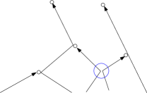
Figure 2:

The event in Figure 2 has ‘size’ $t/\mu_{\varepsilon}$ (the volume of a tube of diameter ${\varepsilon}$ and length $t$). In Chapter 4, we will give a precise definition of correlation (connection) based on geometrical constraints. It will be the elementary brick to characterize $f^{{\varepsilon}}_{n}(t)$ explicitly in terms of the initial data. The formula for $f^{{\varepsilon}}_{n}(t)$ (Section 18) will be supported on characteristic flows with $n$ particles connected, through their generated subtrees (hence of expected size $(t/\mu_{\varepsilon})^{n-1}$). In other words, while $F^{\varepsilon}_{n}$ projects the measure on arbitrary groups of particles of size $n$, the improvement of $f^{\varepsilon}_{n}$ consists in restricting to completely connected clusters of the same size.

With this naive picture in mind, let us briefly comment again on information, and irreversibility. One nice feature of the geometric analysis of dynamical correlations is that it reflects the transition from a time-reversible to a time-irreversible model. In [BGSRS18] we identified, and quantified, the microscopic singular sets where $F^{\varepsilon}_{n}$ does not converge. These sets are not invariant by time-reversal (they have a direction always pointing to the past, and not to the future). Looking at $F^{\varepsilon}_{n}(t)$, we lose track of what happens in these small sets. This implies, in particular, that Theorem 1 cannot be used to come back from time $t>0$ to the initial state at time zero. The cumulants describe what happens on all the small singular sets, therefore providing the information missing to recover the reversibility.

At the end of Chapter 4, we give a uniform estimate on these cumulants (Theorem 4), which is the main advance of this paper. This $L^{1}$-bound is sharp in ${\varepsilon}$ and $n$ ($n$-factorial bound), roughly stating that the unscaled cumulant decays as $(t/\mu_{\varepsilon})^{n-1}n^{n-2}.$ This estimate is intuitively simple. We have given a geometric notion of correlation as a link between two collision trees. Based on this notion, we can draw a random graph telling us which particles are correlated and which particles are not (each collision tree being one vertex of the graph). Since the cumulant describes $n$ completely correlated particles, there will be at least $n-1$ edges, each one of small ‘volume’ $t/\mu_{\varepsilon}$. Of course there may be more than $n-1$ connections (if the random graph has cycles), but these are hopefully unlikely as they produce extra smallness in ${\varepsilon}$. If we ignore all of them, we are left with minimally connected graphs, whose total number is $n^{n-2}$ by Cayley’s formula. Thanks to the good dependence in $n$ of these uniform bounds, we can actually sum up all the family of cumulants into an analytic series, referred to as ‘cumulant generating function’ (coinciding with formula (4.5)).

The second central result of this paper, stated in Chapter 5 (Theorem 5), is the characterization of the rescaled cumulants in the Boltzmann-Grad limit, with minimally connected graphs. Using this minimality property, we derive a Hamilton-Jacobi equation for the limiting cumulant generating function, which is our ultimate point of arrival (allowing us, in particular, to characterize the covariance of the fluctuation field and the large deviation functional).

The rest of the paper is devoted to the proofs of our main results.

Chapter 6 proves Theorem 2. Here, the uniform bounds of Theorem 4 are considerably better than what is required, and the proof amounts to looking at a characteristic function living on larger scales. Indeed a simple expansion shows that the characteristic function of the fluctuation field is determined, at leading order, by $f_{1}^{\varepsilon}$, $(\mu_{\varepsilon}^{1-\frac{n}{2}}f_{n}^{\varepsilon})_{n\geq 2}$ so that only the first two cumulants contribute to the limit. This proves the Gaussian character of the process (implying in particular the Wick Theorem for the moments of the limiting field). The more technical part of the proof concerns the tightness of the process for which we adapt a Garsia-Rodemich-Rumsey’s inequality on the modulus of continuity, to the case of a discontinuous process.

In Chapter 7 we prove Theorem 3, and actually even a slightly more general statement. Our purpose is to show that the cumulant generating function obtained in Chapter 5 is dual, through the Legendre transform, to a large deviation rate function. Restricting to the class $\mathcal{R}_{r,T}$ of observables, this rate functional can be identified with the one predicted in the literature, based on the analogy with stochastic dynamics.

Finally, Chapters 8 and 9 are devoted to the proof of Theorems 4 and 5, respectively. We encounter here a combinatorial issue. The number of terms in the formula for $f^{{\varepsilon}}_{n}(t)$ grows, at first sight, badly with $n$, and cancellations need to be exploited to obtain a factorial growth. At this point, cluster expansion methods [Ru69] (summarized in Chapter 2), applied to the collision trees, enter the game. The decay $(t/\mu_{\varepsilon})^{n-1}$ follows instead from a geometric analysis on hard-sphere trajectories with $n-1$ connecting constraints, in the spirit of previous work [BGSR2, BGSRS18, PS17].

Many different types of PDEs appear in this text, which are all solved, locally in time, by an application of an abstract Cauchy-Kovalevskaya theorem in the spirit of Nishida [nishida2]. The statement of the theorem, as well as various applications, are provided in the Appendix.

6 Remarks, and open problems

We conclude with a few remarks on our results.

• To simplify our proof, we assumed that the initial datum is a quasi-product measure, with the minimal amount of correlations (only the mutual exclusion between hard spheres is taken into account). This assumption is useful to isolate the dynamical part of the problem in the clearest way. More general initial states could be dealt with along the same lines (see [S83, PS17]). However the cumulant expansions would contain more terms, describing the deterministic (linearized) transport of initial correlations.

• Similarly, fixing only the average number of particles (instead of the exact number of particles) allows to avoid spurious correlations. We therefore work in a grand canonical setting, as is customary in statistical physics when dealing with fluctuations. Notice that fixing $\mathcal{N}=N$ produces a long range term of order $1/N$ in the covariance of the fluctuation field. Note also that the cluster expansion method, which is crucial in our analysis, is developed (with few exceptions, see [PT] for instance) in a grand canonical framework [PU09].

• Our results could be established in the whole space $\mathbb{R}^{d}$, or in a parallelepiped box with periodic or reflecting boundary conditions. Different domains might be also covered, at the expense of complications in the geometrical estimates of dynamical correlations (see [EGM11, Dolmaire, LeBihan21] for instance).

• We do not deal with the original BBGKY hierarchy of equations, which was written for smooth potentials, but always restrict to the hard-sphere system. It is plausible that our results could be extended to smooth, compactly supported potentials as considered in [GSRT, PSS17] (see [Ayi] for a fast decaying case), but the proof would be considerably more involved.

• At thermal equilibrium, we expect Theorem 2 to be true globally in time: see [BGSR2] for a first step in this direction.

Acknowledgements. We are very grateful to H. Spohn and M. Pulvirenti for many enlightening discussions on the subjects treated in this text. We thank also F. Bouchet, F. Rezakhanlou, G. Basile, D. Benedetto, L. Bertini for sharing their insights on large deviations and A. Debussche, A. de Bouard, J. Vovelle for their explanations on SPDEs. Finally, we thank the anonymous reviewers for their remarks and suggestions, which have led to a substantial improvement of our manuscript.

This work was partially supported by the ANR-15-CE40-0020-01 grant LSD. IG and LSR acknowledge the support of a grant from the Simons Foundation MPS No651463-Wave Turbulence.

Première partie Dynamical cumulants

Chapitre 2 Combinatorics on connected clusters

This preliminary chapter consists in presenting a few notions (well-known in statistical mechanics) that will be essential in our analysis: the content of this chapter is classical, but proofs are given for completeness and to prepare the less familiar reader to some of the combinatorial notions and techniques used in this article. We present in particular cumulants, and their link with exponential moments as well as with cluster expansions. We conclude the chapter with some combinatorial identities that will be useful throughout this work.

7 Generating functionals and cumulants

Let $h:\mathbb{D}\to\mathbb{R}$ be a bounded continuous function. We shall use the functional notation

$$F^{\varepsilon}_{n,t}\left(h^{\otimes n}\right)=\int_{\mathbb{D}^{n}}dZ_{n}\,F^{\varepsilon}_{n}(t,Z_{n})h(z_{1})\dots h(z_{n})\;,$$ (7.1)

(see formula (14.2) below for a generalization) and

$$\mathcal{P}^{s}_{n}=\mbox{ set of partitions of $\{1,\dots,n\}$ into $s$ parts}\;,$$

with

$$\sigma\in\mathcal{P}^{s}_{n}\Longrightarrow\sigma=\{\sigma_{1},\dots,\sigma_{s}\}\;,\quad|\sigma_{i}|=\kappa_{i}\;,\quad\sum_{i=1}^{s}\kappa_{i}=n\;.$$

The moment generating functional of the empirical measure (2.5), namely ${\mathbb{E}}_{\varepsilon}\Big{(}\exp\big{(}\pi^{\varepsilon}_{t}(h)\big{)}\Big{)}$ is related to the rescaled correlation functions (1.10) by the following remark. We recall that

$${\mathbb{E}}_{\varepsilon}\Big{(}\exp\big{(}\pi^{\varepsilon}_{t}(h)\big{)}\Big{)}={\mathbb{E}}_{\varepsilon}\left[\exp\big{(}\frac{1}{\mu_{\varepsilon}}\sum_{i=1}^{\mathcal{N}}h\big{(}{\bf z}^{{\varepsilon}}_{i}(t)\big{)}\big{)}\right]\,.$$ (7.2)

Proposition 7.1.

We have that

$${\mathbb{E}}_{\varepsilon}\Big{(}\exp\big{(}\pi^{\varepsilon}_{t}(h)\big{)}\Big{)}=1+\sum_{n=1}^{\infty}{\mu_{\varepsilon}^{n}\over n!}\,F^{\varepsilon}_{n,t}\left(\left(e^{h/\mu_{\varepsilon}}-1\right)^{\otimes n}\right)$$ (7.3)

if the series is absolutely convergent.

Démonstration.

Starting from (7.2), one has

$$\sum_{k\geq 1}{1\over k!}\,{\mathbb{E}}_{\varepsilon}\Big{(}\Big{(}\pi^{\varepsilon}_{t}(h)\Big{)}^{k}\Big{)} =\sum_{k\geq 1}{1\over k!}\,\sum_{n=1}^{k}\sum_{\sigma\in\mathcal{P}^{n}_{k}}\mu_{\varepsilon}^{-k}\,{\mathbb{E}}_{\varepsilon}\Big{(}\sum_{\begin{subarray}{c}i_{1},\dots,i_{n}\\ i_{j}\neq i_{\ell},j\neq\ell\end{subarray}}h\left({\mathbf{z}}^{\varepsilon}_{i_{1}}(t)\right)^{\kappa_{1}}\dots h\left({\mathbf{z}}^{\varepsilon}_{i_{n}}(t)\right)^{\kappa_{n}}\Big{)}$$

$$=\sum_{k\geq 1}{1\over k!}\,\sum_{n=1}^{k}\sum_{\sigma\in\mathcal{P}^{n}_{k}}\mu_{\varepsilon}^{-k}\,\mu_{\varepsilon}^{n}\int_{\mathbb{D}^{n}}dZ_{n}\,F^{{\varepsilon}}_{n}(t,Z_{n})h(z_{1})^{\kappa_{1}}\dots h(z_{n})^{\kappa_{n}}$$

where in the last equality we used (1.11). On the other hand for fixed $n$

$$\sum_{k\geq n}{\mu_{\varepsilon}^{-k}\over k!}\sum_{\sigma\in\mathcal{P}^{n}_{k}}\prod_{i=1}^{n}h(z_{i})^{\kappa_{i}} =\sum_{k\geq n}{\mu_{\varepsilon}^{-k}\over k!\,n!}\sum_{\begin{subarray}{c}\kappa_{1}\cdots\kappa_{n}\geq 1\\ \sum\kappa_{i}=k\end{subarray}}\binom{k}{\kappa_{1}}\binom{k-\kappa_{1}}{\kappa_{2}}\cdots\binom{k-\kappa_{1}-\cdots-\kappa_{n-2}}{\kappa_{n-1}}\prod_{i=1}^{n}h(z_{i})^{\kappa_{i}}$$

$$={1\over n!}\prod_{i=1}^{n}\sum_{\kappa_{i}\geq 1}{h(z_{i})^{\kappa_{i}}\over\mu_{\varepsilon}^{\kappa_{i}}\kappa_{i}!}={1\over n!}\prod_{i=1}^{n}\left(e^{h(z_{i})/\mu_{\varepsilon}}-1\right)\;.$$

Therefore

$${\mathbb{E}}_{\varepsilon}\left(\exp\Big{(}\pi^{\varepsilon}_{t}(h)\Big{)}\right)=1+\sum_{n\geq 1}\mu_{\varepsilon}^{n}\int_{\mathbb{D}^{n}}dZ_{n}\,F^{{\varepsilon}}_{n}(t,Z_{n}){1\over n!}\prod_{i=1}^{n}\left(e^{h(z_{i})/\mu_{\varepsilon}}-1\right)\;,$$

which proves the proposition. ∎

The moment generating functional is just a compact representation of the information coded in the family $\left(F^{{\varepsilon}}_{n}(t)\right)_{n\geq 1}$. After the Boltzmann-Grad limit $\mu_{\varepsilon}\to\infty$, the right-hand side of (7.3) reduces to $\displaystyle\sum_{n=0}^{\infty}{1\over n!}\Big{(}\int f(t)h\Big{)}^{n}=\exp\Big{(}\int f(t)h\Big{)}$, i.e. to the solution of the Boltzmann equation.

As discussed in the introduction, our purpose is to keep a much larger amount of information. To this end, we study the cumulant generating functional which is, by Cramér’s theorem, an obvious candidate to reach atypical profiles [Varadhan]. Namely, we pass to the logarithm and rescale as follows:

$$\Lambda^{\varepsilon}_{t}(e^{h}):=\frac{1}{\mu_{\varepsilon}}\log{\mathbb{E}}_{\varepsilon}\left(\exp\Big{(}\mu_{\varepsilon}\,\pi^{\varepsilon}_{t}(h)\Big{)}\right)=\frac{1}{\mu_{\varepsilon}}\log{\mathbb{E}}_{\varepsilon}\Big{(}\exp\big{(}\sum_{i=1}^{\mathcal{N}}h\big{(}{\bf z}^{{\varepsilon}}_{i}(t)\big{)}\big{)}\Big{)}\;.$$ (7.4)

The first task is to look for a proposition analogous to the previous one. In doing so, the following definition emerges naturally, where we use the notation:

$$G_{\sigma_{j}}:=G_{|\sigma_{j}|}(Z_{\sigma_{j}})\,,\quad G_{\sigma}:=\prod_{j=1}^{|\sigma|}G_{\sigma_{j}}$$ (7.5)

for $\sigma=\{\sigma_{1},\dots,\sigma_{s}\}\in\mathcal{P}^{s}_{n}$.

Definition 7.2 (Cumulants).

Let $(G_{n})_{n\geq 1}$ be a family of distributions of $n$ variables invariant by permutation of the labels of the variables. The rescaled cumulants associated with $(G_{n})_{n\geq 1}$ form the family $(g_{n})_{n\geq 1}$ defined, for all $n\geq 1$, by

$$g_{n}=\mu_{\varepsilon}^{n-1}\sum_{s=1}^{n}\sum_{\sigma\in\mathcal{P}^{s}_{n}}(-1)^{s-1}(s-1)!\,G_{\sigma}\,.$$ (7.6)

The scaling factor $\mu_{\varepsilon}^{n-1}$ (although unnecessary in this chapter) is introduced for later convenience, and will ensure that the cumulants are of order $1$ in $\varepsilon$.

We then have the following result, which is well-known in the theory of point processes (see [daley]).

Proposition 7.3.

Let $(f^{\varepsilon}_{n})_{n\geq 1}$ be the family of rescaled cumulants associated with $\left(F^{\varepsilon}_{n}\right)_{n\geq 1}$. We have

$$\Lambda^{\varepsilon}_{t}(e^{h})=\sum_{n=1}^{\infty}{1\over n!}f^{\varepsilon}_{n,t}\left(\left(e^{h}-1\right)^{\otimes n}\right)\;,$$

if the series is absolutely convergent.

Démonstration.

Applying Proposition 7.1 to $h$ in place of $h/\mu_{\varepsilon}$, expanding the logarithm in a series and using Definition 7.2, we get

$$\frac{1}{\mu_{\varepsilon}}\log{\mathbb{E}}_{\varepsilon}\left(\exp\Big{(}\mu_{\varepsilon}\,\pi^{\varepsilon}_{t}(h)\Big{)}\right) =\frac{1}{\mu_{\varepsilon}}\sum_{n=1}^{\infty}{(-1)^{n-1}\over n}\prod_{\ell=1}^{n}\left[\sum_{p_{\ell}}{\mu_{\varepsilon}^{p_{\ell}}\over p_{\ell}!}F^{\varepsilon}_{p_{\ell},t}\left((e^{h}-1)^{\otimes p_{\ell}}\right)\right]$$

$$=\frac{1}{\mu_{\varepsilon}}\sum_{n=1}^{\infty}{(-1)^{n-1}\over n}\sum_{p_{1},\dots,p_{n}}{\mu_{\varepsilon}^{p_{1}+\dots+p_{n}}\over p_{1}!\dots p_{n}!}\prod_{\ell=1}^{n}F^{\varepsilon}_{p_{\ell},t}\left((e^{h}-1)^{\otimes p_{\ell}}\right)$$

$$=\sum_{p=1}^{\infty}\frac{\mu_{\varepsilon}^{p-1}}{p!}\sum_{n=1}^{p}\sum_{\sigma\in\mathcal{P}^{n}_{p}}(-1)^{n-1}(n-1)!\prod_{\ell=1}^{n}F^{\varepsilon}_{p_{\ell},t}\left((e^{h}-1)^{\otimes p_{\ell}}\right)$$

$$=\sum_{p=1}^{\infty}{1\over p!}f^{\varepsilon}_{p,t}\left(\left(e^{h}-1\right)^{\otimes p}\right)\;.$$

In the third equality, we used that the number of partitions of $\{1,\dots,p\}$ into $n$ sets with cardinals $p_{1},\dots,p_{n}$ is given by

$$\left|\mathcal{P}_{p}^{n}(p_{1},\dots,p_{n})\right|=\frac{1}{n!}\;\binom{p}{p_{1}}\binom{p-p_{1}}{p_{2}}\cdots\binom{p-p_{1}-\cdots-p_{n-1}}{p_{n}}=\frac{1}{n!}\;\frac{p!}{p_{1}!\;\cdots\;p_{n}!}\,,$$ (7.7)

where the factor $n!$ arises to take into account the fact that the sets of the partition are not ordered. This proves the result. ∎

Note that cumulants measure departure from chaos in the sense that they vanish identically at order $n\geq 2$ in the case of i.i.d. random variables.

8 Inversion formula for cumulants

In this section we prove that the cumulants $(g_{n})$ associated with a family $(G_{n})$ in the sense of Definition 7.2, encode all the correlations, meaning that $G_{n}$ can be reconstructed from $(g_{k})_{k\leq n}$ for all $n\geq 1$. More precisely, the following inversion formula holds.

Proposition 8.1.

Let $(G_{n})_{n\geq 1}$ be a family of distributions and $(g_{n})_{n\geq 1}$ its cumulants in the sense of Definition 7.2. Then the map from $(G_{n})_{n\geq 1}$ to its cumulants $(g_{n})_{n\geq 1}$ is a bijection and, for each $n\geq 1$, the distribution $G_{n}$ can be recovered from the cumulants $(g_{k})_{k\leq n}$ by the inversion formula

$$\forall n\geq 1\,,\qquad G_{n}=\sum_{s=1}^{n}\sum_{\sigma\in\mathcal{P}_{n}^{s}}\;\mu_{\varepsilon}^{-(n-s)}g_{\sigma}\,.$$ (8.1)

Equations (8.1) and (7.6) are equivalent definitions of $(g_{n})_{n\geq 1}$.

Démonstration.

Let us check that

$$G_{n}=\mu_{\varepsilon}^{-(n-1)}g_{n}+\sum_{s=2}^{n}\mu_{\varepsilon}^{-(n-s)}\sum_{\sigma\in\mathcal{P}_{n}^{s}}g_{\sigma}\,.$$

Replacing the cumulants $g_{\sigma_{j}}$ by their definition, we get

$${\mathbb{A}}_{n}:=\sum_{s=2}^{n}\sum_{\sigma\in\mathcal{P}_{n}^{s}}\mu_{\varepsilon}^{-(n-s)}g_{\sigma}=\sum_{s=2}^{n}\sum_{\sigma\in\mathcal{P}_{n}^{s}}\prod_{j=1}^{s}\Big{(}\sum_{k_{j}=1}^{|\sigma_{j}|}\sum_{\kappa_{j}\in\mathcal{P}_{\sigma_{j}}^{k_{j}}}(-1)^{k_{j}-1}(k_{j}-1)!\;G_{\kappa_{j}}\Big{)}\,.$$

Using the Fubini Theorem, we can index the sum by the partitions with $r:=\displaystyle\sum_{j=1}^{s}k_{j}$ sets and obtain

$${\mathbb{A}}_{n}=\sum_{r=2}^{n}\sum_{\rho\in\mathcal{P}_{n}^{r}}G_{\rho}\Big{(}\sum_{s=2}^{r}\sum_{\omega\in\mathcal{P}_{r}^{s}}(-1)^{r-s}\prod_{i=1}^{s}(|\omega_{i}|-1)!\Big{)}\,.$$

Note that the partition $\sigma$ in the definition of ${\mathbb{A}}_{n}$ can be recovered as

$$\forall i\leq s\,,\qquad\sigma_{i}=\bigcup_{j\in\omega_{i}}\rho_{j}\,.$$

Using the combinatorial identity

$$\sum_{k=1}^{n}\sum_{\sigma\in\mathcal{P}_{n}^{k}}(-1)^{k}\prod_{i=1}^{k}(|\sigma_{i}|-1)!=0$$

(see Lemma 11.1 below for a proof), we find that

$$\sum_{s=2}^{r}\sum_{\omega\in\mathcal{P}_{r}^{s}}(-1)^{r-s}\prod_{i=1}^{s}(|\omega_{i}|-1)!=-(-1)^{r-1}(r-1)!\,,$$

hence it follows that

$${\mathbb{A}}_{n} =-\sum_{r=2}^{n}\sum_{\rho\in\mathcal{P}_{n}^{r}}G_{\rho}(-1)^{r-1}(r-1)!=-\mu_{\varepsilon}^{-(n-1)}g_{n}+G_{n}\,,$$

where the last equality follows from the definition of $g_{n}$. Similarly, (8.1) $\Rightarrow$ (7.6) can be verified by induction on $n$. This completes the proof of Proposition 8.1. ∎

9 Clusters and the tree inequality

We now prove that the cumulant of order $n$ is supported on clusters (connected groups) of cardinality $n$. We shall consider an abstract situation based on a “disconnection” condition, the definition of which may change according to the context.

Definition 9.1.

A connection is a commutative binary relation $\sim$ on a set $V$:

$$x\sim y\;,\quad x,y\in V\;.$$

The (commutative) complementary relation, called disconnection, is denoted $\not\sim$, that is $x\not\sim y$ if and only if $x\sim y$ is false.

Consider the indicator function that $n$ elements $\{\eta_{1},\dots,\eta_{n}\}$ are disconnected

$$\Phi_{n}\big{(}\eta_{1},\dots,\eta_{n}\big{)}:=\prod_{1\leq i\not=j\leq n}{\bf 1}_{\eta_{i}\not\sim\eta_{j}}\,.$$

For $n=1$, we set $\Phi_{1}\big{(}\eta_{1})\equiv 1$.

The following proposition shows that the cumulant of order $n$ of $\Phi_{n}$ is supported on clusters of length $n$, meaning configurations $(\eta_{1},\dots,\eta_{n})$ in which all elements are linked by a chain of connected elements. Before stating the proposition let us recall some classical terminology on graphs. This definition, as well as Proposition 9.3 and its proof, are taken from [gibbspp].

Definition 9.2.

Let $V$ be a set of vertices and $E\subset\big{\{}\{v,w\},\;v,w\in V\,,\;v\neq w\big{\}}$ a set of edges. The pair $G=(V,E)$ is called a graph (undirected, no self-edge, no multiple edge). Given a graph $G$ we denote by $E(G)$ the set of all edges in $G$. The graph is said connected if for all $v,w\in V$, $v\neq w$, there exist $v_{0}=v,v_{1},v_{2},\dots,v_{n}=w$ such that $\{v_{i-1},v_{i}\}\in E$ for all $i=1,\dots,n$.

We denote by $\mathcal{C}_{V}$ the set of connected graphs with $V$ as vertices, and by $\mathcal{C}_{n}$ the set of connected graphs with $n$ vertices when $V=\{1,\dots,n\}$. A minimally connected, or tree graph, is a connected graph with $n-1$ edges. We denote by $\mathcal{T}_{V}$ the set of minimally connected graphs with $V$ as vertices, and by $\mathcal{T}_{n}$ the set of minimally connected graphs with $n$ vertices when $V=\{1,\dots,n\}$.

Finally, the union of two graphs $G_{1}=(V_{1},E_{1})$ and $G_{2}=(V_{2},E_{2})$ is $G_{1}\cup G_{2}=(V_{1}\cup V_{2},E_{1}\cup E_{2})$.

The following result was originally derived by Penrose [Pe67].

Proposition 9.3.

The (unrescaled) cumulant of $\Phi_{n}$ defined as in Definition 7.2 is equal to

$$\varphi_{n}\big{(}\eta_{1},\dots,\eta_{n}\big{)}=\sum_{G\in\mathcal{C}_{n}}\prod_{\{i,j\}\in E(G)}(-{\bf 1}_{\eta_{i}\sim\eta_{j}})\,.$$ (9.1)

Furthermore, one has the following “tree inequality”

$$|\varphi_{n}\big{(}\eta_{1},\dots,\eta_{n}\big{)}|\leq\sum_{T\in\mathcal{T}_{n}}\prod_{\{i,j\}\in E(T)}{\bf 1}_{\eta_{i}\sim\eta_{j}}\,.$$ (9.2)

Démonstration.

The first step is to check the representation formula (9.1) for the cumulant $\varphi_{n}$. The starting point is the definition of $\Phi_{n}$

$$\Phi_{n}\big{(}\eta_{1},\dots,\eta_{n}\big{)}=\prod_{1\leq i\not=j\leq n}(1-{\bf 1}_{\eta_{i}\sim\eta_{j}})=\sum_{G}\prod_{\{i,j\}\in E(G)}(-{\bf 1}_{\eta_{i}\sim\eta_{j}})\,,$$

where the sum over $G$ runs over all graphs with $n$ vertices. We then decompose these graphs into connected components and obtain that

$$\Phi_{n}\big{(}\eta_{1},\dots,\eta_{n}\big{)}=\sum_{s=1}^{n}\sum_{\sigma\in\mathcal{P}^{s}_{n}}\prod_{k=1}^{s}\left(\sum_{G_{k}\in\mathcal{C}_{\sigma_{k}}}\prod_{\{i,j\}\in E(G_{k})}(-{\bf 1}_{\eta_{i}\sim\eta_{j}})\right)\,.$$

By the uniqueness of the cumulant decomposition as given in Proposition 8.1 (without the rescaling), we therefore find (9.1).

The second step is to compare connected graphs and trees. This is achieved by defining a tree partition scheme, i.e. a map $\pi:\mathcal{C}_{n}\to\mathcal{T}_{n}$ such that for any $T\in\mathcal{T}_{n}$, there is a graph $R(T)\in\mathcal{C}_{n}$ satisfying

$$\pi^{-1}(\{T\})=\big{\{}G\in\mathcal{C}_{n}\,:\,E(T)\subset E(G)\subset E(R(T))\big{\}}\,.$$

Penrose’s partition scheme is obtained in the following way. Given a graph $G$, we define its image $T$ iteratively starting from the root $1$

• the first generation of $T$ consists of all $i$ such that $\{1,i\}\in G$; these vertices are accepted and labeled in increasing order $t_{1,1},\dots,t_{1,r_{1}}$;

• the $\ell$-th generation consists of all $i$ which are not already in the tree, and such that $\{t_{\ell-1,j},i\}$ belongs to $E(G)$ for some $j\in\{1,\dots,r_{\ell-1}\}$; these vertices are labeled in increasing order of $j=1,\dots,r_{\ell-1}$, then increasing order of $i$.

The procedure ends with a unique tree $T\in\mathcal{T}_{n}$. In order to characterize $R(T)$, we now investigate which edges of $G$ have been discarded. Denote by $d(i)$ the graph distance of the vertex $i$ to the root (which is just its generation). Let $\{i,j\}\in E(G)\setminus E(T)$ and assume without loss of generality that $d(i)\leq d(j)$. By construction $d(j)\leq d(i)+1$. Furthermore, if $d(j)=d(i)+1$, the parent $i^{\prime}$ of $j$ in the tree is such that $i^{\prime}<i$. Therefore $E(G)\setminus E(T)$ is a subset of the set $E^{\prime}(T)$ consisting of edges within a generation ($d(i)=d(j)$), and of edges towards a younger uncle ($d(j)=d(i)+1$ and $i^{\prime}<i$). Conversely, we can check that any graph satisfying $E(T)\subset G\subset E(T)\cup E^{\prime}(T)$ belongs to $\pi^{-1}(\{T\})$. We therefore define $R(T)$ as the graph with edges $E(T)\cup E^{\prime}(T)$.

The last step is to exploit the non trivial cancellations between graphs associated with the same tree. There holds, with the above notation,

$$\sum_{G\in\mathcal{C}_{n}}\prod_{\{i,j\}\in E(G)}(-{\bf 1}_{\eta_{i}\sim\eta_{j}}) =\sum_{T\in\mathcal{T}_{n}}\sum_{G\in\pi^{-1}(T)}\prod_{\{i,j\}\in E(G)}(-{\bf 1}_{\eta_{i}\sim\eta_{j}})$$

$$=\sum_{T\in\mathcal{T}_{n}}\left(\prod_{\{i,j\}\in E(T)}(-{\bf 1}_{\eta_{i}\sim\eta_{j}})\right)\left(\sum_{E^{\prime}\subset E^{\prime}(T)}\prod_{\{i,j\}\in E^{\prime}}(-{\bf 1}_{\eta_{i}\sim\eta_{j}})\right)$$

$$=\sum_{T\in\mathcal{T}_{n}}\left(\prod_{\{i,j\}\in E(T)}(-{\bf 1}_{\eta_{i}\sim\eta_{j}})\right)\left(\prod_{\{i,j\}\in E^{\prime}(T)}(1-{\bf 1}_{\eta_{i}\sim\eta_{j}})\right)\,.$$

The conclusion follows from the fact that $(1-{\bf 1}_{\eta_{i}\sim\eta_{j}})\in[0,1]$. The proposition is proved. ∎

10 Number of minimally connected graphs

The following classical result will be used in Chapter 8.

Lemma 10.1.

The cardinality of the set of minimally connected graphs on $n$ vertices with degrees (number of edges per vertex) of the vertices $1,\dots,n$ fixed respectively at the values $d_{1},\dots,d_{n}$ is

$$\Big{|}\Big{\{}T\in\mathcal{T}_{n}\;\;:\;\;d_{1}(T)=d_{1},\dots,d_{n}(T)=d_{n}\Big{\}}\Big{|}=\frac{(n-2)!}{\prod_{i=1}^{n}(d_{i}-1)!}\,\cdotp$$ (10.1)

Before proving the lemma, let us notice that it implies Cayley’s formula $|\mathcal{T}_{n}|=n^{n-2}$. Indeed the graph is minimal, so there are exactly $n-1$ edges hence (each edge has two vertices) the sum of the degrees has to be equal to $2n-2$. Thus

$$|\mathcal{T}_{n}|=\sum_{\begin{subarray}{c}d_{1},\dots,d_{n}\\ 1\leq d_{i}\leq n-1\\ \sum_{i}d_{i}=2(n-1)\end{subarray}}\frac{(n-2)!}{\prod_{i=1}^{n}(d_{i}-1)!}=\sum_{\begin{subarray}{c}d_{1},\dots,d_{n}\\ 0\leq d_{i}\leq n-2\\ \sum_{i}d_{i}=n-2\end{subarray}}\frac{(n-2)!}{\prod_{i=1}^{n}d_{i}!}=\left(\sum_{i=1}^{n}\,1\right)^{n-2}\;.$$

Démonstration.

The lemma can be proved by induction. For $n=2$ the result is trivial, so we suppose to have proved it for the set $\mathcal{T}_{n}^{d_{1},\dots,d_{n}}:=\{T\in\mathcal{T}_{n}\;\;|\;\;d_{1}(T)=d_{1},\dots,d_{n}(T)=d_{n}\}$, for arbitrary $d_{1},\dots,d_{n}$, and consider the set $\mathcal{T}_{n+1}^{d_{1},\dots,d_{n+1}}$. Since there is always at least one vertex of degree 1, we can assume without loss of generality that $d_{n+1}=1$. Notice that, if the vertex $n+1$ is linked to the vertex $j$, then necessarily $d_{j}\geq 2$. We therefore compute the number of minimally connected graphs on $n$ vertices with degrees $d_{1},\dots,d_{j-1},d_{j}-1,d_{j+1},\dots,d_{n}$, and sum then over $j$ (all the ways to attach the vertex $n+1$ of degree 1). This leads to

$$|\mathcal{T}_{n+1}^{d_{1},\dots,d_{n+1}}|=\sum_{j=1}^{n}\frac{(n-2)!}{(d_{j}-2)!\prod_{i\neq j}(d_{i}-1)!}\,,$$

hence

$$|\mathcal{T}_{n+1}^{d_{1},\dots,d_{n+1}}|=\frac{(n-2)!}{\prod_{i=1}^{n+1}(d_{i}-1)!}\sum_{j=1}^{n+1}(d_{j}-1)=\frac{(n-1)!}{\prod_{i=1}^{n}(d_{i}-1)!}$$

having used again $\sum_{j=1}^{n+1}d_{j}=2(n+1-1)$. ∎

11 Combinatorial identities

The following combinatorial identities have been used in the previous sections.

Lemma 11.1.

For $n\geq 2$ there holds

$$\sum_{k=1}^{n}\sum_{\sigma\in\mathcal{P}_{n}^{k}}(-1)^{k}(k-1)!=0\,,$$ (11.1)

$$\sum_{k=1}^{n}\sum_{\sigma\in\mathcal{P}_{n}^{k}}(-1)^{k}\prod_{i=1}^{k}(|\sigma_{i}|-1)!=0\,.$$ (11.2)

Démonstration.

From the Taylor series of $x\mapsto\log\big{(}\exp(x)\big{)}$, we deduce that

$$\forall n\geq 2,\qquad\sum_{k=1}^{n}\sum_{\ell_{1}+\dots+\ell_{k}=n}\frac{(-1)^{k}}{k}\;\frac{1}{\ell_{1}!\dots\ell_{k}!}=0\,.$$

Combining (7.7) and the previous identity, we get

$$0=\sum_{k=1}^{n}\sum_{\ell_{1}+\dots+\ell_{k}=n}\frac{(-1)^{k}}{k}\;\frac{1}{\ell_{1}!\dots\ell_{k}!} =\sum_{k=1}^{n}\frac{(-1)^{k}}{k}\sum_{\ell_{1}+\dots+\ell_{k}=n}{k!\over n!}\sharp\mathcal{P}_{n}^{k}(\ell_{1},\dots,\ell_{k})$$

$$={1\over n!}\sum_{k=1}^{n}(-1)^{k}(k-1)!\sharp\mathcal{P}_{n}^{k}$$

and this completes the first identity (11.1).

From the Taylor series of $x\mapsto\exp\big{(}\log(1+x)\big{)}$, we deduce that

$$\forall n\geq 2,\qquad\sum_{k=1}^{n}\frac{1}{k!}\sum_{\ell_{1}+\dots+\ell_{k}=n}\frac{(-1)^{k}}{\ell_{1}\dots\ell_{k}}=0\,.$$

Combining (7.7) and the previous identity, we get

$$0=\sum_{k=1}^{n}\frac{1}{k!}\sum_{\ell_{1}+\dots+\ell_{k}=n}\frac{(-1)^{k}}{\ell_{1}\dots\ell_{k}}=\frac{1}{n!}\sum_{k=1}^{n}\sum_{\sigma\in\mathcal{P}_{n}^{k}}(-1)^{k}\prod_{i=1}^{k}(|\sigma_{i}|-1)!$$

and this completes the second identity (11.2).

The lemma is proved. ∎

Chapitre 3 Tree expansions of the hard-sphere dynamics

Here and in the next chapter, we explain how the combinatorial methods presented in the previous chapter can be applied to study the dynamical correlations of hard spheres. The first steps in this direction are to define a suitable family describing the correlations of order $n$, and then to obtain a graphical representation of this family which will be helpful to identify the clustering structure.

12 Space correlation functions

For the sake of simplicity, we start by describing correlations in phase space. Recall that the $n$-particle correlation function $F^{\varepsilon}_{n}\equiv F^{\varepsilon}_{n}(t,Z_{n})$ defined by (1.10) counts how many groups of $n$ particles are, in average, in a given configuration $Z_{n}$ at time $t$: see Eq. (1.11).

Let us now discuss the time evolution of the correlation functions: by integration of the Liouville equation (1.3), we get that the family $(F_{n}^{\varepsilon})_{n\geq 1}$ satisfies the so-called BBGKY hierarchy (going back to [Ce72]) :

$$\partial_{t}F^{\varepsilon}_{n}+V_{n}\cdot\nabla_{X_{n}}F^{\varepsilon}_{n}=C^{\varepsilon}_{n,n+1}F^{\varepsilon}_{n+1}\quad\mbox{in}\quad{\mathcal{D}}^{\varepsilon}_{n}$$ (12.1)

with specular boundary reflection

$$\forall Z_{n}\in{\partial}{\mathcal{D}}^{{\varepsilon}+}_{n}(i,j)\,,\quad F^{\varepsilon}_{n}(t,Z_{n}):=F^{\varepsilon}_{n}(t,Z_{n}^{{}^{\prime}i,j})\,,$$ (12.2)

where $Z^{{}^{\prime}i,j}_{N}$ differs from $Z_{N}$ only by (1.2). The collision operator in the right-hand side of (12.1) comes from the boundary terms in Green’s formula (using the reflection condition to rewrite the gain part in terms of pre-collisional velocities):

$$C^{\varepsilon}_{n,n+1}F^{\varepsilon}_{n+1}:=\sum_{i=1}^{n}C_{n,n+1}^{i,{\varepsilon}}F^{\varepsilon}_{n+1}$$

with

$$(C_{n,n+1}^{i,{\varepsilon}}F^{\varepsilon}_{n+1})(Z_{n}):=\int F^{\varepsilon}_{n+1}(Z_{n}^{\langle i\rangle},x_{i},v^{\prime}_{i},x_{i}+{\varepsilon}\omega,w^{\prime})\big{(}(w-v_{i})\cdot\omega\big{)}_{+}\,d\omega dw$$ (12.3)

$$-\int F^{\varepsilon}_{n+1}(Z_{n},x_{i}+{\varepsilon}\omega,w)\big{(}(w-v_{i})\cdot\omega\big{)}_{-}\,d\omega dw\,,$$

where $(v^{\prime}_{i},w^{\prime})$ is recovered from $(v_{i},w)$ through the scattering laws (1.2), and with the notation

$$Z_{n}^{\langle i\rangle}:=(z_{1},\dots,z_{i-1},z_{i+1},\dots,z_{n})\,.$$ (12.4)

Note that the collision operator is defined as a trace, and thus some regularity on $F^{\varepsilon}_{n+1}$ is required to make sense of this operator. The classical way of dealing with this issue (see for instance [GSRT, S]) is to consider the integrated form of the equation, obtained by Duhamel’s formula

$$F^{\varepsilon}_{n}(t)=S^{\varepsilon}_{n}(t)F_{n}^{{\varepsilon}0}+\int_{0}^{t}S^{\varepsilon}_{n}(t-t_{1})C^{\varepsilon}_{n,n+1}F^{\varepsilon}_{n+1}(t_{1})dt_{1}\,,$$

denoting by $S^{\varepsilon}_{n}$ the group associated with free transport in $\mathcal{D}^{\varepsilon}_{n}$ with specular reflection on the boundary ${\partial}\mathcal{D}^{\varepsilon}_{n}$.

Iterating Duhamel’s formula, we can express the solution as a sum of operators acting on the initial data :

$$F^{\varepsilon}_{n}(t)=\sum_{m\geq 0}Q^{\varepsilon}_{n,n+m}(t)F_{n+m}^{{\varepsilon}0}\,,$$ (12.5)

where we have defined for $t>0$

$$Q^{\varepsilon}_{n,n+m}(t)F_{n+m}^{{\varepsilon}0}:=\int_{0}^{t}\int_{0}^{t_{1}}\dots\int_{0}^{t_{m-1}}S^{\varepsilon}_{n}(t-t_{1})C^{\varepsilon}_{n,n+1}S^{\varepsilon}_{n+1}(t_{1}-t_{2})C^{\varepsilon}_{n+1,n+2}$$ (12.6)

$$\dots S^{\varepsilon}_{n+m}(t_{m})F_{n+m}^{{\varepsilon}0}\>dt_{m}\dots dt_{1}$$

and $Q^{\varepsilon}_{n,n}(t)F^{{\varepsilon}0}_{n}:=S^{\varepsilon}_{n}(t)F_{n}^{{\varepsilon}0}$, $Q^{\varepsilon}_{n,n+m}(0)F^{{\varepsilon}0}_{n+m}:=\delta_{m,0}F^{{\varepsilon}0}_{n+m}$.

13 Geometrical representation with collision trees

The usual way to study the Duhamel series (12.5) is to introduce “pseudo-dynamics” describing the action of the operator $Q^{\varepsilon}_{n,n+m}$. In the following, particles will be denoted by two different types of labels: either integers $i$ or labels $i*$ (this difference will correspond to the fact that particles labeled with an integer $i$ will be added to the pseudo-dynamics through the Duhamel formula as time goes backwards, while those labeled by $i*$ are already present at time $t$). The configuration of the particle labeled $i*$ will be denoted indifferently $z_{i}^{*}=(x_{i}^{*},v_{i}^{*})$ or $z_{i*}=(x_{i*},v_{i*})$.

Definition 13.1 (Collision trees).

Given $n\geq 1\,,m\geq 0$, an (ordered) collision tree $a\in\mathcal{A}_{n,m}$ is a family $(a_{i})_{1\leq i\leq m}$ with $a_{i}\in\{1,\dots,i-1\}\cup\{1*,\dots,n*\}$.

Note that  $|\mathcal{A}_{n,m}|=n(n+1)\dots(n+m-1)$.

Given a collision tree $a\in\mathcal{A}_{n,m}$, we define pseudo-dynamics starting from a configuration $Z_{n}^{*}=(x_{i}^{*},v_{i}^{*})_{1\leq i\leq n}$ in the $n$-particle phase space at time $t$ as follows.

Definition 13.2 (Pseudo-trajectory).

Given $Z_{n}^{*}\in\mathcal{D}^{\varepsilon}_{n}$, $m\in\mathbb{N}$ and $a\in\mathcal{A}_{n,m}$, we consider a collection of times, angles and velocities $(T_{m},\Omega_{m},V_{m}):=(t_{i},\omega_{i},v_{i})_{1\leq i\leq m}$ satisfying the constraint

$$0\leq t_{m}<\cdots<t_{1}\leq t=t_{0}\,.$$

We define recursively pseudo-trajectories as follows:

• in between the collision times $t_{i}$ and $t_{i+1}$ the particles follow the $(n+i)$-particle (backward) hard-sphere flow;

• at time $t_{i}^{+}$, particle $i$ is adjoined to particle $a_{i}$ at position $x_{a_{i}}+{\varepsilon}\omega_{i}$ and with velocity $v_{i}$, provided it remains at a distance larger than ${\varepsilon}$ from all the other particles. If $(v_{i}-v_{a_{i}}(t_{i}^{+}))\cdot\omega_{i}>0$, velocities at time $t_{i}^{-}$ are given by the scattering laws

  $$v_{a_{i}}(t^{-}_{i}) :=v_{a_{i}}(t_{i}^{+})-\left((v_{a_{i}}(t_{i}^{+})-v_{i})\cdot\omega_{i}\right)\,\omega_{i}\,,$$ (13.1)

  $$v_{i}(t^{-}_{i}) :=v_{i}+\left((v_{a_{i}}(t_{i}^{+})-v_{i})\cdot\omega_{i}\right)\,\omega_{i}\,.$$

We denote by $\Psi^{\varepsilon}_{n,m}=\Psi^{\varepsilon}_{n,m}(t)$ (we shall sometimes omit to emphasize the number of created particles and denote it simply by $\Psi^{\varepsilon}_{n}$) the so constructed pseudo-trajectory, and by $Z_{n,m}(\tau)=\big{(}Z_{n}^{*}(\tau),Z_{m}(\tau)\big{)}$ the coordinates of the particles in the pseudo-trajectory at time $\tau\leq t_{m}$. It depends on the parameters $a,Z_{n}^{*},T_{m},\Omega_{m},V_{m}$, and $t$. We also define $\mathcal{G}_{m}^{{\varepsilon}}(a,Z_{n}^{*})$ to be the set of parameters $(T_{m},\Omega_{m},V_{m})$ such that the pseudo-trajectory exists up to time $0$, meaning in particular that on adjunction of a new particle, its distance to the others remains larger than ${\varepsilon}$. For $m=0$, there is no adjoined particle and the pseudo-trajectory $\Psi^{\varepsilon}_{n,0}(\tau)=Z_{n,0}(\emptyset,Z_{n}^{*},\tau)$ for $\tau\in(0,t)$ is the $n$-particle (backward) hard-sphere flow.

For a given time $t>0$, the sample path pseudo-trajectory of the $n$ ($*-$labeled) particles is denoted by ${Z}_{n}^{*}([0,t])$.

Remark 13.3.

We stress the difference in notation: “$z_{i}(\tau)$” in the above definition denotes the configuration of particle $i$ in the pseudo-trajectory while the real, $\mathcal{N}$-particle hard-sphere flow is denoted ${\mathbf{Z}}^{\varepsilon}_{\mathcal{N}}(\tau)$ as in (1.7): particle $i$ has configuration ${\mathbf{z}}^{\varepsilon}_{i}(\tau)$ in the hard-sphere flow.

With these notations, the representation formula (12.5) for the $n$-particle correlation function can be rewritten as

$$F^{\varepsilon}_{n}(t,Z_{n}^{*})=\sum_{m\geq 0}\,\sum_{a\in\mathcal{A}_{n,m}}\,\int_{\mathcal{G}_{m}^{{\varepsilon}}(a,Z_{n}^{*})}dT_{m}d\Omega_{m}dV_{m}\,\Big{(}\prod_{i=1}^{m}\big{(}v_{i}-v_{a_{i}}(t_{i})\big{)}\cdot\omega_{i}\Big{)}\,F_{n+m}^{{\varepsilon}0}\big{(}\Psi^{{\varepsilon}0}_{n,m}\big{)}\,,$$ (13.2)

where

$$dT_{m}:=dt_{1}\dots dt_{m}\,{\mathbf{1}}_{0\leq t_{m}\leq\dots\leq t_{1}\leq t}\,,$$

we have denoted by $(F_{n}^{{\varepsilon}0})_{n\geq 1}$ the initial rescaled correlation function, and $\Psi^{{\varepsilon}0}_{n,m}$ is the configuration at time 0 associated with the pseudo-trajectory $\Psi^{\varepsilon}_{n,m}$. Note that the variables $\omega_{i}$ are integrated over spheres and the scalar products take positive and negative values (corresponding to the positive and negative parts of the collision operators). Equivalently, we can introduce decorated trees $\left(a,s_{1},\dots,s_{m}\right)$ with signs $s_{i}=\pm$ specifying the collision hemispheres: denoting by $\mathcal{A}_{n,m}^{\pm}$ the set of all such trees, we can write Eq. (13.2) as

$$F^{\varepsilon}_{n}(t,Z_{n}^{*})=\sum_{m\geq 0}\,\sum_{a\in\mathcal{A}^{\pm}_{n,m}}\,\int_{\mathcal{G}_{m}^{{\varepsilon}}(a,Z_{n}^{*})}dT_{m}d\Omega_{m}dV_{m}\,\Big{(}\prod_{i=1}^{m}s_{i}\left(\big{(}v_{i}-v_{a_{i}}(t_{i})\big{)}\cdot\omega_{i}\right)_{+}\Big{)}\,F_{n+m}^{{\varepsilon}0}\big{(}\Psi^{{\varepsilon}0}_{n,m}\big{)}\,,$$ (13.3)

where the pseudo-trajectory is defined as before, with the scattering (13.1) applied in the case $s_{i}=+$ and the creation at position $x_{i}+s_{i}{\varepsilon}\omega_{i}$.

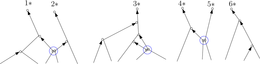
Figure 3: An example of pseudo-trajectory with $n=6$, $m=10$. In this symbolic picture, time is thought of as flowing upwards (at the top we have a configuration $Z_{6}^{*}$, at the bottom $\Psi^{{\varepsilon}0}_{6,10}$). The little circles represent hard spheres of diameter ${\varepsilon}$. Notice that several collisions are possible between the adjunction times $T_{m}$. These collisions are highlighted by blue circles. For simplicity, the hard spheres have been drawn only at their first time of existence (going backwards), and at collisions between adjunction times.

14 Averaging over trajectories

To describe dynamical correlations more precisely, we are going to follow the particle trajectories. As noted in Remark 13.3, pseudo-trajectories provide a geometric representation of the iterated Duhamel series (12.5), but they are not physical trajectories of the particle system. Nevertheless, the probability on the trajectories of $n$ particles can be derived from the Duhamel series, as we are going to explain now.

For a given time $t>0$, the sample path of $n$ particles labeled $i_{1}$ to $i_{n}$, among the ${\mathcal{N}}$ hard spheres, is denoted $({\bf z}^{\varepsilon}_{i_{1}}([0,t]),\dots,{\bf z}^{\varepsilon}_{i_{n}}([0,t]))$. In the case when $i_{j}=j$ for all $1\leq j\leq n$ we denote that sample path by ${\mathbf{Z}}^{\varepsilon}_{n}([0,t])$. As ${\mathbf{Z}}^{\varepsilon}_{n}$ has jumps in velocity, it is convenient to work in the space $D_{n}([0,t])$ of functions that are right-continuous with left limits in $\mathbb{D}^{n}$. This space is endowed with the Skorokhod topology. In the case when $n=1$ we denote it simply by $D([0,t])$.

Let $H_{n}$ be a bounded measurable function on $D_{n}([0,t])$ (the assumption on boundedness will be relaxed later). We define

$$F^{\varepsilon}_{n,[0,t]}(H_{n}):= \int dZ_{n}^{*}\sum_{m\geq 0}\sum_{a\in\mathcal{A}^{\pm}_{n,m}}\int_{\mathcal{G}_{m}^{{\varepsilon}}(a,Z_{n}^{*})}dT_{m}d\Omega_{m}dV_{m}$$ (14.1)

$$\qquad\times H_{n}\big{(}Z_{n}^{*}([0,t])\big{)}\Big{(}\prod_{i=1}^{m}s_{i}\left(\big{(}v_{i}-v_{a_{i}}(t_{i})\big{)}\cdot\omega_{i}\right)_{+}\Big{)}F_{n+m}^{{\varepsilon}0}\big{(}\Psi^{{\varepsilon}0}_{n,m}\big{)}\,.$$

This formula generalizes the representation introduced in Section 13 in the sense that, in the case when $H_{n}(Z_{n}^{*}([0,t]))=h_{n}(Z_{n}^{*}(t))$, we obtain

$$F^{\varepsilon}_{n,[0,t]}(H_{n})=\int F^{\varepsilon}_{n}(t,Z_{n}^{*})h_{n}(Z_{n}^{*})dZ_{n}^{*}\,.$$

More generally, in analogy with (1.11), Eq. (14.1) gives the average (under the initial probability measure) of the function $H_{n}$ as stated in the next proposition.

Proposition 14.1.

Let $H_{n}$ be a bounded measurable function on $D_{n}([0,t])$. Then

$${\mathbb{E}}_{\varepsilon}\Big{(}\sum_{\begin{subarray}{c}i_{1},\dots,i_{n}\\ i_{j}\neq i_{k},j\neq k\end{subarray}}H_{n}\big{(}{\mathbf{z}}^{\varepsilon}_{i_{1}}([0,t]),\dots,{\mathbf{z}}^{\varepsilon}_{i_{n}}([0,t])\big{)}\Big{)}=\mu_{\varepsilon}^{n}F^{{\varepsilon}}_{n,[0,t]}(H_{n})\,.$$ (14.2)

Démonstration.

To establish (14.2), we first look at the case of a discrete sampling of trajectories

$$H_{n}({\mathbf{Z}}^{\varepsilon}_{n}([0,t]))=\prod_{i=1}^{p}h_{n}^{(i)}({\mathbf{Z}}^{\varepsilon}_{n}(\theta_{i}))$$

for some decreasing sequence of times $\Theta=(\theta_{i})_{1\leq i\leq p}$ in $[0,t]$, and some family of bounded continuous functions $\left(h_{n}^{(i)}\right)_{1\leq i\leq p}$ with $h_{n}^{(i)}:{\mathbb{D}}^{n}\to{\mathbb{R}}$.

First step. To take into account the discrete sampling $H_{n}$, we proceed recursively and define for any $\tau\in[0,t]$

$$H_{n,\tau}({\mathbf{Z}}^{\varepsilon}_{n}([0,t])):=\left(\prod_{\theta_{i}\leq\tau}h_{n}^{(i)}({\mathbf{Z}}^{\varepsilon}_{n}(\theta_{i}))\right)\left(\prod_{\theta_{j}>\tau}h_{n}^{(j)}({\mathbf{Z}}^{\varepsilon}_{n}(\tau))\right)\,.$$

In particular, for $\tau\leq\theta_{p}\leq\dots\leq\theta_{1}$, the function $H_{n,\tau}$ depends only on the density at time $\tau$ so that

$${\mathbb{E}}_{\varepsilon}\Big{(}\sum_{\begin{subarray}{c}i_{1},\dots,i_{n}\\ i_{j}\neq i_{k},j\neq k\end{subarray}}H_{n,\tau}\big{(}{\mathbf{z}}^{\varepsilon}_{i_{1}}([0,t]),\dots,{\mathbf{z}}^{\varepsilon}_{i_{n}}([0,t])\big{)}\Big{)}=\mu_{\varepsilon}^{n}\int F_{n}^{\varepsilon}(\tau,Z_{n}^{*})\prod_{j=1}^{p}h_{n}^{(j)}(Z^{*}_{n})dZ^{*}_{n}\,.$$

We then define the biased distribution

$$\tilde{F}_{n}^{\varepsilon}(\tau,Z_{n}^{*}):=F_{n}^{\varepsilon}(\tau,Z_{n}^{*})\prod_{j=1}^{p}h_{n}^{(j)}(Z^{*}_{n})\,\,\hbox{ for }\,\,\tau\in[0,\theta_{p}]$$

and then extend this biased correlation function $\tilde{F}_{n}^{\varepsilon}(\tau,Z_{n}^{*})$ on $[0,t]$ so that

$${\mathbb{E}}_{\varepsilon}\Big{(}\sum_{\begin{subarray}{c}i_{1},\dots,i_{n}\\ i_{j}\neq i_{k},j\neq k\end{subarray}}H_{n,\tau}\big{(}{\mathbf{z}}^{\varepsilon}_{i_{1}}([0,t]),\dots,{\mathbf{z}}^{\varepsilon}_{i_{n}}([0,t])\big{)}\Big{)}=\mu_{\varepsilon}^{n}\int\tilde{F}_{n}^{\varepsilon}(\tau,Z_{n}^{*})dZ^{*}_{n}\,.$$

In order to characterize $\tilde{F}_{n}^{\varepsilon}(\tau)$, we have to iterate the Duhamel formula (12.5) in time slices $[\theta_{i+1},\theta_{i}]$ as in the proof of Proposition 2.4 of [BGSR3] (see also [BLLS80, BGSR2]). More precisely we start by writing the Duhamel formula (12.5) on $[\theta_{1},t]$, and bias the data at time $\theta_{1}^{-}$ by $h_{n}^{(1)}$. This gives, with the notation introduced in Definition 13.2 for the pseudo-trajectories $Z_{n,m}(\tau)$,

$$\tilde{F}^{\varepsilon}_{n}(t,Z_{n}^{*}) =\sum_{k_{1}\geq 0}Q^{\varepsilon}_{n,n+k_{1}}(t-\theta_{1})\tilde{F}^{\varepsilon}_{n+k_{1}}\big{(}\theta_{1}^{+},Z_{n,k_{1}}(\theta_{1})\big{)}$$

$$=\sum_{k_{1}\geq 0}Q^{\varepsilon}_{n,n+k_{1}}(t-\theta_{1})h_{n}^{(1)}(Z_{n}^{*}(\theta_{1}))\tilde{F}^{\varepsilon}_{n+k_{1}}\big{(}\theta_{1}^{-},Z_{n,k_{1}}(\theta_{1})\big{)}\,.$$

Similarly

$$\tilde{F}^{\varepsilon}_{n+k_{1}}\big{(}\theta_{1}^{-},Z_{n,k_{1}}\big{)}=\sum_{k_{2}\geq 0}Q^{\varepsilon}_{n+k_{1},n+k_{1}+k_{2}}(\theta_{1}-\theta_{2})h_{n}^{(2)}(Z_{n}^{*}(\theta_{2}))\tilde{F}^{\varepsilon}_{n+k_{1}+k_{2}}\big{(}\theta_{2}^{-},Z_{n,k_{1}+k_{2}}(\theta_{2})\big{)}\,.$$

We obtain by iteration that

$$\tilde{F}_{n}^{\varepsilon}(t) =\sum_{k_{1}+\dots+k_{p+1}\geq 0}Q^{\varepsilon}_{n,n+k_{1}}(t-\theta_{1})h_{n}^{(1)}(Z_{n}^{*}(\theta_{1}))Q^{\varepsilon}_{n+k_{1},n+k_{1}+k_{2}}(\theta_{1}-\theta_{2})$$ (14.3)

$$\qquad\dots h_{n}^{(p)}(Z_{n}^{*}(\theta_{p}))Q^{\varepsilon}_{n+k_{1}+\dots+k_{p},n+k_{1}+\dots+k_{p+1}}(\theta_{p})F_{n+k_{1}+\dots+k_{p+1}}^{{\varepsilon}0}\;,$$

which leads to (14.2) for discrete samplings.

Second step. More generally any function $H_{n}$ on $(\mathbb{D}^{n})^{p}$ can be approximated in terms of products of functions on $\mathbb{D}^{n}$, thus (14.3) leads to

$${\mathbb{E}}_{\varepsilon}\Big{(}\sum_{\begin{subarray}{c}i_{1},\dots,i_{n}\\ i_{j}\neq i_{k},j\neq k\end{subarray}}H_{n}\big{(}{\mathbf{z}}^{\varepsilon}_{i_{1}}([0,t]),\dots,{\mathbf{z}}^{\varepsilon}_{i_{n}}([0,t])\big{)}\Big{)}=\mu_{\varepsilon}^{n}\sum_{k_{1}+\dots+k_{p+1}\geq 0}Q^{\varepsilon}_{n,n+k_{1}}(t-\theta_{1})Q^{\varepsilon}_{n+k_{1},n+k_{1}+k_{2}}(\theta_{1}-\theta_{2})$$

$$\dots Q^{\varepsilon}_{n+k_{1}+\dots+k_{p},n+k_{1}+\dots+k_{p+1}}(\theta_{p})H_{n}(Z^{*}_{n}(\theta_{1}),\dots,Z^{*}_{n}(\theta_{p}))F_{n+k_{1}+\dots+k_{p+1}}^{{\varepsilon}0}$$

where the Duhamel series is weighted by the $n$-particle pseudo-trajectories at times $\theta_{1},\dots,\theta_{p}$.

Third step. For any $0\leq\theta_{p}<\dots<\theta_{1}<t$, we denote by $\pi_{\theta_{1},\dots,\theta_{p}}$ the projection from $D_{n}([0,t])$ to $(\mathbb{D}^{n})^{p}$

$$\pi_{\theta_{1},\dots,\theta_{p}}(Z_{n}([0,t]))=(Z_{n}(\theta_{1}),\dots,Z_{n}(\theta_{p}))\,.$$ (14.4)

The $\sigma$-field of Borel sets for the Skorokhod topology can be generated by the sets of the form $\pi_{\theta_{1},\dots,\theta_{p}}^{-1}A$ with $A$ a subset of $(\mathbb{D}^{n})^{p}$ (see Theorem 12.5 in [Billingsley], page 134). This completes the proof of Proposition 14.1. ∎

To simplify notation, we are going to denote by $\Psi^{\varepsilon}_{n}$ the pseudo-trajectory during the whole time interval $[0,t]$, which is encoded by its starting points $Z_{n}^{*}$ and the evolution parameters $(a,T_{m},\Omega_{m},V_{m})$. Similarly we use the compressed notation ${\bf 1}_{\mathcal{G}^{{\varepsilon}}}$ for the constraint that the parameters $(T_{m},\Omega_{m},V_{m})$ should be in $\mathcal{G}_{m}^{{\varepsilon}}(a,Z_{n}^{*})$ as in Definition 13.2. The parameters $(a,T_{m},\Omega_{m},V_{m})$ are distributed according to the measure

$$d\mu(\Psi^{\varepsilon}_{n}):=\sum_{m}\sum_{a\in\mathcal{A}^{\pm}_{n,m}}dT_{m}d\Omega_{m}dV_{m}{\bf 1}_{\mathcal{G}^{{\varepsilon}}}(\Psi^{\varepsilon}_{n})\prod_{k=1}^{m}\Big{(}s_{k}\left(\big{(}v_{k}-v_{a_{k}}(t_{k})\big{)}\cdot\omega_{k}\right)_{+}\Big{)}\,.$$ (14.5)

The weight coming from the function $H_{n}$ will be denoted by

$$\mathcal{H}\big{(}\Psi^{\varepsilon}_{n}\big{)}:=H_{n}\big{(}Z_{n}^{*}([0,t])\big{)}\,.$$ (14.6)

Formula (14.1) can be rewritten

$$F_{n,[0,t]}^{\varepsilon}(H_{n})=\int dZ_{n}^{*}\int d\mu(\Psi^{\varepsilon}_{n})\;\mathcal{H}\big{(}\Psi^{{\varepsilon}}_{n}\big{)}\;F^{{\varepsilon}0}\big{(}\Psi_{n}^{{\varepsilon}0}\big{)}\,,$$ (14.7)

and $F^{{\varepsilon}0}\big{(}\Psi_{n}^{{\varepsilon}0}\big{)}$ stands for the initial data evaluated on the configuration at time 0 of the pseudo-trajectory (containing $n+m$ particles).

The series expansion (14.7) is absolutely convergent, uniformly in ${\varepsilon}$, for times smaller than some $T_{0}>0$: this determines the time restriction in Theorem 1 (see Remark 2.2).

Chapitre 4 Cumulants for the hard-sphere dynamics

To understand the structure of dynamical correlations, we are going to describe how the collision trees introduced in the previous chapter (which are the elementary dynamical objects) can be grouped into clusters. We shall identify three different types of correlations (treated in Section 15, 16, 17 respectively). Our starting point will be Formula (14.7). We will also need the notation $\Psi^{\varepsilon}_{n}=\Psi^{\varepsilon}_{\{1,\dots,n\}}$, where a pseudo-trajectory is labeled by the ensemble of its roots.

Notice that the two collision trees in $\Psi^{\varepsilon}_{\{1,2\}}$ do not scatter if and only if $\Psi^{\varepsilon}_{\{1\}}$ and $\Psi^{\varepsilon}_{\{2\}}$ keep a mutual distance larger than ${\varepsilon}$. We shall then write the non-scattering condition as the complement of an overlapping condition, meaning that $\Psi^{\varepsilon}_{\{1\}}$ and $\Psi^{\varepsilon}_{\{2\}}$ reach a mutual distance smaller than ${\varepsilon}$ (without scattering with each other). The scattering, disconnection and overlap situations are represented in Figure 4 (recall also Figure 3), together with some nomenclature which is made precise below.

Figure 4:

15 External recollisions

A pseudo-trajectory $\Psi^{\varepsilon}_{n}$ is made of $n$ collision trees starting from the roots $Z_{n}^{*}$. These elementary collision trees will be called subtrees, and will be indexed by the label of their root. The parameters $(a,T_{m},\Omega_{m},V_{m})$ associated with each collision tree are independent, and can be separated into $n$ subsets.

The corresponding pseudo-trajectories $\Psi^{\varepsilon}_{\{1\}},\dots\Psi^{\varepsilon}_{\{n\}}$ evolve independently until two particles belonging to different trees collide, in which case the corresponding two trees get correlated. The next definition introduces the notion of recollision and distinguishes whether the recolliding particles are in the same tree or not.

Definition 15.1 (External/internal recollisions).

A recollision occurs when two pre-existing particles in a pseudo-trajectory scatter. A recollision between two particles will be called an external recollision if the two particles involved are in different subtrees (see Figure 4). A recollision between two particles will be called an internal recollision if the two particles involved are in the same subtree.

Let us now decompose the integral (14.7) depending on whether subtrees are correlated or not. Recall Definitions 9.1 and 9.2.

Notation 15.2.

We denote by

$$\{j\}\sim_{r}\{j^{\prime}\}$$

the condition: “there exists an external recollision between particles in the subtrees indexed by $j$ and $j^{\prime}$”. Given $\lambda\subset\{1,\dots,n\}$, we denote by $\Delta\hskip-5.69046pt\Delta_{\lambda}$ the indicator function that any two elements of $\lambda$ are connected by a chain of external recollisions. In other words

$$\Delta\hskip-5.69046pt\Delta_{\lambda}=1\quad\iff\quad\exists\,G\in\mathcal{C}_{\lambda}\,,\quad\prod_{\{j,j^{\prime}\}\in E(G)}{\bf 1}_{\{j\}\sim_{r}\{j^{\prime}\}}=1\;.$$ (15.1)

Notice that $\Delta\hskip-5.69046pt\Delta_{\lambda}$ depends only on $\Psi^{\varepsilon}_{\lambda}$. We set $\Delta\hskip-5.69046pt\Delta_{\lambda}=1$ when $|\lambda|=1$. We extend $\Delta\hskip-5.69046pt\Delta_{\lambda}$ to zero outside $\mathcal{G}^{{\varepsilon}}(Z_{\lambda}^{*})$. We therefore have the partition of unity

$${\bf 1}_{\mathcal{G}^{{\varepsilon}}}\big{(}\Psi^{\varepsilon}_{n}\big{)}=\sum_{\ell=1}^{n}\sum_{\lambda\in\mathcal{P}_{n}^{\ell}}\left(\prod_{i=1}^{\ell}\Delta\hskip-5.69046pt\Delta_{\lambda_{i}}\,{\bf 1}_{\mathcal{G}^{{\varepsilon}}}\big{(}\Psi^{\varepsilon}_{\lambda_{i}}\big{)}\right)\Phi_{\ell}\left(\lambda_{1},\dots,\lambda_{\ell}\right)$$ (15.2)

where $\Phi_{1}=1$, and $\Phi_{\ell}$ for $\ell>1$ is the indicator function that the subtrees indexed by ${\lambda_{1}},\dots,{\lambda_{\ell}}$ keep mutual distance larger than ${\varepsilon}$. $\Phi_{\ell}$ is defined on $\cup_{i}\mathcal{G}^{{\varepsilon}}(Z_{\lambda_{i}}^{*})$.

Using the notation (14.7), we can partition the pseudo-trajectories in terms of the external recollisions

$$F_{n,[0,t]}^{\varepsilon}(H^{\otimes n}) =\int dZ_{n}^{*}\sum_{\ell=1}^{n}\sum_{\lambda\in\mathcal{P}_{n}^{\ell}}\int d\mu(\Psi^{\varepsilon}_{n})\mathcal{H}\big{(}\Psi^{\varepsilon}_{n}\big{)}\;\Big{(}\prod_{i=1}^{\ell}\Delta\hskip-5.69046pt\Delta_{\lambda_{i}}\Big{)}\;\Phi_{\ell}\big{(}\lambda_{1},\dots,\lambda_{\ell}\big{)}F^{{\varepsilon}0}\big{(}\Psi^{{\varepsilon}0}_{n}\big{)}\,.$$

There is no external recollision between the subtrees indexed by $\lambda_{1},\dots,\lambda_{\ell}$, so the pseudo-trajectories are defined independently; in particular, assuming from now on that

$$H_{n}=H^{\otimes n}$$

with $H$ a measurable function on the space of trajectories $D([0,t])$, the cross-sections, the weights and the constraint imposed by $\mathcal{G}^{{\varepsilon}}$ factorize

$$\Phi_{\ell}\big{(}\lambda_{1},\dots,\lambda_{\ell}\big{)}\mathcal{H}\big{(}\Psi^{\varepsilon}_{n}\big{)}d\mu\big{(}\Psi^{\varepsilon}_{n}\big{)}=\Phi_{\ell}\big{(}\lambda_{1},\dots,\lambda_{\ell}\big{)}\Big{(}\prod_{i=1}^{\ell}\mathcal{H}\big{(}\Psi^{\varepsilon}_{\lambda_{i}}\big{)}d\mu\big{(}\Psi^{\varepsilon}_{\lambda_{i}}\big{)}\Big{)}$$

and we get

$$F_{n,[0,t]}^{\varepsilon}(H^{\otimes n})=\int dZ_{n}^{*}\sum_{\ell=1}^{n}\sum_{\lambda\in\mathcal{P}_{n}^{\ell}}\int\;\Big{(}\prod_{i=1}^{\ell}d\mu\big{(}\Psi^{\varepsilon}_{\lambda_{i}}\big{)}\mathcal{H}\big{(}\Psi^{\varepsilon}_{\lambda_{i}}\big{)}\Delta\hskip-5.69046pt\Delta_{\lambda_{i}}\Big{)}\;\Phi_{\ell}\big{(}\lambda_{1},\dots,\lambda_{\ell}\big{)}F^{{\varepsilon}0}\big{(}\Psi^{{\varepsilon}0}_{n}\big{)}\,.$$ (15.3)

The function $\Phi_{\ell}$ forbids any overlap between different subtrees $\lambda_{i}$ in (15.3). In particular, notice that $\Phi_{\ell}$ is equal to zero if $|x^{*}_{i}-x^{*}_{j}|<{\varepsilon}$ for some $i\neq j$ (compatibly with the definition of $F_{n,[0,t]}^{\varepsilon}$) .

Although the subtrees $\Psi^{\varepsilon}_{\lambda_{1}},\dots,\Psi^{\varepsilon}_{\lambda_{\ell}}$ in the above formula have no external recollisions, they are not yet fully independent as their parameters are constrained precisely by the fact that no external recollision should occur. Thus we are going to decompose further the collision integral.

16 Overlaps

In order to identify all possible correlations, we now introduce a cumulant expansion of the constraint $\Phi_{\ell}$ encoding the fact that no external recollision should occur between the different $\lambda_{i}$.

Definition 16.1 (Overlap).

An overlap occurs between two subtrees if two pseudo-particles, one in each subtree, find themselves at a distance less than ${\varepsilon}$ one from the other for some $\tau\in[0,t]$ (see Figure 4).

Notation 16.2.

We denote by

$${\lambda_{i}}\sim_{o}{\lambda_{j}}$$

the relation: “there exists an overlap between two subtrees belonging to $\lambda_{i}$ and $\lambda_{j}$ respectively”, and we denote ${\lambda_{i}}\not\sim_{o}{\lambda_{j}}$ the complementary relation. Therefore

$$\Phi_{\ell}\big{(}\lambda_{1},\dots,\lambda_{\ell}\big{)}=\prod_{1\leq i\not=j\leq\ell}{\bf 1}_{{\lambda_{i}}\not\sim_{o}{\lambda_{j}}}\,.$$ (16.1)

The inversion formula (8.1) (for unrescaled cumulants) implies that

$$\Phi_{\ell}\big{(}\lambda_{1},\dots,\lambda_{\ell}\big{)}=\sum_{r=1}^{\ell}\sum_{\rho\in\mathcal{P}_{\ell}^{r}}\;\varphi_{\rho}\,,$$

denoting

$$\varphi_{\rho}:=\prod_{j=1}^{r}\varphi_{\rho_{j}}\,.$$

The cumulants associated with the partition $\{\lambda_{1},\dots,\lambda_{\ell}\}$ are defined for any subset $\rho_{j}$ of $\{1,\dots,\ell\}$ as

$$\varphi_{\rho_{j}}=\sum_{u=1}^{|\rho_{j}|}\sum_{\omega\in\mathcal{P}_{\rho_{j}}^{u}}(-1)^{u-1}(u-1)!\,\Phi_{\omega}\,,$$ (16.2)

where $\omega$ is a partition in $u$ subparts of $\rho_{j}$, and recalling the notation

$$\Phi_{\omega}=\prod_{i=1}^{u}\Phi_{\omega_{i}}\,,\quad\Phi_{\omega_{i}}=\Phi_{|\omega_{i}|}(\lambda_{k};k\in\omega_{i})\,.$$

Note that as stated in Proposition 9.3, the function $\varphi_{\rho}$ is supported on clusters formed by overlapping collision trees, i.e.

$$\varphi_{\rho_{j}}=\sum_{G\in\mathcal{C}_{\rho_{j}}}\prod_{\{i_{1},i_{2}\}\in E(G)}(-{\bf 1}_{\lambda_{i_{1}}\sim_{o}\lambda_{i_{2}}})\,.$$ (16.3)

For the time being let us return to (15.3), which can thus be further decomposed as

$$F_{n,[0,t]}^{\varepsilon}(H^{\otimes n})\!=\int dZ_{n}^{*}\sum_{\ell=1}^{n}\sum_{\lambda\in\mathcal{P}_{n}^{\ell}}\sum_{r=1}^{\ell}\sum_{\rho\in\mathcal{P}_{\ell}^{r}}\int\Big{(}\prod_{i=1}^{\ell}d\mu\big{(}\Psi^{\varepsilon}_{\lambda_{i}}\big{)}\mathcal{H}\big{(}\Psi^{\varepsilon}_{\lambda_{i}}\big{)}\Delta\hskip-5.69046pt\Delta_{\lambda_{i}}\Big{)}\;\varphi_{\rho}F^{{\varepsilon}0}\big{(}\Psi^{{\varepsilon}0}_{n}\big{)}\;.$$ (16.4)

By abuse of notation, the partition $\rho$ can be also interpreted as a partition of $\{1,\dots,n\}$

$$\forall j\leq|\rho|\,,\qquad\rho_{j}=\bigcup_{i\in\rho_{j}}\lambda_{i}\,,$$ (16.5)

coarser than the partition $\lambda$. The relative coarseness (16.5) will be denoted by

$$\lambda\hookrightarrow\rho\,.$$

17 Initial clusters

In (16.4), the pseudo-trajectory is evaluated at time 0 on the initial distribution $F^{{\varepsilon}0}\big{(}\Psi^{{\varepsilon}0}_{n}\big{)}$. Thus the pseudo-trajectories $\{\Psi^{\varepsilon}_{\rho_{j}}\}_{j\leq r}$ remain correlated by the initial data, so we are finally going to decompose the initial measure in terms of cumulants.

Given $\rho=\{\rho_{1},\dots,\rho_{r}\}$ a partition of $\{1,\dots,n\}$ into $r$ subsets, we define the cumulants of the initial data associated with $\rho$ as follows. For any subset $\tilde{\sigma}$ of $\{1,\dots,r\}$, we set

$$f^{{\varepsilon}0}_{\tilde{\sigma}}:=\sum_{u=1}^{|\tilde{\sigma}|}\sum_{\omega\in\mathcal{P}_{\tilde{\sigma}}^{u}}(-1)^{u-1}(u-1)!\;F^{{\varepsilon}0}_{\omega}\,,$$ (17.1)

where $\omega$ is a partition of $\tilde{\sigma}$, and denoting as previously

$$F^{{\varepsilon}0}_{\omega}=\prod_{i=1}^{u}F^{{\varepsilon}0}_{\omega_{i}}\,,\quad F^{{\varepsilon}0}_{\omega_{i}}=F^{{\varepsilon}0}(\Psi^{{\varepsilon}0}_{\rho_{j}};j\in\omega_{i})\,.$$

We recall that $\Psi^{{\varepsilon}0}_{\rho_{j}}$ represents the pseudo-trajectories rooted in $Z_{\rho_{j}}^{*}$ computed at time 0. They involve $m_{j}$ new particles, so there are $|\rho_{j}|+m_{j}$ particles at play at time 0, with of course $\sum_{j=1}^{r}(|\rho_{j}|+m_{j})=n+\sum_{j=1}^{r}m_{j}=n+m$. We stress that the cumulant decomposition depends on $\rho$ (in the same way as (16.2) was depending on $\lambda$).

Given $\rho=\{\rho_{1},\dots,\rho_{r}\}$, the initial data can thus be decomposed as

$$F^{{\varepsilon}0}\big{(}\Psi^{{\varepsilon}0}_{n}\big{)}=\sum_{s=1}^{r}\sum_{\sigma\in\mathcal{P}_{r}^{s}}f^{{\varepsilon}0}_{\sigma}\,,\quad\hbox{with}\quad f^{{\varepsilon}0}_{\sigma}=\prod_{i=1}^{s}f^{{\varepsilon}0}_{\sigma_{i}}\,.$$

By abuse of notation as above in (16.5), the partition $\sigma$ can be also interpreted as a partition of $\{1,\dots,n\}$

$$\forall i\leq|\sigma|\,,\qquad\sigma_{i}=\bigcup_{j\in\sigma_{i}}\rho_{j}\,,$$

coarser than the partition $\rho$. Hence there holds $\rho\hookrightarrow\sigma$.

We finally get

$$F_{n,[0,t]}^{\varepsilon}(H^{\otimes n})=\int dZ_{n}^{*}\sum_{\ell=1}^{n}\sum_{\lambda\in\mathcal{P}_{n}^{\ell}}\sum_{r=1}^{\ell}\sum_{\rho\in\mathcal{P}_{\ell}^{r}}\sum_{s=1}^{r}\sum_{\sigma\in\mathcal{P}_{r}^{s}}\int\Big{(}\prod_{i=1}^{\ell}d\mu\big{(}\Psi^{\varepsilon}_{\lambda_{i}}\big{)}\mathcal{H}\big{(}\Psi^{\varepsilon}_{\lambda_{i}}\big{)}\Delta\hskip-5.69046pt\Delta_{\lambda_{i}}\Big{)}\;\varphi_{\rho}\;f^{{\varepsilon}0}_{\sigma}\,.$$

The $n$ subtrees generated by $Z_{n}^{*}$ have been decomposed into nested partitions $\lambda\hookrightarrow\rho\hookrightarrow\sigma$ (see Figure 5).

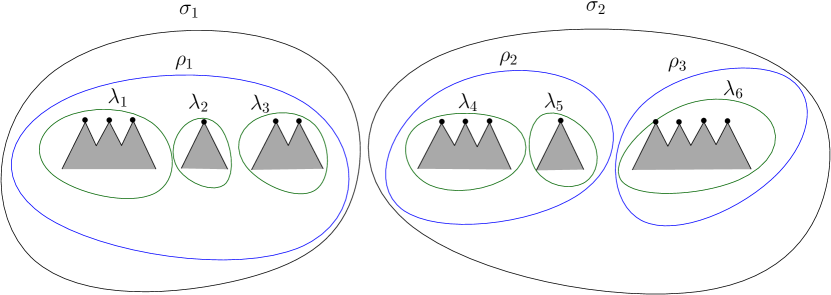
Figure 5: The figure illustrates the nested decomposition $\lambda\hookrightarrow\rho\hookrightarrow\sigma$ in (17.2). The configuration $Z_{n}^{*}$ at time $t$ is represented by $n=14$ black dots. Collision trees, depicted by grey triangles, are created from each dots and all the trees with labels in a subset $\lambda_{i}$ interact via external recollisions, forming connected clusters (grey mountains). These trees are then regrouped in coarser partitions $\rho$ and $\sigma$ in order to evaluate the corresponding cumulants. Green clusters $\lambda$ are called forests, blue clusters $\rho$ are called jungles, and black clusters $\sigma$ are called initial clusters.

Thus we can write

$$F_{n,[0,t]}^{\varepsilon}(H^{\otimes n})=\int dZ_{n}^{*}\!\sum_{\lambda,\rho,\sigma\atop\lambda\hookrightarrow\rho\hookrightarrow\sigma}\int\Big{(}\prod_{i=1}^{\ell}d\mu\big{(}\Psi^{\varepsilon}_{\lambda_{i}}\big{)}\mathcal{H}\big{(}\Psi^{\varepsilon}_{\lambda_{i}}\big{)}\Delta\hskip-5.69046pt\Delta_{\lambda_{i}}\Big{)}\;\varphi_{\rho}\,f^{{\varepsilon}0}_{\sigma}\,.$$ (17.2)

The order of the sums can be exchanged, starting from the coarser partition $\sigma$: we obtain

$$F_{n,[0,t]}^{\varepsilon}(H^{\otimes n})=\int dZ_{n}^{*}\!\sum_{s=1}^{n}\sum_{\sigma\in\mathcal{P}_{n}^{s}}\prod_{j=1}^{s}\!\!\sum_{\lambda,\rho\atop\lambda\hookrightarrow\rho\hookrightarrow\sigma_{j}}\!\int\Big{(}\prod_{i=1}^{\ell}d\mu\big{(}\Psi^{\varepsilon}_{\lambda_{i}}\big{)}\mathcal{H}\big{(}\Psi^{\varepsilon}_{\lambda_{i}}\big{)}\Delta\hskip-5.69046pt\Delta_{\lambda_{i}}\Big{)}\;\varphi_{\rho}f^{{\varepsilon}0}_{\sigma_{j}}$$ (17.3)

where the generic variables $\lambda,\rho$ denote now nested partitions of the subset $\sigma_{j}$.

18 Dynamical cumulants

Using the inversion formula (8.1), the cumulant of order $n$ is defined as the term in (17.3) such that $\sigma$ has only 1 element, i.e. $\sigma=\{1,\dots,n\}$. We therefore define the (scaled) cumulant, recalling notation (17.1),

$${f^{\varepsilon}_{n,[0,t]}(H^{\otimes n})}=\int dZ_{n}^{*}\mu_{\varepsilon}^{n-1}\sum_{\ell=1}^{n}\sum_{\lambda\in\mathcal{P}_{n}^{\ell}}\sum_{r=1}^{\ell}\sum_{\rho\in\mathcal{P}_{\ell}^{r}}\int\Big{(}\prod_{i=1}^{\ell}d\mu\big{(}\Psi^{\varepsilon}_{\lambda_{i}}\big{)}\mathcal{H}\big{(}\Psi^{\varepsilon}_{\lambda_{i}}\big{)}\Delta\hskip-5.69046pt\Delta_{\lambda_{i}}\Big{)}\;\varphi_{\rho}\;f^{{\varepsilon}0}_{\{1,\dots,r\}}(\Psi^{{\varepsilon}0}_{\rho_{1}},\dots,\Psi^{{\varepsilon}0}_{\rho_{r}})\,.$$ (18.1)

In the simple case $n=2$, the above formula reads

$$f_{2,[0,t]}^{\varepsilon}(H^{\otimes 2})=\int dZ_{2}^{*}\,\mu_{\varepsilon}\Big{\{}\int d\mu(\Psi^{\varepsilon}_{\{1,2\}})\,{\bf 1}_{\{1\}\sim_{r}\{2\}}\,\mathcal{H}\big{(}\Psi^{\varepsilon}_{\{1,2\}}\big{)}F^{{\varepsilon}0}(\Psi^{{\varepsilon}0}_{\{1,2\}})$$

$$\quad\;\;-\int\prod_{i=1}^{2}\Big{[}d\mu(\Psi^{\varepsilon}_{\{i\}})\;\mathcal{H}\big{(}\Psi^{\varepsilon}_{\{i\}}\big{)}\Big{]}{\bf 1}_{\{1\}\sim_{o}\{2\}}F^{{\varepsilon}0}\left(\Psi^{{\varepsilon}0}_{\{1\}},\Psi^{{\varepsilon}0}_{\{2\}}\right)$$

$$\quad\;\;+\int\prod_{i=1}^{2}\Big{[}d\mu(\Psi^{\varepsilon}_{\{i\}})\;\mathcal{H}\big{(}\Psi^{\varepsilon}_{\{i\}}\big{)}\Big{]}\left(F^{{\varepsilon}0}\left(\Psi^{{\varepsilon}0}_{\{1\}},\Psi^{{\varepsilon}0}_{\{2\}}\right)-F^{{\varepsilon}0}\left(\Psi^{{\varepsilon}0}_{\{1\}}\right)F^{{\varepsilon}0}\left(\Psi^{{\varepsilon}0}_{\{2\}}\right)\right)\Big{\}},$$

where we used (15.1), (16.3) and (17.1). The three lines on the right hand side represent the three possible correlation mechanisms between particles $1^{*}$ and $2^{*}$ (i.e. between the subtrees $1$ and $2$): respectively the recollision, the overlap and the correlation of initial data.

More generally, looking at Eq. (18.1), we are going to check that ${f^{\varepsilon}_{n,[0,t]}(H^{\otimes n})}$ is a cluster of order $n$, and identify a minimal structure in the spirit as the Penrose partition scheme recalled in Chapter 2.

• We start with $n$ trees which are grouped into $\ell$ forests in the partition $\lambda$. In each forest $\lambda_{i}$ we shall identify $|\lambda_{i}|-1$ “clustering recollisions”. These recollisions give rise to $\sum_{i=1}^{\ell}(|\lambda_{i}|-1)=n-\ell$ constraints.

• The $\ell$ forests are then grouped into $r$ jungles $\rho$ and in each jungle $\rho_{i}$, we shall identify $|\rho_{i}|-1$ “clustering overlaps”. These give rise to $\sum_{i=1}^{r}(|\rho_{i}|-1)=\ell-r$ constraints.

• The $r$ elements of $\rho$ are then coupled by the initial cluster, and this gives rise to $r-1$ constraints.

By construction $n-1=\sum_{i=1}^{r}(|\rho_{i}|-1)+\sum_{i=1}^{\ell}(|\lambda_{i}|-1)+r-1$. The dynamical decomposition (18.1) implies therefore that the cumulant of order $n$ is associated with pseudo-trajectories with $n-1$ clustering constraints, and we expect that each of these $n-1$ clustering constraints will provide a small factor of order $1/\mu_{\varepsilon}$. To quantify rigorously this smallness, we need to identify $n-1$ “independent” degrees of freedom. For clustering overlaps this will be an easy task. Clustering recollisions will require more attention, as they introduce a strong dependence between different trees.

Let us now analyze Eq. (18.1) in more detail. The decomposition can be interpreted in terms of a graph in which the edges represent all possible correlations (between points in a tree, between trees in a forest and between forests in a jungle). In these correlations, some play a special role as they specify minimally connected subgraphs in jungles or forests: this is made precise in the two following important notions.

Let us start with the easier case of overlaps in a jungle. The following definition assigns a minimally connected graph (cf. Definition 9.2) on the set of forests grouped into a given jungle.

Definition 18.1 (Clustering overlaps).

Given a jungle $\rho_{i}=\{\lambda_{j_{1}},\dots,\lambda_{j_{|\rho_{i}|}}\}$ and a pseudo-trajectory $\Psi^{\varepsilon}_{\rho_{i}}$, we call “clustering overlaps” the set of $|\rho_{i}|-1$ overlaps

$$(\lambda_{j_{1}}\sim_{o}\lambda_{j^{\prime}_{1}}),\dots,(\lambda_{j_{|\rho_{i}|-1}}\sim_{o}\lambda_{j^{\prime}_{|\rho_{i}|-1}})$$ (18.2)

such that

$$\Big{\{}\{\lambda_{j_{1}},\lambda_{j^{\prime}_{1}}\},\dots,\{\lambda_{j_{|\rho_{i}|-1}},\lambda_{j^{\prime}_{|\rho_{i}|-1}}\}\Big{\}}=E(T_{\rho_{i}})$$

where $T_{\rho_{i}}$ is the minimally connected graph on $\rho_{i}$ constructed via the Penrose algorithm. Given a pseudo-trajectory $\Psi^{\varepsilon}_{\rho_{i}}$ with clustering overlaps, we define $|\rho_{i}|-1$ overlap times as follows: the $k$-th overlap time is

$$\tau_{{\rm{ov}},k}:=\sup\Big{\{}\tau\geq 0\;:\,\min_{\begin{subarray}{c}\mbox{\tiny$q$ {\rm in} $\Psi^{\varepsilon}_{\lambda_{j_{k}}}$}\\ \mbox{\tiny$q^{\prime}$ {\rm in} $\Psi^{\varepsilon}_{\lambda_{j_{k}^{\prime}}}$}\end{subarray}}|x_{q^{\prime}}(\tau)-x_{q}(\tau)|<{\varepsilon}\Big{\}}\;.$$ (18.3)

Remark 18.2.

Contrary to the case of clustering recollisions defined below (Definition 18.3), there is no privileged way of extracting this minimally connected graph, so we choose the Penrose algorithm (see the proof of Proposition 9.1) for simplicity. Remark that the times $\tau_{{\rm{ov}},k}$ are not ordered.

Each one of the $|\rho_{i}|-1$ overlaps is a strong geometrical constraint which will be used in Part III to gain a small factor $t/\mu_{\varepsilon}$. More precisely, in Chapter 8 we assign to each forest $\lambda_{j_{k}}$ a root $z^{*}_{\lambda_{j_{k}}}$ (chosen among the roots of $\Psi^{\varepsilon}_{\lambda_{j_{k}}}$). Then, it will be possible to “move rigidly” the whole pseudo-trajectory $\Psi^{\varepsilon}_{\lambda_{j_{k}}}$, acting just on $x^{*}_{\lambda_{j_{k}}}$. It follows that one easily translates the condition of “clustering overlap” into $|\rho_{i}|-1$ independent constraints on the relative positions of the roots. In fact remember that the pseudo-trajectories $\Psi^{\varepsilon}_{\lambda_{j_{k}}},\Psi^{\varepsilon}_{\lambda_{j^{\prime}_{k}}}$ do not interact with each other by construction. Therefore $\lambda_{j_{k}}\sim_{o}\lambda_{j^{\prime}_{k}}$ means that the two pseudo-trajectories meet at some time $\tau_{{\rm{ov}},k}>0$ and, immediately after (going backwards), they cross each other freely. This corresponds to a small measure set in the variable $x^{*}_{\lambda_{j_{k}^{\prime}}}-x^{*}_{\lambda_{j_{k}}}$.

Contrary to overlaps, recollisions are unfortunately not independent from one another. For this reason, the study of recollisions of trees in a forest needs more care. In this case we need to fix the order of the recollision times. Then we can identify an ordered sequence of relative positions (between trees) which do not affect the previous recollisions. One by one and following the ordering, such degrees of freedom are shown to belong to a small measure set. The precise identification of degrees of freedom will be explained in Section 32 and is based on the following notion.

Definition 18.3 (Clustering recollisions).

Given a forest $\lambda_{i}=\{i_{1},\dots,i_{|\lambda_{i}|}\}$ and a pseudo-trajectory $\Psi^{\varepsilon}_{\lambda_{i}}$, we call “clustering recollisions” the set of recollisions identified by the following iterative procedure.

- The first clustering recollision is the first external recollision in $\Psi^{\varepsilon}_{\lambda_{i}}$ (going backward in time); we rename the recolliding trees $j_{1},j^{\prime}_{1}$ and the recollision time $\tau_{\rm{rec},1}$.

- The $k$-th clustering recollision is the first external recollision in $\Psi^{\varepsilon}_{\lambda_{i}}$ (going backward in time) such that, calling $j_{k},j^{\prime}_{k}$ the recolliding trees, $\{\{j_{1},j^{\prime}_{1}\},\dots,\{j_{k},j^{\prime}_{k}\}\}=E\left(G^{(k)}\right)$ where $G^{(k)}$ is a graph with no cycles (and no multiple edges). We denote the recollision time $\tau_{\rm{rec},k}$.

In particular,

$$\tau_{\rm{rec},1}\geq\dots\geq\tau_{\rm{rec},|\lambda_{i}|-1}\quad\mbox{and}\quad\Big{\{}\{j_{1},j^{\prime}_{1}\},\dots,\{j_{|\lambda_{i}|-1},j^{\prime}_{|\lambda_{i}|-1}\}\Big{\}}=E(T_{\lambda_{i}})$$ (18.4)

where $T_{\lambda_{i}}$ is a minimally connected graph on $\lambda_{i}$.

If $q,q^{\prime}$ are the particles realizing the $k$-th recollision, we define the corresponding recollision vector by

$$\omega_{\rm{rec},k}:=\frac{x_{q^{\prime}}(\tau_{\rm{rec},k})-x_{q}(\tau_{\rm{rec},k})}{{\varepsilon}}\;.$$ (18.5)

The important difference between Definition 18.3 and Definition 18.1 is that we have given an order to the recollision times in Eq. (18.4) (which does not exist in Eq. (18.3)).

From now on, in order to distinguish, at the level of graphs, between clustering recollisions and clustering overlaps, we shall decorate edges as follows.

Definition 18.4 (Edge sign).

An edge has sign $+$ if it represents a clustering recollision. An edge has sign $-$ if it represents a clustering overlap.

Collecting together clustering recollisions and clustering overlaps, we obtain $r$ minimally connected clusters, one for each jungle. In particular, we can construct a graph $G_{\lambda,\rho}$ made of $r$ minimally connected components. To each $e\in E(G_{\lambda,\rho})$, we associate a sign (+ for a recollision and $-$ for an overlap), and a clustering time $\tau^{clust}_{e}$.

Our main results describing the structure of dynamical correlations will be proved in the third part of this paper. The major breakthrough in this work is to remark that one can obtain uniform bounds for the cumulant of order $n$ for all $n$ with a controlled growth. We recall indeed that we expect each clustering to produce a small factor $t/\mu_{\varepsilon}$, so that the (scaled) cumulant $f^{\varepsilon}_{n}(t)$ of order $n$ defined in (18.1) should be bounded in ${\varepsilon}$. Moreover the number of minimally connected graphs with $n$ vertices is $n^{n-2}$ so we expect $f^{\varepsilon}_{n}(t)$ to grow as $(Ct)^{n-1}n!$. This is made precise in the following theorem, which provides in particular sharp controls on the cumulant generating function $\Lambda^{\varepsilon}_{[0,t]}$ from which the large deviation estimates are derived in Chapter 7. The following theorem will be proved in Section 33 as Theorem 10.

Theorem 4.

Consider the system of hard spheres under the initial measure (1.6), with $f^{0}$ satisfying (1.5). Let $H:D([0,\infty[)\mapsto{\mathbb{R}}$ be a continuous function such that

$$|H^{\otimes n}(Z_{n}([0,t]))|\leq\exp\Big{(}\alpha\,n+\frac{\beta_{0}}{4}\sup_{s\in[0,t]}|V_{n}(s)|^{2}\Big{)}$$ (18.6)

for some $\alpha\in\mathbb{R}$. Define the scaled cumulant ${f^{\varepsilon}_{n,[0,t]}(H^{\otimes n})}$ by (18.1), with the notation (14.5). Then there exists a positive constant $C$ such that the following uniform a priori bound holds for any $t\leq T_{0}$:

$$|{f^{\varepsilon}_{n,[0,t]}(H^{\otimes n})}|\leq(Ce^{\alpha})^{n}\big{(}t+{\varepsilon}\big{)}^{n-1}n!\;.$$ (18.7)

In particular there is a constant $c<1$ depending only on the dimension such that setting $H=e^{h}-1$, the series defining the cumulant generating function is absolutely convergent on a time $[0,T_{\alpha}]$ with $T_{\alpha}=c\,e^{-\alpha}\beta_{0}^{(d+1)/2}/C_{0}$:

$$\forall t\leq T_{\alpha}\,,\quad\Lambda^{\varepsilon}_{[0,t]}(e^{h}):=\frac{1}{\mu_{\varepsilon}}\log{\mathbb{E}}_{\varepsilon}\left(\exp\Big{(}\sum_{i=1}^{\mathcal{N}}h\big{(}{\bf z}^{\varepsilon}_{i}([0,t]\big{)}\Big{)}\right)=\sum_{n=1}^{\infty}{1\over n!}f^{\varepsilon}_{n,[0,t]}\big{(}(e^{h}-1)^{\otimes n}\big{)}\,.$$ (18.8)

Note that (18.8) follows easily from the uniform bounds (18.7) on the rescaled cumulants, recalling Proposition 7.3.

In the next chapter, we shall prove the existence of the limiting cumulant generating function (Theorem 5) and the form of the limit will be characterized explicitly (Theorem 6). As is known from the general theory [DV, dembozeitouni, RezLect] such a result implies upper and lower large deviation bounds, which will be obtained later on in Chapter 7 (see Sections 30.1 and 30.2).

Chapitre 5 Characterization of the limiting cumulants

Thanks to the uniform bounds obtained in Theorem 4 we expect that, for all $n$, there is a limit ${f_{n,[0,t]}(H^{\otimes n})}$ for ${f^{\varepsilon}_{n,[0,t]}(H^{\otimes n})}$ as $\mu_{\varepsilon}\to\infty$. Our goal in this chapter is first to obtain a description of ${f_{n,[0,t]}(H^{\otimes n})}$ in terms of a series expansion similar to (18.1), with a precise definition of the limiting pseudo-trajectories (see Theorem 5 in Section 19 below): the main feature of those pseudo-trajectories is that they correspond to minimally connected collision graphs.

In Section 20 we derive a series expansion for the limiting cumulant generating function (Theorem 6) which is shown to satisfy a Hamilton-Jacobi equation in Section 21 (Theorem 7); the fact that the limiting graphs have no cycles is crucial for the derivation of this equation.

This Hamilton-Jacobi equation encodes all the dynamical correlations. In particular, the convergence of the typical density to the Boltzmann equation is recovered from the Hamilton-Jacobi equation in Section 22 and the limit covariance in Section 23.

19 Limiting pseudo-trajectories and graphical representation of limiting cumulants

In this section we characterize the limiting cumulants ${f_{n,[0,t]}(H^{\otimes n})}$ by their integral representation. This means that we have to specify both the limiting pseudo-trajectories and the limiting measure.

We first describe the formal limit of (18.1). To this end, we start by giving a definition of minimal pseudo-trajectories associated with cumulants for fixed ${\varepsilon}$. Recall that the cumulant ${f^{\varepsilon}_{n,[0,t]}(H^{\otimes n})}$ of order $n$ corresponds to graphs of size $n$ which are completely connected, either by recollisions, or by overlaps, or by initial correlations. It will be proved in Chapter 9 that

• clusterings coming from the defect of factorization of the initial data are smaller by a factor $O({\varepsilon})$ and thus will not contribute to the limit,

• cycles are created by additional (non clustering) recollisions or overlaps and have a vanishing contribution in the limit.

Thus only pseudo-trajectories corresponding to minimally connected graphs will be considered in this section.

Definition 19.1 (Minimal cumulant pseudo-trajectories).

Let $m\geq 0$. The cumulant pseudo-trajectory $\Psi^{\varepsilon}_{n,m}$ associated with the minimally connected graph $T\in\mathcal{T}_{n}^{\pm}$ decorated with edge signs $\left(s^{\rm clust}_{e}\right)_{e\in E(T)}$, and the decorated collision tree $a\in\mathcal{A}_{n,m}^{\pm}$ is obtained by fixing $Z_{n}^{*}$ and a collection of $m$ creation times $T_{m}$ in decreasing order, and parameters $(\Omega_{m},V_{m})$. The cumulant pseudo-trajectory is constructed backward according to the following rules. At each step the set of particles follows the backward free transport until two of them approach at a distance ${\varepsilon}$ or we reach a time $t_{k}$.

At a time $t_{k}$, a new particle, labeled $k$, is adjoined at position $x_{a_{k}}(t_{k})+s_{k}{\varepsilon}\omega_{k}$ and with velocity $v_{k}$.

• If $s_{k}>0$ then the velocities $v_{k}$ and $v_{a_{k}}$ are changed to $v_{k}(t_{k}^{-})$ and $v_{a_{k}}(t_{k}^{-})$ according to the laws (13.1),

• then all particles are transported (backwards) in $\mathcal{D}^{\varepsilon}_{n+k}$.

When two particles, say $\{q_{e},q_{e}^{\prime}\}$, touch, we look at the roots $j$ and $j^{\prime}$ of their respective subtrees.

• If $e=\{j,j^{\prime}\}$ is not an edge of $T$ or if this edge has already appeared before in the (backward) process, then the pseudo-trajectory is not admissible.

• Else we have a clustering recollision if $s^{\rm clust}_{e}=+$ or a clustering overlap if $s^{\rm clust}_{e}=-$. We say that $\{q_{e},q_{e}^{\prime}\}$ is a representative of the edge $e$, and we denote this by $\{q_{e},q_{e}^{\prime}\}\approx e$. The clustering time is denoted $\tau_{e}^{\rm clust}$, and the clustering angle can be defined by

  $$\omega^{\rm clust}_{e}:=\frac{x_{q_{e}}(\tau^{\rm clust}_{e})-x_{q_{e}^{\prime}}(\tau^{\rm clust}_{e})}{{\varepsilon}}\in{\mathbb{S}}^{d-1}\,.$$

The pseudo-trajectory is admissible if at time 0 all edges of $T$ have appeared in the construction. We will order the clustering times, and the edges of $T$ accordingly, and we will denote by $(\Theta^{\rm clust}_{n-1},\Omega^{\rm clust}_{n-1})$ the collection of clustering times and angles.

Theorem 4 will be proved in Section 33 by establishing, in particular, the uniform convergence of the series expansion (18.1) (on the number of created particles $m$, see (14.5)). We thus focus here on a fixed $m$ and a fixed tree $a\in\mathcal{A}^{\pm}_{n,m}$.

The clustering constraints provide $n-1$ conditions on the roots $(z_{i}^{*})_{1\leq i\leq n}$ of the trees, so only one root will be free. We set this root to be $z_{n}^{*}$. Given $(x_{i}^{*},v_{i}^{*})$ and $v_{j}^{*}$ as well as collision parameters $(a,T_{m},\Omega_{m},V_{m})$, since the trajectories are piecewise affine one can perform the local change of variables

$$x_{j}^{*}\in{\mathbb{T}}^{d}\mapsto(\tau^{\rm clust}_{e},\omega^{\rm clust}_{e})\in(0,t)\times{\mathbb{S}}^{d-1}$$ (19.1)

with Jacobian $\mu_{\varepsilon}^{-1}\big{(}(v_{q_{e}}(\tau^{\rm clust+}_{e})-v_{q^{\prime}_{e}}(\tau^{\rm clust+}_{e}))\cdot\omega^{\rm clust}_{e}\big{)}_{+}\,.$ This provides the identification of measures

$$\mu_{\varepsilon}dx_{i}^{*}dv_{i}^{*}dx_{j}^{*}dv_{j}^{*}\\ =dx_{i}^{*}dv_{i}^{*}dv_{j}^{*}d\tau^{\rm clust}_{e}d\omega^{\rm clust}_{e}\big{(}(v_{q_{e}}(\tau^{\rm clust}_{e})-v_{q_{e}^{\prime}}(\tau^{\rm clust}_{e}))\cdot\omega^{\rm clust}_{e}\big{)}_{+}\,.$$ (19.2)

We shall explain in Section 32 how to identify a good sequence of roots to perform this change of variables iteratively (see Figure 6).

Figure 6: On the left figure, two trees (with roots $x_{i}^{*},x_{j}^{*}$) are built independently in the time interval $[\tau_{e},t]$ and their roots are not fixed a priori. On the right figure, the clustering condition at time $\tau_{e}$ imposes a constraint on the relative position $x_{i}^{*}-x_{j}^{*}$ of the roots : the trees are shifted rigidly to satisfy the clustering. This procedure is applied iteratively to determine all relative positions at time $t$. Only one root, say $x_{n}^{*}$, has to be prescribed.

For each tree $a\in\mathcal{A}^{\pm}_{n,m}$, and each minimally connected graph $T\in\mathcal{T}_{n}^{\pm}$, the cumulant pseudo-trajectories are then reparametrized by the root $x_{n}^{*}$, the velocities $V_{n}^{*}$ at time $t$, the sequence $(q_{e},q^{\prime}_{e})_{e\in E(T)}$ of clustering particles, the clustering parameters $(\Theta_{n-1}^{\rm clust},\Omega_{n-1}^{\rm clust})$ and the collision parameters $(T_{m},\Omega_{m},V_{m})$.

Now let us introduce the limiting cumulant pseudo-trajectories and measure.

Definition 19.2 (Limiting cumulant pseudo-trajectories).

Let $m\geq 0$. The limiting cumulant pseudo-trajectories $\Psi_{n,m}$ associated with the ordered trees $T\in\mathcal{T}_{n}^{\pm}$ and $a\in\mathcal{A}_{n,m}^{\pm}$ are obtained by fixing $x_{n}^{*}$ and $V_{n}^{*}$,

• for each $e\in E(T)$, a representative $\{q_{e},q^{\prime}_{e}\}\approx e$

• a collection of $m$ ordered creation times $T_{m}$, and parameters $(\Omega_{m},V_{m})$

• a collection of clustering times and angles $(\Theta^{\rm clust}_{n-1},\Omega^{\rm clust}_{n-1})$.

At each creation time $t_{k}$, a new particle, labeled $k$, is adjoined at position $x_{a_{k}}(t_{k})$ and with velocity $v_{k}$:

• if $s_{k}=+$, then the velocities $v_{k}$ and $v_{a_{k}}$ are changed to $v_{k}(t_{k}^{-})$ and $v_{a_{k}}(t_{k}^{-})$ according to the laws (13.1),

• then all particles follow the backward free flow until the next creation or clustering time.

At each clustering time $\tau^{\rm clust}_{e}$ the particles $q_{e}$ and $q_{e}^{\prime}$ are at the same position:

• if $s_{e}=+$, then the velocities $v_{q_{e}}$ and $v_{q^{\prime}_{e}}$ are changed according to the scattering rule, with scattering vector $\omega^{\rm clust}_{e}$,

• then all particles follow the backward free flow until the next creation or clustering time.

Note that, in Definition 19.1, positions $X_{n}^{*}$ at time $t$ were fixed and clustering conditions were considered as admissibility constraints, while here the positions $X_{n}^{*}$ at time $t$ are not prescribed: they are determined according to an algorithm devised in Section 32.

We can therefore define the limiting measure, with the notation introduced above:

$$d\mu_{{\rm sing},T,a}\left(\Psi_{n,m}\right) :=dT_{m}d\Omega_{m}dV_{m}dx_{n}^{*}dV_{n}^{*}d\Theta^{\rm clust}_{n-1}d\Omega^{\rm clust}_{n-1}\prod_{i=1}^{m}s_{i}\big{(}(v_{i}-v_{a_{i}}(t_{i})\cdot\omega_{i}\big{)}_{+}$$ (19.3)

$$\qquad\times\prod_{e\in E(T)}\sum_{\{q_{e},q_{e}^{\prime}\}\approx e}s^{\rm{clust}}_{e}\big{(}(v_{q_{e}}(\tau^{\rm clust}_{e})-v_{q_{e}^{\prime}}(\tau^{\rm clust}_{e}))\cdot\omega^{\rm clust}_{e}\big{)}_{+}\,.$$

We stress the fact that this measure is supported on singular pseudo-trajectories, in the sense that the pseudo-particles interact one with the other at distance 0.

Equipped with these notations, we can now state the result that will be proved in Chapter 9.

Theorem 5.

With the previous notation and the assumptions of Theorem 4, for all $t\leq T_{0}$, the cumulant ${f^{\varepsilon}_{n,[0,t]}(H^{\otimes n})}$ converges when $\mu_{\varepsilon}\to\infty$ to ${f_{n,[0,t]}(H^{\otimes n})}$ given by

$$\forall t\leq T_{0}\,,\quad{f_{n,[0,t]}(H^{\otimes n})}=\sum_{T\in\mathcal{T}^{\pm}_{n}}\sum_{m=0}^{\infty}\sum_{a\in\mathcal{A}^{\pm}_{n,m}}\int d\mu_{{{\rm sing},T,a}}(\Psi_{n,m})\,\mathcal{H}\big{(}\Psi_{n,m}\big{)}\left(f^{0}\right)^{\otimes m+n}(\Psi^{0}_{n,m})\,.$$ (19.4)

In particular by Theorem 4 there exists a constant $C>0$ and a time $T_{\alpha}<1/C$ depending only on $\alpha,C_{0},\beta_{0}$ such that

$$\forall t\leq T_{\alpha}\,,\quad|{f_{n,[0,t]}(H^{\otimes n})}|\leq C^{n}t^{n-1}n!\,,$$

and the limiting cumulant generating function (18.8) has the form

$$\forall t\leq T_{\alpha}\,,\quad\Lambda_{[0,t]}(e^{h})=\sum_{n=1}^{\infty}{1\over n!}f_{n,[0,t]}\big{(}(e^{h}-1)^{\otimes n}\big{)}=\lim_{\mu_{\varepsilon}\to\infty}\Lambda^{\varepsilon}_{[0,t]}(e^{h})\,.$$ (19.5)

Recall that the convergence time $T_{0}$, in Theorem 1, of the particle system to the solution $f$ of the Boltzmann equation depends only on $f^{0}$ through $C_{0},\beta_{0}$: as noted in Remark 2.2, there holds $T_{0}\sim C_{0}^{-1}\beta_{0}^{(d+1)/2}$. The parameter $\alpha$ quantifies the size of the deviations from $f$ which can be observed. The time $T_{\alpha}$ is then adjusted accordingly : $T_{\alpha}\sim T_{0}e^{-\alpha}$.

20 Limiting cumulant generating function

The following result provides a graphical expansion of $\Lambda_{[0,t]}(e^{h})$.

Theorem 6.

Under the assumptions of Theorem 4, the limiting cumulant generating function $\Lambda_{[0,t]}$ satisfies for all $t\leq T_{\alpha}$

$$\Lambda_{[0,t]}(e^{h})+1=\sum_{K=1}^{\infty}{1\over K!}\sum_{\tilde{T}\in\mathcal{T}_{K}^{\pm}}\int d\mu_{{\rm sing},\tilde{T}}(\Psi_{K,0})(e^{h})^{\otimes K}(\Psi_{K,0})f^{0\otimes K}(\Psi_{K,0}^{0})\,,$$ (20.1)

where

$$d\mu_{{\rm sing},\tilde{T}} :=dx_{K}^{*}dV_{K}\prod_{e=\{q,q^{\prime}\}\in E(\tilde{T})}s_{e}\big{(}(v_{q}(\tau_{e})-v_{q^{\prime}}(\tau_{e}))\cdot\omega_{e}\big{)}_{+}d\tau_{e}d\omega_{e}\,.$$ (20.2)

Furthermore the series is absolutely convergent for $t\in[0,T_{\alpha}]$ :

$$\int d|\mu_{{\rm sing},\tilde{T}}(\Psi_{K,0})|\,(e^{h})^{\otimes K}(\Psi_{K,0})\,f^{0\otimes K}(\Psi_{K,0}^{0})\leq\big{(}Ct\big{)}^{K-1}\,.$$ (20.3)

Compared to Theorem 5, all dynamical connections are dealt with in a symmetric way, resorting to one connected graph $\tilde{T}\in\mathcal{T}_{K}^{\pm}$, rather than a graph $T\in\mathcal{T}^{\pm}_{n}$ encoding recollisions and overlaps and a tree $a\in\mathcal{A}^{\pm}_{n,m}$ encoding collisions.

Démonstration.

By definition and thanks to Theorem 5,

$$\Lambda_{[0,t]}\left(e^{h}\right)=\sum_{n=1}^{\infty}{1\over n!}\sum_{T\in\mathcal{T}^{\pm}_{n}}\sum_{m=0}^{\infty}\sum_{a\in\mathcal{A}^{\pm}_{n,m}}\int d\mu_{{\rm sing},T,a}(\Psi_{n,m})(e^{h}-1)^{\otimes n}\left(f^{0}\right)^{\otimes(m+n)}\,.$$

Note that the trajectories of particles $i\in\{1,\dots,m\}$ can be extended on the whole interval $[0,t]$ just by transporting $i$ without collision on $[t_{i},t]$ : this is actually the only way to have a set of $m+n$ pseudo-trajectories which is minimally connected (any additional collision would add a non clustering constraint, or require adding new particles). It can therefore be identified to some $\Psi_{m+n,0}$ (see Figure 7).

Let us now fix $K=n+m$ and symmetrize over all arguments :

$$\Lambda_{[0,t]}\left(e^{h}\right) =\sum_{K=1}^{\infty}{1\over K!}\sum_{n=1}^{K}{K!\over n!(K-n)!}(K-n)!\sum_{T\in\mathcal{T}^{\pm}_{n}}\sum_{a\in\mathcal{A}^{\pm}_{n,K-n}}\int d\mu_{{\rm sing},T,a}(\Psi_{n,K-n})(e^{h}-1)^{\otimes n}\left(f^{0}\right)^{\otimes K}$$

$$=\sum_{K=1}^{\infty}{1\over K!}\sum_{n=1}^{K}\sum_{\eta\atop|\eta|=n}\sum_{(\eta^{c})^{\prec}}\sum_{T\in\mathcal{T}^{\pm}_{\eta}}\sum_{a\in\mathcal{A}^{\pm}_{\eta,(\eta^{c})^{\prec}}}\int d\mu_{{\rm sing},T,a}(\Psi_{\eta,(\eta^{c})^{\prec}})(e^{h}-1)^{\otimes\eta}\left(f^{0}\right)^{\otimes K}$$

where $\eta$ stands for a subset of $\{1^{*},\dots,n^{*},1,\dots,K-n\}$ with cardinal $n$; $\eta^{c}$ denotes its complement and $(\eta^{c})^{\prec}$ indicates that we have chosen an order on the set $\eta^{c}$. We denote by $\mathcal{A}^{\pm}_{\eta,(\eta^{c})^{\prec}}$ the set of signed trees with roots $\eta$ and added particles with prescribed order in $(\eta^{c})^{\prec}$.

Note that the combinatorics of collisions $a$ and recollisions or overlaps $T$ (together with the choice of the representatives $\{q_{e},q^{\prime}_{e}\}_{e\in E(T)}$) can be described by a single minimally connected graph $\tilde{T}\in\mathcal{T}^{\pm}_{K}$. In order to apply Fubini’s theorem, we then need to understand the mapping

$$(a,T,\{q_{e},q^{\prime}_{e}\}_{e\in E(T)})\mapsto(\tilde{T},\eta)\,.$$

It is easy to see that this mapping is injective but not surjective. Given a pseudo-trajectory $\Psi_{K,0}$ compatible with $\tilde{T}$ and a set $\eta$ of cardinality $n$, we reconstruct $(a,T,\{q_{e},q^{\prime}_{e}\}_{e\in E(T)})$ as follows. We color in red the $n$ particles belonging to $\eta$ at time $t$, and in blue the $K-n$ other particles. Then we follow the dynamics backward. At each clustering, we apply the following rule

• if the clustering involves one red particle and one blue particle, then it corresponds to a collision in the Duhamel pseudo-trajectory. The corresponding edge of $\tilde{T}$ will be described by $a$. We then change the color of the blue particle to red.

• if the clustering involves two red particles, then it corresponds to a recollision in the Duhamel pseudo-trajectory. The corresponding edge of $\tilde{T}$ is therefore an edge $e\in E(T)$ and the two colliding particles determine the representative $\{q_{e},q^{\prime}_{e}\}$.

• if the clustering involves two blue particles, then the pseudo-trajectory is not admissible for $(\tilde{T},\eta)$, as it is not associated to any $(a,T,\{q_{e},q^{\prime}_{e}\}_{e\in E(T)})$.

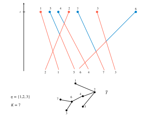
Figure 7: A couple $(\eta,\tilde{T})$ and an associate pseudo-trajectory $\Psi_{K,0}$.

However the contribution of the non admissible pseudo-trajectories $\Psi_{K,0}$ to

$$\sum_{\tilde{T}\in\mathcal{T}_{\eta}^{\pm}}\int d\mu_{{\rm sing},\tilde{T}}(\Psi_{\eta,0})(e^{h})^{\otimes\eta}\left(f^{0}\right)^{\otimes K}$$

is exactly zero. Indeed the blue parts of the trajectories are not weighted, so that the overlap and the recollision terms associated with the first clustering between two blue particles (i.e. the $\pm$ signs of the corresponding edge) exactly compensate.

We therefore conclude that

$$\Lambda_{[0,t]}\left(e^{h}\right) =\sum_{K\geq 1}{1\over K!}\sum_{\tilde{T}\in\mathcal{T}^{\pm}_{K}}\int d\mu_{{\rm sing},\tilde{T}}(\Psi_{K,0})\left(f^{0}\right)^{\otimes K}\sum_{n=1}^{K}\sum_{\eta\in\mathcal{P}^{n}_{K}}(e^{h}-1)^{\otimes\eta}$$

$$=\sum_{K\geq 1}{1\over K!}\sum_{\tilde{T}\in\mathcal{T}^{\pm}_{K}}\int d\mu_{{\rm sing},\tilde{T}}(\Psi_{K,0})(e^{h})^{\otimes K}\left(f^{0}\right)^{\otimes K}-1$$

which is exactly (20.1). Note that the compensation mechanism described above does not work for $n=0$ and $K=1$, which is the reason for the $-1$ in the final formula.

The bound (20.3) comes from the definition of $\mu_{{\rm sing},\tilde{T}}$ together with the estimates used in the proof of Theorem 4 to control the collision cross-sections. ∎

21 Hamilton-Jacobi equations

We consider test functions on the trajectories which write as

$$h(z([0,t]))=g\big{(}t,z(t)\big{)}-\int_{0}^{t}D_{s}g\big{(}s,z(s)\big{)}ds$$ (21.1)

recalling the notation $D_{s}g:=\partial_{s}g+v\cdot\nabla_{x}g$. The effect of this specific choice will be to integrate the transport term in the Hamilton-Jacobi equation. We choose complex-valued functions here as we shall be using properties of analytic functionals of $g$ later; all the results obtained so far can easily be adapted to this more general setting. To stress the dependence on $g$, we introduce a specific notation for the corresponding exponential moment (19.5)

$$\mathcal{I}(t,g):=\Lambda_{[0,t]}(e^{g(t)-\int_{0}^{t}D_{s}g})\,.$$ (21.2)

Note that $g$ is defined here by its final value $g(t)$ and its transport $Dg=(D_{s}g)_{0\leq s\leq t}$, and these two functions will be considered as two independent variables.

The following statement specifies the functional framework in which $\mathcal{I}$ is well defined as a convergent series, and identifies the equation it satisfies. We recall that for any $\alpha\geq 0$, there exists $T_{\alpha}$ (depending only on $\alpha$, $C_{0}$ and $\beta_{0}$) such that the cumulant generating function $\Lambda^{\varepsilon}_{[0,t]}(e^{h})$ is uniformly convergent on $[0,T_{\alpha}]$ provided that $e^{h}-1$ satisfies (18.6). We then define

$${\mathbb{B}}_{\alpha}:=\Big{\{}g\in C^{1}([0,T_{\alpha}]\times\mathbb{D};{\mathbb{C}}) \,:\qquad|g(t,z)|\leq(1-{t\over 2T_{\alpha}})(\alpha+\frac{\beta_{0}}{8}|v|^{2})\,,$$ (21.3)

$$\sup_{s\in[0,T_{\alpha}]}|D_{s}g(s,z)|\leq{1\over 2T_{\alpha}}(\alpha+\frac{\beta_{0}}{8}|v|^{2})\Big{\}}\,.$$

Let us translate Theorems 4 and 6 in terms of the functional $\mathcal{I}$. For $t$ in $[0,T_{\alpha}]$, let $h$ be defined as in (21.1) with $g$ in ${\mathbb{B}}_{\alpha}$. One has

$$\Big{|}\Big{(}e^{h(z_{i}([0,t]))}-1\Big{)}^{\otimes n}\Big{|} \leq e^{\sum_{i=1}^{n}\big{|}h(z_{i}([0,t]))\big{|}}\leq e^{\alpha_{0}n+\frac{\beta_{0}}{8}(1-\frac{t}{2T_{\alpha}})|V_{n}(t)|^{2}+\frac{\beta_{0}}{8}{\frac{1}{2T_{\alpha}}}\int_{0}^{t}|V_{n}(s)|^{2}\,ds}$$ (21.4)

$$\leq e^{\alpha n+\frac{\beta_{0}}{8}\sup_{s\in[0,t]}|V_{n}(s)|^{2}}\,,$$

which is the assumption on $H=e^{h}-1$ of Theorem 4. In particular, the series

$$\mathcal{I}(t,g):=-1+\sum_{K=1}^{\infty}{1\over K!}\sum_{T\in\mathcal{T}_{K}^{\pm}}\int d\mu_{{\rm sing},T}(\Psi_{K,0})(e^{g(t)-\int_{0}^{t}D_{s}g(s)ds})^{\otimes K}(\Psi_{K,0})f^{0\otimes K}(\Psi_{K,0}^{0})$$ (21.5)

is absolutely convergent for $t\in[0,T_{\alpha}]$ and $g\in\mathbb{B}_{\alpha}$. Note that (21.5) shows that $\mathcal{I}$ is analytic with respect to $g(t)$: in particular one can differentiate $\mathcal{I}(t,g)$ with respect to the final condition $g(t)$, in a direction $\Upsilon$ and by term-wise derivation of the series (21.5) we find:

$$\int_{\mathbb{D}}dz{{\partial}\mathcal{I}(t,g)\over{\partial}g(t)}(z)\Upsilon(z) =\sum_{K}{1\over K!}\sum_{\tilde{T}\in\mathcal{T}^{\pm}_{K}}\sum_{i=1}^{K}\int d\mu_{{{\rm sing},\tilde{T}}}(\Psi_{K,0})\Upsilon(z_{i}(t))$$ (21.6)

$$\qquad\qquad\qquad\times\left(e^{g(t)-\int_{0}^{t}D_{s}gds}\right)^{\otimes K}(\Psi_{K,0})\left(f^{0}\right)^{\otimes K}(\Psi^{0}_{K,0})\,.$$

We first state a regularity result on ${{\partial}\mathcal{I}(t,g)\over{\partial}g(t)}$ needed to define the singularity in the Hamilton-Jacobi equation derived in Theorem 7. Additional results on $\mathcal{I}$ in an appropriate functional setting will be derived later in Proposition 29.2 in order to obtain the uniqueness of the Hamilton-Jacobi equation.

Proposition 21.1.

For $t\leq T_{\alpha}$ and $g\in\mathbb{B}_{\alpha}$, the functional derivative $(x,v)\mapsto\displaystyle{{\partial}\mathcal{I}(t,g)\over{\partial}g(t)}(x,v)$ is a continuous function in $x\in\mathbb{T}^{d}$ with values in the space ${\mathcal{M}}_{v}({\mathbb{R}}^{d})$ of weighted measures in $v\in\mathbb{R}^{d}$: there is a constant $C$ such that for any $g\in\mathbb{B}_{\alpha}$,

$$\forall t\leq T_{\alpha}\,,\forall x\in\mathbb{T}^{d},\qquad\Big{\|}{{\partial}\mathcal{I}(t,g)\over{\partial}g(t)}(x,v)\;\exp(\frac{\beta_{0}}{8}|v|^{2})(1+|v|)\Big{\|}_{{\mathcal{M}}_{v}({\mathbb{R}}^{d})}\leq C\,.$$

Démonstration.

Given $K$, we consider the associated integral in the series expansion (21.6). The integrand is uniformly bounded by the assumption (1.5) on $f^{0}$ and inequality (21.4)

$$\Gamma_{K}(\Psi_{K,0}):=\left(e^{g(t)-\int_{0}^{t}D_{s}gds}\right)^{\otimes K}(\Psi_{K,0})\left(f^{0}\right)^{\otimes K}(\Psi^{0}_{K,0})\leq e^{\alpha K-\frac{3\beta_{0}}{8}|V_{K}(0)|^{2}}.$$ (21.7)

The measure $\mu_{{\rm sing},\tilde{T}}$ is invariant under global translations in $x$. Thanks to the upper bound (21.7), each integral in (21.6) is uniformly bounded in terms of $\|\exp(-\frac{\beta_{0}}{8}|v|^{2})(1+|v|)^{-1}\Upsilon\|_{L^{1}_{x}(L^{\infty}_{v})}$

$$\Big{|}\int d\mu_{{{\rm sing},\tilde{T}}}(\Psi_{K,0})\Gamma_{K}(\Psi_{K,0})\Upsilon(z_{i}(t))\Big{|}$$ (21.8)

$$\leq\Big{|}\int d\mu_{{{\rm sing},\tilde{T}}}(\Psi_{K,0})e^{\alpha K-\frac{\beta_{0}}{8}|V_{K}(0)|^{2}}\Big{|}\;\|\exp(-\frac{\beta_{0}}{8}|v|^{2})(1+|v|)^{-1}\Upsilon\|_{L^{1}_{x}(L^{\infty}_{v})}\,.$$

Furthermore, using the continuity of $g$ and $f^{0}$, we deduce that $\Gamma_{K}(\Psi_{K,0})$ is a continuous function of the root $z_{i}(t)$, as changing the position of the root boils down to translating rigidly the whole pseudo-trajectory. Therefore, by density approximation, one can extend the convergence and the bound (21.8) to any $\Upsilon$ such that $\Upsilon\exp(-\frac{\beta_{0}}{8}|v|^{2})(1+|v|)^{-1}\in{\mathcal{M}}_{x}\left(L^{\infty}_{v}\right)$ where ${\mathcal{M}}_{x}$ is the space of measures. Proposition 21.1 is proved by summing the expansion (21.6). ∎

The next theorem is the key to derive the large deviation functional in Chapter 7. As a byproduct, it will also allow us to prove that the limit first cumulant $f_{1}$ solves the Boltzmann equation, and to derive the equation on the limit covariance.

Theorem 7 (Hamilton-Jacobi equation for the limit cumulant generating function).

For any $\alpha>0$, the functional $\mathcal{I}(t,g)$ is well defined on $[0,T_{\alpha}]\times\mathbb{B}_{\alpha}$, and the series defining $\mathcal{I}(t,g)$ is a solution of the mild form of the Hamilton-Jacobi equation on $[0,T_{\alpha}]\times\mathbb{B}_{\alpha}$ :

$$\begin{cases}\mathcal{I}(t,g)&=\displaystyle{\mathcal{I}(0,g)+\frac{1}{2}\int_{0}^{t}d\tau\int{{\partial}\mathcal{I}\over{\partial}g(\tau)}(\tau,g)(z_{1}){{\partial}\mathcal{I}\over{\partial}g(\tau)}(\tau,g)(z_{2})\Big{(}e^{\Delta g(\tau)}-1\Big{)}d\mu(z_{1},z_{2},\omega)}\,,\\ \mathcal{I}(0,g)&=\displaystyle{\int dz\,f^{0}(z)(e^{g(0,z)}-1)}\,,\end{cases}$$ (21.9)

where we used the notation (3.6)-(3.7)

$$d\mu(z_{1},z_{2},\omega):=\delta_{x_{1}-x_{2}}((v_{1}-v_{2})\cdot\omega)_{+}d\omega dv_{1}dv_{2}dx_{1}\,,$$

and

$$\Delta g(z_{1},z_{2},\omega):=g(z^{\prime}_{1})+g(z^{\prime}_{2})-g(z_{1})-g(z_{2})\,.$$

We will see in Chapter 7 that this Hamilton-Jacobi equation provides a complete characterization of $\mathcal{I}$ which will be crucial to identify the large deviation functional by means of Legendre transform.

Démonstration.

At time 0, the exponential moment (21.5) reduces to the exponential moment of independent particles thus only the term $K=1$ remains

$$\mathcal{I}(0,g)=-1+\int dze^{g(0,z)}f^{0}(z)=\int dz\,f^{0}(z)(e^{g(0,z)}-1)\,.$$ (21.10)

To recover the mild form of the Hamilton-Jacobi equation (21.9), we are going to reparametrize each term of the series (21.5) of $\mathcal{I}(t,g)$ by singling out the last clustering collision. Given a tree $T$ in $\mathcal{T}_{K}^{\pm}$ with $K\geq 2$, let $\tau_{e}:=\tau_{e}^{\rm clust}\in[0,t]$ be the last clustering time which occurs at the edge $e$ and is associated with the scattering vector $\omega_{e}:=\omega^{\rm clust}_{e}$ and the sign $s_{e}:=s^{\rm{clust}}_{e}\in\{-1,1\}$. By removing the edge $e$, the tree $T$ is split into two trees $T_{1}\in\mathcal{T}_{K_{1}}^{\pm}$ and $T_{2}\in\mathcal{T}_{K_{2}}^{\pm}$ with sizes $K_{1}+K_{2}=K$ and clustering times belonging to $[0,\tau_{e}]$. These trees generate two pseudo-trajectories $\Psi_{K_{1},0},\Psi_{K_{2},0}$ on $[0,\tau]$ which are then constrained to cluster at time $\tau_{e}$. The whole pseudo-trajectory $\Psi_{K,0}$ on $[0,t]$ (generated by $T$) is then recovered by merging the pseudo-trajectories $\Psi_{K_{1},0},\Psi_{K_{2},0}$ at time $\tau_{e}$ and extending them on $[0,t]$ with a scattering, or not, according to the sign $s_{e}$. This procedure is abbreviated by

$$\Psi_{K,0}=\Psi_{K_{1},0}\wedge\Psi_{K_{2},0}\,.$$ (21.11)

This leads to

$$\sum_{T\in\mathcal{T}_{K}^{\pm}}\int d\mu_{{\rm sing},T}(\Psi_{K,0})(e^{g(t)-\int_{0}^{t}D_{s}g(s)ds})^{\otimes K}(\Psi_{K,0})f^{0\otimes K}(\Psi_{K,0}^{0})$$

$$\quad=\frac{1}{2}\sum_{K_{1},K_{2}\atop K_{1}+K_{2}=K}\frac{K!}{K_{1}!\,K_{2}!}\sum_{T_{1}\in\mathcal{T}_{K_{1}}^{\pm}\atop T_{2}\in\mathcal{T}_{K_{2}}^{\pm}}\int_{0}^{t}d\tau_{e}\int d\mu_{{\rm sing},T_{1}}^{[0,\tau_{e}]}(\Psi_{K_{1},0})d\mu_{{\rm sing},T_{2}}^{[0,\tau_{e}]}(\Psi_{K_{2},0})f^{0\otimes K_{1}}(\Psi_{K_{1},0}^{0})f^{0\otimes K_{2}}(\Psi_{K_{2},0}^{0})$$

$$\qquad\qquad\qquad\times\sum_{i\in T_{1}\atop j\in T_{2}}\sum_{s_{e}=\pm 1}\int d\omega_{e}\;s_{e}\;\delta_{x_{i}(\tau_{e})-x_{j}(\tau_{e})}((v_{i}(\tau_{e}^{-})-v_{j}(\tau_{e}^{-}))\cdot\omega_{e})_{+}\;\ (e^{g(t)-\int_{0}^{t}D_{s}g(s)ds})^{\otimes K},$$ (21.12)

where the edge $e=(i,j)$. By construction the parameters associated with the pseudo-trajectories $\Psi_{K_{1},0}$ and $\Psi_{K_{2},0}$ are independent and the corresponding measures on $[0,\tau_{e}]$ factorize. We used the notation $\mu_{{\rm sing},T_{1}}^{[0,\tau_{e}]}$ to stress the fact that the clustering times of the measure are restricted to $[0,\tau_{e}]$. The last line of the identity (21.12) encodes the clustering constraint at $\tau_{e}$.

To recover the factorization of the Hamilton-Jacobi equation (21.9), we first note that all the particles evolve in straight line in $[\tau_{e},t]$, so that for any $k\leq K$

$$g\big{(}t,z_{k}(t)\big{)}-\int_{0}^{t}D_{s}g\big{(}s,z_{k}(s)\big{)}ds=g\big{(}\tau_{e},z_{k}(\tau_{e}^{+})\big{)}-\int_{0}^{\tau_{e}}D_{s}g\big{(}s,z_{k}(s)\big{)}ds.$$

If $s_{e}=1$, a scattering occurs between the particles $(i,j)$ forming the edge $e$ so that their velocities jump at time $\tau_{e}$; if $s_{e}=-1$ on the other hand, the trajectories are unchanged. With the notation (3.7), the discontinuity at the collision can thus be rewritten as

$$(e^{g(t)-\int_{0}^{t}D_{s}g(s)ds})^{\otimes K} =(e^{g(\tau_{e})-\int_{0}^{\tau_{e}}D_{s}g(s)ds})^{\otimes K_{1}}\;(e^{g(\tau_{e})-\int_{0}^{\tau_{e}}D_{s}g(s)ds})^{\otimes K_{2}}$$

$$\qquad\times\left(1+1_{s_{e}=1}\Big{[}\exp\Big{(}\Delta g(\tau_{e})\;(z_{i}(\tau_{e}^{-}),z_{j}(\tau_{e}^{-}),\omega_{e})\Big{)}-1\Big{]}\right)\,.$$ (21.13)

It follows that except for the interaction at time $\tau_{e}$ between particles $i,j$, the test functions factorize. We can rewrite (21.12) as

$$\sum_{T\in\mathcal{T}_{K}^{\pm}}\int d\mu_{{\rm sing},T}(\Psi_{K,0})(e^{g(t)-\int_{0}^{t}D_{s}g(s)ds})^{\otimes K}(\Psi_{K,0})f^{0\otimes K}(\Psi_{K,0}^{0})$$

$$\quad=\frac{K!}{2}\sum_{K_{1}=0}^{K}\sum_{T_{1}\in\mathcal{T}_{K_{1}}^{\pm}\atop T_{2}\in\mathcal{T}_{K_{2}}^{\pm}}\sum_{i\in T_{1}\atop j\in T_{2}}\int_{0}^{t}d\tau_{e}\prod_{\ell=1,2}\;\left[\frac{1}{K_{\ell}!}\int d\mu_{{\rm sing},T_{\ell}}^{[0,\tau_{e}]}(\Psi_{K_{\ell},0})f^{0\otimes K_{\ell}}(\Psi_{K_{\ell},0}^{0})(e^{g(\tau_{e})-\int_{0}^{\tau_{e}}D_{s}g(s)ds})^{\otimes K_{\ell}}\right]$$

$$\qquad\quad\qquad\times\int d\omega_{e}\;\delta_{x_{i}(\tau_{e})-x_{j}(\tau_{e})}((v_{i}(\tau_{e}^{-})-v_{j}(\tau_{e}^{-}))\cdot\omega_{e})_{+}\;\ \Big{[}\exp\Big{(}\Delta g(\tau_{e})\;(z_{i}(\tau_{e}^{-}),z_{j}(\tau_{e}^{-}),\omega_{e})\Big{)}-1\Big{]},$$ (21.14)

where only the contribution $s_{e}=1$ remains. Indeed the constant $1$ in the last line of (21.13) cancels out after summing over $s_{e}=\pm 1$.

Summing (21.14) over all $K\geq 1$ in order to rebuild $\mathcal{I}(t,g)$, the product of the functional derivatives $\displaystyle{{\partial}\mathcal{I}(\tau_{e},g)\over{\partial}g(\tau_{e})}$ defined in (21.6) can be identified

$$\mathcal{I}(t,g)=\mathcal{I}(0,g)+\frac{1}{2}\int_{0}^{t}d\tau_{e}\int{{\partial}\mathcal{I}\over{\partial}g(\tau_{e})}(\tau_{e},g)(z_{1}){{\partial}\mathcal{I}\over{\partial}g(\tau_{e})}(\tau_{e},g)(z_{2})\Big{(}e^{\Delta g(\tau_{e})}-1\Big{)}d\mu(z_{1},z_{2},\omega_{e}).$$

Theorem 7 is proved. ∎

22 The Boltzmann equation for the limit first cumulant

The Hamilton-Jacobi equation (21.9) encodes all the limiting correlations of the microscopic dynamics. As a first consequence, we are going to recover the convergence of the density to the solution of the Boltzmann equation already stated in Theorem 1.

Let us denote t the backward transport operator by $S_{t}\phi(x,v):=\phi(x-tv,v)$, for any test function $\phi$.

Proposition 22.1.

In the Boltzmann-Grad limit, the rescaled one-particle density converges in the time interval $[0,T_{0}]$ in the sense of measures

$$\lim_{\mu_{\varepsilon}\to\infty}F^{\varepsilon}_{1}(t)=f_{1}(t)=\frac{\partial\mathcal{I}(t,0)}{\partial g(t)}\,\cdotp$$ (22.1)

The limit $f_{1}$ is a mild solution of the Boltzmann equation in a weak form

$$\int_{\mathbb{D}}f_{1}(t,z)\psi(z)\,dz=\int_{\mathbb{D}}S_{t}f^{0}(z)\psi(z)\,dz$$ (22.2)

$$\qquad+\int_{0}^{t}ds\int S_{t-s}\big{(}f_{1}(s,z^{\prime}_{1})f_{1}(s,z^{\prime}_{2})-f_{1}(s,z_{1})f_{1}(s,z_{2})\big{)}\psi(z_{1})\,d\mu(z_{1},z_{2},\omega)\,,$$

for any continuous bounded test function $\psi$.

Démonstration.

We will consider only functional derivatives of $\mathcal{I}$ at $g=0$, thus $\alpha$ can be chosen arbitrarily small so that all the equations obtained from Theorem 7 are valid up to the time $T_{0}=T_{\alpha\big{|}\alpha=0}$.

By definition (21.2) of $\mathcal{I}$

$$\mathcal{I}(t,g)=\sum_{n=1}^{\infty}\frac{1}{n!}f_{n,[0,t]}\Big{(}\big{(}e^{h}-1\big{)}^{\otimes n}\Big{)}\quad\text{with}\quad h\big{(}z([0,t])\big{)}=g(t,z(t))-\int_{0}^{t}D_{s}g(s,z(s))\,ds\,,$$ (22.3)

is a uniformly convergent series for $t\leq T_{\alpha}$ and in particular it is analytic with respect to $g(t)$ for $g$ in $\mathbb{B}_{\alpha}$. Given a test function $\psi$ defined on $\mathbb{D}$ (and acting at time $t$), the derivative at $g=0$ is given by

$$\Big{\langle}\frac{\partial\mathcal{I}(t,0)}{\partial g(t)},\psi\Big{\rangle}=f_{1,[0,t]}(\psi)=\int_{\mathbb{D}}f_{1}(t)\psi(z)\,dz\,,$$ (22.4)

where $\langle\,\cdot\,,\,\cdot\,\rangle$ denotes the duality bracket. Theorem 5 implies that $f^{\varepsilon}_{1,[0,t]}$ converges to $f_{1,[0,t]}$. As $F^{\varepsilon}_{1}(t)=f^{\varepsilon}_{1}(t)$, this leads to (22.1).

The Hamilton-Jacobi equation (21.9) will enable us to obtain rather easily that the equation satisfied by $f_{1}$ is the Boltzmann equation. Let us start by computing the derivative with respect to $g(t)$ of $\mathcal{I}(0,g)$. First, we note that for all $s\in[0,t]$, then $g(s)$ is a function of $g(t)$ and $Dg$ through the Duhamel formula

$$g(t,x+tv,v)=g(s,x+sv,v)+\int_{s}^{t}D_{\sigma}g(\sigma,x+\sigma v,v)\,d\sigma\,,$$

which may be recast as follows:

$$\forall s\in[0,t]\,,\quad g(s)=S_{s-t}g(t)-\int_{s}^{t}S_{s-\sigma}D_{\sigma}g(\sigma)\,d\sigma\,.$$ (22.5)

This formula will be key to track the impact of the variations of $g(s)$ in the functional derivatives under a perturbation of $g$ at time $t$ (or of $Dg$ later on). Recalling that

$$\mathcal{I}(0,g)=\int f^{0}(z)\big{(}e^{g(0,z)}-1\big{)}\,dz\,,$$

we therefore find that taking the derivative with respect to $g(t)$ in the direction $\psi$ is given by

$$\langle\frac{\partial\mathcal{I}(0,g)}{\partial g(t)},\psi\rangle=\int f^{0}(z)\big{(}S_{-t}\psi\big{)}(z)e^{g(0,z)}\,dz\,,$$ (22.6)

hence in particular at $g=0$

$$\langle\frac{\partial\mathcal{I}(0,0)}{\partial g(t)},\psi\rangle=\int\big{(}S_{t}f^{0}\big{)}(z)\psi(z)\,dz\,.$$ (22.7)

Next differentiating (21.9) with respect to $g(t)$ in the direction $\psi$, we find

$$\langle\frac{\partial\mathcal{I}(t,g)}{\partial g(t)},\psi\rangle =\int\big{(}S_{t}f^{0}\big{)}(z)\psi(z)\,dz$$ (22.8)

$$+\int_{0}^{t}ds\int{{\partial}\mathcal{I}(s,g)\over{\partial}g(s)}(z_{1})\Big{\langle}{{\partial}^{2}\mathcal{I}(s,g)\over{\partial}g(s){\partial}g(t)},\psi\Big{\rangle}(z_{2})\Big{(}e^{\Delta g(s)}-1\Big{)}d\mu(z_{1},z_{2},\omega)$$

$$+\frac{1}{2}\int_{0}^{t}ds\int{{\partial}\mathcal{I}(s,g)\over{\partial}g(s)}(z_{1}){{\partial}\mathcal{I}(s,g)\over{\partial}g(s)}(z_{2})\;\Delta S_{s-t}\psi\,e^{\Delta g(s)}d\mu(z_{1},z_{2},\omega).$$

Note that Proposition 21.1 allows to handle the singularity of the measure $d\mu$.

Evaluating the result at $g=0$ produces, thanks to (22.4), (22.5) and (22.7),

$$\langle\frac{\partial\mathcal{I}(t,0)}{\partial g(t)},\psi\rangle=\int\big{(}S_{t}f^{0}\big{)}(z)\psi(z)\,dz+\frac{1}{2}\int_{0}^{t}ds\int f_{1}(s,z_{1})f_{1}(s,z_{2})\Delta S_{s-t}\psi\,d\mu(z_{1},z_{2},\omega)\,.$$

Finally thanks to (22.4) again, we recover that for any smooth function $\psi$

$$\langle f_{1}(t),\psi\rangle =\int\big{(}S_{t}f^{0}\big{)}(z)\psi(z)\,dz+\int_{0}^{t}ds\int\big{(}f_{1}(s,z^{\prime}_{1})f_{1}(s,z^{\prime}_{2})-f_{1}(s,z_{1})f_{1}(s,z_{2})\big{)}S_{s-t}\psi\,d\mu(z_{1},z_{2},\omega)$$

$$=\int\big{(}S_{t}f^{0}\big{)}(z)\psi(z)\,dz+\int_{0}^{t}ds\int S_{t-s}\big{(}f_{1}(s,z^{\prime}_{1})f_{1}(s,z^{\prime}_{2})-f_{1}(s,z_{1})f_{1}(s,z_{2})\big{)}\psi(z_{1})\,d\mu(z_{1},z_{2},\omega).$$

The proposition is proved. ∎

23 Equation for the limit covariance

The fluctuation field covariance is defined for any test functions $\psi,\varphi$ on $\mathbb{D}$ by

$$\forall s\leq t\,,\qquad\mathcal{C}_{\varepsilon}(t,s,\psi,\varphi):={\mathbb{E}}_{\varepsilon}\left(\zeta^{\varepsilon}_{t}(\psi)\zeta^{\varepsilon}_{s}(\varphi)\right).$$ (23.1)

The Hamilton-Jacobi equation (21.9) enables us to deduce dynamical equations characterizing the limit covariance. For this, we shall need the following notations :

Definition 23.1.

The (adjoint) linearized operator is defined as

$$\mathcal{L}_{t}^{*}\varphi(z) :=v\cdot\nabla_{x}\varphi(z)+{\mathbf{L}}_{t}^{*}\varphi(z)\,,\quad\mbox{with}$$ (23.2)

$${\mathbf{L}}_{t}^{*}\varphi(z) :=\int d\mu_{z}(z_{2},\omega)f(t,z_{2})\,\Delta\varphi(z,z_{2},\omega)\,,$$

with notation (2.2) for the measure $d\mu_{z}(z_{2},\omega)$. We also set

$${\bf Cov}_{t}(\varphi,\psi):=\frac{1}{2}\int d\mu(z_{1},z_{2},\omega)\,f(t,z_{1})\,f(t,z_{2})\;\Delta\psi\Delta\varphi\,.$$ (23.3)

Proposition 23.2.

The covariance of the particle system converges to a quadratic form $\mathcal{C}$ in the time interval $[0,T_{0}]$ in a weak sense, i.e. for any bounded continuous functions $\varphi,\psi$

$$\forall s\leq t\leq T_{0},\qquad\lim_{\mu_{\varepsilon}\to\infty}\mathcal{C}_{\varepsilon}(t,s,\psi,\varphi)=\mathcal{C}(t,s,\psi,\varphi)\,.$$ (23.4)

The limit $\mathcal{C}$ is a solution of the system of equations for $t\leq T_{0}$

$$\left\{\begin{aligned} \mathcal{C}(t,t,\psi,\varphi)&=\mathcal{C}(0,0,S_{-t}\psi,S_{-t}\varphi)+\int_{0}^{t}ds\,{\bf Cov}_{s}(S_{s-t}\psi,S_{s-t}\varphi)\\ &+\int_{0}^{t}ds\,\mathcal{C}(s,s,S_{s-t}\psi,{\mathbf{L}}_{s}^{*}S_{s-t}\varphi)+\int_{0}^{t}ds\,\mathcal{C}(s,s,{\mathbf{L}}_{s}^{*}S_{s-t}\psi,S_{s-t}\varphi)\,,\\ \int_{0}^{t}\mathcal{C}(t,\sigma,\psi,\phi_{\sigma})\,d\sigma&=\int_{0}^{t}d\sigma\,\left(\mathcal{C}(\sigma,\sigma,S_{\sigma-t}\psi,\phi_{\sigma})+\int_{\sigma}^{t}ds\;\mathcal{C}\Big{(}s,\sigma,{\mathbf{L}}_{s}^{*}S_{s-t}\psi,\phi_{\sigma}\Big{)}\right)\,,\end{aligned}\right.$$ (23.5)

where $\psi$, $\varphi$ and $(\phi_{\sigma})_{\sigma\leq T_{0}}$ are test functions on $\mathbb{D}$.

It is shown in the appendix that (23.5) provides a complete characterization of $\mathcal{C}(t,s,\psi,\varphi)$, at least for a short time: see Proposition 10.C.1.

Démonstration.

The proof of the proposition is split into 2 steps.

Step 1. Convergence of the covariance (23.4).

Recall first that the covariance, for fixed ${\varepsilon}$, is determined by the first two cumulants

$$\forall s\leq t\,,\quad\mathcal{C}_{\varepsilon}(t,s,\psi,\varphi) ={\mathbb{E}}_{\varepsilon}\left(\frac{1}{\mu_{\varepsilon}}\sum_{i}\varphi({\bf z}^{\varepsilon}_{i}(s))\psi({\bf z}^{\varepsilon}_{i}(t))\right)+{\mathbb{E}}_{\varepsilon}\left(\frac{1}{\mu_{\varepsilon}}\sum_{(i_{1},i_{2})}\varphi({\bf z}^{\varepsilon}_{i_{1}}(s))\psi({\bf z}^{\varepsilon}_{i_{2}}(t))\right)$$

$$\quad-\mu_{\varepsilon}{\mathbb{E}}_{\varepsilon}\left(\frac{1}{\mu_{\varepsilon}}\sum_{i}\varphi({\bf z}^{\varepsilon}_{i}(s))\right)\times{\mathbb{E}}_{\varepsilon}\left(\frac{1}{\mu_{\varepsilon}}\sum_{i}\psi({\bf z}^{\varepsilon}_{i}(t))\right)$$

$$=f^{\varepsilon}_{1,[0,t]}(\varphi(s)\psi(t))+f^{\varepsilon}_{2,[0,t]}(\varphi(s)\otimes\psi(t))$$

where with slight abuse, we denote by $f^{\varepsilon}_{2,[0,t]}=f^{\varepsilon}_{2,[0,t]}\left(\psi\otimes\varphi\right)$ the bilinear form obtained by polarization

$$f^{\varepsilon}_{2,[0,t]}\left(\psi\otimes\varphi\right):=\frac{1}{2}\Big{(}f^{\varepsilon}_{2,[0,t]}\left((\psi+\varphi)^{\otimes 2}\right)-f^{\varepsilon}_{2,[0,t]}\left(\psi^{\otimes 2}\right)-f^{\varepsilon}_{2,[0,t]}\left(\varphi^{\otimes 2}\right)\Big{)}\;.$$

By the convergence of the cumulants proved in Theorem 5, the limit covariance is

$$\forall s\leq t\,,\quad\mathcal{C}(t,s,\psi,\varphi):=f_{1,[0,t]}\big{(}\psi(t)\varphi\big{(}s)\big{)}+f_{2,[0,t]}\big{(}\psi\big{(}t)\otimes\varphi(s)\big{)}\,.$$ (23.6)

Step 2. Derivation of the system of equations (23.5).

We start by establishing the equation for the covariance at a single time $t$. As in (22.4), differentiating twice $\mathcal{I}$ with respect to $g(t)$ in the direction $\psi$ provides

$$\Big{\langle}\frac{\partial^{2}\mathcal{I}}{\partial^{2}g(t)},\psi\otimes\psi\Big{\rangle}_{\big{|}g=0}=f_{1,t}(\psi^{2})+f_{2,t}(\psi\otimes\psi)=\mathcal{C}(t,t,\psi,\psi)\,.$$

The corresponding formula for $\mathcal{C}(t,t,\varphi,\psi)$ follows by polarization. Thanks to (22.6), there holds

$$\Big{\langle}\frac{\partial^{2}\mathcal{I}(0,g)}{\partial^{2}g(t)},\psi\otimes\psi\Big{\rangle}_{\big{|}g=0}=\int f^{0}(z)\big{(}S_{-t}\psi\big{)}^{2}(z)\,dz=\mathcal{C}(0,0,S_{-t}\psi,S_{-t}\psi)\,.$$

By using the identity (22.5), the functional can be also differentiated at different times

$$\Big{\langle}{{\partial}^{2}\mathcal{I}(s,g)\over{\partial}g(s){\partial}g(t)},\psi\Big{\rangle}(z_{1})=\Big{\langle}{{\partial}^{2}\mathcal{I}(s,g)\over{\partial}g(s){\partial}g(s)},S_{s-t}\psi\Big{\rangle}(z_{1}).$$ (23.7)

Thus differentiating (22.8) one more time and computing the result at $g=0$ provides

$$\mathcal{C}(t,t,\psi,\psi) =\mathcal{C}(0,0,S_{-t}\psi,S_{-t}\psi)$$ (23.8)

$$\quad+2\int_{0}^{t}ds\int\Big{\langle}{{\partial}^{2}\mathcal{I}(s,0)\over{\partial}g(s){\partial}g(s)},S_{s-t}\psi\Big{\rangle}(z_{1})\;{{\partial}\mathcal{I}(s,0)\over{\partial}g(s)}(z_{2})\;\Delta S_{s-t}\psi\,d\mu(z_{1},z_{2},\omega)$$

$$\quad+\frac{1}{2}\int_{0}^{t}ds\int{{\partial}\mathcal{I}(s,0)\over{\partial}g(s)}(z_{1}){{\partial}\mathcal{I}(s,0)\over{\partial}g(s)}(z_{2})\big{(}\Delta S_{s-t}\psi\big{)}^{2}d\mu(z_{1},z_{2},\omega)$$

$$=\mathcal{C}(0,0,S_{-t}\psi,S_{-t}\psi)$$

$$\quad+2\int_{0}^{t}ds\int\Big{\langle}{{\partial}^{2}\mathcal{I}(s,0)\over{\partial}g(s){\partial}g(s)}(z_{1}),S_{s-t}\psi\Big{\rangle}\;f(s,z_{2})\;\Delta S_{s-t}\psi\,d\mu(z_{1},z_{2},\omega)$$

$$\quad+\frac{1}{2}\int_{0}^{t}ds\int f(s,z_{1})f(s,z_{2})\big{(}\Delta S_{s-t}\psi\big{)}^{2}d\mu(z_{1},z_{2},\omega)\,,$$

where $\displaystyle{{\partial}\mathcal{I}(s,0)\over{\partial}g(s)}$ has been replaced by $f(s)$ thanks to Proposition 22.1.

With these notations, (23.8) can be rewritten as

$$\mathcal{C}(t,t,\psi,\psi)=\mathcal{C}(0,0,S_{-t}\psi,S_{-t}\psi)+2\int_{0}^{t}ds\,\mathcal{C}(s,s,S_{s-t}\psi,{\mathbf{L}}_{s}^{*}S_{s-t}\psi)+\int_{0}^{t}ds\,{\bf Cov}_{s}(S_{s-t}\psi,S_{s-t}\psi)\,.$$ (23.9)

Thus the first equation of the system (23.5) is recovered by polarisation.

Now let us turn to the equation on the covariance at two different times. Given $\phi$ a test function defined on $[0,t]\times\mathbb{D}$, the integrated covariance can be recovered by differentiating with respect to $Dg$ in the direction  $\phi_{\sigma}=\phi(\sigma)$, a given smooth function. Setting

$$\Phi(t,z([0,t])):=\int_{0}^{t}\phi(\sigma,z(\sigma))\,d\sigma=\int_{0}^{t}\phi_{\sigma}\,d\sigma\,,$$

one has

$$\langle\frac{\partial^{2}\mathcal{I}(t,0)}{\partial g(t)\partial Dg},\psi\otimes\Phi\rangle=-f_{1,[0,t]}(\psi\,\Phi)-f_{2,[0,t]}(\psi\otimes\Phi)=-\int_{0}^{t}\mathcal{C}(t,s,\psi,\phi_{s})\,ds,$$

where the minus sign comes from the fact that the test function is $g(t)-\displaystyle\int_{0}^{t}dsD_{s}g$.

We are now going to derive the second equation on the covariance at different times, differentiating (22.8) again. We recall from (22.5) that the variations of $g(s)$ in the directions $\psi$ and $\phi$ are given by

$$\forall s\in[0,t]\,,\quad\delta g(s)=S_{s-t}\psi-\int_{s}^{t}S_{s-\sigma}\phi_{\sigma}\,d\sigma.$$ (23.10)

We start by observing that taking a second derivative in (22.6) leads to

$$\Big{\langle}\frac{\partial^{2}\mathcal{I}(0,0)}{\partial g(t)\partial Dg},\psi\otimes\Phi\Big{\rangle}=-\int dzf^{0}(z)S_{-t}\psi(z)\int_{0}^{t}S_{-\sigma}\phi(\sigma,z)d\sigma=-\int_{0}^{t}\mathcal{C}\big{(}0,0,S_{-t}\psi,S_{-\sigma}\phi_{\sigma}\big{)}\,d\sigma.$$

Taking the derivative at intermediate times $s\in[0,t]$ on $\mathcal{I}(s,g)$ with respect to $Dg$ is more delicate as there is a contribution of the variation of $\delta g(s)$ by (23.10) and another contribution accounting for the variations on $[0,s]$: recalling (22.3),

$$\langle\frac{\partial\mathcal{I}(s,0)}{\partial Dg},\Phi\rangle=-\int_{s}^{t}\Big{\langle}\frac{\partial\mathcal{I}(s,0)}{\partial g(s)},S_{s-\sigma}\phi_{\sigma}\Big{\rangle}\,d\sigma-\int_{0}^{s}\Big{\langle}\frac{\partial\mathcal{I}(s,0)}{\partial D_{\sigma}g},\phi_{\sigma}\Big{\rangle}\,d\sigma.$$ (23.11)

Differentiating (22.8) one more time and using (23.7), there holds

$$\int_{0}^{t} \mathcal{C}(t,\sigma,\psi,\phi_{\sigma})\,d\sigma=\int_{0}^{t}\mathcal{C}(0,0,S_{-t}\psi,S_{-\sigma}\phi_{\sigma})\,d\sigma$$

$$\quad+\int_{0}^{t}ds\int\Big{\langle}{{\partial}^{2}\mathcal{I}(s,0)\over{\partial}g(s){\partial}g(s)},S_{s-t}\psi\Big{\rangle}(z_{1})\,{{\partial}\mathcal{I}(s,0)\over{\partial}g(s)}(z_{2})\Big{(}\Delta\int_{s}^{t}S_{s-\sigma}\phi_{\sigma}\,d\sigma\Big{)}\,d\mu(z_{1},z_{2},\omega)$$

$$\quad-\int_{0}^{t}ds\int\langle{{\partial}^{2}\mathcal{I}(s,0)\over{\partial}g(s){\partial}Dg},\Phi\rangle(z_{1})\,{{\partial}\mathcal{I}(s,0)\over{\partial}g(s)}(z_{2})\Delta S_{s-t}\psi\ \,d\mu(z_{1},z_{2},\omega)$$

$$\quad+\frac{1}{2}\int_{0}^{t}ds\int{{\partial}\mathcal{I}(s,0)\over{\partial}g(s)}(z_{1}){{\partial}\mathcal{I}(s,0)\over{\partial}g(s)}(z_{2})\big{(}\Delta S_{s-t}\psi\big{)}\Big{(}\Delta\int_{s}^{t}S_{s-\sigma}\phi_{\sigma}\,d\sigma\Big{)}d\mu(z_{1},z_{2},\omega)\,.$$

Using that ${{\partial}\mathcal{I}(s,0)\over{\partial}g(s)}=f(s)$ by Proposition 22.1, the adjoint linearized operator (23.2) and the covariance (23.3), we get

$$\int_{0}^{t}\mathcal{C}(t,\sigma,\psi,\phi_{\sigma})\,d\sigma =\int_{0}^{t}\mathcal{C}(0,0,S_{-t}\psi,S_{-\sigma}\phi_{\sigma})\,d\sigma+\int_{0}^{t}ds\int_{s}^{t}d\sigma\;\Big{\langle}{{\partial}^{2}\mathcal{I}(s,0)\over{\partial}g(s){\partial}g(s)},S_{s-t}\psi\otimes{\mathbf{L}}_{s}^{*}S_{s-\sigma}\phi_{\sigma}\Big{\rangle}$$

$$-\int_{0}^{t}ds\;\langle{{\partial}^{2}\mathcal{I}(s,0)\over{\partial}g(s){\partial}Dg},{\mathbf{L}}_{s}^{*}S_{s-t}\psi\otimes\Phi\rangle+\int_{0}^{t}ds\int_{s}^{t}d\sigma\;{\bf Cov}_{s}\Big{(}S_{s-t}\psi,S_{s-\sigma}\phi_{\sigma}\Big{)}.$$

From identity (23.11), we finally obtain

$$\int_{0}^{t}\mathcal{C}(t,\sigma,\psi,\phi_{\sigma})\,d\sigma =\int_{0}^{t}\mathcal{C}(0,0,S_{-t}\psi,S_{-\sigma}\phi_{\sigma})\,d\sigma+\int_{0}^{t}ds\int_{s}^{t}d\sigma\;\Big{\langle}{{\partial}^{2}\mathcal{I}(s,0)\over{\partial}g(s){\partial}g(s)},S_{s-t}\psi\otimes{\mathbf{L}}_{s}^{*}S_{s-\sigma}\phi_{\sigma}\Big{\rangle}$$

$$+\int_{0}^{t}ds\int_{s}^{t}d\sigma\Big{\langle}{{\partial}^{2}\mathcal{I}(s,0)\over{\partial}g(s){\partial}g(s)},{\mathbf{L}}_{s}^{*}S_{s-t}\psi\otimes S_{s-\sigma}\phi_{\sigma}\Big{\rangle}$$

$$+\int_{0}^{t}ds\int_{0}^{s}d\sigma\Big{\langle}{{\partial}^{2}\mathcal{I}(s,0)\over{\partial}g(s){\partial}Dg},{\mathbf{L}}_{s}^{*}S_{s-t}\psi\otimes\phi_{\sigma}\Big{\rangle}$$

$$+\int_{0}^{t}ds\int_{s}^{t}d\sigma\;{\bf Cov}_{s}\Big{(}S_{s-t}\psi,S_{s-\sigma}\phi_{\sigma}\Big{)}.$$

Noticing that

$$\mathcal{C}(s,\sigma,\psi,\phi)=\Big{\langle}{{\partial}^{2}\mathcal{I}(s,0)\over{\partial}g(s){\partial}D_{\sigma}g},\psi\otimes\phi\Big{\rangle},$$

this can be rewritten in terms on the covariance $\mathcal{C}$.

$$\int_{0}^{t}\mathcal{C}(t,\sigma,\psi,\phi_{\sigma})\,d\sigma =\int_{0}^{t}d\sigma\,\mathcal{C}(0,0,S_{-t}\psi,S_{-\sigma}\phi_{\sigma})+\int_{0}^{t}ds\int_{s}^{t}d\sigma\;\mathcal{C}\Big{(}s,s,S_{s-t}\psi,{\mathbf{L}}_{s}^{*}S_{s-\sigma}\phi_{\sigma}\Big{)}$$

$$+\int_{0}^{t}ds\int_{s}^{t}d\sigma\;\mathcal{C}\Big{(}s,s,{\mathbf{L}}_{s}^{*}S_{s-t}\psi,S_{s-\sigma}\phi_{\sigma}\Big{)}+\int_{0}^{t}ds\int_{0}^{s}d\sigma\;\mathcal{C}\Big{(}s,\sigma,{\mathbf{L}}_{s}^{*}S_{s-t}\psi,\phi_{\sigma}\Big{)}$$

$$+\int_{0}^{t}ds\int_{s}^{t}d\sigma\;{\bf Cov}_{s}\Big{(}S_{s-t}\psi,S_{s-\sigma}\phi_{\sigma}\Big{)}.$$

Finally swapping the integrals in $s,\sigma$ by Fubini’s Theorem, we get

$$\int_{0}^{t}\mathcal{C}(t,\sigma,\psi,\phi_{\sigma})\,d\sigma =\int_{0}^{t}d\sigma\,\mathcal{C}(0,0,S_{-t}\psi,S_{-\sigma}\phi_{\sigma})+\int_{0}^{t}d\sigma\int_{0}^{\sigma}ds\;\mathcal{C}\Big{(}s,s,S_{s-t}\psi,{\mathbf{L}}_{s}^{*}S_{s-\sigma}\phi_{\sigma}\Big{)}$$

$$+\int_{0}^{t}d\sigma\int_{0}^{\sigma}ds\;\mathcal{C}\Big{(}s,s,{\mathbf{L}}_{s}^{*}S_{s-t}\psi,S_{s-\sigma}\phi_{\sigma}\Big{)}+\int_{0}^{t}d\sigma\int_{\sigma}^{t}ds\;\mathcal{C}\Big{(}s,\sigma,{\mathbf{L}}_{s}^{*}S_{s-t}\psi,\phi_{\sigma}\Big{)}$$

$$+\int_{0}^{t}d\sigma\int_{0}^{\sigma}ds\;{\bf Cov}_{s}\Big{(}S_{s-t}\psi,S_{s-\sigma}\phi_{\sigma}\Big{)}.$$

Noticing that (23.9) implies

$$\mathcal{C}(\sigma,\sigma,S_{\sigma-t}\psi,\phi_{\sigma}) =\mathcal{C}(0,0,S_{-t}\psi,S_{-\sigma}\phi_{\sigma})+\int_{0}^{\sigma}ds\,\mathcal{C}(s,s,S_{s-t}\psi,{\mathbf{L}}_{s}^{*}S_{s-\sigma}\phi_{\sigma})$$

$$+\int_{0}^{\sigma}ds\,\mathcal{C}(s,s,{\mathbf{L}}_{s}^{*}S_{s-t}\psi,S_{s-\sigma}\phi_{\sigma})+\int_{0}^{\sigma}ds\,{\bf Cov}_{s}(S_{s-t}\psi,S_{s-\tau}\phi_{\sigma})\,,$$

the formula for the covariance simplifies

$$\int_{0}^{t}\mathcal{C}(t,\sigma,\psi,\phi_{\sigma})\,d\sigma=\int_{0}^{t}d\sigma\,\left(\mathcal{C}(\sigma,\sigma,S_{\sigma-t}\psi,\phi_{\sigma})+\int_{\sigma}^{t}ds\;\mathcal{C}\Big{(}s,\sigma,{\mathbf{L}}_{s}^{*}S_{s-t}\psi,\phi_{\sigma}\Big{)}\right).$$

This completes the derivation of the system of equations (23.5). ∎

Deuxième partie Fluctuations around the Boltzmann dynamics

Chapitre 6 Fluctuating Boltzmann equation

The goal of this chapter is to prove Theorem 2, describing the limit of the fluctuation field $(\zeta^{\varepsilon}_{t})_{t}$, of which we recall the definition:

$$\zeta^{\varepsilon}_{t}\big{(}\varphi\big{)}:=\frac{1}{\sqrt{\mu_{\varepsilon}}}\Big{(}\sum_{i=1}^{\mathcal{N}}\varphi\big{(}\mathbf{z}^{\varepsilon}_{i}(t)\big{)}-\mu_{\varepsilon}{\mathbb{E}}_{\varepsilon}\big{(}\pi^{\varepsilon}_{t}(\varphi)\big{)}\Big{)}$$

on test functions $\varphi$. Namely we prove that, in the Boltzmann-Grad limit, $\zeta^{\varepsilon}_{t}$ converges to a process $\zeta_{t}$ which solves, in a weak sense clarified below (see Section 24), the fluctuating Boltzmann equation

$$d\hat{\zeta}_{t}=\mathcal{L}_{t}\,\hat{\zeta}_{t}\,dt+d\eta_{t}\,.$$ (23.1)

We recall that $f$ is the solution of the Boltzmann equation on $[0,T_{0}]$, that the linearized Boltzmann operator is defined as $\mathcal{L}_{t}:=-v\cdot\nabla_{x}+{\bf L}_{t}$ with the collision part

$${\bf L}_{t}\,\varphi(z_{1}):=\int d\mu_{z_{1}}(z_{2},\omega)\Big{(}f(t,z_{2}^{\prime})\varphi(z_{1}^{\prime})+f(t,z_{1}^{\prime})\varphi(z_{2}^{\prime})-f(t,z_{2})\varphi(z_{1})-f(t,z_{1})\varphi(z_{2})\Big{)}\,,$$ (23.2)

and that $d\eta_{t}(x,v)$ is a Gaussian noise with zero mean and covariance given in (23.3), which we recall

$${\bf Cov}_{t}(\psi,\varphi):=\frac{1}{2}\int d\mu(z_{1},z_{2},\omega)\,f(t,z_{1})\,f(t,z_{2})\;\Delta\psi\Delta\varphi\,.$$ (23.3)

where the scattering measures are defined as in (3.6) and (2.2)

$$d\mu_{z_{1}}(z_{2},\omega)=\delta_{x_{1}-x_{2}}\big{(}(v_{1}-v_{2})\cdot\omega\big{)}_{+}d\omega dv_{2},$$

$$d\mu(z_{1},z_{2},\omega)=\delta_{x_{1}-x_{2}}\left((v_{1}-v_{2})\cdot\omega\right)_{+}d\omega\,dx_{1}dv_{1}dv_{2}\,,$$

and we recall the notation

$$\Delta\psi(z_{1},z_{2},\omega)=\psi(z_{1}^{\prime})+\psi(z_{2}^{\prime})-\psi(z_{1})-\psi(z_{2})\,.$$ (23.4)

The limiting Gaussian process (23.1) will be characterized by its covariance in Section 24.

In order to obtain the convergence of the fluctuation field, we shall proceed in two steps, establishing first the convergence of the characteristic function in Section 25.1, and then some tightness in Section 25.2.

24 Weak solutions for the limit process

A solution $\hat{\zeta}_{t}$ to (23.1) is a Gaussian process: its law is therefore completely characterized by its covariance. In this section we study the equation governing this covariance

$$\hat{\mathcal{C}}(t,s,\psi,\varphi):={\mathbb{E}}\big{(}\hat{\zeta}_{t}(\psi)\hat{\zeta}_{s}(\varphi)\big{)}$$ (24.1)

and prove that it is precisely the equation obtained Proposition 23.2, namely (23.5). Since there is a unique solution to (23.5) (see Proposition 10.C.1), the limiting covariance $\mathcal{C}(t,s,\psi,\varphi)$ is equal to $\hat{\mathcal{C}}(t,s,\psi,\varphi)$, at least for short times.

24.1 Equation for the covariance

Denote by $\mathcal{U}(t,s)$ the semigroup associated with $\mathcal{L}_{\tau}$ between times $s<t$, meaning that

$${\partial}_{t}\mathcal{U}(t,s)\varphi-\mathcal{L}_{t}\mathcal{U}(t,s)\varphi=0\,,\qquad\mathcal{U}(s,s)\varphi=\varphi\,,$$

and

$${\partial}_{s}\mathcal{U}(t,s)\varphi+\mathcal{U}(t,s)\mathcal{L}_{s}\varphi=0\,,\qquad\mathcal{U}(t,t)\varphi=\varphi\,.$$

By definition, $\mathcal{U}^{*}(t,s)\varphi$ satisfies

$${\partial}_{s}\mathcal{U}^{*}(t,s)\varphi+\mathcal{L}_{s}^{*}\mathcal{U}^{*}(t,s)\varphi=0\,,\qquad\mathcal{U}^{*}(t,t)\varphi=\varphi\,,$$ (24.2)

and

$${\partial}_{t}\mathcal{U}^{*}(t,s)\varphi-\mathcal{U}^{*}(t,s)\mathcal{L}_{t}^{*}\varphi=0\,,\qquad\mathcal{U}^{*}(s,s)\varphi=\varphi\,,$$

where we recall that $\mathcal{L}_{s}^{*}=v\cdot\nabla_{x}+{\bf L}_{s}^{*}$ with

$${\bf L}_{s}^{*}\,\psi(z_{1}):=\int d\mu_{z_{1}}(z_{2},\omega)f(s,z_{2})\,\Delta\psi(z_{1},z_{2},\omega)\,.$$ (24.3)

Formally, a solution of the limit process (23.1) satisfies for any test function $\varphi$

$$\hat{\zeta}_{t}(\varphi)=\zeta_{0}(\mathcal{U}^{*}(t,0)\varphi)+\int_{0}^{t}\,d\eta_{s}(\mathcal{U}^{*}(t,s)\varphi)\,.$$

For any $t\geq s$ and test functions $\varphi,\psi$, the covariance is then given by

$${\mathbb{E}}\big{(}\hat{\zeta}_{t}(\psi)\hat{\zeta}_{s}(\varphi)\big{)} ={\mathbb{E}}\Big{(}\zeta_{0}\big{(}\mathcal{U}^{*}(t,0)\psi\big{)}\;\zeta_{0}\big{(}\mathcal{U}^{*}(s,0)\varphi\big{)}\Big{)}+{\mathbb{E}}\left(\int_{0}^{t}\int_{0}^{s}d\eta_{\sigma}\,d\eta_{\sigma^{\prime}}\big{(}\mathcal{U}^{*}(t,\sigma)\psi\big{)}\big{(}\mathcal{U}^{*}(s,\sigma^{\prime})\varphi\big{)}\right)$$

$$+{\mathbb{E}}\left(\zeta_{0}\big{(}\mathcal{U}^{*}(t,0)\psi\big{)}\;\int_{0}^{s}d\eta_{\sigma^{\prime}}\big{(}\mathcal{U}^{*}(s,\sigma^{\prime})\varphi\big{)}\right)+{\mathbb{E}}\left(\zeta_{0}\big{(}\mathcal{U}^{*}(s,0)\varphi\big{)}\;\int_{0}^{t}d\eta_{\sigma}\big{(}\mathcal{U}^{*}(t,\sigma)\psi\big{)}\right)$$

so that according to (23.3) and (24.1)

$$\hat{\mathcal{C}}(t,s,\psi,\varphi)={\mathbb{E}}\Big{(}\zeta_{0}\big{(}\mathcal{U}^{*}(t,0)\psi\big{)}\;\zeta_{0}\big{(}\mathcal{U}^{*}(s,0)\varphi\big{)}\Big{)}+\int_{0}^{s}d\sigma\;{\bf Cov}_{\sigma}\left(\mathcal{U}^{*}(t,\sigma)\psi,\mathcal{U}^{*}(s,\sigma)\varphi\right)\,.$$ (24.4)

Definition 24.1.

A weak solution to (23.1) is a Gaussian process with covariance satisfying (24.4).

Let us take formally the time derivative of (24.4) for $t>s$. This gives

$$\partial_{t}\hat{\mathcal{C}}(t,s,\psi,\varphi) ={\mathbb{E}}\left(\zeta_{0}\big{(}\mathcal{U}^{*}(t,0)\mathcal{L}_{t}^{*}\psi\big{)}\zeta_{0}\big{(}\mathcal{U}^{*}(s,0)\varphi\big{)}\right)+\int_{0}^{s}\!\!d\sigma{\bf Cov}_{\sigma}\left(\big{(}\mathcal{U}^{*}(t,\sigma)\mathcal{L}_{t}^{*}\psi\big{)},\big{(}\mathcal{U}^{*}(s,\sigma)\varphi\big{)}\right)$$

$$=\hat{\mathcal{C}}(t,s,\mathcal{L}_{t}^{*}\psi,\varphi)\,.$$

For $s=t$, the time derivative is

$$\partial_{t}\hat{\mathcal{C}}(t,t,\psi,\varphi) =\hat{\mathcal{C}}(t,t,\mathcal{L}_{t}^{*}\psi,\varphi)+\hat{\mathcal{C}}(t,t,\psi,\mathcal{L}_{t}^{*}\varphi)+{\bf Cov}_{t}(\psi,\varphi)\,.$$

We recognize here the equation (23.5) satisfied by the limit covariance $\mathcal{C}(s,t,\varphi,\psi)$ (see Proposition 23.2), written in infinitesimal form:

$$\forall s\leq t,\qquad\begin{cases}{\partial}_{t}\mathcal{C}(t,s,\psi,\varphi)=\mathcal{C}(t,s,\mathcal{L}_{t}^{*}\psi,\varphi),\\ {\partial}_{t}\mathcal{C}(t,t,\psi,\varphi)=\mathcal{C}(t,t,\mathcal{L}_{t}^{*}\psi,\varphi)+\mathcal{C}(t,t,\psi,\mathcal{L}_{t}^{*}\varphi)+{\bf Cov}_{t}(\psi,\varphi)\,,\\ \mathcal{C}(0,0,\psi,\varphi)=\displaystyle\int dz\varphi(z)\psi(z)f^{0}(z)\,.\end{cases}$$ (24.5)

The link between (23.5) and (24.4) is made rigorous in Lemma 24.5 below. The set of equations (24.5) is used in the physics literature to describe correlations at equal and unequal times: we refer to [EC81] which includes a comparison of several equivalent formulations of the right-hand side.

Remark 24.2.

The equilibrium case (when $f^{0}=M$ is a Maxwellian) is much simpler. The linear operator $\mathcal{L}_{\rm eq}:=-v\cdot\nabla_{x}+{\bf L}_{\rm eq}$, where ${\bf L}_{\rm eq}$ is the (autonomous) linearized operator around $M$, generates indeed a semigroup $\mathcal{U}_{\rm eq}$ of self-adjoint contractions on $L^{2}(Mdvdx)$. By the method of [holley1978generalized], one can construct a martingale solution of the generalized Ornstein-Uhlenbeck equation

$$d\hat{\zeta}_{t}=\mathcal{L}_{\rm eq}\,\hat{\zeta}_{t}\,dt+d\eta_{t}\;.$$ (24.6)

Moreover, the covariance structure is such that the fluctuations exactly compensate the dissipation : using the symmetry of the equilibrium measure $M(z_{1}^{\prime})M(z_{2}^{\prime})=M(z_{1})M(z_{2})$ and denoting by $\mathcal{U}_{\rm eq}^{*}$ the adjoint of $\mathcal{U}_{\rm eq}$ in $L^{2}(\mathbb{D})$, one gets

$$\int_{0}^{t}du\,{\bf Cov}\big{(}\mathcal{U}_{\rm eq}^{*}(t,\sigma)\varphi,\mathcal{U}_{\rm eq}^{*}(t,\sigma)\varphi\big{)} =-2\int_{0}^{t}d\sigma\int\mathcal{U}_{\rm eq}^{*}(t,\sigma)\varphi M{\bf L}_{\rm eq}^{*}\;\mathcal{U}_{\rm eq}^{*}(t,\sigma)\varphi$$

$$=-2\int_{0}^{t}d\sigma\int\mathcal{U}_{\rm eq}^{*}(t,\sigma)\varphi M(-{\partial}_{\sigma}-v\cdot\nabla_{x})\;\mathcal{U}_{\rm eq}^{*}(t,\sigma)\varphi$$

$$=\int M|\varphi|^{2}-\int M\,|\mathcal{U}_{\rm eq}^{*}(t,0)\varphi|^{2}\,.$$

Out of equilibrium the structure of the linearized operator is lost: it is no longer autonomous, and the semigroup generated by $\mathcal{L}_{t}$ is no longer a contraction.

24.2 Functional setting for (24.4)

Let us define a functional setting for the semi-group $\mathcal{U}^{*}(t,s)$, and check that in this setting the right-hand side of (24.4) is well defined. By a Cauchy-Kovalevskaya type argument (see Theorem 10.1 and Section 10.A) one can prove that there is a time $T_{0}\sim C_{0}^{-1}\beta_{0}^{(d+1)/2}$ such that there is a unique solution $f$ to the Boltzmann equation on the time interval $[0,T_{0}]$ which satisfies

$$\|f(t)\|_{L^{\infty}_{-\beta_{0}/2}}\leq 4C_{0}\,,$$ (24.7)

with

$$L^{\infty}_{\beta}:=\left\{\varphi=\varphi(x,v)\,:\,\|\varphi\|_{L^{\infty}_{\beta}}:=\sup_{\mathbb{D}}\exp\big{(}-\frac{\beta}{2}|v|^{2}\big{)}|\varphi(x,v)|<+\infty\right\}\,.$$ (24.8)

For any $\beta>0$, we introduce the weighted $L^{2}$ space

$$L^{2}_{\beta}:=\left\{\varphi=\varphi(x,v)\,:\,\|\varphi\|_{L^{2}_{\beta}}:=\Big{(}\int_{\mathbb{D}}\exp\big{(}-\frac{\beta}{2}|v|^{2}\big{)}\,\varphi^{2}(x,v)dxdv\Big{)}^{\frac{1}{2}}<+\infty\right\}\,.$$ (24.9)

In particular, $(L^{2}_{\beta})_{\beta>0}$ is an increasing sequence of Hilbert spaces and an application of Theorem 10.1 leads to the following result: we refer to Section 10.B of the appendix for the proof.

Proposition 24.3.

There is a time $T\in(0,T_{0}]$ with $T\sim C_{0}^{-1}\beta_{0}^{(d+1)/2}$, such that for any $\varphi$ in $L^{2}_{\beta_{0}/4}$ and any $s\leq t\leq T$, $\mathcal{U}^{*}(t,s)\varphi$ is well defined and belongs to $L^{2}_{3\beta_{0}/8}$.

This proposition implies that the covariance is well defined, as stated in the next proposition.

Proposition 24.4.

There exists a time $T\in(0,T_{0}]$ with $T\sim C_{0}^{-1}\beta_{0}^{(d+1)/2}$, such that for any $\varphi$ and $\psi$ in $L^{2}_{\beta_{0}/4}$ and all times $0\leq s\leq t\leq T$, the covariance $\hat{\mathcal{C}}(t,s,\psi,\varphi)$ is well defined by (24.4).

Proof of Proposition 24.4.

Denote $\psi(\sigma)=\mathcal{U}^{*}(t,\sigma)\psi$ and $\varphi(\sigma)=\mathcal{U}^{*}(s,\sigma)\varphi$. Then by the definition of the covariance (23.3) and by (24.7), for any $\varphi$ and $\psi\in L^{2}_{\beta_{0}/4}$ there holds $\forall s\leq t\leq T$

$$\int_{0}^{s}d\sigma\,{\bf Cov}_{\sigma}\Big{(}\big{(}\mathcal{U}^{*}(t,\sigma)\psi\big{)},\big{(}\mathcal{U}^{*}(s,\sigma)\varphi\big{)}\Big{)} \leq 2\int_{0}^{s}\int d\mu(z_{1},z_{2},\omega)f(\sigma,z_{1})f(\sigma,z_{2})\Big{(}(\Delta\psi(\sigma))^{2}+(\Delta\varphi(\sigma))^{2}\Big{)}$$

$$\leq C\int_{0}^{s} \int d\mu(z_{1},z_{2},\omega)\exp(-\frac{\beta_{0}}{4}(|v_{1}|^{2}+|v_{2}|^{2}))\Big{(}\psi^{2}(\sigma,z_{1})+\varphi^{2}(\sigma,z_{1})\Big{)}$$

which is finite since $\psi(\sigma),\varphi(\sigma)$ belong to $L^{2}_{3\beta_{0}/8}$ by Proposition 24.3. Therefore,

$$\forall s\leq t\leq T\,,\qquad\int_{0}^{s}d\sigma\,{\bf Cov}_{\sigma}\Big{(}\big{(}\mathcal{U}^{*}(t,\sigma)\psi\big{)},\big{(}\mathcal{U}^{*}(s,\sigma)\varphi\big{)}\Big{)}<+\infty\,.$$ (24.10)

Similarly, the first term in the right-hand side of (24.4) is bounded by applying Proposition 24.3, and since

$$\Big{|}\hat{\mathcal{C}}(0,0,\psi,\varphi)\Big{|}=\displaystyle\Big{|}\int dz\varphi(z)\psi(z)f^{0}(z)\Big{|}<\infty$$

thanks to (1.5). This concludes the proof of Proposition 24.4. ∎

24.3 Identification with the limit covariance

We now prove that the covariance $\hat{\mathcal{C}}(t,s,\psi,\varphi)$ constructed above satisfies the same equation (23.5) as the limiting covariance $\mathcal{C}(t,s,\psi,\varphi)$.

Lemma 24.5.

The covariance $\hat{\mathcal{C}}(t,s)$ defined by (24.4) and Proposition 24.4 satisfies (23.5) for $(s,t)\in[0,T]^{2}$. As a consequence, the covariance $\hat{\mathcal{C}}$ coincides on $[0,T]^{2}$ with the limit covariance $\mathcal{C}$ of the hard sphere system defined by (23.4).

Proof of Lemma 24.5.

By definition (see Section 10.B of the appendix),

$$\forall s\leq t\,,\quad\mathcal{U}^{*}(t,s)\psi=S_{s-t}\psi+\int_{s}^{t}du\,\mathcal{U}^{*}(u,s){\bf L}_{u}^{*}S_{u-t}\psi\,.$$ (24.11)

Similarly

$$\mathcal{U}^{*}(t,s)\psi\otimes\mathcal{U}^{*}(t,s)\varphi=S_{s-t}\psi\otimes S_{s-t}\varphi$$

$$\quad+\int_{s}^{t}du\,\mathcal{U}^{*}(u,s){\bf L}_{u}^{*}S_{u-t}\psi\otimes\mathcal{U}^{*}(u,s)S_{u-t}\varphi+\int_{s}^{t}du\,\mathcal{U}^{*}(u,s)S_{u-t}\psi\otimes\mathcal{U}^{*}(u,s){\bf L}_{u}^{*}S_{u-t}\varphi\,.$$

We consider first the case $t=s$ in (24.4) which we recall

$$\hat{\mathcal{C}}(t,t,\psi,\varphi)=\int\mathcal{U}^{*}(t,0)\psi\;\mathcal{U}^{*}(t,0)\varphi\;f^{0}+\int_{0}^{t}d\sigma\;{\bf Cov}_{\sigma}\left(\mathcal{U}^{*}(t,\sigma)\psi,\mathcal{U}^{*}(t,\sigma)\varphi\right)\,,$$ (24.12)

and we want to prove that it satisfies (23.5), namely (omitting the integration parameters $dz$ to lighten notation)

$$\hat{\mathcal{C}}(t,t,\psi,\varphi) =\int S_{-t}\psi\;S_{-t}\varphi\;f^{0}+\int_{0}^{t}d\sigma\,\hat{\mathcal{C}}(\sigma,\sigma,{\mathbf{L}}_{\sigma}^{*}S_{\sigma-t}\psi,S_{\sigma-t}\varphi)$$

$$\qquad+\int_{0}^{t}d\sigma\,\hat{\mathcal{C}}(\sigma,\sigma,S_{\sigma-t}\psi,{\mathbf{L}}_{\sigma}^{*}S_{\sigma-t}\varphi)+\int_{0}^{t}d\sigma\,{\bf Cov}_{\sigma}(S_{\sigma-t}\psi,S_{\sigma-t}\varphi)\,.$$

Noting that ${\bf Cov}_{u}(\psi,\varphi)$ is a linear operator on the tensor product $\psi\otimes\varphi$, we find from (24.12) that

$$\hat{\mathcal{C}}(t,t,\psi,\varphi)=\int S_{-t}\psi\;S_{-t}\varphi\;f^{0}+\int_{0}^{t}d\sigma\int\mathcal{U}^{*}(\sigma,0){\bf L}_{\sigma}^{*}S_{\sigma-t}\psi\otimes\mathcal{U}^{*}(\sigma,0)S_{\sigma-t}\varphi f^{0}$$

$$+\int_{0}^{t}d\sigma\int\mathcal{U}^{*}(\sigma,0)S_{\sigma-t}\psi\otimes\mathcal{U}^{*}(\sigma,0){\bf L}_{\sigma}^{*}S_{\sigma-t}\varphi f^{0}+\int_{0}^{t}d\sigma\;{\bf Cov}_{\sigma}\left(S_{\sigma-t}\psi,S_{\sigma-t}\varphi\right)$$

$$+\int_{0}^{t}d\sigma\int_{\sigma}^{t}d\sigma^{\prime}{\bf Cov}_{\sigma}\left(\mathcal{U}^{*}(\sigma^{\prime},\sigma){\bf L}_{\sigma^{\prime}}^{*}S_{\sigma^{\prime}-t}\psi,\mathcal{U}^{*}(\sigma^{\prime},\sigma)S_{\sigma^{\prime}-t}\varphi\right)$$

$$+\int_{0}^{t}d\sigma\int_{\sigma}^{t}d\sigma^{\prime}{\bf Cov}_{\sigma}\left(\mathcal{U}^{*}(\sigma^{\prime},\sigma)S_{\sigma^{\prime}-t}\psi,\mathcal{U}^{*}(\sigma^{\prime},\sigma){\bf L}_{\sigma^{\prime}}^{*}S_{\sigma^{\prime}-t}\varphi\right)\,.$$

To conclude we notice that thanks to (24.12) again

$$\int_{0}^{t}d\sigma\,\hat{\mathcal{C}}(\sigma,\sigma,{\mathbf{L}}_{\sigma}^{*}S_{\sigma-t}\psi,S_{\sigma-t}\varphi)+\int_{0}^{t}d\sigma\,\hat{\mathcal{C}}(\sigma,\sigma,S_{\sigma-t}\psi,{\mathbf{L}}_{\sigma}^{*}S_{\sigma-t}\varphi)$$

$$=\int_{0}^{t}d\sigma\int\mathcal{U}^{*}(\sigma,0){\bf L}_{\sigma}^{*}S_{\sigma-t}\psi\otimes\mathcal{U}^{*}(\sigma,0)S_{\sigma-t}\varphi f^{0}+\int_{0}^{t}d\sigma\int\mathcal{U}^{*}(\sigma,0)S_{\sigma-t}\psi\otimes\mathcal{U}^{*}(\sigma,0){\bf L}_{\sigma}^{*}S_{\sigma-t}\varphi f^{0}$$

$$+\int_{0}^{t}d\sigma\int_{\sigma}^{t}d\sigma^{\prime}{\bf Cov}_{\sigma}\left(\mathcal{U}^{*}(\sigma^{\prime},\sigma){\bf L}_{\sigma^{\prime}}^{*}S_{\sigma^{\prime}-t}\psi,\mathcal{U}^{*}(\sigma^{\prime},\sigma)S_{\sigma^{\prime}-t}\varphi\right)$$

$$+\int_{0}^{t}d\sigma\int_{\sigma}^{t}d\sigma^{\prime}{\bf Cov}_{\sigma}\left(\mathcal{U}^{*}(\sigma^{\prime},\sigma)S_{\sigma^{\prime}-t}\psi,\mathcal{U}^{*}(\sigma^{\prime},\sigma){\bf L}_{\sigma^{\prime}}^{*}S_{\sigma^{\prime}-t}\varphi\right)\,,$$

and the result follows.

We now study the case of two different times. Consider $\psi,(\varphi_{\sigma})_{\sigma\in[0,t]}$ in $L^{2}_{\beta_{0}/4}$: recalling

$$\hat{\mathcal{C}}(t,\sigma,\psi,\varphi_{\sigma})=\int\mathcal{U}^{*}(t,0)\psi\otimes\mathcal{U}^{*}(\sigma,0)\varphi_{\sigma}f^{0}+\int_{0}^{\sigma}d\sigma^{\prime}\;{\bf Cov}_{\sigma^{\prime}}\left(\mathcal{U}^{*}(t,\sigma^{\prime})\psi,\mathcal{U}^{*}(\sigma,\sigma^{\prime})\varphi_{\sigma}\right)\,,$$ (24.13)

we want to prove that it satisfies (23.5) namely

$$\int_{0}^{t}\hat{\mathcal{C}}(t,\sigma,\psi,\varphi_{\sigma})\,d\sigma=\int_{0}^{t}d\sigma\,\left(\hat{\mathcal{C}}(\sigma,\sigma,S_{\sigma-t}\psi,\varphi_{\sigma})+\int_{\sigma}^{t}d\sigma^{\prime}\;\hat{\mathcal{C}}\Big{(}\sigma^{\prime},\sigma,{\mathbf{L}}_{\sigma^{\prime}}^{*}S_{\sigma^{\prime}-t}\psi,\varphi_{\sigma}\Big{)}\right).$$ (24.14)

Note that by the semi-group property in Corollary 10.B.1,

$$\forall s\leq\sigma\leq t\,,\quad\mathcal{U}^{*}(t,s)\psi=\mathcal{U}^{*}(\sigma,s)S_{\sigma-t}\psi+\int_{\sigma}^{t}du\,\mathcal{U}^{*}(u,s){\bf L}_{u}^{*}S_{u-t}\psi\,,$$ (24.15)

so identity (24.13) can be written

$$\int_{0}^{t}\hat{\mathcal{C}}(t,\sigma,\psi,\varphi_{\sigma})\,d\sigma=\int_{0}^{t}d\sigma\int\mathcal{U}^{*}(\sigma,0)S_{\sigma-t}\psi\otimes\mathcal{U}^{*}(\sigma,0)\varphi_{\sigma}f^{0}$$

$$+\int_{0}^{t}d\sigma\int_{\sigma}^{t}d\sigma^{\prime}\int\mathcal{U}^{*}(\sigma^{\prime},0){\bf L}_{\sigma^{\prime}}^{*}S_{\sigma^{\prime}-t}\psi\otimes\mathcal{U}^{*}(\sigma,0)\varphi_{\sigma}f^{0}$$

$$+\int_{0}^{t}d\sigma\int_{0}^{\sigma}d\sigma^{\prime}{\bf Cov}_{\sigma^{\prime}}\left(\mathcal{U}^{*}(\sigma,\sigma^{\prime})S_{\sigma-t}\psi,\mathcal{U}^{*}(\sigma,\sigma^{\prime})\varphi_{\sigma}\right)$$

$$+\int_{0}^{t}d\sigma\int_{0}^{\sigma}d\sigma^{\prime}\int_{\sigma}^{t}du{\bf Cov}_{\sigma^{\prime}}\left(\mathcal{U}^{*}(u,\sigma^{\prime}){\bf L}_{u}^{*}S_{u-t}\psi,\mathcal{U}^{*}(\sigma,\sigma^{\prime})\varphi_{\sigma}\right)\,.$$

Now we note that the first term on the right-hand side adds up to the third to produce

$$\int_{0}^{t}d\sigma\int\mathcal{U}^{*}(\sigma,0)S_{\sigma-t}\psi\otimes\mathcal{U}^{*}(\sigma,0)\varphi_{\sigma}f^{0}+\int_{0}^{t}d\sigma\int_{0}^{\sigma}d\sigma^{\prime} {\bf Cov}_{\sigma^{\prime}}\left(\mathcal{U}^{*}(\sigma,\sigma^{\prime})S_{\sigma-t}\psi,\mathcal{U}^{*}(\sigma,\sigma^{\prime})\varphi_{\sigma}\right)$$

$$\qquad=\int_{0}^{t}d\sigma\,\hat{\mathcal{C}}(\sigma,\sigma,S_{\sigma-t}\psi,\varphi_{\sigma})\,.$$

Finally exchanging the role of $u$ and $\sigma^{\prime}$ in the last term on the right-hand side, we find that the two remaining terms add up to

$$\int_{0}^{t}d\sigma\,\int_{\sigma}^{t}d\sigma^{\prime}\;\hat{\mathcal{C}}\Big{(}\sigma^{\prime},\sigma,{\mathbf{L}}_{\sigma^{\prime}}^{*}S_{\sigma^{\prime}-t}\psi,\varphi_{\sigma}\Big{)}\,.$$

The result follows. By Proposition 10.C.1 stating the uniqueness of the solution to (23.5), we deduce that $\hat{\mathcal{C}}(t,s)=\mathcal{C}(t,s)$ for $0\leq s\leq t\leq T$. Lemma Lem: equiv lim cov is proved. ∎

25 Convergence of the process

The limiting covariance has been characterized in the previous section. Let $\theta_{1},\dots,\theta_{\ell}$ be a collection of times in $[0,T]$. Given a collection of smooth bounded test functions $\{\varphi_{j}\}_{j\leq\ell}$, we consider the discrete sampling

$$H\big{(}z([0,T_{0}])\big{)}=\displaystyle\sum_{j=1}^{\ell}\varphi_{j}\big{(}z(\theta_{j})\big{)}\;.$$

Let us define

$$\big{\langle}\!\!\big{\langle}\zeta^{\varepsilon},H\big{\rangle}\!\!\big{\rangle}:=\frac{1}{\sqrt{\mu_{\varepsilon}}}\sum_{j=1}^{\ell}\left[\sum_{i=1}^{\mathcal{N}}\varphi_{j}\big{(}{\bf z}^{\varepsilon}_{i}(\theta_{j})\big{)}-\mu_{\varepsilon}\int\,F_{1}^{\varepsilon}(\theta_{j},z)\,\varphi_{j}\big{(}z\big{)}\,dz\right].$$ (25.1)

The convergence of the fluctuation field $\zeta^{\varepsilon}$ is obtained by proving

• the convergence of the characteristic function ${\mathbb{E}}_{\varepsilon}\left(\exp\big{(}{\bf i}\big{\langle}\!\!\big{\langle}\zeta^{\varepsilon},H\big{\rangle}\!\!\big{\rangle}\big{)}\right)$ which implies that the limiting process is a weak solution of (23.1) in the sense of Definition 24.1

• and the tightness of the fluctuation field.

This will complete the proof of Theorem 2.

25.1 Convergence of the characteristic function

We are going to prove the convergence of time marginals of the process $\left(\zeta^{\varepsilon}_{t}\right)_{t\geq 0}$.

Proposition 25.1.

The characteristic function ${\mathbb{E}}_{\varepsilon}\left(\exp\big{(}{\bf i}\big{\langle}\!\!\big{\langle}\zeta^{\varepsilon},H\big{\rangle}\!\!\big{\rangle}\big{)}\right)$ converges to the characteristic function of the Gaussian process with covariance given by (24.4).

Démonstration.

The characteristic function can be rewritten in terms of the empirical measure

$${\mathbb{E}}_{\varepsilon}\Big{(}\exp\big{(}{\bf i}\big{\langle}\!\!\big{\langle}\zeta^{\varepsilon},H\big{\rangle}\!\!\big{\rangle}\Big{)}={\mathbb{E}}_{\varepsilon}\Big{(}\exp\big{(}{\bf i}\,\sqrt{\mu_{\varepsilon}}\big{\langle}\!\!\big{\langle}\pi^{\varepsilon},H\big{\rangle}\!\!\big{\rangle}\big{)}\Big{)}\exp\left(-{\bf i}\,\sqrt{\mu_{\varepsilon}}\sum_{j=1}^{\ell}\int F^{\varepsilon}_{1}(\theta_{j},z)\,\varphi_{j}(z)\,dz\right).$$ (25.1)

Thanks to Proposition 7.3, we get

$$\log{\mathbb{E}}_{\varepsilon}\Big{(}\exp\left({\bf i}\big{\langle}\!\!\big{\langle}\zeta^{\varepsilon},H\big{\rangle}\!\!\big{\rangle}\right)\Big{)}=\mu_{\varepsilon}\sum_{n=1}^{\infty}\frac{1}{n!}f_{n,[0,t]}^{\varepsilon}\left(\big{(}e^{{\bf i}\,H\over\sqrt{\mu_{\varepsilon}}}-1\big{)}^{\otimes n}\right)-{\bf i}\,\sqrt{\mu_{\varepsilon}}\sum_{j=1}^{\ell}\int F^{\varepsilon}_{1}(\theta_{j},z)\varphi_{j}(z)\,dz\,.$$

As $H$ is bounded, the series converges uniformly on $[0,T_{0}]$ for any $\mu_{\varepsilon}$ large enough. At leading order, only the terms $n=1$ and $n=2$ will be relevant in the limit since by Theorem 10

$$\Big{|}f_{n,[0,t]}^{\varepsilon}\left(\big{(}e^{{\bf i}\,H\over\sqrt{\mu_{\varepsilon}}}-1\big{)}^{\otimes n}\right)\Big{|}\leq\left({C\|H\|_{\infty}\over{\sqrt{\mu_{\varepsilon}}}}\right)^{n}n!\,.$$

Expanding the exponential with respect to $\mu_{\varepsilon}$, we notice that the term of order $\sqrt{\mu_{\varepsilon}}$ cancels so

$$\log{\mathbb{E}}_{\varepsilon}\left(\exp\left({\bf i}\big{\langle}\!\!\big{\langle}\zeta^{\varepsilon},H\big{\rangle}\!\!\big{\rangle}\right)\right)=-\frac{1}{2}f_{1,[0,t]}^{\varepsilon}\left(H^{2}\right)-\frac{1}{2}f_{2,[0,t]}^{\varepsilon}\left(H^{\otimes 2}\right)+O\left(\frac{\|H\|_{\infty}^{3}}{\sqrt{\mu_{\varepsilon}}}\right)\,.$$

As the cumulants $f_{1,[0,t]}^{\varepsilon}\left(H^{2}\right),f_{2,[0,t]}^{\varepsilon}\left(H^{\otimes 2}\right)$ converge (see Theorem 5), the characteristic function has a limit

$$\lim_{\mu_{\varepsilon}\to\infty}{\mathbb{E}}_{\varepsilon}\left(\exp\left({\bf i}\big{\langle}\!\!\big{\langle}\zeta^{\varepsilon},H\big{\rangle}\!\!\big{\rangle}\right)\right)=\exp\left(-\frac{1}{2}\sum_{i,j\leq\ell}\mathcal{C}(\theta_{i},\theta_{j},\varphi_{i},\varphi_{j})\right),$$

where the limiting covariance is given by (23.6) and thus by (24.4) thanks to Lemma 24.5. Proposition 25.1 is proved. ∎

Remark 25.2.

The moments of the fluctuation field can be obtained by computing derivatives of (25.1). As a byproduct of our analysis, one then verifies the Wick’s pairing rule: for all $n\geq 1$, the moments of order $2n+1$ vanish in the limit $\mu_{\varepsilon}\to\infty$ and

$$\lim_{\mu_{\varepsilon}\to\infty}\left|{\mathbb{E}}_{\varepsilon}\left(\prod_{j=1}^{2n}\zeta^{\varepsilon}_{\theta_{j}}(\varphi_{j})\right)-\sum_{\sigma\in\mathcal{P}_{2n}^{n}\atop|\sigma_{k}|=2}\prod_{\{i,j\}\in\sigma}{\mathbb{E}}_{\varepsilon}\left(\zeta^{\varepsilon}_{\theta_{i}}(\varphi_{i})\zeta^{\varepsilon}_{\theta_{j}}(\varphi_{j})\right)\right|=0\;.$$

We omit the details of this computation, which is not to be used in this paper.

25.2 Tightness and proof of Theorem 2

In this section we prove a tightness property for the law of the process $\left(\zeta^{\varepsilon}_{t}\right)_{t\in[0,T_{0}]}$. This is made possible by considering test functions in a space with more regularity than $L^{2}_{\beta_{0}}$. In order to construct a convenient function space let us consider a Fourier-Hermite basis of $\mathbb{D}$: let $\{\tilde{e}_{j_{1}}(x)\}_{j_{1}\in{\mathbb{Z}}^{d}}$ be the Fourier basis of ${\mathbb{T}}^{d}$ and $\{e_{j_{2}}(v)\}_{j_{2}\in{\mathbb{N}}^{d}}$ be the Hermite basis of $L^{2}({\mathbb{R}}^{d})$ constituted of the eigenmodes of the harmonic oscillator $-\Delta_{v}+|v|^{2}$. This provides a basis $\big{\{}h_{j}(z)=\tilde{e}_{j_{1}}(x)e_{j_{2}}(v)\big{\}}_{j=(j_{1},j_{2})}$ of Lipschitz functions on ${\mathbb{D}}$, exponentially decaying in $v$, such that for all $j=(j_{1},j_{2})$

$$\|h_{j}\|_{\infty}\leq c\,,\qquad\|\nabla h_{j}\|_{\infty}=\|\nabla_{v}h_{j}\|_{\infty}+\|\nabla_{x}h_{j}\|_{\infty}<c(1+|j|)\,,\qquad\|v\cdot\nabla_{x}h_{j}\|_{\infty}<c(1+\,|j|)^{\frac{3}{2}}\,,$$ (25.2)

with $|j|:=|j_{1}|+|j_{2}|$ and for some constant $c$ (see [Gradshteyn]). Then we define for any real number $k\in\mathbb{R}$ the Sobolev-type space ${\mathcal{H}}_{k}({\mathbb{D}})$ by the norm

$$\|\varphi\|_{k}^{2}:=\sum_{j=(j_{1},j_{2})}(1+|j|^{2})^{k}\left(\int_{\mathbb{D}}dz\,\varphi(z)h_{j}(z)\right)^{2}.$$ (25.3)

Following [Billingsley] (Theorem 13.2 page 139), the tightness of the law of the process in $D\big{(}[0,T_{0}],{\mathcal{H}}_{-k}({\mathbb{D}})\big{)}$ (for some large positive $k$) is a consequence of the following proposition.

Proposition 25.3.

There is $k>0$ large enough such that

$$\forall\delta^{\prime}>0\,,\qquad \lim_{\delta\to 0}\lim_{\mu_{\varepsilon}\to\infty}{\mathbb{P}}_{\varepsilon}\Big{(}\sup_{|s-t|\leq\delta\atop s,t\in[0,T_{0}]}\big{\|}\zeta^{\varepsilon}_{t}-\zeta^{\varepsilon}_{s}\big{\|}_{-k}\geq\delta^{\prime}\Big{)}=0\,,$$ (25.4)

$$\lim_{A\to\infty}\lim_{\mu_{\varepsilon}\to\infty}{\mathbb{P}}_{\varepsilon}\Big{(}\sup_{t\in[0,T_{0}]}\big{\|}\zeta^{\varepsilon}_{t}\big{\|}_{-k}\geq A\Big{)}=0\,.$$ (25.5)

The identification of the limit Gaussian law in Proposition 25.1 together with the above tightness property complete the characterization of the limiting process and therefore the proof of Theorem 2.

The proof of Proposition 25.3 relies on the following modified version of the Garsia, Rodemich, Rumsey inequality [Varadhan] which will be used to control the modulus of continuity (its derivation is postponed to Section 26).

Proposition 25.4.

Given $b\geq 4$, choose two functions $\Psi(u)=u^{b}$ and $p(u)=u^{\gamma/b}$ with $\gamma$ belonging to $]2,3[$. Let $\varphi:[0,T_{0}]\to{\mathbb{R}}$ be a given function and define for $a>0$

$$B_{a}:=\int_{0}^{T_{0}}\int_{0}^{T_{0}}dsdt\;\Psi\left(\frac{|\varphi_{t}-\varphi_{s}|}{p(|t-s|)}\right){\bf 1}_{|t-s|>a}\,.$$ (25.6)

The modulus of continuity of $\varphi$ is controlled by

$$\sup_{0\leq s,t\leq{T_{0}}\atop|t-s|\leq\delta}\big{|}\varphi_{t}-\varphi_{s}\big{|}\leq 2\sup_{0\leq s,t\leq{T_{0}}\atop|t-s|\leq 2a}\big{|}\varphi_{t}-\varphi_{s}\big{|}\;+\;C\;B_{a}^{1/b}\;\delta^{\frac{\gamma-2}{b}}\,,$$ (25.7)

for some constant $C$ depending only on $b$ and $\gamma$.

In the standard Garsia, Rodemich, Rumsey inequality, (25.6) is assumed to hold with $a=0$ leading to a stronger conclusion as $\varphi$ is then proved to be Hölder continuous. The cut-off $a>0$ allows us to consider functions $\varphi$ which may be discontinuous.

Proof of Proposition 25.3.

At time 0, all the moments of $\zeta^{\varepsilon}_{0}$ are bounded, so (25.5) can be deduced from the control of the initial fluctuations and the bound (25.4) on the modulus of continuity. Thus it is enough to prove (25.4). For this, we are going to show that

$$\forall\delta^{\prime}>0\,,\qquad\lim_{\delta\to 0}\lim_{\mu_{\varepsilon}\to\infty}{\mathbb{P}}_{\varepsilon}\left(\sum_{j}\frac{1}{(1+|j|^{2})^{k}}\sup_{|s-t|\leq\delta\atop s,t\in[0,T_{0}]}\big{|}\zeta^{\varepsilon}_{t}(h_{j})-\zeta^{\varepsilon}_{s}(h_{j})\big{|}^{2}\geq\delta^{\prime}\right)=0\,,$$ (25.8)

where $\{h_{j}(z)\}_{j=(j_{1},j_{2})}$ is the family of test functions introduced above.

We are going to apply Proposition 25.4 to the functions $t\mapsto\zeta^{\varepsilon}_{t}(h_{j})$ with $b=4$ and a time scale cut-off $a$ vanishing as $\alpha_{\varepsilon}=\mu_{\varepsilon}^{-7/3}$. In order to do so, the short time fluctuations have first to be controlled. This will be achieved thanks to the following lemma.

Lemma 25.5.

The time scale cut-off will be denoted by $\alpha_{\varepsilon}=\mu_{\varepsilon}^{-7/3}$. For the basis of functions introduced in (25.2), there is $k>0$ large enough so that

$$\forall\delta^{\prime}>0\,,\qquad\lim_{\mu_{\varepsilon}\to\infty}{\mathbb{P}}_{\varepsilon}\left(\sum_{j}\frac{1}{(1+|j|^{2})^{k}}\sup_{|s-t|\leq 2\alpha_{\varepsilon}\atop s,t\in[0,T_{0}]}\big{|}\zeta^{\varepsilon}_{t}(h_{j})-\zeta^{\varepsilon}_{s}(h_{j})\big{|}^{2}\geq\delta^{\prime}\right)=0\,.$$ (25.9)

To control the fluctuations on time scales of order $\delta$, it will be enough to rely on averaged estimates of the following type.

Lemma 25.6.

There exists a constant $C$ such that for any function $h$ and for any $\varepsilon>0$ and $s,t$ in $[0,T_{0}]$

$${\mathbb{E}}_{\varepsilon}\left(\big{(}\zeta^{\varepsilon}_{t}(h)-\zeta^{\varepsilon}_{s}(h)\big{)}^{4}\right)\leq C\,\|h\|_{\infty}^{2}(\|\nabla h\|^{2}_{L^{\infty}}+\|h\|^{2}_{\infty})\;\Big{(}|t-s|^{2}+\frac{1}{\mu_{\varepsilon}}|t-s|\Big{)}\,.$$ (25.10)

We postpone the proofs of the two previous statements and conclude first the proof of (25.8).

Notice that Lemma 25.6 implies that the random variable associated with any function $h_{j}$ satisfying (25.2)

$$B_{\alpha_{\varepsilon}}(h_{j}):=\int_{0}^{T_{0}}\int_{0}^{T_{0}}ds\,dt\frac{\big{|}\zeta^{\varepsilon}_{t}(h_{j})-\zeta^{\varepsilon}_{s}(h_{j})\big{|}^{4}}{|t-s|^{\gamma}}{\bf 1}_{|t-s|>\alpha_{\varepsilon}}$$ (25.11)

has finite expectation

$${\mathbb{E}}_{\varepsilon}\big{(}B_{\alpha_{\varepsilon}}(h_{j})\big{)}\leq C(1+|j|)^{2}\int_{0}^{T_{0}}\int_{0}^{T_{0}}dsdt\left(|t-s|^{2-\gamma}+\frac{1}{\mu_{\varepsilon}}|t-s|^{1-\gamma}{\bf 1}_{|t-s|>\alpha_{\varepsilon}}\right)\,.$$ (25.12)

Setting now $\gamma=7/3$, we get an upper bound uniform with respect to $\varepsilon$ for $\alpha_{\varepsilon}=\mu_{\varepsilon}^{-7/3}$

$${\mathbb{E}}_{\varepsilon}\big{(}B_{\alpha_{\varepsilon}}(h_{j})\big{)}\leq C(1+|j|)^{2}\left(1+\frac{\alpha_{\varepsilon}^{2-\gamma}}{\mu_{\varepsilon}}\right)\leq C^{\prime}(1+|j|)^{2}\;.$$ (25.13)

From Proposition 25.4, a large modulus of continuity of $t\mapsto\zeta^{\varepsilon}_{t}(h_{j})$ induces a deviation of the random variable $B_{\alpha_{\varepsilon}}(h_{j})$. This implies that on average

$${\mathbb{P}}_{\varepsilon}\Big{(}\sum_{j}\frac{1}{(1+|j|^{2})^{k}}\;\sup_{|s-t|\leq\delta\atop s,t\in[0,T_{0}]}\;\big{|}\zeta^{\varepsilon}_{t}(h_{j})-\zeta^{\varepsilon}_{s}(h_{j})\big{|}^{2}\geq\delta^{\prime}\Big{)}$$

$$\qquad\leq{\mathbb{P}}_{\varepsilon}\Big{(}\sum_{j}\frac{1}{(1+|j|^{2})^{k}}\sup_{|s-t|\leq 2\alpha_{\varepsilon}\atop s,t\in[0,T_{0}]}\big{|}\zeta^{\varepsilon}_{t}(h_{j})-\zeta^{\varepsilon}_{s}(h_{j})\big{|}^{2}\geq\frac{\delta^{\prime}}{16}\Big{)}+{\mathbb{P}}_{\varepsilon}\Big{(}\sum_{j}\frac{\sqrt{B_{\alpha_{\varepsilon}}(h_{j})}}{(1+|j|^{2})^{k}}\geq\frac{\delta^{\prime}}{C\,\delta^{\frac{\gamma}{2}-1}}\Big{)}\,.$$ (25.14)

The first term in (25.14) tends to 0 by Lemma 25.5 and the second one can be estimated by the Markov inequality and by the upper bound (25.13), along with the Cauchy-Schwarz inequality

$${\mathbb{P}}_{\varepsilon}\Big{(}\sum_{j}\frac{\sqrt{B_{\alpha_{\varepsilon}}(h_{j})}}{(1+|j|^{2})^{k}}\geq\frac{\delta^{\prime}}{C\,\delta^{\frac{\gamma}{2}-1}}\Big{)}\leq C_{1}\frac{\delta^{\gamma-2}}{\delta^{\prime 2}}\sum_{j}\frac{1}{(1+|j|^{2})^{k}}{\mathbb{E}}_{\varepsilon}\big{(}B_{\alpha_{\varepsilon}}(h_{j})\big{)}\leq\frac{C_{2}}{\delta^{\prime 2}}\,\delta^{\gamma-2}\,,$$

for some constants $C_{1},C_{2}$ and $k$ large enough. As $\gamma=7/3$, the limit (25.8) holds and Proposition 25.3 is proved. ∎

25.3 Averaged time continuity

We prove now Lemma 25.6. Denoting

$$H(z([0,t])):=h(z(t))-h(z(s))\,,$$

the moments can be recovered by taking derivatives of the exponential moments

$${\mathbb{E}}_{\varepsilon}\left(\big{(}\zeta^{\varepsilon}_{t}(h)-\zeta^{\varepsilon}_{s}(h)\big{)}^{4}\right)=\left({{\partial}^{4}\over{\partial}\lambda^{4}}{\mathbb{E}}_{\varepsilon}\left(\exp\left({\bf i}\lambda\big{\langle}\!\!\big{\langle}\zeta^{\varepsilon},H\big{\rangle}\!\!\big{\rangle}\right)\right)\right)_{|\lambda=0}.$$ (25.15)

We recall from Proposition 7.3 that

$$\log{\mathbb{E}}_{\varepsilon}\left(\exp\left({\bf i}\lambda\big{\langle}\!\!\big{\langle}\zeta^{\varepsilon},H\big{\rangle}\!\!\big{\rangle}\right)\right)=\mu_{\varepsilon}\sum_{n=1}^{\infty}\frac{1}{n!}f_{n,[0,t]}^{\varepsilon}\left(\big{(}e^{{\bf i}\lambda H\over\sqrt{\mu_{\varepsilon}}}-1\big{)}^{\otimes n}\right)-\sqrt{\mu_{\varepsilon}}\,{\bf i}\,\lambda F_{1}^{\varepsilon}(H)=O(\lambda^{2}).$$

Thus expanding the exponential moment at the 4th order leads to

$${\mathbb{E}}_{\varepsilon}\left(\exp\left({\bf i}\lambda\big{\langle}\!\!\big{\langle}\zeta^{\varepsilon},H\big{\rangle}\!\!\big{\rangle}\right)\right)= 1+\mu_{\varepsilon}\sum_{n=1}^{\infty}\frac{1}{n!}f_{n,[0,t]}^{\varepsilon}\left(\big{(}e^{{\bf i}\lambda H\over\sqrt{\mu_{\varepsilon}}}-1\big{)}^{\otimes n}\right)-\sqrt{\mu_{\varepsilon}}{\bf i}\lambda F_{1}^{\varepsilon}(H)$$

$$-\frac{\lambda^{4}}{2}\left(\frac{1}{2}f_{1,[0,t]}^{\varepsilon}\left(H^{2}\right)+\frac{1}{2}f_{2,[0,t]}^{\varepsilon}\left((H)^{\otimes 2}\right)\right)^{2}+o(\lambda^{4})\,.$$

The fourth moment can be recovered by taking the 4th derivative with respect to $\lambda$

$${\mathbb{E}}\left(\big{(}\zeta^{\varepsilon}_{t}(h)-\zeta^{\varepsilon}_{s}(h)\big{)}^{4}\right) =3\left(f_{1,[0,t]}^{\varepsilon}\left(H^{2}\right)+f_{2,[0,t]}^{\varepsilon}\left(H^{\otimes 2}\right)\right)^{2}$$ (25.16)

$$\qquad+{1\over\mu_{\varepsilon}}\sum_{n=1}^{4}\sum_{\kappa_{1}+\dots+\kappa_{n}=4}C_{\kappa}\;f_{n,[0,t]}^{\varepsilon}(H^{\kappa_{1}}\otimes\dots\otimes H^{\kappa_{n}})$$

denoting abusively by $f^{\varepsilon}_{n,[0,t]}$ the $n$-linear form obtained by polarization. Point 3. of Theorem 10 applied with $\delta=t-s$ implies

$$\left|f_{1,[0,t]}^{\varepsilon}\left(H^{2}\right)+f_{2,[0,t]}^{\varepsilon}\left(H^{\otimes 2}\right)\right|\leq C\,(\|\nabla h\|_{\infty}+\|h\|_{\infty})\;\|h\|_{\infty}\;|t-s|\,(t+{\varepsilon})\,.$$ (25.17)

Furthermore for any $\kappa_{1}+\dots+\kappa_{n}=4$, Point 3. of Theorem 10 implies also

$$\left|f_{n,[0,t]}^{\varepsilon}(H^{\kappa_{1}}\otimes\dots\otimes H^{\kappa_{n}})\right|\leq C\,\|h\|_{\infty}^{3}\,(t+{\varepsilon})^{3}(t-s)(\|\nabla h\|_{\infty}+\|h\|_{\infty})\;.$$

Combined with (25.16), this leads to

$${\mathbb{E}}\left(\big{(}\zeta^{\varepsilon}_{t}(h)-\zeta^{\varepsilon}_{s}(h)\big{)}^{4}\right)\leq C(t+{\varepsilon})^{2}\|h\|_{\infty}^{2}(\|\nabla h\|^{2}_{\infty}+\|h\|^{2}_{\infty})\;|t-s|\left(|t-s|+\frac{t+{\varepsilon}}{\mu_{\varepsilon}}\right).$$ (25.18)

This concludes the proof of Lemma 25.6. ∎

Remark 25.7.

Notice that since the assumption (31.3) is satisfied, the norms $\|h\exp(-\beta_{0}v^{2}/4)\|_{L^{\infty}}$ and $\|\nabla h\exp(-\beta_{0}v^{2}/4)\|_{L^{\infty}}$ could have been used instead of $\|h\|_{L^{\infty}}$ and $\|\nabla h\|_{L^{\infty}}$.

25.4 Control of small time fluctuations

We are now going to prove Lemma 25.5 by localizing the estimates into short time intervals. For this divide $[0,T_{0}]$ into overlapping intervals $I_{i}:=[i\alpha_{\varepsilon},(i+2)\alpha_{\varepsilon}]$ of size $2\alpha_{\varepsilon}$. Define also the set of trajectories such that at least two distinct collisions occur in the particle system during the time interval $I_{i}$

$$\mathcal{A}_{i}:=\Big{\{}\text{At least two collisions occur in the Newtonian dynamics $\{{\bf z}^{\varepsilon}_{\ell}(t)\}_{\ell\leq\mathcal{N}}$ during $I_{i}$}\Big{\}}.$$ (25.19)

We are going to show that the probability of $\mathcal{A}=\cup_{i}\mathcal{A}_{i}$ vanishes in the limit

$$\lim_{{\varepsilon}\to 0}{\mathbb{P}}_{\varepsilon}(\mathcal{A})=0.$$ (25.20)

Assuming the validity of (25.20) for the moment, let us first conclude the proof of Lemma 25.5 by restricting to the event $\mathcal{A}^{c}$. By construction for any trajectory in $\mathcal{A}^{c}$, there is at most one collision during each time interval $I_{i}$. Then, except for at most 2 particles, the particles move in straight lines as their velocities remain unchanged and it is enough to track the variations of the test functions with respect to the positions. Thus, for any $t,s$ in $I_{i}$ and a smooth function $h_{j}$, we get

$$\sqrt{\mu_{\varepsilon}}\left(\zeta^{\varepsilon}_{t}\big{(}h_{j}\big{)}-\zeta^{\varepsilon}_{s}\big{(}h_{j}\big{)}\right)=\sum_{\ell=1}^{\mathcal{N}}\big{(}h_{j}\big{(}{\bf z}^{\varepsilon}_{\ell}(t)\big{)}-h_{j}\big{(}{\bf z}^{\varepsilon}_{\ell}(s)\big{)}\big{)}-\mu_{\varepsilon}\int dz\big{(}F_{1}^{\varepsilon}(t,z)-F_{1}^{\varepsilon}(s,z)\big{)}h_{j}(z)$$

$$\qquad\qquad=\sum_{\ell=1}^{\mathcal{N}}\int_{s}^{t}du\;{\bf v}^{\varepsilon}_{\ell}(u)\cdot\nabla h_{j}\big{(}{\bf z}^{\varepsilon}_{\ell}(u)\big{)}-\mu_{\varepsilon}\int dz\big{(}F_{1}^{\varepsilon}(t,z)-F_{1}^{\varepsilon}(s,z)\big{)}h_{j}(z)+O(\|h_{j}\|_{\infty})\,,$$

where the error occurs from the fact that at most two particles may have collided in the time interval $[s,t]\subset I_{i}$. Using the Duhamel formula, the particle density (at fixed ${\varepsilon}$) can be also estimated by the free transport up to small corrections which may occur from the collision operator $C^{\varepsilon}_{1,2}F_{2}^{\varepsilon}$

$$\mu_{\varepsilon}\int dz\big{(}F^{\varepsilon}_{1}(t,z)-F^{\varepsilon}_{1}(s,z)\big{)}h_{j}(z)=\mu_{\varepsilon}\int_{s}^{t}du\int dzF^{\varepsilon}_{1}(u,z)\,v\cdot\nabla h_{j}(z)+\mu_{\varepsilon}\alpha_{\varepsilon}O(\|h_{j}\|_{\infty})\,.$$ (25.21)

Recall that $\mu_{\varepsilon}\alpha_{\varepsilon}\to 0$ when $\mu_{\varepsilon}$ tends to infinity. Setting $\bar{h}_{j}(z):=v\cdot\nabla h_{j}(z)$, the time difference can be rewritten for any trajectory in $\mathcal{A}^{c}$ as a time integral

$$\zeta^{\varepsilon}_{t}\big{(}h_{j}\big{)}-\zeta^{\varepsilon}_{s}\big{(}h_{j}\big{)} =\frac{1}{\sqrt{\mu_{\varepsilon}}}\int_{s}^{t}du\left(\mu_{\varepsilon}\langle\pi^{\varepsilon}_{u},\bar{h}_{j}\rangle-\mu_{\varepsilon}\int F_{1}^{\varepsilon}(u,z)\bar{h}_{j}(z)dz\right)+\frac{1}{\sqrt{\mu_{\varepsilon}}}O(\|h_{j}\|_{\infty})$$ (25.22)

$$=\int_{s}^{t}du\;\zeta^{\varepsilon}_{u}(\bar{h}_{j})+\frac{1}{\sqrt{\mu_{\varepsilon}}}O(\|h_{j}\|_{\infty})\,.$$

Thus thanks to (25.22), we get

$$U:={\mathbb{P}}_{\varepsilon} \left(\mathcal{A}^{c}\bigcap\left\{\sum_{j}\frac{1}{(1+|j|^{2})^{k}}\sup_{|s-t|\leq 2\alpha_{\varepsilon}\atop s,t\in[0,T_{0}]}\big{|}\zeta^{\varepsilon}_{t}(h_{j})-\zeta^{\varepsilon}_{s}(h_{j})\big{|}^{2}\geq\delta^{\prime}\right\}\right)$$

$$\qquad\leq{\mathbb{P}}_{\varepsilon}\left(\mathcal{A}^{c}\bigcap\left\{\sum_{j}\frac{1}{(1+|j|^{2})^{k}}\sup_{i\leq\frac{T_{0}}{\alpha_{\varepsilon}}}\;\sup_{s,t\in I_{i}}\big{|}\zeta^{\varepsilon}_{t}(h_{j})-\zeta^{\varepsilon}_{s}(h_{j})\big{|}^{2}\geq\delta^{\prime}\right\}\right)$$

$$\qquad\leq{\mathbb{P}}_{\varepsilon}\left(\mathcal{A}^{c}\bigcap\left\{\sum_{j}\frac{1}{(1+|j|^{2})^{k}}\sup_{i\leq\frac{T_{0}}{\alpha_{\varepsilon}}}\;\sup_{s,t\in I_{i}}\big{|}\int_{s}^{t}du\;\zeta^{\varepsilon}_{u}(\bar{h}_{j})\big{|}^{2}\geq\frac{\delta^{\prime}}{2}\right\}\right),$$

where the error term in (25.22) was controlled by choosing $k$ large enough and ${\varepsilon}$ small enough so that $\frac{1}{\sqrt{\mu_{\varepsilon}}}\ll\delta^{\prime}/2$. At this stage, the constraint $\mathcal{A}^{c}$ can be dropped and by the Bienaymé-Tchebichev inequality there holds

$$U \leq\sum_{j}\frac{1}{\delta^{\prime}(1+|j|^{2})^{k}}{\mathbb{E}}_{\varepsilon}\left(\sup_{i\leq\frac{T_{0}}{\alpha_{\varepsilon}}}\;\sup_{s,t\in I_{i}}\big{|}\int_{s}^{t}du\;\zeta^{\varepsilon}_{u}(\bar{h}_{j})\big{|}^{2}\right)$$ (25.23)

$$\leq\sum_{i=1}^{\frac{T_{0}}{\alpha_{\varepsilon}}}\sum_{j}\frac{1}{\delta^{\prime}(1+|j|^{2})^{k}}{\mathbb{E}}_{\varepsilon}\left(\sup_{s,t\in I_{i}}\big{|}\int_{s}^{t}du\;\zeta^{\varepsilon}_{u}(\bar{h}_{j})\big{|}^{2}\right).$$

Using the Cauchy-Schwarz inequality and then the fact that $t,s$ belong to $I_{i}=[i\alpha_{\varepsilon},(i+1)\alpha_{\varepsilon}]$, we get

$${\mathbb{E}}_{\varepsilon}\left(\sup_{s,t\in I_{i}}\big{|}\int_{s}^{t}du\;\zeta^{\varepsilon}_{u}(\bar{h}_{j})\big{|}^{2}\right)\leq{\mathbb{E}}_{\varepsilon}\left(\sup_{s,t\in I_{i}}|t-s|\;\int_{s}^{t}du\;|\zeta^{\varepsilon}_{u}(\bar{h}_{j})|^{2}\right)$$ (25.24)

$$\leq\alpha_{\varepsilon}\int_{i\alpha_{\varepsilon}}^{(i+1)\alpha_{\varepsilon}}du\;{\mathbb{E}}_{\varepsilon}\Big{(}\zeta^{\varepsilon}_{u}\big{(}\bar{h}_{j}\big{)}^{2}\Big{)}\leq c\,\alpha_{\varepsilon}^{2}(1+|j|)^{3}.$$

In the last inequality, an argument similar argument to (25.18) leads to the control of the second moment of $\zeta^{\varepsilon}_{u}\big{(}\bar{h}_{j}\big{)}$ by $\|\bar{h}_{j}\|_{\infty}^{2}\leq c(1+|j|)^{3}$ as $\bar{h}_{j}=v\cdot\nabla_{x}h_{j}$ (see (25.2)).

Combining (25.23) and (25.24), we deduce that for $k$ large enough

$$U\leq\sum_{i=1}^{\frac{T_{0}}{\alpha_{\varepsilon}}}\sum_{j}\frac{c\,\alpha_{\varepsilon}^{2}(1+|j|)^{3}}{\delta^{\prime}(1+|j|^{2})^{k}}\leq\frac{C}{\delta^{\prime}}\alpha_{\varepsilon}\xrightarrow{{\varepsilon}\to 0}0.$$ (25.25)

Thus to complete the proof of Lemma 25.5, it remains only to show (25.20), i.e. that the probability concentrates on $\mathcal{A}^{c}$. To the estimate the probability of the set $\mathcal{A}_{i}$ introduced in (25.19), we distinguish two cases :

• A particle has at least two collisions during $I_{i}$. This event will be denoted by $\mathcal{A}^{1}_{i}$ if the corresponding particle has label $1$, and can be separated into two subcases: either particle $1$ encounters two different particles during $I_{i}$, or it encounters the same one due to space periodicity.

• Two collisions occur involving different particles. This event will be denoted by $\mathcal{A}^{1,2}_{i}$ if the corresponding particles are $1$ and $2$.

The occurence of two collisions in a time interval of length $\alpha_{\varepsilon}$ has a probability which can be estimated by using Proposition 14.1 with $n=1,2$, which allows to reduce to an estimate on pseudo-trajectories thanks to the Duhamel formula: noticing that the space-periodic situation leads to an exponentially small contribution, since it forces the velocity of the colliding particles to be of order $1/\alpha_{\varepsilon}$, we find

$${\mathbb{P}}_{\varepsilon}\left(\mathcal{A}_{i}\right)\leq\mu_{\varepsilon}{\mathbb{P}}_{\varepsilon}\left(\mathcal{A}^{1}_{i}\right)+\mu_{\varepsilon}^{2}{\mathbb{P}}_{\varepsilon}\left(\mathcal{A}^{1,2}_{i}\right)\leq C\big{(}\mu_{\varepsilon}+\mu_{\varepsilon}^{2}\big{)}\alpha_{\varepsilon}^{2}\leq C\alpha_{\varepsilon}\mu_{\varepsilon}^{-1/3},$$ (25.26)

where we used that $\alpha_{\varepsilon}=\mu_{\varepsilon}^{-7/3}$. Summing over the $\frac{T_{0}}{\alpha_{\varepsilon}}$ time intervals, we deduce that ${\mathbb{P}}_{\varepsilon}\left(\mathcal{A}\right)\leq CT_{0}\mu_{\varepsilon}^{-1/3}$. Thus the probability of $\mathcal{A}$ vanishes as ${\varepsilon}$ tends to 0. This completes the proof of (25.20) and thus of Lemma 25.5. ∎

Remark 25.8.

Remark that the proof of Lemma 25.5 still holds for sequences of functions $(h_{j})_{j\geq 1}$ satisfying

$$\|h_{j}\|_{\infty}\ll\mu_{\varepsilon}^{1/2}(1+j^{2})\,,\qquad{\mathbb{E}}_{\varepsilon}\Big{(}\zeta^{\varepsilon}_{u}\big{(}v\cdot\nabla h_{j}\big{)}^{2}\Big{)}\leq c\,(1+|j|)^{3}\,.$$

26 The modified Garsia, Rodemich, Rumsey inequality

Proposition 25.4 is a slight adaptation of [Varadhan]. For simplicity we suppose that $T_{0}=1$ and set

$$B_{a}:=\int_{0}^{1}\int_{0}^{1}dsdt\;\Psi\left(\frac{|\varphi_{t}-\varphi_{s}|}{p(|t-s|)}\right){\bf 1}_{|t-s|>a}\,.$$ (26.1)

Step 1:
We are first going to show that there exists $w,w^{\prime}\in[0,2a]$ such that

$$\big{|}\varphi_{1-w^{\prime}}-\varphi_{w}\big{|}\leq 8\int_{0}^{1}\Psi^{-1}\left(\frac{4B_{a}}{u^{2}}\right)dp(u) \leq 8(4B_{a})^{1/b}\int_{0}^{1}\frac{d(u^{\frac{\gamma}{b}})}{u^{2/b}}\leq C\,B_{a}^{1/b}.$$ (26.2)

Define

$$B_{a}(t)=\int_{0}^{1}ds\;\Psi\left(\frac{\varphi_{t}-\varphi_{s}}{p(|t-s|)}\right){\bf 1}_{|t-s|>a}\quad\text{with}\quad B_{a}=\int_{0}^{1}dtB_{a}(t).$$ (26.3)

There is $t_{0}\in(0,1)$ such that $B_{a}(t_{0})\leq B_{a}$. Suppose that $t_{0}>2a$, then we are going to prove that there is $w\in[0,2a]$ such that

$$\big{|}\varphi_{w}-\varphi_{t_{0}}\big{|}\leq 4\int_{a}^{1}\Psi^{-1}\left(\frac{4B_{a}}{u^{2}}\right)dp(u).$$ (26.4)

If $t_{0}<1-2a$, we can show the reverse inequality

$$\big{|}\varphi_{1-w^{\prime}}-\varphi_{t_{0}}\big{|}\leq 4\int_{a}^{1}\Psi^{-1}\left(\frac{4B_{a}}{u^{2}}\right)dp(u).$$

Combining both inequalities, will be enough to complete (26.2).

Let us assume that $t_{0}>2a$, we are going to build a sequence $\{t_{n},u_{n}\}_{n}$

$$t_{0}>u_{1}>t_{1}>u_{2}>\dots$$

such that $t_{n-1}>2a$ and $u_{n}$ is defined by

$$p(u_{n})=\frac{1}{2}p(t_{n-1}),\quad\text{i.e.}\quad u_{n}=\frac{1}{2^{4/\gamma}}t_{n-1}.$$ (26.5)

The sequence will be stopped as soon as $t_{n}<2a$.

Initially $t_{0}>2a$ and $u_{1}$ is defined by (26.5). Suppose that the sequence has been built up to $t_{n-1}$. By construction

$$t_{n-1}-u_{n}=\left(1-\frac{1}{2^{4/\gamma}}\right)t_{n-1}>a\quad\text{since}\quad t_{n-1}>2a.$$

Thus

$$\int_{0}^{u_{n}}ds\;\Psi\left(\frac{|\varphi_{t_{n-1}}-\varphi_{s}|}{p(|t_{n-1}-s|)}\right)=\int_{0}^{u_{n}}ds\;\Psi\left(\frac{|\varphi_{t_{n-1}}-\varphi_{s}|}{p(|t_{n-1}-s|)}\right){\bf 1}_{|t_{n-1}-s|>a}\leq B_{a}(t_{n-1}).$$

Furthermore

$$\int_{0}^{u_{n}}dtB_{a}(t)\leq B_{a},$$

thus there is $t_{n}\in[0,u_{n}]$ such that

$$B_{a}(t_{n})\leq\frac{2B_{a}}{u_{n}}\quad\text{and}\quad\Psi\left(\frac{|\varphi_{t_{n-1}}-\varphi_{t_{n}}|}{p(|t_{n-1}-t_{n}|)}\right)\leq\frac{2B_{a}(t_{n-1})}{u_{n}}\leq\frac{4B_{a}}{u_{n-1}\,u_{n}}\leq\frac{4B_{a}}{u_{n}^{2}}.$$

We deduce that

$$|\varphi_{t_{n-1}}-\varphi_{t_{n}}|\leq\Psi^{-1}\left(\frac{4B_{a}}{u_{n}^{2}}\right)p(|t_{n-1}-t_{n}|)\leq\Psi^{-1}\left(\frac{4B_{a}}{u_{n}^{2}}\right)p(t_{n-1}).$$

Suppose that $t_{n}>2a$ then using that

$$u_{n}>t_{n}\Rightarrow p(u_{n})>p(t_{n})=2p(u_{n+1}),$$

we get

$$p(t_{n-1})=2p(u_{n})=4\big{(}p(u_{n})-p(u_{n})/2\big{)}\leq 4\big{(}p(u_{n})-p(u_{n+1})\big{)}$$

and also

$$|\varphi_{t_{n-1}}-\varphi_{t_{n}}|\leq 4\Psi^{-1}\left(\frac{4B_{a}}{u_{n}^{2}}\right)\big{(}p(u_{n})-p(u_{n+1})\big{)}\leq 4\int_{u_{n+1}}^{u_{n}}\Psi^{-1}\left(\frac{4B_{a}}{u^{2}}\right)dp(u).$$ (26.6)

We then iterate the procedure to define $t_{n+1}$.

If $t_{n}<2a$, we set $w=t_{n}$ and we stop the procedure at step $n$ with the inequality

$$|\varphi_{t_{n-1}}-\varphi_{w}|=|\varphi_{t_{n-1}}-\varphi_{t_{n}}|\leq 4\int_{0}^{u_{n}}\Psi^{-1}\left(\frac{4B_{a}}{u^{2}}\right)dp(u),$$ (26.7)

where we used that

$$p(t_{n-1})=2p(u_{n})\leq 4\big{(}p(u_{n})-p(0)\big{)}.$$

Summing the previous inequalities of the form (26.6), we deduce (26.4) from

$$|\varphi_{t_{0}}-\varphi_{w}|\leq\sum_{i=1}^{n}|\varphi_{t_{i-1}}-\varphi_{t_{i}}|\leq 4\int_{0}^{u_{1}}\Psi^{-1}\left(\frac{4B_{a}}{u^{2}}\right)dp(u).$$ (26.8)

This completes the proof of (26.2).

Step 2: proof of (25.7).
We are going to proceed by a change of variables. Given $x<y$ such that $y-x>4a$, we set $p_{y-x}(u)=p((y-x)u)$ and $\psi_{t}=\varphi(x+(y-x)t)$

$$B_{\frac{a}{y-x}}^{(\psi)} =\int_{0}^{1}\int_{0}^{1}dsdt\;\Psi\left(\frac{|\varphi_{t}-\varphi_{s}|}{p_{y-x}(|t-s|)}\right){\bf 1}_{\{|t-s|>\frac{a}{|y-x|}\}}$$

$$=\frac{1}{|y-x|^{2}}\int_{x}^{y}\int_{x}^{y}ds^{\prime}dt^{\prime}\;\Psi\left(\frac{|\psi_{t^{\prime}}-\psi_{s^{\prime}}|}{p(|t^{\prime}-s^{\prime}|)}\right){\bf 1}_{\{|t^{\prime}-s^{\prime}|>a\}}\leq\frac{B_{a}}{|y-x|^{2}}\,.$$

Applying (26.2) to the function $\psi$, there exists $w,w^{\prime}\in[0,2a]$ such that

$$\big{|}\psi_{1-\frac{w^{\prime}}{y-x}}-\psi_{\frac{w}{y-x}}\big{|}\leq 8\int^{1}_{0}\Psi^{-1}\left(\frac{4B_{\frac{a}{y-x}}^{(\psi)}}{u^{2}}\right)dp_{y-x}(u)\leq 8\int^{1}_{0}\Psi^{-1}\left(\frac{4B_{a}}{|y-x|^{2}u^{2}}\right)dp_{y-x}(u).$$

Changing again variables, we get for some constant $C$ depending only on $\gamma,b$

$$\big{|}\varphi_{y-w^{\prime}}-\varphi_{x+w}\big{|}\leq 8\,(y-x)^{\frac{\gamma}{b}-\frac{2}{b}}\,\int^{1}_{0}\Psi^{-1}\left(\frac{4B_{a}}{u^{2}}\right)dp(u)\leq CB_{a}^{1/b}\;(y-x)^{\frac{\gamma-2}{b}}.$$

By bounding $\big{|}\varphi_{y}-\varphi_{y-w^{\prime}}\big{|}$ and $\big{|}\varphi_{x+w}-\varphi_{y}\big{|}$ by the supremum of the local fluctuations in a time interval less than $2a$, we conclude to (25.7). The proposition is proved. ∎

27 Spohn’s formula for the covariance

For the sake of completeness, we are going to show that the covariance $\hat{\mathcal{C}}$ of the Ornstein-Uhlenbeck process computed in (24.4) coincides with the formula obtained by Spohn in [S81] and recalled below in (27.1). Formula (27.1) is striking as the recollision operator $R^{1,2}$ emphasizes the contribution to the covariance of the recollisions in the microscopic dynamics.

Proposition 27.1.

Recall that $\mathcal{U}(t,s)$ stands for the semi-group associated with the time dependent operator $\mathcal{L}_{\tau}$ for $\tau$ between times $s<t$. Given two times $t\geq s$, there holds

$$\mathcal{C}(s,t,\varphi,\psi)=\int dz\,\mathcal{U}^{*}(t,s)\psi(z)\;\varphi(z)\,f(s,z)$$ (27.1)

$$\qquad\qquad+\int_{0}^{t}d\tau\int dxdvdw\,R^{1,2}\left(f(\tau),f(\tau)\right)(x,v,w)\,\left(\mathcal{U}^{*}(t,\tau)\psi\right)(x,v)\,\left(\mathcal{U}^{*}(s,\tau)\varphi\right)(x,w)\,,$$

where the recollision operator $R^{1,2}$ is defined by

$$R^{1,2}(g,g)(z_{1},z_{2}):=\int\Big{(}g(z_{1}^{\prime})g(z_{2}^{\prime})-g(z_{1})g(z_{2})\Big{)}d\mu_{z_{1},z_{2}}(\omega)\,.$$ (27.2)

Démonstration.

The covariance at time $t=s=0$ is indeed given by

$${\mathbb{E}}\left(\zeta_{0}(\varphi)\zeta_{0}(\psi)\right)=\int dz\varphi(z)f^{0}\psi(z)=\int dz\varphi(z)\psi(z)f(0,z)\,.$$

We will simply derive (27.1) when $s=t$ and the case $s<t$ can be easily deduced. The covariance ${\bf Cov}_{t}$ introduced in (23.3) can be rewritten in terms of the operator $\Sigma_{t}$

$$\Sigma_{t}\psi(z_{1}):=-\int d\mu_{z_{1}}(z_{2},\omega)\;\Big{[}f(t,z_{1})f(t,z_{2})+f(t,z_{1}^{\prime})f(t,z_{2}^{\prime})\Big{]}\Delta\psi\,,$$ (27.3)

with the notation $d\mu_{z_{1}}$ as in (2.2) and $\Delta\psi$ as in (23.4). Indeed, one can check that for any functions $\varphi,\psi$, the covariance can be recovered as follows

$$\int\varphi\Sigma_{t}\psi(z_{1})dz_{1} =-\frac{1}{2}\int d\mu(z_{1},z_{2},\omega)\Big{[}f(t,z_{1})f(t,z_{2})+f(t,z_{1}^{\prime})f(t,z_{2}^{\prime})\Big{]}\Delta\psi(\varphi(z_{1})+\varphi(z_{2}))$$

$$=\frac{1}{2}\int d\mu(z_{1},z_{2},\omega)f(t,z_{1})f(t,z_{2})(\Delta\psi)(\Delta\varphi)={\bf Cov}_{t}(\varphi,\psi)\,.$$

The covariance $\hat{\mathcal{C}}$ of the Ornstein-Uhlenbeck process computed in (24.4) reads

$$\mathcal{C}(t,t,\varphi,\psi)=\int dz_{1}\,\mathcal{U}^{*}(t,0)\psi(z_{1})\,f^{0}\,\mathcal{U}^{*}(t,0)\varphi(z_{1})+\int_{0}^{t}du\int dz_{1}\,\varphi(z_{1})\,\big{[}\mathcal{U}(t,u)\;\Sigma_{u}\;\mathcal{U}^{*}(t,u)\psi\big{]}(z_{1})\,.$$ (27.4)

The following identity is the key to identify (27.4) and (27.1)

$$\Sigma_{t}\varphi(z_{1})=-\Big{(}f_{t}\mathcal{L}_{t}^{*}+\mathcal{L}_{t}f_{t}\Big{)}\varphi(z_{1})+\partial_{t}f(t,z_{1})\,\varphi(z_{1})+\int dz_{2}\,R^{1,2}\big{(}f(t),f(t)\big{)}(z_{1},z_{2})\varphi(z_{2})\,.$$ (27.5)

Let us postpone for a while the proof of this identity and complete first the proof of (27.1).

Replacing the expression (27.5) of $\Sigma_{u}$ in the second line of (27.4) and recalling that $\mathcal{U}(t,t)\varphi=\varphi$, we get that

$$\int_{0}^{t}du\int dz_{1}\,\varphi(z_{1})\, \big{[}\mathcal{U}(t,u)\;\Sigma_{u}\;\mathcal{U}^{*}(t,u)\psi\big{]}(z_{1})$$

$$= \int_{0}^{t}du\,\int dz_{1}\;\varphi(z_{1})\;\big{[}\mathcal{U}(t,u)\;\Big{(}-\big{(}\mathcal{L}_{u}f_{u}+f_{u}\mathcal{L}_{u}^{*}\big{)}+\partial_{u}f(u)\Big{)}\;\mathcal{U}^{*}(t,u)\psi\big{]}(z_{1})$$

$$+\int_{0}^{t}du\,\int dz_{1}dz_{2}\,\mathcal{U}^{*}(t,u)\varphi(z_{1})\;R^{1,2}\big{(}f(u),f(u)\big{)}(z_{1},z_{2})\;\mathcal{U}^{*}(t,u)\psi(z_{2})\,.$$

Noticing that the time derivative is given by

$$\partial_{u}\Big{[}\mathcal{U}(t,u)\;f_{u}\;\mathcal{U}^{*}(t,u)\Big{]}=\mathcal{U}(t,u)\;\Big{(}-\big{(}\mathcal{L}_{u}f_{u}+f_{u}\mathcal{L}_{u}^{*}\big{)}+\partial_{u}f(u)\Big{)}\;\mathcal{U}^{*}(t,u)\,,$$

we conclude that

$$\int_{0}^{t}du\int dz_{1}\,\varphi(z_{1})\,\big{[}\mathcal{U}(t,u)\;\Sigma_{u}\;\mathcal{U}^{*}(t,u)\psi\big{]}(z_{1})=\int dz_{1}\;\Big{(}\varphi(z_{1})\;f_{t}\psi(z_{1})-\varphi(z_{1})\;\mathcal{U}(t,0)f^{0}\;\mathcal{U}^{*}(t,0)\psi(z_{1})\Big{)}$$

$$\qquad\qquad\qquad\qquad+\int_{0}^{t}du\int dz_{1}dz_{2}\;\mathcal{U}^{*}(t,u)\varphi(z_{1})\;R^{1,2}\big{(}f(u),f(u)\big{)}(z_{1},z_{2})\;\mathcal{U}^{*}(t,u)\psi(z_{2})\,.$$

Finally the covariance (27.4) reads

$$\mathcal{C}(t,t,\varphi,\psi)=\int dz\varphi(z)\,f_{t}\psi(z)+\int_{0}^{t}du\int dz_{1}dz_{2}\,\mathcal{U}^{*}(t,u)\varphi(z_{1})\,R^{1,2}\big{(}f(u),f(u)\big{)}(z_{1},z_{2})\;\mathcal{U}^{*}(t,u)\psi(z_{2})\,.$$

This completes the proof of Proposition 27.1. It remains then to establish the identity (27.5). Let us write the decomposition $\Sigma_{t}=\Sigma_{t}^{+}+\Sigma_{t}^{-}$ with

$$\Sigma_{t}^{+}\psi(z_{1}):=-\int d\mu_{z_{1}}(z_{2},\omega)f(t,z_{1}^{\prime})f(t,z_{2}^{\prime})\Delta\psi\,,\qquad\Sigma_{t}^{-}\psi(z_{1}):=-\int d\mu_{z_{1}}(z_{2},\omega)f(t,z_{1})f(t,z_{2})\Delta\psi\,.$$

Recall that $\mathcal{L}_{T}^{*}$ was computed in (24.3). We get

$$f(t)\mathcal{L}_{t}^{*}\varphi(z_{1}) =f(t)\;v_{1}\cdot\nabla\varphi(z_{1})+\int d\mu_{z_{1}}(z_{2},\omega)f(t,z_{1})f(t,z_{2})\Delta\varphi=f(t)\;v_{1}\cdot\nabla\varphi(z_{1})-\Sigma_{t}^{-}\varphi(z_{1})\,.$$

and

$$\mathcal{L}_{t}f(t)\varphi(z_{1}) =-v_{1}\cdot\nabla[f(t)\varphi](z_{1})+\int d\mu_{z_{1}}(z_{2},\omega)\Big{(}f(t,z_{1}^{\prime})f(t,z_{2}^{\prime})\big{(}\varphi(z_{1}^{\prime})+\varphi(z_{2}^{\prime})\big{)}$$

$$\qquad\qquad\qquad\qquad\qquad\qquad-f(t,z_{1})f(t,z_{2})\big{(}\varphi(z_{2})+\varphi(z_{1})\big{)}\Big{)}$$

$$=-v_{1}\cdot\nabla[f(t)\varphi](z_{1})+\int d\mu_{z_{1}}(z_{2},\omega)\Big{(}f(t,z_{1}^{\prime})f(t,z_{2}^{\prime})\Delta\varphi$$

$$\qquad\qquad+\big{[}f(t,z_{1}^{\prime})f(t,z_{2}^{\prime})-f(t,z_{1})f(t,z_{2})\big{]}\big{(}\varphi(z_{1})+\varphi(z_{2})\big{)}\Big{)}$$

$$=-v_{1}\cdot\nabla[f(t)\varphi](z_{1})-\Sigma_{t}^{+}\varphi(z_{1})+\int dz_{2}\,R^{1,2}\big{(}f(t),f(t)\big{)}(z_{1},z_{2})\big{(}\varphi(z_{1})+\varphi(z_{2})\big{)}\,,$$

where we used the notation (27.2). As a consequence, we get that

$$f(t)\mathcal{L}_{t}^{*}\varphi(z_{1})+\mathcal{L}_{t}f(t)\varphi(z_{1}) =-\varphi\;v_{1}\cdot\nabla f(t,z_{1})-\Sigma_{t}\varphi(z_{1})+\int dz_{2}R^{1,2}\big{(}f(t),f(t)\big{)}(z_{1},z_{2})\big{(}\varphi(z_{1})+\varphi(z_{2})\big{)}\,.$$

As $f$ solves the Boltzmann equation, we have

$$\partial_{t}f(t,z_{1})=-v_{1}\cdot\nabla f(t,z_{1})+\int dz_{2}R^{1,2}\big{(}f(t),f(t)\big{)}(z_{1},z_{2})\,.$$

This leads to further simplifications as

$$f(t)\mathcal{L}_{t}^{*}\varphi(z_{1})+\mathcal{L}_{t}f(t)\varphi(z_{2}) =\varphi\;\partial_{t}f(t,z_{1})-\Sigma_{t}\varphi(z_{1})+\int dz_{2}\,R^{1,2}\big{(}f(t),f(t)\big{)}(z_{1},z_{2})\varphi(z_{2})\,,$$

thus (27.5) holds. Proposition 27.1 is proved. ∎

Chapitre 7 Large deviations

This chapter is devoted to the study of large deviations, and to the proof of Theorem 3. We are going to evaluate the probability of an atypical event, namely that the empirical measure remains close to a probability density $\varphi$ (which is different from the solution to the Boltzmann equation $f$) during a short time interval.

It is well known, see e.g. [dembozeitouni, DV], that the large deviation functional can be deduced from the exponential moments by Legendre transform. We recall the definition (21.2) of the limiting cumulant generating function

$$\mathcal{I}(t,g):=\Lambda_{[0,t]}(e^{g(t)-\int_{0}^{t}D_{s}g})=\lim_{\mu_{\varepsilon}\to\infty}\Lambda^{\varepsilon}_{[0,t]}(e^{g(t)-\int_{0}^{t}D_{s}g})\,,$$ (27.1)

which is well defined (see Theorem 5) in the set

$${\mathbb{B}}_{\alpha}:=\Big{\{}g\in C^{1}([0,T_{\alpha}]\times\mathbb{D};{\mathbb{C}}) \,:\qquad|g(t,z)|\leq(1-{t\over 2T_{\alpha}})(\alpha+\frac{\beta_{0}}{8}|v|^{2})\,,$$ (27.2)

$$\sup_{s\in[0,T_{\alpha}]}|D_{s}g(s,z)|\leq{1\over 2T_{\alpha}}(\alpha+\frac{\beta_{0}}{8}|v|^{2})\Big{\}}\,,$$

as long as $t\leq T_{\alpha}$. The Legendre transform of $\mathcal{I}$ defines implicitly the large deviation functional (see (27.8) below), and one of the goals of this chapter is to identify it with the following functional, as previously conjectured by Rezakhanlou [RezLNM] and Bouchet [bouchet]:

$$\widehat{\mathcal{F}}(t,\varphi):=\widehat{\mathcal{F}}(0,\varphi_{0})+\sup_{p}\left\{\big{\langle}\!\!\big{\langle}p,D\varphi\big{\rangle}\!\!\big{\rangle}-\int_{0}^{t}\mathcal{H}\big{(}\varphi(s),p(s)\big{)}ds\right\},$$ (27.3)

where the supremum is taken over bounded measurable functions $p$ on $[0,t]\times{\mathbb{D}}$, and the Hamiltonian is given by

$$\mathcal{H}(\varphi,p):=\frac{1}{2}\int d\mu(z_{1},z_{2},\omega)\varphi(z_{1})\varphi(z_{2})\big{(}\exp\big{(}\Delta p\big{)}-1\big{)}\,.$$ (27.4)

We have denoted as in (25.1) the duality on $[0,t]\times{\mathbb{D}}$ by

$$\big{\langle}\!\!\big{\langle}\varphi,\psi\big{\rangle}\!\!\big{\rangle}:=\int_{0}^{t}ds\int_{\mathbb{D}}dz\;\varphi(s,z)\;\psi(s,z)\,.$$

We will be able to prove that $\widehat{\mathcal{F}}$ describes indeed the large deviations only for a restricted class of functions, constructed as follows. Consider the biased Boltzmann equation already introduced in (4.6) :

$$D\varphi=\int\big{(}\varphi(z^{\prime})\varphi(z_{2}^{\prime})\exp(-\Delta p)-\varphi(z)\varphi(z_{2})\exp(\Delta p)\big{)}d\mu_{z}(z_{2},\omega)\quad\text{with}\quad\varphi(0)=f^{0}e^{p(0)}\,,$$ (27.5)

where $p$ is a Lipschitz function in space and time, and define for any $r,T>0$ the set

$$\mathcal{R}_{r,T}:=\Big{\{}\varphi:[0,T]\times{\mathbb{D}}\mapsto{\mathbb{R}}^{+}\,:\,\varphi\hbox{ is a strong solution of \eqref{hamiltonian-traj1 detail} on $[0,T]$ for some }p$$ (27.6)

$$\hbox{ such that }\,\,\|p\|_{W^{1,\infty}([0,T]\times{\mathbb{D}})}<r\Big{\}}\,.$$

We shall prove the following theorem in Section 28 :

Theorem 8.

For any $r>0$, there is $\alpha>0$ (depending on $r,C_{0}$ and $\beta_{0}$), and a time $T\in(0,T_{\alpha}]$ (recalling that $T_{\alpha}$ is defined in Theorem 5) such that

$$\forall\varphi\in\mathcal{R}_{r,T}\,,\quad\forall t\leq T\,,\qquad\widehat{\mathcal{F}}(t,\varphi)=\mathcal{F}(t,\varphi)\,,$$ (27.7)

where $\mathcal{F}$ is the Legendre transform of $\mathcal{I}$

$$\mathcal{F}(t,\varphi):=\sup_{g\in{\mathbb{B}}_{\alpha}}\Big{\{}-\big{\langle}\!\!\big{\langle}\varphi,Dg\big{\rangle}\!\!\big{\rangle}+\langle\varphi(t),g(t)\rangle-\mathcal{I}(t,g)\Big{\}}\,.$$ (27.8)

Building on Theorem 5 and standard methods of the large deviation theory [dembozeitouni], we shall then prove the following large deviation principle in Section 30.

Theorem 9.

Consider a system of hard spheres initially distributed according to the grand canonical measure (1.6) where $f^{0}$ satisfies (1.5). Let $r>0$ be fixed, and the associate parameters $\alpha>0$ and $T>0$ of Theorem 8. In the Boltzmann-Grad limit $\mu_{\varepsilon}\to\infty$, the empirical measure satisfies the following large deviation estimates :

• For any closed set ${\bf F}\subset D([0,T],\mathcal{M}({\mathbb{D}}))$,

  $$\limsup_{\mu_{\varepsilon}\to\infty}\frac{1}{\mu_{\varepsilon}}\log{\mathbb{P}}_{\varepsilon}\left(\pi^{\varepsilon}\in{\bf F}\right)\leq-\inf_{\varphi\in\bf F}\mathcal{F}(T,\varphi)\,.$$ (27.9)

• For any open set ${\bf O}\subset D([0,T],\mathcal{M}({\mathbb{D}}))$,

  $$\liminf_{\mu_{\varepsilon}\to\infty}\frac{1}{\mu_{\varepsilon}}\log{\mathbb{P}}_{\varepsilon}\left(\pi^{\varepsilon}\in{\bf O}\right)\geq-\inf_{\varphi\in{\bf O}\cap\mathcal{R}_{r,T}}\mathcal{F}(T,\varphi)\,.$$ (27.10)

28 Identification of the large deviation functional

In this section, we prove Theorem 8. From now on, we fix a real number $r>0$. The main step of the proof will be to provide a more explicit formula for $\mathcal{I}(t,g)$ by using that the Hamilton-Jacobi equation (21.9) has a unique solution.

28.1 Mild solutions of the Hamilton-Jacobi equation

For any $\alpha>0$, fix a function $g$ in $\mathbb{B}_{\alpha}$. At the formal level, the Hamilton-Jacobi equation (21.9) states that for any $t\in[0,T_{\alpha}]$

$${\partial}_{t}\mathcal{I}(t,g)=\mathcal{H}\Big{(}{{\partial}\mathcal{I}(t,g)\over{\partial}g(t)},g(t)\Big{)}\quad\text{with}\quad\mathcal{H}\Big{(}\varphi,p\Big{)}=\frac{1}{2}\int\varphi(z_{1})\varphi(z_{2})\Big{(}e^{\Delta p}-1\Big{)}d\mu(z_{1},z_{2},\omega)\,,$$ (28.1)

with initial condition

$$\mathcal{I}(0,g)=\big{\langle}f^{0},(e^{g(0)}-1)\big{\rangle}\,.$$ (28.2)

As noticed before, all the limiting cumulants at time 0, except the first one, equal zero so that $\mathcal{I}(0,g)$ coincides with the exponential moment of independent variables distributed according to $f^{0}$ and tilted by the function $g(0)$.

We would like to use a method of characteristics to obtain a mild solution $\hat{\mathcal{I}}(t,g)$ of (28.1)-(28.2). Given $t$ in $[0,T_{\alpha}]$, define the Hamiltonian system on the time interval $[0,t]$

$$D_{s}\varphi_{t}={{\partial}\mathcal{H}\over{\partial}p}(\varphi_{t},p_{t})\,,\quad\text{with}\quad\varphi_{t}(0)=f^{0}e^{p_{t}(0)}\,,$$ (28.3)

$$D_{s}(p_{t}-g)=-{{\partial}\mathcal{H}\over{\partial}\varphi}(\varphi_{t},p_{t})\,,\quad\text{with}\quad p_{t}(t)=g(t)\,.$$ (28.4)

The subscript $t$ stresses the fact that the functions $\varphi_{t}(s),p_{t}(s)$ depend on $t$. As customary, the boundary conditions are prescribed in terms of the initial time (for (28.3)) and the final time $t$ (for (28.4)). The condition (28.3) is identical to the biased Boltzmann equation (27.5) used to define $\mathcal{R}_{r,T}$. Note that (28.4) reads

$$D_{s}(p_{t}-g)=-\int\varphi_{t}(z_{2})\big{(}\exp(\Delta p_{t})-1\big{)}d\mu_{z}(z_{2},\omega)\quad\text{with}\quad p_{t}(t)=g(t)\,.$$ (28.5)

The local well-posedness of the Hamiltonian equations (28.3)-(28.4) will be obtained by a Cauchy-Kovalevskaya argument after recasting the system in more symmetric variables (see Section 29 and Appendix 10.D).

Let us now explain how the functions $\varphi_{t},p_{t}$ can be used to build a more explicit representation of the functional $\mathcal{I}$. For $g\in{\mathbb{B}}_{\alpha}$ and $(\varphi_{t},p_{t})$ solution to (28.3)-(28.4), define the action associated with the Hamiltonian system (28.3)-(28.4) by

$$\widehat{\mathcal{I}}(t,g):=\langle f^{0},(e^{p_{t}(0)}-1)\rangle+\big{\langle}\!\!\big{\langle}D_{s}(p_{t}-g),\varphi_{t}\big{\rangle}\!\!\big{\rangle}+\int_{0}^{t}\mathcal{H}(\varphi_{t}(s),p_{t}(s))ds\,.$$ (28.6)

Proposition 28.1.

Let $\alpha>0$ and $g\in{\mathbb{B}}_{\alpha}$. Assume that the Hamiltonian system (28.3)-(28.4) admits a unique continuous solution on $[0,T]$ for any forcing $\tilde{g}$ in a neighborhood of $g$ in ${\mathbb{B}}_{\alpha}$. Denote by $(\varphi_{t},p_{t})$ the solution on $[0,T]$ associated with $g$. Then the functional $\widehat{\mathcal{I}}$ defined by (28.6) satisfies the Hamilton-Jacobi equation (21.9) on $[0,T]$ and the following identities:

$$\frac{\partial\widehat{\mathcal{I}}}{\partial g(t)}(t,g)=\varphi_{t}(t)\,,\qquad\frac{\partial\widehat{\mathcal{I}}}{\partial Dg}(t,g)=-\varphi_{t}\,.$$ (28.7)

Démonstration.

Let us first compute the time derivative of $\widehat{\mathcal{I}}(t,g)$ for a fixed function $g$

$${\partial}_{t}\widehat{\mathcal{I}}(t,g)= \langle f^{0},e^{p_{t}(0)}\delta p_{t}(0)\rangle+\langle D_{t}(p_{t}-g)(t),\varphi_{t}(t)\rangle+\mathcal{H}(\varphi_{t}(t),p_{t}(t))$$ (28.8)

$$+\big{\langle}\!\!\big{\langle}D_{s}\delta p_{t},\varphi_{t}\big{\rangle}\!\!\big{\rangle}+\big{\langle}\!\!\big{\langle}D_{s}(p_{t}-g),\delta\varphi_{t}\big{\rangle}\!\!\big{\rangle}$$

$$+\big{\langle}\!\!\big{\langle}\delta\varphi_{t},{{\partial}\mathcal{H}\over{\partial}\varphi}(\varphi_{t},p_{t})\big{\rangle}\!\!\big{\rangle}+\big{\langle}\!\!\big{\langle}\delta p_{t},{{\partial}\mathcal{H}\over{\partial}p}(\varphi_{t},p_{t})\big{\rangle}\!\!\big{\rangle}\,,$$

where $\delta$ stands for the derivative with respect to the variations of the final time; for example

$$\forall s\leq t,\quad\delta p_{t}(s)=\lim_{u\to 0}\frac{p_{t+u}(s)-p_{t}(s)}{u}\,\cdotp$$

In particular, we will prove that

$$\delta p_{t}(t)=-\partial_{t}(p_{t}(t)-g(t))=-D_{t}(p_{t}(t)-g(t))\,,$$ (28.9)

where the time derivative is only with respect to the argument $s\mapsto p_{t}(s)-g(s)$. The first part of (28.9) follows by

$$\frac{p_{t+u}(t)-p_{t}(t)}{u} =\frac{p_{t+u}(t)-p_{t+u}(t+u)+p_{t+u}(t+u)-p_{t}(t)}{u}$$

$$=\frac{p_{t+u}(t)-p_{t+u}(t+u)+g(t+u)-g(t)}{u}\xrightarrow[u\to 0]{}-\partial_{t}(p_{t}(t)-g(t))\,,$$

thanks to the boundary condition $(p_{s}-g)(s)=0$. Using once again the boundary condition, we deduce that $v\cdot\nabla_{x}(p_{t}-g)(t)=0$ so that the second equality in (28.9) is proved.

Integrating by parts the first term in the second line of (28.8), we get

$$\big{\langle}\!\!\big{\langle}D_{s}\delta p_{t},\varphi_{t}\big{\rangle}\!\!\big{\rangle} =-\big{\langle}\!\!\big{\langle}\delta p_{t},D_{s}\varphi_{t}\big{\rangle}\!\!\big{\rangle}+\langle\delta p_{t}(t),\varphi_{t}(t)\rangle-\langle\delta p_{t}(0),\varphi_{t}(0)\rangle$$

$$=-\big{\langle}\!\!\big{\langle}\delta p_{t},D_{s}\varphi_{t}\big{\rangle}\!\!\big{\rangle}-\langle D_{t}(p_{t}(t)-g(t)),\varphi_{t}(t)\rangle-\langle\delta p_{t}(0),f^{0}e^{p_{t}(0)}\rangle\,,$$

where we used the boundary conditions $\varphi_{t}(0)=f^{0}e^{p_{t}(0)}$ and the identity (28.9). From the equations (28.3)-(28.4), we deduce that the integral contributions of $\delta p_{t}$ and $\delta\varphi_{t}$ vanish. Therefore $\widehat{\mathcal{I}}$ satisfies the Hamilton-Jacobi equation

$${\partial}_{t}\widehat{\mathcal{I}}(t,g)=\mathcal{H}(\varphi_{t}(t),p_{t}(t))\,.$$ (28.10)

The mild form (21.9) is then a consequence of identities (28.7) by time integration.

Let us now fix $t$ and differentiate (28.6) with respect to $g(t)$ and $D_{s}g$. The corresponding variations $\delta g(t)$ and $\delta D_{s}g$ are independent. We get

$${\partial}\widehat{\mathcal{I}}(t,g)= \langle f^{0},e^{p_{t}(0)}\delta p_{t}(0)\rangle+\big{\langle}\!\!\big{\langle}D_{s}\delta p_{t},\varphi_{t}\big{\rangle}\!\!\big{\rangle}-\big{\langle}\!\!\big{\langle}\delta D_{s}g,\varphi_{t}\big{\rangle}\!\!\big{\rangle}+\big{\langle}\!\!\big{\langle}D_{s}(p_{t}-g),\delta\varphi_{t}\big{\rangle}\!\!\big{\rangle}$$

$$+\big{\langle}\!\!\big{\langle}\delta\varphi_{t},{{\partial}\mathcal{H}\over{\partial}\varphi}(\varphi_{t},p_{t})\big{\rangle}\!\!\big{\rangle}+\big{\langle}\!\!\big{\langle}\delta p_{t},{{\partial}\mathcal{H}\over{\partial}p}(\varphi_{t},p_{t})\big{\rangle}\!\!\big{\rangle}\,.$$

By integration by parts and using the boundary conditions $\varphi_{t}(0)=f^{0}e^{p_{t}(0)}$ and $p_{t}(t)=g(t)$, we obtain

$$\big{\langle}\!\!\big{\langle}D_{s}\delta p_{t},\varphi_{t}\big{\rangle}\!\!\big{\rangle} =-\big{\langle}\!\!\big{\langle}\delta p_{t},D_{s}\varphi_{t}\big{\rangle}\!\!\big{\rangle}+\langle\delta p_{t}(t),\varphi_{t}(t)\rangle-\langle\delta p_{t}(0),\varphi_{t}(0)\rangle$$

$$=-\big{\langle}\!\!\big{\langle}\delta p_{t},D_{s}\varphi_{t}\big{\rangle}\!\!\big{\rangle}+\langle\delta g(t),\varphi_{t}(t)\rangle-\langle\delta p_{t}(0),f^{0}e^{p_{t}(0)}\rangle\,.$$

Thus

$${\partial}\widehat{\mathcal{I}}(t,g)= \langle f^{0},e^{p_{t}(0)}\delta p_{t}(0)\rangle-\big{\langle}\!\!\big{\langle}\delta D_{s}g,\varphi_{t}\big{\rangle}\!\!\big{\rangle}-\big{\langle}\!\!\big{\langle}\delta p_{t},D_{s}\varphi_{t}\big{\rangle}\!\!\big{\rangle}+\langle\delta g(t),\varphi_{t}(t)\rangle-\langle\delta p_{t}(0),f^{0}e^{p_{t}(0)}\rangle$$

$$+\big{\langle}\!\!\big{\langle}D_{s}(p_{t}-g),\delta\varphi_{t}\big{\rangle}\!\!\big{\rangle}+\big{\langle}\!\!\big{\langle}\delta\varphi_{t},{{\partial}\mathcal{H}\over{\partial}\varphi}(\varphi_{t},p_{t})\big{\rangle}\!\!\big{\rangle}+\big{\langle}\!\!\big{\langle}\delta p_{t},{{\partial}\mathcal{H}\over{\partial}p}(\varphi_{t},p_{t})\big{\rangle}\!\!\big{\rangle}\,.$$

Combining this identity and equations (28.3)-(28.4) to simplify the Hamiltonian contribution, this completes the statement (28.7)

$$\partial\widehat{\mathcal{I}}(t,g)=\langle\delta g(t),\varphi_{t}(t)\rangle-\big{\langle}\!\!\big{\langle}\delta D_{s}g,\varphi_{t}\big{\rangle}\!\!\big{\rangle}\,.$$

Proposition 28.1 is proved. ∎

As a consequence of Theorem 7 page 7 and Proposition 28.1, the functionals $\mathcal{I},\widehat{\mathcal{I}}$ are both solutions of the Hamilton-Jacobi equation (28.1) and we are going to deduce that they coincide on some short time interval. The proof of the following result is postponed to Section 29.1 as this requires to reparametrize the Hamiltonian variables in order to show the uniqueness of the Hamilton-Jacobi equation.

Proposition 28.2.

Let $\alpha>0$ be given. There exists a time $T^{\star}_{\alpha}>0$ such that the functional $\widehat{\mathcal{I}}$ is well defined on $[0,T^{\star}_{\alpha}]\times\mathbb{B}_{\alpha}$ and the functionals $\mathcal{I},\widehat{\mathcal{I}}$ coincide on $[0,T^{\star}_{\alpha}]\times\mathbb{B}_{\alpha}$:

$$\mathcal{I}(t,g)=\widehat{\mathcal{I}}(t,g)\qquad\text{ for any}\quad t\leq T^{\star}_{\alpha}\,,\ g\in\mathbb{B}_{\alpha}\,.$$

28.2 Identification of the Legendre transform $\mathcal{F}$

In this section, we prove Theorem 8. Fix a function $\bar{\varphi}$ satisfying the biased Boltzmann equation (27.5) for some $\bar{p}$ such that

$$\|\bar{p}\|_{W^{1,\infty}([0,T_{0}]\times{\mathbb{D}})}<r\,.$$ (28.11)

Noticing that

$${{\partial}\mathcal{H}\over{\partial}p}(\bar{\varphi},\bar{p})=\int\big{(}\bar{\varphi}(z^{\prime})\bar{\varphi}(z_{2}^{\prime})\exp(-\Delta\bar{p})-\bar{\varphi}(z)\bar{\varphi}(z_{2})\exp(\Delta\bar{p})\big{)}d\mu_{z}(z_{2},\omega)\,,$$

this biased Boltzmann equation can be rewritten in the more compact form (28.3) which we recall

$$D_{t}\bar{\varphi}={{\partial}\mathcal{H}\over{\partial}p}(\bar{\varphi},\bar{p})\,,\quad\text{with}\quad\bar{\varphi}(0)=f^{0}e^{\bar{p}(0)}.$$ (28.12)

By Appendix 10.A (see (10.A.4)), Equation (28.12) has a unique solution on $[0,T_{0}e^{-5r}]$ such that

$$\sup_{t\in[0,T_{0}e^{-5r}]}\Big{\|}\bar{\varphi}(t)\,\exp\Big{(}\frac{\beta_{0}}{4}\,|v|^{2}\Big{)}\Big{\|}_{\infty}\leq 4C_{0}e^{r}\,.$$ (28.13)

We then set

$$T:=\min(T_{0}e^{-5r},T^{\star}_{\alpha})\,,$$

with $T^{\star}_{\alpha}$ as in Proposition 28.2. Note that $\bar{\varphi}$ is smooth, non-negative and that the conservation of mass, momentum and energy are satisfied :

$$\langle D_{s}\bar{\varphi},1\rangle=\langle D_{s}\bar{\varphi},v_{i}\rangle=\langle D_{s}\bar{\varphi},|v|^{2}\rangle=0\,.$$ (28.14)

Remark 28.3.

It has been shown in [Heydecker21, BBBC22] that the functional $\widehat{\mathcal{F}}$ is not relevant to describe the large deviations of some functions $\varphi$ which are weak solutions of the homogeneous Boltzmann equation but do not conserve energy. Such functions are much more irregular than those in $\mathcal{R}_{r,T}$ (see e.g. (28.14)), thus the counterexample in [Heydecker21] does not contradict Theorem 8.

Equation (28.12) implies that $\bar{p}$ is a critical point of the variational problem (27.3) on $[0,T]$, which we recall:

$$\widehat{\mathcal{F}}(t,\bar{\varphi}):=\widehat{\mathcal{F}}\big{(}0,\bar{\varphi}(0)\big{)}+\sup_{p}\left\{\big{\langle}\!\!\big{\langle}p,D_{s}\bar{\varphi}\big{\rangle}\!\!\big{\rangle}-\int_{0}^{t}\mathcal{H}\big{(}\bar{\varphi}(s),p(s)\big{)}ds\right\},$$

where the supremum is taken over bounded $p$ on $[0,t]\times{\mathbb{D}}$. Indeed since $\bar{\varphi}\geq 0$, the function $p\mapsto\mathcal{H}(\bar{\varphi},p)$ is convex and one can check that for any bounded $p$ and for all $t\in[0,T]$,

$$\big{\langle}\!\!\big{\langle}p,D_{s}\bar{\varphi}\big{\rangle}\!\!\big{\rangle}-\int_{0}^{t}\mathcal{H}\big{(}\bar{\varphi}(s),p(s)\big{)}ds \leq\big{\langle}\!\!\big{\langle}\bar{p},D_{s}\bar{\varphi}\big{\rangle}\!\!\big{\rangle}-\int_{0}^{t}\mathcal{H}\big{(}\bar{\varphi}(s),\bar{p}(s)\big{)}ds+\big{\langle}\!\!\big{\langle}p-\bar{p},D_{s}\bar{\varphi}-{{\partial}\mathcal{H}\over{\partial}p}\big{(}\bar{\varphi},\bar{p}\big{)}\big{\rangle}\!\!\big{\rangle}$$

$$\leq\big{\langle}\!\!\big{\langle}\bar{p},D_{s}\bar{\varphi}\big{\rangle}\!\!\big{\rangle}-\int_{0}^{t}\mathcal{H}\big{(}\bar{\varphi}(s),\bar{p}(s)\big{)}ds\,,$$

where the last term in the first inequality is equal to 0 thanks to (28.12) and the fact that $p,\bar{p}$ are bounded. The previous inequality implies that the supremum $\widehat{\mathcal{F}}$ is reached at $\bar{p}$:

$$\forall t\in[0,T]\,,\quad\widehat{\mathcal{F}}(t,\bar{\varphi})=\widehat{\mathcal{F}}\big{(}0,\bar{\varphi}(0)\big{)}+\big{\langle}\!\!\big{\langle}\bar{p},D_{s}\bar{\varphi}\big{\rangle}\!\!\big{\rangle}-\int_{0}^{t}\mathcal{H}\big{(}\bar{\varphi}(s),\bar{p}(s)\big{)}ds\,.$$ (28.15)

We turn now to the analysis of $\mathcal{F}(t,\bar{\varphi})$. By the identification of $\mathcal{I}$ and $\widehat{\mathcal{I}}$ in Proposition 28.2, the variational problem (27.8) can be rewritten, for all $t\leq T$,

$$\mathcal{F}(t,\bar{\varphi}):=\sup_{g\in{\mathbb{B}}_{\alpha}}\Big{\{}-\big{\langle}\!\!\big{\langle}\bar{\varphi},D_{s}g\big{\rangle}\!\!\big{\rangle}+\langle\bar{\varphi}(t),g(t)\rangle-\widehat{\mathcal{I}}(t,g)\Big{\}}\,.$$ (28.16)

Let us first build a critical point $\bar{g}$ for this variational problem. Given $\bar{p}$ satistfying (28.11) and $\bar{\varphi}$ solving (28.12), we define $\bar{g}$ as the solution of

$$D_{s}\bar{g}=D_{s}\bar{p}+{{\partial}\mathcal{H}\over{\partial}\varphi}(\bar{\varphi},\bar{p})\quad\text{with}\quad\bar{g}(t)=\bar{p}(t)\,.$$ (28.17)

By assumption (28.11) on $\bar{p}$, we get

$$\big{|}D_{s}\bar{p}\big{|}\leq(1+|v|)\|\bar{p}\|_{W^{1,\infty}}\leq(1+|v|)r$$

and there holds

$$\left|{{\partial}\mathcal{H}\over{\partial}\varphi}(\bar{\varphi},\bar{p})\right| =\left|\int\bar{\varphi}(z_{2})\big{(}\exp(\Delta\bar{p})-1\big{)}d\mu_{z}(z_{2},\omega)\right|$$

$$\leq\left|\int\bar{\varphi}(z_{2})\big{|}\Delta\bar{p}\big{|}\;\exp\big{(}\big{|}\Delta\bar{p}\big{|}\big{)}d\mu_{z}(z_{2},\omega)\right|$$

$$\leq CC_{0}r\exp(5r){\beta}_{0}^{-\frac{d}{2}}\Big{(}|v|+\beta_{0}^{-\frac{1}{2}}\Big{)}\,,$$

where we used the weighted estimate (28.13) on $\bar{\varphi}$ to control the divergence of the cross section. The constant $C$ is universal and depends only on the dimension. Thus we deduce from (28.17) that

$$\big{|}D_{s}\bar{g}(s,x,v)\big{|}\leq CC_{0}r\exp(5r){\beta}_{0}^{-\frac{d}{2}}\Big{(}|v|+\beta_{0}^{-\frac{1}{2}}\Big{)}+(1+|v|)r\quad\text{and}\quad\big{|}\bar{g}(t,x,v)\big{|}\leq r\,.$$ (28.18)

Given $r>0$ which quantifies the size of the observables in the large deviation principle, the parameter $\alpha$ is then chosen large enough by using the estimates (28.18) so that $\bar{g}$ belongs to ${\mathbb{B}}_{\alpha}$. Note that the larger $\alpha$ is chosen, the smaller $T_{\alpha}=c\,e^{-\alpha}\beta_{0}^{(d+1)/2}/C_{0}$ will be, and hence also the time of validity of Theorem 8.

By construction $\bar{\varphi}$ belongs to ${\mathcal{R}}_{r,T}$ and $(\bar{\varphi},\bar{p},\bar{g})$ satisfy the Hamiltonian system (28.3)-(28.4) on $[0,T]$, so from Proposition 28.1, the following holds

$$\frac{\partial\widehat{\mathcal{I}}}{\partial g(t)}(t,\bar{g})=\bar{\varphi}(t)\,,\qquad\frac{\partial\widehat{\mathcal{I}}}{\partial Dg}(t,\bar{g})=-\bar{\varphi}\,.$$

This implies that $\bar{g}$ is a critical point of

$$(g(t),D_{s}g)\mapsto-\big{\langle}\!\!\big{\langle}\bar{\varphi},D_{s}g\big{\rangle}\!\!\big{\rangle}+\langle\bar{\varphi}(t),g(t)\rangle-\widehat{\mathcal{I}}(t,g)\,.$$ (28.19)

Since $\widehat{\mathcal{I}}(t,g)=\mathcal{I}(t,g)=\Lambda_{[0,t]}\big{(}e^{g(t)-\int_{0}^{t}D_{s}g}\big{)}$ is strictly convex with respect to $(g(t),Dg)$, the supremum in (28.16) is reached at $\bar{g}$. Thus

$$\mathcal{F}(t,\bar{\varphi}) =\langle\bar{\varphi}(t),\bar{g}(t)\rangle-\big{\langle}\!\!\big{\langle}\bar{\varphi},D_{s}\bar{g}\big{\rangle}\!\!\big{\rangle}-\widehat{\mathcal{I}}(t,\bar{g})$$ (28.20)

$$=\langle\bar{\varphi}(t),\bar{g}(t)\rangle-\langle f^{0},(e^{\bar{p}(0)}-1)\rangle-\big{\langle}\!\!\big{\langle}D_{s}\bar{p},\bar{\varphi}\big{\rangle}\!\!\big{\rangle}-\int_{0}^{t}\mathcal{H}(\bar{\varphi}(s),\bar{p}(s))ds\,,$$

where $\widehat{\mathcal{I}}(t,\bar{g})$ is replaced by its explicit representation (28.6) in the second line. As $\bar{g}(t)=\bar{p}(t)$ and $\bar{\varphi}(0)=f^{0}e^{\bar{p}(0)}$, an integration by parts leads to

$$\mathcal{F}(t,\bar{\varphi})=\langle\bar{\varphi}(0),\bar{p}(0)\rangle+\langle f^{0}-\bar{\varphi}(0)\rangle+\big{\langle}\!\!\big{\langle}\bar{p},D_{s}\bar{\varphi}\big{\rangle}\!\!\big{\rangle}-\int_{0}^{t}\mathcal{H}(\bar{\varphi}(s),\bar{p}(s))ds\,.$$

As the initial large deviation functional is given by

$$\widehat{\mathcal{F}}(0,\varphi(0))=\Big{\langle}\varphi_{0}\log\left(\frac{\varphi_{0}}{f^{0}}\right)-\varphi_{0}+f^{0}\Big{\rangle}$$

and $\widehat{\mathcal{F}}(t,\bar{\varphi})$ by (28.15), this shows that $\mathcal{F}(t,\bar{\varphi})=\widehat{\mathcal{F}}(t,\bar{\varphi})$ on $[0,T]$. The proof of Theorem 8 is complete, provided that we can construct solutions of the Hamiltonian equations to define $\hat{\mathcal{I}}$, and prove the uniqueness of solutions to the Hamilton-Jacobi equation. ∎

29 Symmetrization of the Hamiltonian system: proof of $\mathcal{I}=\widehat{\mathcal{I}}$

This section is devoted to the proof of Proposition 28.2.

In order to prove the two missing statements, i.e. the local well-posedness of the Hamiltonian equations (28.3)-(28.4), and the uniqueness for the Hamilton-Jacobi equation (21.9), the idea is to apply Theorem 10.1, which requires to define suitable functional settings in which we have loss continuity estimates of the type (10..2).

To do so, it will be convenient to reparametrize the Hamiltonian variables and instead of $p,\varphi$ to consider

$$(\psi,\eta):=(\varphi e^{-p},e^{p})\,.$$ (29.1)

In these new variables, the Hamiltonian (27.4) is rewritten in a more symmetric form

$$\mathcal{H}^{\prime}(\psi,\eta) :=\frac{1}{2}\int\psi(z_{1})\psi(z_{2})\big{(}\eta(z^{\prime}_{1})\eta(z^{\prime}_{2})-\eta(z_{1})\eta(z_{2})\big{)}\,d\mu(z_{1},z_{2},\omega)$$ (29.2)

$$=-\frac{1}{4}\int\big{(}\psi(z_{1}^{\prime})\psi(z_{2}^{\prime})-\psi(z_{1})\psi(z_{2})\big{)}\big{(}\eta(z^{\prime}_{1})\eta(z^{\prime}_{2})-\eta(z_{1})\eta(z_{2})\big{)}\,d\mu(z_{1},z_{2},\omega).$$

29.1 Uniqueness for the Hamilton-Jacobi equation

Consistently we characterize $g$ using the variables $\gamma(s):=e^{g(s)}$ and $\phi(s):=D_{s}g(s)$ which are related by the continuity equation

$$\forall s\leq t\,,\qquad D_{s}\gamma(s)-\phi(s)\gamma(s)=0\,.$$ (29.3)

The functional $\mathcal{I}(t,g)$ becomes then

$$\mathcal{J}(t,\phi,\gamma):=\Lambda_{[0,t]}\left(\gamma e^{-\int_{0}^{t}\phi}\right)$$ (29.4)

and the Hamilton-Jacobi equation (21.9) can be rewritten in terms of the new Hamiltonian $\mathcal{H}^{\prime}$

$$\mathcal{J}(t)=\mathcal{J}(0)+\int_{0}^{t}F(\mathcal{J}(s))\,ds\,,$$ (29.5)

when $\phi$ and $\gamma(t)$ are related by (29.3) and where

$$F\big{(}\mathcal{J}(s,\phi,\gamma(s))\big{)} :=\mathcal{H}^{\prime}\left({{\partial}\mathcal{J}\over{\partial}\gamma}(\phi,\gamma(s)),\gamma(s)\right)$$

$$=\frac{1}{2}\int{{\partial}\mathcal{J}\over{\partial}\gamma}(\phi,\gamma(s))(z_{1}){{\partial}\mathcal{J}\over{\partial}\gamma}(\phi,\gamma(s))(z_{2})\Big{(}\gamma(s,z^{\prime}_{1})\gamma(s,z^{\prime}_{2})\ -\gamma(s,z_{1})\gamma(s,z_{2})\Big{)}d\mu(z_{1},z_{2},\omega)\,,$$

with initial condition (28.2)

$$\mathcal{J}(0,0,\gamma(0))=\langle f^{0},(\gamma(0)-1)\rangle\,.$$ (29.6)

Inspired by Appendix 10, we define the scale of function spaces

$$\mathcal{B}_{\alpha,\beta,t}:=\Big{\{}(\phi,\gamma)\in C^{0}([0,t]\times\mathbb{D};{\mathbb{C}})\times C^{0}(\mathbb{D};{\mathbb{C}})\ : |\gamma(x,v)|\leq\exp\Big{(}\Big{(}1-\frac{t}{2T_{\alpha}}\Big{)}(\alpha+\frac{\beta}{8}|v|^{2})\Big{)},$$

$$\sup_{s\in[0,t]}|\phi(s,x,v)|\leq{1\over 2T_{\alpha}}(\alpha+\frac{\beta}{8}|v|^{2})\Big{\}}\,.$$

Finally let us set

$$\|\mathcal{J}(t)\|_{\alpha,\beta}:=\sup_{(\phi,\gamma)\in{\mathcal{B}}_{\alpha,\beta,t}}\big{|}\mathcal{J}(t,\phi,\gamma)\big{|}\,.$$ (29.7)

Proposition 29.1.

Let $\alpha_{0}>0$ be given. There exists $T^{\rm\tiny HJ}_{\alpha_{0}}\in(0,T_{\alpha_{0}}]$ such that the Hamilton-Jacobi equation (29.5) has locally a unique solution $\mathcal{J}$ in $[0,T^{\rm\tiny HJ}_{\alpha_{0}}]$, in the class of functionals which satisfy:

• for any $0\leq\alpha<\alpha^{\prime}\leq\alpha_{0}$, $0\leq\beta<\beta^{\prime}\leq\beta_{0}$, $t\in[0,T_{\alpha_{0}}]$ and $(\phi,\gamma)\in\mathcal{B}_{\alpha,\beta,t}$

  $$\Big{\|}{{\partial}\mathcal{J}(t,\phi,\gamma)\over{\partial}\gamma}\Big{\|}_{\mathcal{M}\left((1+|v|)\exp\big{(}\big{(}1-\frac{t}{2T_{\hat{\alpha}}}\big{)}(\alpha+\frac{\beta}{8}|v|^{2})\big{)}dxdv\right)}\leq C\left({1\over\alpha^{\prime}-\alpha}+{1\over\beta^{\prime}-\beta}\right)\|\mathcal{J}(t)\|_{\alpha^{\prime},\beta^{\prime}};$$ (29.8)

• the derivative $\displaystyle{{\partial}\mathcal{J}(t,\phi,\gamma)\over{\partial}\gamma}$ is a continuous function on $\mathbb{D}$, and there is a constant $C$ such that for any $(\phi,\gamma)\in{\mathcal{B}}_{r,T_{\alpha_{0}}}$,

  $$\forall t\leq T_{\alpha_{0}}\,,\qquad\Big{\|}{{\partial}\mathcal{J}(t,\phi,\gamma)\over{\partial}\gamma}(1+|v|)\exp(\frac{\beta_{0}}{8}|v|^{2})\Big{\|}_{C^{0}(\mathbb{D})}\leq C\,.$$ (29.9)

Démonstration.

According to Theorem 10.1, there is a unique solution to (29.5) provided that for all $0\leq\alpha<\alpha^{\prime}\leq\alpha_{0}$, $0\leq\beta<\beta^{\prime}\leq\beta_{0}$

$$\|F(\mathcal{J}(t))-F(\mathcal{J}^{\prime}(t))\|_{\alpha,\beta}\leq C\left({1\over\alpha^{\prime}-\alpha}+{1\over\beta^{\prime}-\beta}\right)\|(\mathcal{J}-\mathcal{J}^{\prime})(t)\|_{\alpha^{\prime},\beta^{\prime}}\,.$$ (29.10)

It suffices to prove that (29.10) holds if $\mathcal{J}$ satisfies (29.8)-(29.9). Let us write

$$F(\mathcal{J})-F(\mathcal{J}^{\prime})=\frac{1}{2}\int {{\partial}(\mathcal{J}-\mathcal{J}^{\prime})\over{\partial}\gamma}(s,\phi,\gamma(s))(z_{1}){{\partial}(\mathcal{J}+\mathcal{J}^{\prime})\over{\partial}\gamma}(s,\phi,\gamma(s))(z_{2})$$

$$\times\Big{(}\gamma(s,z^{\prime}_{1})\gamma(s,z^{\prime}_{2})\ -\gamma(s,z_{1})\gamma(s,z_{2})\Big{)}d\mu(z_{1},z_{2},\omega)\,.$$

If $(\phi,\gamma)$ belongs to $\mathcal{B}_{\alpha,\beta,t}$ then

$$\forall s\leq t\,,\quad\big{|}\gamma(s,x,v)\big{|}\leq\exp\Big{(}\big{(}1-\frac{s}{2T_{\alpha}}\big{)}\big{(}\alpha+\frac{\beta}{8}|v|^{2})\Big{)}\,,$$

so we deduce that for any $\alpha^{\prime},\beta^{\prime}$ with $0\leq\beta<\beta^{\prime}\leq\beta_{0}$, $0\leq\alpha<\alpha^{\prime}\leq\alpha_{0}$

$$\Big{|}F(\mathcal{J}(s))-F(\mathcal{J}^{\prime}(s))\Big{|} \leq C\Big{\|}{{\partial}\big{(}\mathcal{J}(s,\phi,\gamma)-\mathcal{J}^{\prime}(s,\phi,\gamma)\big{)}\over{\partial}\gamma}\Big{\|}_{\mathcal{M}\left((1+|v|)\exp\big{(}\big{(}1-\frac{s}{2T_{\alpha_{0}}}\big{)}(\alpha+\frac{\beta}{8}|v|^{2})\big{)}dxdv\right)}$$

$$\qquad\qquad\times\Big{\|}{{\partial}\big{(}\mathcal{J}(s,\phi,\gamma)+\mathcal{J}^{\prime}(s,\phi,\gamma)\big{)}\over{\partial}\gamma}(1+|v|)\exp(\frac{\beta_{0}}{8}|v|^{2})\Big{\|}_{C^{0}(\mathbb{D})}$$

$$\leq C\left({1\over\alpha^{\prime}-\alpha}+{1\over\beta^{\prime}-\beta}\right)\|\mathcal{J}(s)-\mathcal{J}^{\prime}(s)\|_{\alpha^{\prime},\beta^{\prime}}$$

where $C$ is a generic constant depending only on $\alpha_{0},\beta_{0}$. Taking the supremum on all couples $(\phi,\gamma)$ in $\mathcal{B}_{\alpha,\beta,t}$, we obtain that

$$\Big{\|}F(\mathcal{J}(s))-F(\mathcal{J}^{\prime}(s))\Big{\|}_{\alpha,\beta}\leq C\left({1\over\alpha^{\prime}-\alpha}+{1\over\beta^{\prime}-\beta}\right)\Big{\|}\mathcal{J}(s)-\mathcal{J}^{\prime}(s)\Big{\|}_{\alpha^{\prime},\beta^{\prime}}\,.$$

Proposition 29.1 is proved. ∎

Having in mind to use the uniqueness criterion of Proposition 29.1 to establish Proposition 28.2, we now need to rewrite $\mathcal{I}$ and $\widehat{\mathcal{I}}$ in the new variables and to prove some regularity estimates.

29.2 Regularity of the limiting cumulant generating function $\mathcal{J}$

Proposition 29.2.

Let $\alpha_{0}>0$ be fixed. For $t\leq T_{\alpha_{0}}$, the functional $\mathcal{J}(t,\phi,\gamma)$ defined by (29.4) is an analytic function of $\gamma$, on ${\mathcal{B}}_{\alpha_{0},t}$. For any $\alpha^{\prime}\in]\alpha,\alpha_{0}]$, $\beta^{\prime}\in]\beta,\beta_{0}]$ and all $(\phi,\gamma)\in{\mathcal{B}}_{\alpha,\beta,t}$, the derivative $\displaystyle{{\partial}\mathcal{J}(t,\phi,\gamma)\over{\partial}\gamma}$ satisfies the loss continuity estimate (29.8). Moreover, the derivative $\displaystyle{{\partial}\mathcal{J}(t,\phi,\gamma)\over{\partial}\gamma}$ is a continuous function on $\mathbb{D}$ satisfying the estimate (29.9).

Démonstration.

Thanks to (21.6) we find that $\displaystyle{{\partial}\mathcal{J}(t,\phi,\gamma)\over{\partial}\gamma}$ is a function on ${\mathbb{D}}$, for which we are going to establish properties (29.8) and (29.9).

Step 1. Proof of (29.8). Let $(\phi,\gamma)$ be in ${\mathcal{B}}_{\alpha,\beta,t}$ and let $\Upsilon$ be a continuous function on $\mathbb{D}$ satisfying

$$|\Upsilon(x,v)|\leq(1+|v|)\exp\Big{(}\big{(}1-\frac{t}{2T_{\alpha_{0}}}\big{)}(\alpha+\frac{\beta}{8}|v|^{2})\Big{)}\,.$$

It is easy to check that for a suitable choice of $\lambda>0$, the couple $(\phi,\gamma+\lambda e^{i\theta}\Upsilon)$ belongs to ${\mathcal{B}}_{\alpha^{\prime},\beta^{\prime},t}$. Indeed it suffices to notice that

$$\Big{|}\gamma+\lambda e^{i\theta}\Upsilon\Big{|} <\big{(}1+\lambda(1+|v|)\big{)}\exp\Big{(}\big{(}1-\frac{t}{2T_{\alpha_{0}}}\big{)}(\alpha+\frac{\beta}{8}|v|^{2})\Big{)}$$

$$\leq\exp\Big{(}\big{(}1-\frac{t}{2T_{\alpha_{0}}}\big{)}(\alpha+\frac{\beta}{8}|v|^{2})+2\lambda+\frac{\lambda}{2}|v|^{2}\Big{)}$$

$$\leq\exp\Big{(}\big{(}1-\frac{t}{2T_{\alpha_{0}}}\big{)}(\alpha^{\prime}+\frac{\beta^{\prime}}{8}|v|^{2})\Big{)}\,,$$

provided that $\lambda\leq\min\Big{(}\displaystyle\frac{\alpha^{\prime}-\alpha}{4},\frac{\beta^{\prime}-\beta}{4}\Big{)}$. Then by analyticity, choosing $\lambda=\min\Big{(}\displaystyle\frac{\alpha^{\prime}-\alpha}{4},\frac{\beta^{\prime}-\beta}{4}\Big{)}$, the derivative can be estimated by a contour integral

$$\int_{\mathbb{D}}dz{{\partial}\mathcal{J}(t,\phi,\gamma)\over{\partial}\gamma}(z)\;\Upsilon(z)={1\over 2\pi\lambda}\int_{0}^{2\pi}\mathcal{J}\Big{(}t,\phi,(\gamma+\lambda e^{i\theta}\Upsilon)\Big{)}e^{-i\theta}d\theta\,,$$

and we conclude that for all $(\phi,\gamma)$ in ${\mathcal{B}}_{\alpha,\beta,t}$,

$$\Big{\|}{{\partial}\mathcal{J}(t,\phi,\gamma)\over{\partial}\gamma}\Big{\|}_{\mathcal{M}\left((1+|v|)\exp\left(\big{(}1-\frac{t}{2T_{\alpha_{0}}}\big{)}(\alpha+\frac{\beta}{8}|v|^{2})\right)\right)}\leq C\left({1\over\alpha^{\prime}-\alpha}+{1\over\beta^{\prime}-\beta}\right)\|\mathcal{J}(t)\|_{\alpha^{\prime},\beta^{\prime}}\,.$$

This completes (29.8).

Step 2. Proof of (29.9). For the second estimate, we use the series expansion (21.6). The measure $\mu_{{\rm sing},\tilde{T}}$ is invariant under global translations, and since $\Upsilon$ depends only on one variable in $\mathbb{D}$, (21.6) still makes sense if $\exp(-\frac{\beta_{0}}{8}|v|^{2})\Upsilon$ is only a measure. Up to changing the parameter of the weights, we get the result.

Proposition 29.2 is proved. ∎

29.3 Definition and regularity of $\widehat{\mathcal{J}}$

The same change of variables is used to define $\widehat{\mathcal{J}}(t,\phi,\gamma(t))$ which is the counterpart of $\widehat{\mathcal{I}}(t,g)$ introduced in (28.6) :

$$\widehat{\mathcal{J}}(t,\phi,\gamma):= \langle f^{0},(\eta_{t}(0)-1)\rangle+\big{\langle}\!\!\big{\langle}D\eta_{t},\psi_{t}\big{\rangle}\!\!\big{\rangle}-\big{\langle}\!\!\big{\langle}\phi_{t},\psi_{t}\,\eta_{t}\big{\rangle}\!\!\big{\rangle}+\int_{0}^{t}\;\mathcal{H}^{\prime}\Big{(}\psi_{t}(s),\eta_{t}(s)\Big{)}\,ds,$$ (29.11)

where $(\psi,\eta)=(\varphi e^{-p},e^{p})$.

In these new variables, the Hamiltonian equations (28.3)-(28.4) on the time interval $[0,t]$ can be rewritten

$$D_{s}\psi_{t}+\psi_{t}\,\phi_{t}={{\partial}\mathcal{H}^{\prime}\over{\partial}\eta}(\psi_{t},\eta_{t}),\quad\psi_{t}(0)=f^{0},$$ (29.12)

$$D_{s}\eta_{t}-\eta_{t}\,\phi_{t}=-{{\partial}\mathcal{H}^{\prime}\over{\partial}\psi}(\psi_{t},\eta_{t}),\quad\eta_{t}(t)=\gamma(t)\,.$$

Note that the structure of this Hamiltonian system is more symmetric than (28.3)-(28.4) and it can be interpreted as a system of modified Boltzmann equations. Indeed (29.12) can be written

$$D_{s}\psi_{t}=-\psi_{t}\,\phi_{t}+\int d\mu_{z_{1}}(z_{2},\omega)\,\eta_{t}(z_{2})\Big{(}\psi_{t}(z_{1}^{\prime})\psi_{t}(z_{2}^{\prime})-\psi_{t}(z_{1})\psi_{t}(z_{2})\Big{)}\quad\text{with}\quad\psi_{t}(0)=f^{0},$$ (29.13)

$$D_{s}\eta_{t}=\eta_{t}\,\phi_{t}-\int d\mu_{z_{1}}(z_{2},\omega)\,\psi_{t}(z_{2})\Big{(}\eta_{t}(z_{1}^{\prime})\eta_{t}(z_{2}^{\prime})-\eta_{t}(z_{1})\eta_{t}(z_{2})\Big{)}\quad\text{with}\quad\eta_{t}(t)=\gamma\,.$$

In particular contrary to (28.3), the boundary conditions in (29.13) are time independent.

We are now going to check that the modified Hamiltonian equations (29.13) admit unique solutions. From this, we will deduce that $\widehat{\mathcal{J}}$ is well defined and satisfies the regularity assumptions of Proposition 29.1.

Proposition 29.3.

Let $\alpha>0$ be fixed. There exists a time $T_{\alpha}^{\rm\tiny H^{\prime}}\in(0,T_{\alpha}]$ such that for any $(\phi,\gamma)$ in $\mathcal{B}_{\alpha,\beta_{0},T_{\alpha}}$ and $t$ in $[0,T_{\alpha}^{\rm\tiny H^{\prime}}]$, there is a unique solution $(\psi_{t},\eta_{t})$ to the system of modified Hamiltonian equations (29.13) on $[0,t]$ such that for the norm introduced in (24.8)

$$\sup_{s\in[0,t]}\|\psi_{t}(s)\|_{L^{\infty}_{{\color[rgb]{0,0,0}-3\beta_{0}/4}}}\leq C,\quad\sup_{s\in[0,t]}\|\eta_{t}(s)\|_{L^{\infty}_{{\color[rgb]{0,0,0}\beta_{0}/2}}}\leq C\,.$$ (29.14)

If $(\phi,\gamma)$ take real values and $\gamma>0$ then $(\psi_{t},\eta_{t})$ are both positive functions. For any $t\in[0,T_{\alpha}^{\rm\tiny H^{\prime}}]$, the functional $\widehat{\mathcal{J}}(t,\phi,\gamma)$ is well defined and depends analytically on $\gamma$. Furthermore, it satisfies estimates (29.8) and (29.9).

Démonstration.

Step 1. Well-posedness of the system of modified Hamiltonian equations (29.13).

This is once again a consequence of the Cauchy-Kovalevskaya argument of Appendix 10. The proof is therefore postponed to the appendix 10.D. Let us just point out here that to implement the strategy, it is more convenient to rewrite (29.13) in a mild form, denoting $S_{s}$ the transport operator in $\mathbb{D}$:

$$\forall s\leq t,\qquad\begin{aligned} &\psi_{t}(s)=S_{s}f^{0}+\int_{0}^{s}S_{s-\sigma}F_{1}\big{(}\phi_{t}(\sigma),\eta_{t}(\sigma),\psi_{t}(\sigma)\big{)}d\sigma\,,\\ &\eta_{t}(s)=S_{s-t}\gamma_{t}-\int_{s}^{t}S_{s-\sigma}F_{2}\big{(}\phi_{t}(\sigma),\eta_{t}(\sigma),\psi_{t}(\sigma)\big{)}d\sigma\,,\end{aligned}$$ (29.15)

with

$$F_{1}(\phi,\eta,\psi)=-\psi\,\phi+\int d\mu_{z_{1}}(z_{2},\omega)\,\eta(z_{2})\Big{(}\psi(z_{1}^{\prime})\psi(z_{2}^{\prime})-\psi(z_{1})\psi(z_{2})\Big{)}\,,$$

$$F_{2}(\phi,\eta,\psi)=\eta\,\phi-\int d\mu_{z_{1}}(z_{2},\omega)\,\psi(z_{2})\Big{(}\eta(z_{1}^{\prime})\eta(z_{2}^{\prime})-\eta(z_{1})\eta(z_{2})\Big{)}\,.$$

The positivity of $(\psi_{t},\eta_{t})$ is proved by rewriting (29.12) in the form

$$D_{s}\psi_{t}+\psi_{t}\Big{(}\phi_{t}+K_{1}(\psi_{t},\eta_{t})\Big{)}=\int d\mu_{z_{1}}(z_{2},\omega)\,\eta_{t}(z_{2})\psi_{t}(z_{1}^{\prime})\psi_{t}(z_{2}^{\prime})\quad\text{with}\quad\psi_{t}(0)=f^{0},$$

$$D_{s}\eta_{t}+\eta_{t}\Big{(}-\phi_{t}+K_{2}(\psi_{t},\eta_{t})\Big{)}=-\int d\mu_{z_{1}}(z_{2},\omega)\,\psi_{t}(z_{2})\eta_{t}(z_{1}^{\prime})\eta_{t}(z_{2}^{\prime})\quad\text{with}\quad\eta_{t}(t)=\gamma.$$

The first equation is a transport equation with a (nonlinear) damping term $\phi_{t}+K_{1}(\psi_{t},\eta_{t})$ and a source term which is nonnegative (as long as $\psi_{t},\eta_{t}$ are positive). It therefore preserves the positivity. The second equation is a backward transport equation with a damping term $-\phi_{t}+K_{2}(\psi_{t},\eta_{t})$ and a source term which is nonpositive (as long as $\psi_{t},\eta_{t}$ are positive). It also preserves the positivity. The solution $(\psi_{t},\eta_{t})$ obtained by iteration (using the fixed point argument) is therefore positive.

Step 2. Regularity estimates on $\widehat{\mathcal{J}}(t,\phi,\gamma)$.
Since the solution $(\psi_{t},\eta_{t})$ to the Hamiltonian equations is obtained as a fixed point of a contracting (polynomial) map depending linearly on $\gamma$ (see (29.15)), it is straightforward to check that $(\psi_{t},\eta_{t})$ depends analytically on $\gamma$ (for instance using the iterated Duhamel series expansion). Proceeding as in Proposition 28.1, we can show

$${{\partial}\widehat{\mathcal{J}}(t,\phi,\gamma)\over{\partial}\gamma}=\psi_{t}(t)\,.$$

The estimates (29.14) on $\psi_{t}$ lead directly to (29.9). The inequality (29.8) can be obtained by a contour estimate as in the derivation of Proposition 29.2. Proposition 29.3 is proved. ∎

29.4 Conclusion of the proof of Proposition 28.2

By Proposition 29.3, the functional $\widehat{\mathcal{J}}$ is well defined on some time interval $[0,T_{\alpha}^{\rm\tiny H^{\prime}}]$, so $\widehat{\mathcal{I}}$ is also well defined and the formal computations in Proposition 28.1 are justified. By implementing a proof similar to the one of Proposition 28.1, $\widehat{\mathcal{J}}$ is a solution of the Hamilton-Jacobi equation (29.5) in $[0,T_{\alpha}^{\rm\tiny H^{\prime}}]$

$$\forall t\leq T_{\alpha}^{\rm\tiny H^{\prime}}\,,\qquad{\partial}_{t}\widehat{\mathcal{J}}\left(t,\phi,\gamma(t)\right)=\mathcal{H}^{\prime}\left({{\partial}\widehat{\mathcal{J}}\over{\partial}\gamma},\gamma(t)\right)\,.$$

The regularity assumptions of Proposition 29.1 hold for $\mathcal{J}$ (see Proposition 29.2) and for $\widehat{\mathcal{J}}$ (see Proposition 29.3), thus $\mathcal{J}$ and $\widehat{\mathcal{J}}$ coincide on $[0,T^{\star}_{\alpha}]\times{\mathcal{B}}_{\alpha}$, up to requiring $T^{\star}_{\alpha}\leq\min(T_{\alpha}^{\rm\tiny H^{\prime}},T_{\alpha}^{\rm\tiny HJ})$.

Given $g$, the functions $(\psi,\eta)$ are positive by Proposition 29.3, so that $\varphi=\psi\eta$ and $p=\log\eta$ are well defined. Going back to the original variables, we conclude that $\mathcal{I}$ and $\widehat{\mathcal{I}}$ coincide on $[0,T^{\star}_{\alpha}]\times{\mathbb{B}}_{\hat{\alpha}}$.

30 The large deviation estimates

In this section, we fix $\alpha$ according to (28.18), and $T$ as in Theorem 8. Recall that $\mathcal{M}({\mathbb{D}})$ stands for the set of positive measures with finite mass on ${\mathbb{D}}$. We are now going to prove the large deviation estimates of Theorem 9 in terms of the functional $\mathcal{F}$ given by the Legendre transform for $\varphi\in D([0,T],\mathcal{M}({\mathbb{D}}))$

$$\mathcal{F}(T,\varphi):=\sup_{g\in{\mathbb{B}}_{\alpha}}\Big{\{}-\big{\langle}\!\!\big{\langle}\varphi,Dg\big{\rangle}\!\!\big{\rangle}+\langle\varphi(T),g(T)\rangle-\mathcal{I}(T,g)\Big{\}}\,.$$

The method of the proof is standard (see e.g. the textbook [dembozeitouni] or [DV]) as the difficult work has been achieved already in Theorems 4 and 5 to derive the convergence of the cumulant generating function of the particle system to the limiting functional $\mathcal{I}(t,g)$. For the sake of completeness, we sketch the main steps of the proof.

We first start by proving upper and lower large deviation bounds in a topology weaker than the Skorokhod topology. This weak topology on $D([0,T],\mathcal{M}({\mathbb{D}}))$ is generated by open sets of the form below, for any $\nu\in D([0,T],\mathcal{M}({\mathbb{D}}))$ and for test functions $g$ in ${\mathbb{B}}_{\alpha}$ and $\delta>0$:

$${\bf O}_{\delta,g}(\nu):=\Big{\{}\nu^{\prime}\in D([0,T_{\alpha}],\mathcal{M}({\mathbb{D}}))\,:\quad\big{|}\big{(}\big{\langle}\!\!\big{\langle}\nu^{\prime},Dg\big{\rangle}\!\!\big{\rangle}-\langle\nu_{T}^{\prime},g_{T}\rangle\big{)}-\big{(}\big{\langle}\!\!\big{\langle}\nu,Dg\big{\rangle}\!\!\big{\rangle}-\langle\nu_{T},g_{T}\rangle\big{)}\big{|}<\delta/2\Big{\}}.$$ (30.1)

Then, in Section 30.3, the topology will be enhanced to the Skorokhod topology by a tightness argument.

30.1 Upper bound

We are going to prove the large deviation upper bound (27.9) for any compact set ${\bf F}$ of $D([0,T],\mathcal{M}({\mathbb{D}}))$ in the weak topology

$$\limsup_{\mu_{\varepsilon}\to\infty}\frac{1}{\mu_{\varepsilon}}\log{\mathbb{P}}_{\varepsilon}\left(\pi^{\varepsilon}\in{\bf F}\right)\leq-\inf_{\varphi\in\bf F}\mathcal{F}(T,\varphi)\,.$$ (30.2)

General closed sets will be considered in Section 30.3.

We are first going to show that for any density $\varphi$ in $\bf F$ and $\delta>0$, there exists $g\in{\mathbb{B}}_{\hat{\alpha}}$ and an open set ${\bf O}_{\delta,g}(\varphi)$ of $\varphi$ such that

$$\limsup_{\mu_{\varepsilon}\to\infty}\frac{1}{\mu_{\varepsilon}}\log{\mathbb{P}}_{\varepsilon}\left(\pi^{\varepsilon}\in{\bf O}_{\delta,g}(\varphi)\right)\leq-\mathcal{F}(T,\varphi)+\delta\,.$$ (30.3)

Then by compactness, for any $\delta>0$, a finite covering of ${\bf F}\subset\cup_{i\leq K}{\bf O}_{\delta,g_{i}}(\varphi_{i})$ can be extracted so that

$$\limsup_{\mu_{\varepsilon}\to\infty}\frac{1}{\mu_{\varepsilon}}\log{\mathbb{P}}_{\varepsilon}\left(\pi^{\varepsilon}\in{\bf F}\right)\leq-\inf_{i\leq K}\mathcal{F}(T,\varphi_{i})+\delta\leq-\inf_{\varphi\in{\bf F}}\mathcal{F}(T,\varphi)+\delta\,.$$

Letting $\delta\to 0$, we recover the upper bound (30.2).

We turn now to the derivation of (30.3). For any density $\varphi$ in $\bf F$, we know from (27.8) that there exists $g\in{\mathbb{B}}_{\alpha}$ such that

$$\mathcal{F}(T,\varphi)\leq-\big{\langle}\!\!\big{\langle}\varphi,Dg\big{\rangle}\!\!\big{\rangle}+\langle\varphi(T),g(T)\rangle-\mathcal{I}(T,g)+\delta/2\,.$$

This leads to the upper bound

$${\mathbb{P}}_{\varepsilon}\left(\pi^{\varepsilon}\in{\bf O}_{\delta,g}(\varphi)\right) \leq\exp\Big{(}\mu_{\varepsilon}\frac{\delta}{2}+\mu_{\varepsilon}\big{\langle}\!\!\big{\langle}\varphi,Dg\big{\rangle}\!\!\big{\rangle}-\mu_{\varepsilon}\langle\varphi(T),g(T)\rangle\Big{)}$$

$$\qquad\qquad\times{\mathbb{E}}_{\varepsilon}\left(\exp\Big{(}-\mu_{\varepsilon}\big{\langle}\!\!\big{\langle}\pi^{\varepsilon},Dg\big{\rangle}\!\!\big{\rangle}+\mu_{\varepsilon}\langle\pi^{\varepsilon}_{T},g(T)\rangle\Big{)}\right)$$

$$\leq\exp\Big{(}\mu_{\varepsilon}\frac{\delta}{2}+\mu_{\varepsilon}\big{\langle}\!\!\big{\langle}\varphi,Dg\big{\rangle}\!\!\big{\rangle}-\mu_{\varepsilon}\langle\varphi(T),g(T)\rangle+\mu_{\varepsilon}\;\mathcal{I}^{\varepsilon}(T,g)\Big{)}\,,$$

with

$$\mathcal{I}^{\varepsilon}(t,g):=\Lambda^{\varepsilon}_{[0,t]}\big{(}e^{g-\int_{0}^{t}Dg}\big{)}\,.$$

Passing to the limit thanks to Theorem 5, this completes (30.3)

$$\limsup_{\mu_{\varepsilon}\to\infty}\frac{1}{\mu_{\varepsilon}}\log{\mathbb{P}}_{\varepsilon}\Big{(}\pi^{\varepsilon}\in{\bf O}_{\delta,g}(\varphi)\Big{)}\leq\mathcal{I}(T,g)+\big{\langle}\!\!\big{\langle}\varphi,Dg\big{\rangle}\!\!\big{\rangle}-\langle\varphi(T),g(T)\rangle+\delta/2\leq-\mathcal{F}(T,\varphi)+\delta\,.$$

Remark 30.1.

Note that the proof of the upper bound holds actually up to time $T_{\alpha}=ce^{-\alpha}\beta^{\frac{d+1}{2}}_{0}/C_{0}$, if the supremum in (27.8) is taken over the functions $g$ satisfying the assumptions

$$\sup_{t\in[0,T_{\alpha}]}|g(t,z)|\leq\frac{1}{2}(\alpha+\frac{\beta_{0}}{8}|v|^{2}),\quad\sup_{t\in[0,T_{\alpha}]}|D_{t}g(t,z)|\leq{1\over 2T_{\alpha}}(\alpha+\frac{\beta_{0}}{8}|v|^{2})\,.$$

The restriction to $T$ will appear in the proof of the lower bound when using the fact that the supremum in (27.8) is reached for some $g\in{\mathbb{B}}_{\alpha}$.

30.2 Lower bound

We are going to prove the large deviation lower bound (27.10) for any open set ${\bf O}$ in the weak topology

$$\liminf_{\mu_{\varepsilon}\to\infty}\frac{1}{\mu_{\varepsilon}}\log{\mathbb{P}}_{\varepsilon}\left(\pi^{\varepsilon}\in{\bf O}\right)\geq-\inf_{\varphi\in{\bf O}\cap\mathcal{R}_{r,T}}\mathcal{F}(T,\varphi)\,,$$ (30.4)

where the restricted set $\mathcal{R}_{r,T}$ of trajectories was defined in (27.6) (see also Theorem 3).

Contrary to the proof of the upper bound which was a direct consequence of the convergence to $\mathcal{I}$ of the cumulant generating function (Theorem 5), the derivation of the lower bound follows from the Gärtner-Ellis method [dembozeitouni] and it requires an additional regularity assumption on $\mathcal{F}$. For this, we consider observables $\varphi$ such that the supremum in (27.8) is reached for some $g\in{\mathbb{B}}_{\hat{\alpha}}$

$$\mathcal{F}(T,\varphi)=\langle\varphi(T),g(T)\rangle-\big{\langle}\!\!\big{\langle}\varphi,Dg\big{\rangle}\!\!\big{\rangle}-\mathcal{I}(T,g)\,.$$ (30.5)

It was shown in (28.20) that identity (30.5) is valid for any $\varphi$ in $\mathcal{R}_{r,T}$. Even though (30.5) should be valid for a larger class of functions, we restrict to functions $\varphi$ in ${\bf O}\cap\mathcal{R}_{r,T}$ for simplicity.

Let us fix $\varphi\in{\bf O}\cap\mathcal{R}_{r,T}$ and denote by $g$ the associated test function as in (30.5). There exists a collection of test functions $g^{(1)},\dots,g^{(\ell)}$ in ${\mathbb{B}}_{\hat{\alpha}}$ such that the following open neighborhood of $\varphi$

$${\bf O}_{\delta,\{g^{(i)}\}}(\varphi) :=\Big{\{}\nu\in D([0,T],\mathcal{M}({\mathbb{D}}))\,:\ \forall i\leq\ell\,,$$ (30.6)

$$\qquad\qquad\Big{|}\big{\langle}\!\!\big{\langle}\nu,Dg^{(i)}\big{\rangle}\!\!\big{\rangle}-\langle\nu(T),g^{(i)}(T)\rangle-\big{(}\big{\langle}\!\!\big{\langle}\varphi,Dg^{(i)}\big{\rangle}\!\!\big{\rangle}-\langle\varphi(T),g^{(i)}(T)\rangle\big{)}\Big{|}<\delta\Big{\}}$$

is included in $\bf O$ for any $\delta>0$ small enough. We impose also that $g$ is one of the test functions $g^{(1)},\dots,g^{(\ell)}$. To complete the lower bound

$$\liminf_{\mu_{\varepsilon}\to\infty}\frac{1}{\mu_{\varepsilon}}\log{\mathbb{P}}_{\varepsilon}\left(\pi^{\varepsilon}\in{\bf O}\right)\geq-\mathcal{F}(T,\varphi)\,,$$

it is enough to show that

$$\liminf_{\delta\to 0}\liminf_{\mu_{\varepsilon}\to\infty}\frac{1}{\mu_{\varepsilon}}\log{\mathbb{P}}_{\varepsilon}\left(\pi^{\varepsilon}\in{\bf O}_{\delta,\{g^{(i)}\}}(\varphi)\right)\geq-\mathcal{F}(T,\varphi)\,.$$ (30.7)

We start by tilting the measure

$${\mathbb{P}}_{\varepsilon}\left({\bf O}_{\delta,\{g^{(i)}\}}(\varphi)\right) \geq\exp\Big{(}-\delta\mu_{\varepsilon}+\mu_{\varepsilon}\big{\langle}\!\!\big{\langle}\varphi,Dg\big{\rangle}\!\!\big{\rangle}-\mu_{\varepsilon}\langle\varphi(T),g(T)\rangle\Big{)}$$

$$\qquad\qquad\times{\mathbb{E}}_{\varepsilon}\left(\exp\Big{(}-\mu_{\varepsilon}\big{\langle}\!\!\big{\langle}\pi^{\varepsilon},Dg\big{\rangle}\!\!\big{\rangle}+\mu_{\varepsilon}\langle\pi^{\varepsilon}_{T},g(T)\rangle\Big{)}\;{\bf 1}_{{\bf O}_{\delta,\{g^{(i)}\}}(\varphi)}\right)$$

$$\geq\exp\big{(}-\delta\mu_{\varepsilon}+\mu_{\varepsilon}\mathcal{I}^{\varepsilon}(T,g)+\mu_{\varepsilon}\big{\langle}\!\!\big{\langle}\varphi,Dg\big{\rangle}\!\!\big{\rangle}-\mu_{\varepsilon}\langle\varphi(T),g(T)\rangle\big{)}\;{\mathbb{E}}_{{\varepsilon},g}\left({\bf 1}_{{\bf O}_{\delta,\{g^{(i)}\}}(\varphi)}\right),$$

where we defined the tilted measure for any function $\Psi$ on the particle trajectories as

$${\mathbb{E}}_{{\varepsilon},g}\left(\Psi(\pi^{\varepsilon})\right):=\exp\left(-\mu_{\varepsilon}\mathcal{I}^{\varepsilon}(T,g)\right){\mathbb{E}}_{\varepsilon}\left(\exp\Big{(}-\mu_{\varepsilon}\big{\langle}\!\!\big{\langle}\pi^{\varepsilon},Dg\big{\rangle}\!\!\big{\rangle}+\mu_{\varepsilon}\langle\pi^{\varepsilon}_{T},g(T)\rangle\Big{)}\;\Psi(\pi^{\varepsilon})\right).$$

If we can show that the trajectory $\varphi$ is typical under the tilted measure

$$\forall\delta>0\,,\qquad\lim_{\mu_{\varepsilon}\to\infty}{\mathbb{P}}_{{\varepsilon},g}\left(\pi^{\varepsilon}\in{\bf O}_{\delta,\{g^{(i)}\}}(\varphi)\right)=1\,,$$ (30.8)

this will complete the proof of (30.7).

Let $\tilde{g}$ be one of the functions $g^{(1)},\dots,g^{(\ell)}$ used to define the weak neighborhood ${\bf O}_{\delta,\{g^{(i)}\}}(\varphi)$. Choose $u\in{\mathbb{C}}$ in a neigborhood of 0 so that the function below is analytic

$$u\in{\mathbb{C}}\mapsto\mathcal{I}(T,u\tilde{g}+g)=\lim_{\mu_{\varepsilon}\to\infty}\mathcal{I}^{\varepsilon}(T,u\tilde{g}+g)\,.$$

As a consequence the derivative and the limit as $\mu_{\varepsilon}\to\infty$ commute, so that taking the derivative at $u=0$, we get

$$-\bigg{\langle}\!\!\!\!\!\;\bigg{\langle}\frac{{\partial}\mathcal{I}}{{\partial}Dg}(T,g),D\tilde{g}\bigg{\rangle}\!\!\!\!\!\;\bigg{\rangle}+\bigg{\langle}\frac{{\partial}\mathcal{I}}{{\partial}g(T)}(T,g),\tilde{g}(T)\bigg{\rangle}=\lim_{\mu_{\varepsilon}\to\infty}{\mathbb{E}}_{{\varepsilon},g}\Big{(}-\big{\langle}\!\!\big{\langle}\pi^{\varepsilon},D\tilde{g}\big{\rangle}\!\!\big{\rangle}+\langle\pi^{\varepsilon}_{T},\tilde{g}(T)\rangle\Big{)}\,.$$

Note that in the above equation, the functional derivative is taken over both coordinates $Dg,g(T)$ of the functional $\mathcal{I}(T,g)$. As the supremum in (27.8) is reached at $g$, we deduce from (30.5) that

$$-\bigg{\langle}\!\!\!\!\!\;\bigg{\langle}\frac{{\partial}\mathcal{I}}{{\partial}Dg}(T,g),D\tilde{g}\bigg{\rangle}\!\!\!\!\!\;\bigg{\rangle}+\bigg{\langle}\frac{{\partial}\mathcal{I}}{{\partial}g(T)}(T,g),\tilde{g}(T)\bigg{\rangle}=\langle\varphi(T),\tilde{g}(T)\rangle-\big{\langle}\!\!\big{\langle}\varphi,D\tilde{g}\big{\rangle}\!\!\big{\rangle}\,.$$ (30.9)

This allows us to characterize the mean under the tilted measure

$$\lim_{\mu_{\varepsilon}\to\infty}{\mathbb{E}}_{{\varepsilon},g}\left(\langle\pi^{\varepsilon}_{T},\tilde{g}(T)\rangle-\big{\langle}\!\!\big{\langle}\pi^{\varepsilon},D\tilde{g}\big{\rangle}\!\!\big{\rangle}\right)=\langle\varphi(T),\tilde{g}(T)\rangle-\big{\langle}\!\!\big{\langle}\varphi,D\tilde{g}\big{\rangle}\!\!\big{\rangle}\,.$$ (30.10)

Taking twice the derivative, we obtain

$$\lim_{\mu_{\varepsilon}\to\infty}\mu_{\varepsilon}{\mathbb{E}}_{{\varepsilon},g}\left(\left[\Big{(}\langle\pi^{\varepsilon}_{T},\tilde{g}(T)\rangle-\big{\langle}\!\!\big{\langle}\pi^{\varepsilon},D\tilde{g}\big{\rangle}\!\!\big{\rangle}\Big{)}-{\mathbb{E}}_{{\varepsilon},g}\Big{(}\langle\pi^{\varepsilon}(T),\tilde{g}(T)\rangle-\big{\langle}\!\!\big{\langle}\pi^{\varepsilon},D\tilde{g}\big{\rangle}\!\!\big{\rangle}\Big{)}\right]^{2}\right)<\infty\,.$$

Combined with (30.10), this implies that the empirical measure concentrates to $\varphi$ in a weak sense

$$\lim_{\mu_{\varepsilon}\to\infty}{\mathbb{E}}_{{\varepsilon},g}\left(\left[\Big{(}\langle\pi^{\varepsilon}_{T},\tilde{g}(T)\rangle-\big{\langle}\!\!\big{\langle}\pi^{\varepsilon},D\tilde{g}\big{\rangle}\!\!\big{\rangle}\Big{)}-\Big{(}\langle\varphi(T),\tilde{g}(T)\rangle-\big{\langle}\!\!\big{\langle}\varphi,D\tilde{g}\big{\rangle}\!\!\big{\rangle}\Big{)}\right]^{2}\right)=0\,.$$

In particular, this holds for any test functions $g^{(1)},\dots,g^{(\ell)}$ defining the neighborhood ${\bf O}_{\delta,\{g^{(i)}\}}(\varphi)$ in (30.6). This completes (30.8).

30.3 Tightness

In this section, we are going to prove a tightness property in the Skorokhod topology which will enhance the large deviations proven so far in a coarser topology (see Corollary 4.2.6 of [dembozeitouni]).

Let $(h_{j})_{j\geq 0}$ denote the basis of Fourier-Hermite functions (as in (25.2)). We define a distance on the set of measures $\mathcal{M}({\mathbb{D}})$ by

$$d(\mu,\nu):=\sum_{j}2^{-j}\left|\int dz\;h_{j}(z)\big{(}d\mu(z)-d\nu(z)\big{)}\right|\;.$$ (30.11)

Proposition 30.2.

The norm of the empirical measure is concentrated in compact sets

$$\lim_{A\to\infty}\lim_{\mu_{\varepsilon}\to\infty}\frac{1}{\mu_{\varepsilon}}\log{\mathbb{P}}_{\varepsilon}\Big{(}\sup_{t\in[0,T_{0}]}d(\pi_{t}^{\varepsilon},0)\geq A\Big{)}=-\infty$$ (30.12)

and the modulus of continuity is controlled by

$$\forall\delta^{\prime}>0,\qquad\lim_{\delta\to 0}\lim_{\mu_{\varepsilon}\to\infty}\frac{1}{\mu_{\varepsilon}}\log{\mathbb{P}}_{\varepsilon}\left(\sup_{\begin{subarray}{c}|t-s|\leq\delta\\ t,s\in[0,T_{0}]\end{subarray}}d(\pi_{t}^{\varepsilon},\pi_{s}^{\varepsilon})>\delta^{\prime}\right)=-\infty\,.$$ (30.13)

Thus the sequence of measures $(\pi^{\varepsilon}_{t})$ is exponentially tight.

Before proving Proposition 30.2, let us first show that it implies large deviation estimates in the Skorokhod space of trajectories $D([0,T],\mathcal{M}({\mathbb{D}}))$ (for a definition see Section 12 in [Billingsley]). First of all notice that the upper bound (27.9) holds for closed sets $\bf F$ and not only compact sets as the sequence of measures $({\mathbb{P}}_{\varepsilon})$ is tight and the closed sets for the Skorokhod topology are also closed for the weak topology.

We consider now an open set ${\bf O}$ for the strong topology and $\varphi$ a trajectory in ${\bf O}\cap\mathcal{R}_{r,T}$, recalling that $\mathcal{R}_{r,T}$ is defined in (27.6). We would like to apply the same proof as in Section 30.2 and to reduce the estimates to sample paths in a weak open set of the form (30.6). We proceed in several steps. First note that there exists $\delta>0$ such that

$$\left\{\nu\,:\quad\sup_{t\leq T}d(\nu_{t},\varphi_{t})<2\delta\right\}\subset{\bf O}\,.$$

Since $\varphi$ belongs to $\mathcal{R}_{r,T}$, the density $\varphi$ is continuous in time. Choosing a time step $\gamma>0$ small enough, we can restrict to computing the distance at discrete times

$$\left\{\nu\,:\quad\sup_{i\in{\mathbb{N}}\atop i\gamma\leq T}d(\nu_{i\gamma},\varphi_{i\gamma})<\delta\right\}\bigcap\left\{\nu\,:\quad\sup_{|t-s|\leq\gamma}d(\nu_{t},\nu_{s})<\delta\right\}\subset{\bf O}\,.$$

Since $\varphi$ is continuous in time and we consider only $T/\gamma$ times, the first set above can be approximated by a set of the form ${\bf O}_{\delta}(\varphi)$ as in (30.6). As a consequence we have shown that there is an open set ${\bf O}_{\delta}(\varphi)$ such that

$${\mathbb{P}}_{\varepsilon}\left(\pi^{\varepsilon}\in{\bf O}\right) \geq{\mathbb{P}}_{\varepsilon}\left(\pi^{\varepsilon}\in{\bf O}_{\delta}(\varphi)\bigcap\left\{\sup_{|t-s|\leq\gamma}d(\pi_{t}^{\varepsilon},\pi_{s}^{\varepsilon})<\delta\right\}\right)$$

$$\geq{\mathbb{P}}_{\varepsilon}\left(\pi^{\varepsilon}\in{\bf O}_{\delta}(\varphi)\right)-{\mathbb{P}}_{\varepsilon}\left(\left\{\sup_{|t-s|\leq\gamma}d(\pi_{t}^{\varepsilon},\pi_{s}^{\varepsilon})>\delta\right\}\right)\,.$$

By Proposition 30.2 the last term can be made arbitrarily small for $\gamma$ small. Thus the proof of the lower bound reduces now to the one of weak open sets as in Section 30.2.

Proof of Proposition 30.2.

To prove (30.12), let us first note that the test functions used for defining the distance in (30.11) are uniformly bounded, thus the distance is bounded in terms of the total number $\mathcal{N}$ of particles

$$d(\pi_{t}^{\varepsilon},0)\leq C\;\frac{\mathcal{N}}{\mu_{\varepsilon}}\,\cdotp$$

As the number of particles is fixed only by the initial distribution, it is simple to obtain the exponential decay claimed in (30.12)

$${\mathbb{P}}_{\varepsilon}\Big{(}\sup_{t\in[0,T_{0}]}d(\pi_{t}^{\varepsilon},0)\geq A\Big{)}\leq{\mathbb{P}}_{\varepsilon}\Big{(}\mathcal{N}\geq A\frac{\mu_{\varepsilon}}{C}\Big{)}\leq c_{1}\,\exp\Big{(}-c_{2}\mu_{\varepsilon}A\Big{)}\,.$$ (30.14)

By the inequality (30.14) and the boundedness of the test functions used in (30.11), it is enough to consider a finite number of test functions. Indeed, for any $\delta^{\prime}$ there is $K=K(\delta^{\prime})$ such that

$$d(\mu,\nu)>\delta^{\prime}\quad\Rightarrow\quad\sum_{|j|\leq K}2^{-j}\left|\int dz\;h_{j}(z)\big{(}d\mu(z)-d\nu(z)\big{)}\right|>\frac{\delta^{\prime}}{2}\,\cdotp$$

By the union bound, we can then reduce (30.13) to controlling a single test function $h$

$$\forall\delta^{\prime}>0\,,\qquad\lim_{\delta\to 0}\lim_{{\varepsilon}\to 0}\frac{1}{\mu_{\varepsilon}}\log{\mathbb{P}}_{\varepsilon}\left(\sup_{|t-s|\leq\delta}\big{|}\langle\pi_{t}^{\varepsilon},h\rangle-\langle\pi_{s}^{\varepsilon},h\rangle\big{|}>\delta^{\prime}\right)=-\infty\,,$$ (30.15)

where $t,s$ are restricted to $[0,T]$. Next, we localize the constraint on the time interval $[0,T]$ to smaller time intervals

$${\mathbb{P}}_{\varepsilon}\left(\sup_{|t-s|\leq\delta}\big{|}\langle\pi_{t}^{\varepsilon},h\rangle-\langle\pi_{s}^{\varepsilon},h\rangle\big{|}>\delta^{\prime}\right) \leq\sum_{i=2}^{T/\delta}{\mathbb{P}}_{\varepsilon}\left(\sup_{t,s\in[(i-2)\delta,i\delta]}\big{|}\langle\pi_{t}^{\varepsilon},h\rangle-\langle\pi_{s}^{\varepsilon},h\rangle\big{|}>\delta^{\prime}\right)\,.$$ (30.16)

By assumption (1.5), the initial density $f^{0}$ is bounded, up to a multiplicative constant $C_{0}(2\pi/\beta_{0})^{d/2}$ by the Maxwellian $M_{\beta_{0}}$ (uniformly distributed in $x$). By modifying the weights $W^{{\varepsilon}0}_{N}$ in (1.6), we deduce that the probability of any event ${\mathcal{A}}$ under ${\mathbb{P}}_{\varepsilon}$ can be bounded from above in terms of the probability $\tilde{\mathbb{P}}_{\varepsilon}$ with initial density $M_{\beta_{0}}$ (its expectation is denoted by $\tilde{\mathbb{E}}_{\varepsilon}$)

$${\mathbb{P}}_{\varepsilon}({\mathcal{A}})\leq\frac{\tilde{\mathcal{Z}}^{\varepsilon}}{\mathcal{Z}^{\varepsilon}}\tilde{\mathbb{E}}_{\varepsilon}(C^{\mathcal{N}}\;1_{\mathcal{A}})\leq\frac{\tilde{\mathcal{Z}}^{\varepsilon}}{\mathcal{Z}^{\varepsilon}}\tilde{\mathbb{E}}_{\varepsilon}(C^{2\mathcal{N}})^{\frac{1}{2}}\;\tilde{\mathbb{E}}_{\varepsilon}(1_{\mathcal{A}})^{\frac{1}{2}}\leq\exp(C\mu_{\varepsilon})\;\tilde{\mathbb{P}}_{\varepsilon}({\mathcal{A}})^{\frac{1}{2}}\,,$$

for some constant $C$ and $\tilde{\mathcal{Z}}^{\varepsilon}$ stands for the partition function of this new density. Using the fact that the probability $\tilde{\mathbb{P}}_{\varepsilon}$ is time invariant, we can reduce the estimate of the events in (30.16) to a single time interval. Thus (30.15) will follow if one can show that

$$\forall\delta^{\prime}>0\,,\qquad\lim_{\delta\to 0}\lim_{{\varepsilon}\to 0}\frac{1}{\mu_{\varepsilon}}\log\tilde{\mathbb{P}}_{\varepsilon}\left(\sup_{t,s\in[0,2\delta]}\big{|}\langle\pi_{t}^{\varepsilon},h\rangle-\langle\pi_{s}^{\varepsilon},h\rangle\big{|}>\delta^{\prime}\right)=-\infty\,.$$ (30.17)

By the Markov inequality and using the notation $L_{\delta}=\log|\log\delta|$, we get

$$\tilde{\mathbb{P}}_{\varepsilon}\left(\sup_{t,s\in[0,2\delta]}\big{|}\langle\pi_{t}^{\varepsilon},h\rangle-\langle\pi_{s}^{\varepsilon},h\rangle\big{|}>\delta^{\prime}\right)\leq e^{-\delta^{\prime}\,L_{\delta}\,\mu_{\varepsilon}}\tilde{\mathbb{E}}_{\varepsilon}\Big{(}\exp\Big{(}\sup_{t,s\in[0,2\delta]}\;L_{\delta}\,\Big{|}\sum_{i=1}^{\mathcal{N}}h\big{(}{\bf z}^{\varepsilon}_{i}(t)\big{)}-h\big{(}{\bf z}^{\varepsilon}_{i}(s)\big{)}\Big{|}\Big{)}\Big{)}$$ (30.18)

$$\leq e^{-\delta^{\prime}\,L_{\delta}\,\mu_{\varepsilon}}\tilde{\mathbb{E}}_{\varepsilon}\Big{(}\exp\Big{(}\sum_{i=1}^{\mathcal{N}}\sup_{t,s\in[0,2\delta]}\;L_{\delta}\,\big{|}h\big{(}{\bf z}^{\varepsilon}_{i}(t)\big{)}-h\big{(}{\bf z}^{\varepsilon}_{i}(s)\big{)}\big{|}\Big{)}\Big{)}\,.$$

The last inequality is very crude, but it is enough for the large deviation asymptotics and it allows us to reduce to a sum of functions depending only on the trajectory of each particle via

$$\tilde{h}\big{(}z([0,2\delta])\big{)}:=\sup_{t,s\in[0,2\delta]}\;L_{\delta}\,\big{|}h\big{(}z(t)\big{)}-h\big{(}z(s)\big{)}\big{|}\,.$$

Thanks to Proposition 7.3, the last expectation in (30.18) can be rewritten in terms of the cumulants

$$\frac{1}{\mu_{\varepsilon}}\log\tilde{\mathbb{E}}_{\varepsilon}\left(\exp\Big{(}\sum_{i=1}^{\mathcal{N}}\tilde{h}\big{(}{\bf z}^{\varepsilon}_{i}([0,2\delta])\big{)}\Big{)}\right)=\sum_{n=1}^{\infty}\frac{1}{n!}\Big{|}\tilde{f}_{n,[0,2\delta]}^{\varepsilon}\Big{(}\big{(}\exp(\tilde{h})-1\big{)}^{\otimes n}\Big{)}\Big{|}\,,$$ (30.19)

where $\tilde{f}_{n}^{\varepsilon}$ stands for the dynamical cumulant under the new distribution.

For $n\geq 2$, the statement 1 of Theorem 10 page 10 can be applied

$$\Big{|}\tilde{f}_{n,[0,2\delta]}^{\varepsilon}\Big{(}\big{(}\exp(\tilde{h})-1\big{)}^{\otimes n}\Big{)}\Big{|}\leq n!\big{(}C(2\delta+{\varepsilon})\big{)}^{n-1}\,|\log\delta|^{2n\|h\|_{\infty}}\,,$$

with $L_{\delta}=\log|\log\delta|$. The term $n=1$ is controlled thanks to the statement 3 of Theorem 10

$$\Big{|}\tilde{f}_{1,[0,2\delta]}^{\varepsilon}\big{(}\exp(\tilde{h})-1\big{)}\Big{|}\leq\delta\left(\|\nabla h\|_{\infty}L_{\delta}+1\right)e^{L_{\delta}\|h\|_{\infty}}\leq\delta\left(\|v\cdot\nabla_{x}h\|_{\infty}L_{\delta}+1\right)|\log\delta|^{\|h\|_{\infty}}\,.$$

Thus (30.19) converges to 0 as ${\varepsilon}\to 0$, then $\delta$ tends to 0. Furthermore $L_{\delta}$ diverges to $\infty$ as $\delta$ vanishes, one deduces from (30.18) that (30.17) holds for any $\delta^{\prime}>0$. This completes the proof of (30.15) and therefore of Proposition 30.2. ∎

31 Proof of the large deviation theorem

Theorem 3 is derived by combining Theorems 9 and 8. Indeed given $\varphi\in\mathcal{R}_{r,T}$, the upper bound is obtained by considering in (27.9) the closed sets $\{d_{[0,T]}(\pi^{\varepsilon},\varphi)\leq\delta\}$, where $d_{[0,T]}$ stands for the distance metrizing the Skorokhod topology. Since $\mathcal{F}$ is lower semi-continuous (by property of the Legendre transform) there holds

$$\lim_{\delta\to 0}\inf_{\psi,\atop d_{[0,T]}(\psi,\varphi)\leq\delta}\mathcal{F}(T,\psi)\geq\mathcal{F}(T,\varphi)\,,$$

which gives the result since $\mathcal{F}(T,\varphi)=\widehat{\mathcal{F}}(T,\varphi)$ thanks to Theorem 8. The lower bound is obtained directly thanks to (27.10) and Theorem 8. ∎

Troisième partie Uniform a priori bounds and convergence of the cumulants

Chapitre 8 Clustering constraints and cumulant estimates

In this chapter we consider the cumulants ${f^{\varepsilon}_{n,[0,t]}(H^{\otimes n})}$, whose definition (Eq. (18.1)) we recall:

$${f^{\varepsilon}_{n,[0,t]}(H^{\otimes n})}=\int dZ_{n}^{*}\mu_{\varepsilon}^{n-1}\sum_{\ell=1}^{n}\sum_{\lambda\in\mathcal{P}_{n}^{\ell}}\sum_{r=1}^{\ell}\sum_{\rho\in\mathcal{P}_{\ell}^{r}}\int\Big{(}\prod_{i=1}^{\ell}d\mu\big{(}\Psi^{\varepsilon}_{\lambda_{i}}\big{)}\mathcal{H}\big{(}\Psi^{\varepsilon}_{\lambda_{i}}\big{)}\Delta\hskip-5.69046pt\Delta_{\lambda_{i}}\Big{)}\varphi_{\rho}\;f^{{\varepsilon}0}_{\{1,\dots,r\}}\;.$$ (31.1)

We prove the upper bound stated in Theorem 4 page 4 which is a consequence of the following more general statement :

Theorem 10.

Consider the system of hard spheres under the initial measure (1.6), with $f^{0}$ satisfying (1.5). Let $H_{n}:D([0,\infty[)\mapsto{\mathbb{R}}$ be a continuous factorized function:

$$H_{n}\big{(}Z_{n}([0,\infty[\big{)}=\prod_{i=1}^{n}H^{(i)}\big{(}z_{i}([0,\infty[)\big{)}$$

and define the scaled cumulant $f_{n,[0,t]}^{\varepsilon}(H_{n})$ by polarization of the $n$ linear form (18.1). Then there exists a positive constant $C$ and a time $T_{0}$ such that the following uniform a priori bounds hold:

1. If $H_{n}$ is bounded, then on $[0,T_{0}]$

   $$|f_{n,[0,t]}^{\varepsilon}(H_{n})|\leq n!\left({CC_{0}\over\beta_{0}^{(d+1)/2}}\right)^{n}(t+{\varepsilon})^{n-1}\prod_{i=1}^{n}\|H^{(i)}\|_{\infty}\,.$$

2. If $H_{n}$ has a controlled growth

   $$\big{|}H_{n}(Z_{n}([0,t]))\big{|}\leq\exp\Big{(}\alpha\;n+\frac{\beta_{0}}{4}\sup_{s\in[0,t]}|V_{n}(s)|^{2}\Big{)}\,,$$ (31.2)

   then on $[0,T_{0}]$

   $$|f_{n,[0,t]}^{\varepsilon}(H_{n})|\leq\left({CC_{0}e^{\alpha}\over\beta_{0}^{(d+1)/2}}\right)^{n}(t+{\varepsilon})^{n-1}n!\,.$$

3. Fix $\delta>0$. If $H_{n}$ measures in addition of (31.2), the time regularity in the time interval $[t-\delta,t]$, i.e. if for some $i\in\{1,\dots,n\}$

   $$\big{|}H_{n}(Z_{n}([0,t]))\big{|}\leq C_{Lip}\min\Big{(}\sup_{t^{\prime}\atop|t-t^{\prime}|\leq\delta}|z_{i}(t)-z_{i}(t^{\prime})|,1\Big{)}\exp\Big{(}\alpha n+\frac{\beta_{0}}{4}\sup_{s\in[0,t]}|V_{n}(s)|^{2}\Big{)}\,,$$ (31.3)

   then on $[0,T_{0}]$

   $$|f_{n,[0,t]}^{\varepsilon}(H_{n})|\leq C_{Lip}\delta\left({CC_{0}\;e^{\alpha}\over\beta_{0}^{(d+1)/2}}\right)^{n}(t+{\varepsilon})^{n-1}n!\,.$$ (31.4)

The key idea behind this result is that the clustering structure of ${f^{\varepsilon}_{n,[0,t]}(H^{\otimes n})}$ imposes strong geometric constraints on the integration parameters $(Z_{n}^{*},T_{m},V_{m},\Omega_{m})$ (where we recall that $m$ is the size of the collision tree), which imply that the integral defining ${f^{\varepsilon}_{n,[0,t]}(H^{\otimes n})}$ involves actually only a set of parameters with small measure of size $O(1/\mu_{\varepsilon}^{n-1})$. More precisely, what we prove is that:

• there are $n-1$ “independent” geometric constraints (clustering conditions) and each of them provides a small factor $O(1/\mu_{\varepsilon})$;

• the integration measure (which is unbounded because of possibly large velocities in the collision cross-sections) does not induce any divergence.

Section 32 is devoted to characterizing the small measure set. Actually we only provide necessary conditions for the parameters $(Z_{n}^{*},T_{m},V_{m},\Omega_{m})$ to belong to such a set (which is enough to get an upper bound). This characterization can be expressed as a succession of geometric conditions on the relative positions $x_{1}^{*},\dots,x_{n}^{*}$ of the $n$ particles at time $t$.

Section 33 then explains how to control the integral defining ${f^{\varepsilon}_{n,[0,t]}(H^{\otimes n})}$. Recall that, by (18.6) and by conservation of the energy,

$$|\mathcal{H}(\Psi^{\varepsilon}_{n})|=|H_{n}\big{(}Z_{n}^{*}([0,t])\big{)}|\leq e^{\alpha n+\frac{\beta_{0}}{4}|V^{*}_{n}(0)|^{2}+\frac{\beta_{0}}{4}|V_{m}(0)|^{2}}\;.$$

Since the initial data satisfy a Gaussian bound

$$(f^{0})^{\otimes{n+m}}(\Psi^{{\varepsilon}0}_{n})\leq C_{0}^{n+m}e^{-\frac{\beta_{0}}{2}|V^{*}_{n}(0)|^{2}-\frac{\beta_{0}}{2}|V_{m}(0)|^{2}}\,,$$

the growth of $|\mathcal{H}(\Psi^{\varepsilon}_{n})|$ is easily controlled, so the main difficulty is to control the cross-sections

$$\mathcal{C}\big{(}\Psi^{{\varepsilon}}_{n}\big{)}:=\prod_{k=1}^{m}s_{k}\Big{(}\big{(}v_{k}-v_{a_{k}}(t_{k})\big{)}\cdot\omega_{k}\Big{)}_{+}$$ (31.5)

in the measure $d\mu\big{(}\Psi^{\varepsilon}_{n}\big{)}$. In order for this term not to create any divergence for large $m$, we need a symmetry argument as in the classical proof of Lanford, but intertwined here with the estimates on the size of the small measure set. A similar procedure is used in Section 32 to cure high energy singularities arising from the geometric constraints themselves.

32 Dynamical constraints

Let $\lambda\hookrightarrow\rho$ be a nested partition of $\{1^{*},\dots,n^{*}\}$. We fix the velocities $V_{n}^{*}$ at time $t$, as well as the collision parameters $(m,a,T_{m},V_{m},\Omega_{m})$ of the pseudo-trajectories. We recall that $V_{m}=(v_{1},\dots,v_{m})$ where $v_{i}$ is the velocity of particle $i$ at the moment of its creation.

We denote by

$${\mathbb{V}}^{2}:=(V_{n}^{*})^{2}+V_{m}^{2}=\sum_{i=1}^{n}\left(v_{i}^{*}\right)^{2}+\sum_{i=1}^{m}v_{i}^{2}$$

(twice) the total energy of the whole pseudo-trajectory $\Psi^{{\varepsilon}}_{n}$ appearing in (31.1), and by $K=n+m$ its total number of particles. We also indicate by ${\mathbb{V}}_{i}^{2}$ (resp. ${\mathbb{V}}_{\lambda}^{2}$ for any $\lambda\subset\{1^{*},\dots,n^{*}\}$) and $K_{i}$ (resp. $K_{\lambda}$) the corresponding energy and number of particles of the collision tree with root at $z_{i}^{*}$ (resp. $Z^{*}_{\lambda}$), that is:

$${\mathbb{V}}_{i}^{2}=\left(v_{i}^{*}\right)^{2}+\sum_{\tiny\mbox{$j$ created in $\Psi^{\varepsilon}_{\{i\}}$}}v_{j}^{2}\;,$$ (32.1)

$$K_{i}=1+\#\left(\mbox{particles\ created\ in\ }\Psi^{\varepsilon}_{\{i\}}\right)$$

and

$${\mathbb{V}}_{\lambda}^{2}=\sum_{i\tiny\mbox{ tree\ in\ }\lambda}{\mathbb{V}}_{i}^{2}\;,$$ (32.2)

$$K_{\lambda}=\sum_{i\tiny\mbox{ tree\ in\ }\lambda}K_{i}\;.$$

Note that ${\mathbb{V}}^{2}=\sum_{i=1}^{n}{\mathbb{V}}_{i}^{2}$ and $K=\sum_{i=1}^{n}K_{i}=n+m$.

In what follows, it will be important to remember the notations and definitions introduced in Chapter 4, as well as the rules of construction of pseudo-trajectories explained in Section 13. In particular we recall that, because of these rules, ${\mathbb{V}}^{2}/2$ is the energy at time zero of the configuration $\Psi^{{\varepsilon}0}_{n}$, while ${\mathbb{V}}_{i}^{2}/2$ is not, in general, the energy of $\Psi^{{\varepsilon}0}_{\{i\}}$ (because of external recollisions which can perturb the velocities of the particles inside the tree), unless $\Psi^{{\varepsilon}}_{\{i\}}$ does not recollide with the other $\Psi^{{\varepsilon}}_{\{j\}}$, $j\neq i$.

– Clustering recollisions. We first study the constraints associated with clustering recollisions in the pseudo-trajectory of the generic forest $\Psi^{\varepsilon}_{\lambda_{1}}$. Up to renaming the integration variables, we can assume that

$$\lambda_{1}=\{1,\dots,\ell_{1}\}\;.$$

We call $x^{*}_{\lambda_{1}}:=x^{*}_{\ell_{1}}$ the root of the forest.

Proposition 32.1.

The set of configurations $Z_{\ell_{1}}^{*}$ at time $t$ compatible with the forest $\lambda_{1}=\{1,\dots,\ell_{1}\}$ on $[0,t]$ satisfies the following estimate :

$$\int\!\!dX^{*}_{\ell_{1}-1}\Delta\hskip-5.69046pt\Delta_{\lambda_{1}}\,{\bf 1}_{\mathcal{G}^{{\varepsilon}}}\big{(}\Psi^{\varepsilon}_{\lambda_{1}}\big{)}\leq\left(\frac{Ct}{\beta_{0}^{1/2}\mu_{\varepsilon}}\right)^{\ell_{1}-1}\sum_{T\in\mathcal{T}_{\lambda_{1}}}\,\prod_{j\in\lambda_{1}}\,\left(\beta_{0}{\mathbb{V}}^{2}_{j}+K_{j}\right)^{d_{j}(T)}\,,$$ (32.3)

where $d_{j}(T)$ is the degree of the vertex $j$ in the graph $T$.

By definition of $\Delta\hskip-5.69046pt\Delta_{\lambda_{1}}$ and by Definition 18.3 of clustering recollisions, there exist $\ell_{1}-1$ clustering recollisions occurring at times $\tau_{\rm{rec},1}\geq\tau_{\rm{rec},2}\geq\dots\geq\tau_{\rm{rec},\ell_{1}-1}$. Moreover, the corresponding chain of recolliding trees $\{j_{1},j^{\prime}_{1}\},\dots,\{j_{\ell_{1}-1},j^{\prime}_{\ell_{1}-1}\}$ is a minimally connected graph $T\in\mathcal{T}_{\lambda_{1}}$, equipped with an ordering of the edges. We shall denote by $T^{\prec}$ a minimally connected graph equipped with an ordering of edges, and by $\mathcal{T}_{\lambda_{1}}^{\prec}$ the set of all such graphs on $\lambda_{1}$. Hence we have

$$\Delta\hskip-5.69046pt\Delta_{\lambda_{1}}=\sum_{T^{\prec}\in\mathcal{T}^{\prec}_{\lambda_{1}}}\Delta\hskip-5.69046pt\Delta_{\lambda_{1},T^{\prec}}$$

almost surely, where $\Delta\hskip-5.69046pt\Delta_{\lambda_{1},T^{\prec}}$ is the indicator function that the clustering recollisions for the forest $\lambda_{1}$ are given by $T^{\prec}$. We also recall that, by definition, $\Delta\hskip-5.69046pt\Delta_{\lambda_{1}}$ is equal to zero whenever two particles find themselves at mutual distance strictly smaller than ${\varepsilon}$.

It will be convenient to represent the set of graphs $\mathcal{T}_{\lambda_{1}}^{\prec}$ in terms of sequences of merged subforests. The subforests are obtained following the dynamics of the pseudo-trajectory $\Psi^{\varepsilon}_{\lambda_{1}}$ backward in time, and putting together the groups of trees that recollide. An example is provided by Figure 8.

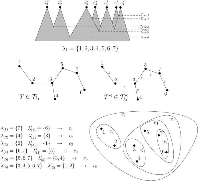
Figure 8: An example of pseudo-trajectory $\Psi^{\varepsilon}_{\lambda_{1}}$ ($\ell_{1}=7$) satisfying the constraint $\Delta\hskip-5.69046pt\Delta_{\lambda_{1},T^{\prec}}$, together with its minimally connected graph $T$, ordered graph $T^{\prec}$, and sequence of merged subforests $\left(\lambda_{(k)},\lambda^{\prime}_{(k)}\right)_{k}$. The roots of the trees $z_{i}^{*}=(x_{i}^{*},v_{i}^{*})$ and the clustering recollision times appear in the picture on the top.

More precisely, we define the map which associates to any ordered tree the sequence of merging clusters

$$\mathcal{T}^{\prec}_{\lambda_{1}}\ni T^{\prec}\mapsto\left(\lambda_{(k)},\lambda^{\prime}_{(k)}\right)_{k}$$

by the following iteration :

• start from $\lambda_{1}=\{1,\dots,\ell_{1}\}$;

• take the first edge $\{j_{1},j_{1}^{\prime}\}$ of $T^{\prec}$, and set $\left(\lambda_{(1)},\lambda^{\prime}_{(1)}\right)=\left(\{j_{1}\},\{j_{1}^{\prime}\}\right)$; these two elements are merged into a single cluster $c_{1}$; set $L_{1}:=c_{1}\cup\left(\lambda_{1}\setminus\{j_{1},j_{1}^{\prime}\}\right)$;

• at step $k>1$, take $\left(\lambda_{(k)},\lambda^{\prime}_{(k)}\right)$ of $L_{k-1}$ in such a way that $j_{k}\in\lambda_{(k)},j^{\prime}_{k}\in\lambda^{\prime}_{(k)}$ where $\{j_{k},j^{\prime}_{k}\}$ is the $k$-th edge of $T^{\prec}$, and merge them into a single cluster $c_{k}$; set $L_{k}:=c_{k}\cup\left(L_{k-1}\setminus\{\lambda_{(k)},\lambda^{\prime}_{(k)}\}\right)$. We can assume without loss of generality that $\max\lambda^{\prime}_{(k)}<\max\lambda_{(k)}$.

The last step is given by $\left(\lambda_{(\ell_{1}-1)},\lambda^{\prime}_{(\ell_{1}-1)}\right)$, which merges the two remaining clusters.

However this map is not a bijection, because the merged subforests do not specify which vertices of $j_{k}\in\lambda_{(k)}$ and $j^{\prime}_{k}\in\lambda^{\prime}_{(k)}$ are connected by the edge. A bijection is therefore given by

$$\mathcal{T}^{\prec}_{\lambda_{1}}\ni T^{\prec}\to\left(\lambda_{(k)},\lambda^{\prime}_{(k)},j_{k}\in\lambda_{(k)},j^{\prime}_{k}\in\lambda^{\prime}_{(k)}\right)_{k}\;.$$ (32.4)

We define the root of the subforest $\lambda_{(k)}$ by

$$x^{*}_{\lambda_{(k)}}:=x_{\max\lambda_{(k)}}^{*}\,,$$

and same definition for the root of $\lambda^{\prime}_{(k)}$. We can then define

$$\hat{x}_{k}:=x^{*}_{\lambda^{\prime}_{(k)}}-x^{*}_{\lambda_{(k)}}\,,\qquad k=1,\dots,\ell_{1}-1$$

as the relative position between the two recolliding subforests at time $t$. It is easy to see that, for any given root position $x^{*}_{\lambda_{1}}=x^{*}_{\ell_{1}}\in\mathbb{T}^{d}$, the map of translations

$$X^{*}_{\ell_{1}-1}=\left(x^{*}_{1},\dots,x^{*}_{\ell_{1}-1}\right)\mapsto\hat{X}_{\ell_{1}-1}:=\left(\hat{x}_{1},\dots,\hat{x}_{\ell_{1}-1}\right)$$ (32.5)

is one-to-one on $\mathbb{T}^{d(\ell_{1}-1)}$ and such that

$$dX^{*}_{\ell_{1}-1}=d\hat{X}_{\ell_{1}-1}\;.$$

Thus (32.5) is a legitimate change of variables in (31.1).

Our purpose is to prove iteratively that, for $k=\ell_{1}-1,\dots,1$, the variable $\hat{x}_{k}$ associated with the $k$-th clustering recollision has to be in a small set, the measure of which is uniformly small of size $O(1/\mu_{\varepsilon})$.

We define $\Psi^{\varepsilon}_{\lambda_{(k)}}$ (respectively $\Psi^{\varepsilon}_{\lambda^{\prime}_{(k)}}$) the pseudo-trajectory with starting particles $\lambda_{(k)}$ $(\lambda^{\prime}_{(k)})$. Since $\tau_{\rm{rec},k}\geq\left(\tau_{\rm{rec},s}\right)_{s>k}$, the collision trees in $\lambda_{1}\setminus\left(\lambda_{(k)}\cup\lambda^{\prime}_{(k)}\right)$ do not affect the subforests $\lambda_{(k)},\lambda^{\prime}_{(k)}$ in the time interval $(\tau_{\rm{rec},k},t)$. The clustering structure prescribed by $T^{\prec}$ implies that $\Psi^{\varepsilon}_{\lambda^{\prime}_{(k)}}$ and $\Psi^{\varepsilon}_{\lambda_{(k)}}$, regarded as independent trajectories, reach mutual distance ${\varepsilon}$ at some time $\tau_{\rm{rec},k}\in(0,\tau_{\rm{rec},k-1})$.

Given $\left(\hat{x}_{s}\right)_{s<k}$ fixed by the previous recollisions, we are going to vary $\hat{x}_{k}$ so that an external recollision between the subforests occurs. This corresponds to moving rigidly $\Psi^{\varepsilon}_{\lambda^{\prime}_{(k)}}$ and $\Psi^{\varepsilon}_{\lambda_{(k)}}$ by acting on their relative distance $\hat{x}_{k}$. In fact, the recollision condition depends only on this distance.

Given a sequence of merged subforests $\left(\lambda_{(k)},\lambda^{\prime}_{(k)}\right)_{k}$ and a set of variables $\left(\hat{x}_{s}\right)_{s<k}$ (with $|\hat{x}_{s}|>{\varepsilon}$), the $k-$th clustering recollision condition is defined by

$$\hat{x}_{k}\in\mathcal{B}_{k}:=\bigcup_{\tiny\begin{subarray}{c}\mbox{$q$ in the subforest $\lambda_{(k)}$}\\ \mbox{$q^{\prime}$ in the subforest $\lambda^{\prime}_{(k)}$}\end{subarray}}B_{qq^{\prime}}\,,$$

with

$$B_{qq^{\prime}}:=\Big{\{}\hat{x}_{k}\in\mathbb{T}^{d}\;\;:\;\;|x_{q^{\prime}}(\tau_{{\rm{rec}},k})-x_{q}(\tau_{{\rm{rec}},k})|={\varepsilon}\ \ \ \mbox{for some $\tau_{\rm{rec},k}\in(0,\tau_{{\rm{rec}},k-1})$}\Big{\}}\;.$$ (32.6)

Here $x_{q}(\tau),x_{q^{\prime}}(\tau)$ are the particle trajectories in the flows $\Psi^{\varepsilon}_{\lambda_{(k)}},\Psi^{\varepsilon}_{\lambda^{\prime}_{(k)}}$ (and $\tau$ is of course restricted to their existence times). In other words there exists a time $\tau_{\rm{rec},k}\in(0,\tau_{\rm{rec},k-1})$ and a vector $\omega_{\rm{rec},k}\in{\mathbb{S}}^{d-1}$ such that

$$x_{q^{\prime}}(\tau_{{\rm{rec}},k})-x_{q}(\tau_{{\rm{rec}},k})={\varepsilon}\,\omega_{{\rm{rec}},k}\,.$$ (32.7)

The particle trajectories $x_{q}(\tau),x_{q^{\prime}}(\tau)$ are piecewise affine (because there are almost surely a finite number of collisions and recollisions within the trees $\Psi^{\varepsilon}_{\lambda_{(k)}},\Psi^{\varepsilon}_{\lambda^{\prime}_{(k)}}$). We will denote by $v_{q}^{(\delta\tau_{j})},v_{q^{\prime}}^{(\delta\tau_{j})}$ the velocities of $q$ and $q^{\prime}$ on the interval $\delta\tau_{j}$. Moreover, $(x_{q}(\tau)-x_{q^{\prime}}(\tau))-(x^{*}_{\lambda_{(k)}}-x^{*}_{\lambda^{\prime}_{(k)}})$ does not depend on $\hat{x}_{k}:=x^{*}_{\lambda^{\prime}_{(k)}}-x^{*}_{\lambda_{(k)}}$, because all positions in the collision tree are translated rigidly. This means that $\hat{x}_{k}$ has to be in a tube of radius ${\varepsilon}$ around the parametric curve $(x^{*}_{\lambda_{(k)}}-x^{*}_{\lambda^{\prime}_{(k)}})-(x_{q}(\tau)-x_{q^{\prime}}(\tau))$. This tube is a union of cylinders, with two spherical caps at both ends (see Figure 9). Note however that we have to remove from this tube the ball corresponding to the exclusion at the creation time (or at time $t$ if $q$ and $q^{\prime}$ exist up to time $t$).

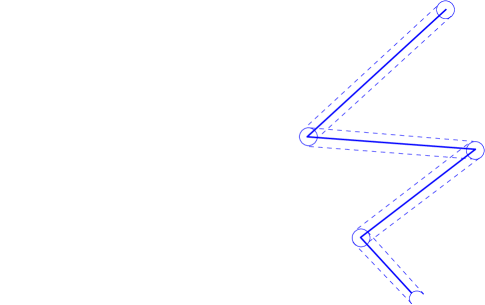
Figure 9: The tube $B_{qq^{\prime}}$ leading to a recollision between particles $q$ and $q^{\prime}$. The tube has section $\mu_{\varepsilon}^{-1}$.

Therefore

$$B_{qq^{\prime}}=\bigcup_{j}B_{qq^{\prime}}(\delta\tau_{j})$$

for a suitable finite decomposition of $(0,\tau_{\rm{rec},k-1})$ (depending on all the history). We therefore end up with the estimate (see Figure 9)

$$|B_{qq^{\prime}}|\leq\frac{C}{\mu_{\varepsilon}}\sum_{j}|v_{q}^{(\delta\tau_{j})}-v_{q^{\prime}}^{(\delta\tau_{j})}|\,|\delta\tau_{j}|$$

for some pure constant $C>0$ depending only on the dimension $d$.

We sum now over all $q,q^{\prime}$ to obtain an estimate of the set $\mathcal{B}_{k}$. To exploit the conservation of energy, we exchange the sums over $\delta\tau_{j}$ and over $q,q^{\prime}$. We get

$$|\mathcal{B}_{k}|\leq\frac{C}{\mu_{\varepsilon}}\sum_{j}|\delta\tau_{j}|\sum_{q,q^{\prime}}|v_{q}^{(\delta\tau_{j})}-v_{q^{\prime}}^{(\delta\tau_{j})}|\,.$$

Applying the Cauchy-Schwarz inequality, the sum over $q,q^{\prime}$ is bounded by

$$\sqrt{\sum_{q}\left(v_{q}^{(\delta\tau_{j})}\right)^{2}}\sqrt{K_{\lambda_{(k)}}}\,K_{\lambda^{\prime}_{(k)}}+\sqrt{\sum_{q^{\prime}}\left(v_{q^{\prime}}^{(\delta\tau_{j})}\right)^{2}}\sqrt{K_{\lambda^{\prime}_{(k)}}}\,K_{\lambda_{(k)}}\leq{\mathbb{V}}_{\lambda_{(k)}}\,\sqrt{K_{\lambda_{(k)}}}\,K_{\lambda^{\prime}_{(k)}}+{\mathbb{V}}_{\lambda^{\prime}_{(k)}}\,\sqrt{K_{\lambda^{\prime}_{(k)}}}\,K_{\lambda_{(k)}}$$

where we use the notations for energy and mass of subforests introduced at the beginning of this section. In the above inequality, we have used the independence of $\Psi^{\varepsilon}_{\lambda_{(k)}}$ and $\Psi^{\varepsilon}_{\lambda^{\prime}_{(k)}}$ on $[\tau_{{\rm{rec}},k},t]$, and bounded their energies in $\delta\tau_{j}$ with ${\mathbb{V}}_{\lambda_{(k)}}$ and ${\mathbb{V}}_{\lambda^{\prime}_{(k)}}$ respectively (see Eq.s (LABEL:eq:energia1)-(LABEL:eq:energia2)). Therefore we infer that

$$|\mathcal{B}_{k}| \leq\frac{C}{\beta_{0}^{1/2}\mu_{\varepsilon}}\int d\tau_{{\rm{rec}},k}{\bf 1}_{\tau_{{\rm{rec}},k}\leq\tau_{{\rm{rec}},k-1}}\,\left(\beta_{0}{\mathbb{V}}^{2}_{\lambda_{(k)}}+K_{\lambda_{(k)}}\right)\left(\beta_{0}{\mathbb{V}}^{2}_{\lambda^{\prime}_{(k)}}+K_{\lambda^{\prime}_{(k)}}\right)$$ (32.8)

$$=\frac{C}{\beta_{0}^{1/2}\mu_{\varepsilon}}\int d\tau_{{\rm{rec}},k}{\bf 1}_{\tau_{{\rm{rec}},k}\leq\tau_{{\rm{rec}},k-1}}\,\sum_{\begin{subarray}{c}j_{k}\in\lambda_{(k)}\\ j^{\prime}_{k}\in\lambda^{\prime}_{(k)}\end{subarray}}\Big{(}\beta_{0}{\mathbb{V}}^{2}_{j_{k}}+K_{j_{k}}\Big{)}\left(\beta_{0}{\mathbb{V}}^{2}_{j^{\prime}_{k}}+K_{j^{\prime}_{k}}\right)\;.$$

In this way we have obtained an estimate which depends only on the energy and the number of particles enclosed in the trees $\Psi^{\varepsilon}_{\lambda_{(k)}},\Psi^{\varepsilon}_{\lambda^{\prime}_{(k)}}$.

Coming back to Equation (31.1) we observe that, if $\Delta\hskip-5.69046pt\Delta_{\lambda_{1}}=1$, then there exist merged subforests such that $\hat{x}_{k}\in\mathcal{B}_{k}$ for $k=\ell_{1}-1,\dots,1$. Hence, iterating the procedure leading to (32.8) for $k=\ell_{1}-1,\dots,1$, leads to an upper bound on the cost of the clustering recollisions in $\lambda_{1}$:

$$\int\!\!dX^{*}_{\ell_{1}-1}\,\Delta\hskip-5.69046pt\Delta_{\lambda_{1}}\,{\bf 1}_{\mathcal{G}^{{\varepsilon}}}\big{(}\Psi^{\varepsilon}_{\lambda_{1}}\big{)}\leq\sum_{\left(\lambda_{(k)},\lambda^{\prime}_{(k)}\right)}\int\!\!d\hat{x}_{1}{\bf 1}_{\mathcal{B}_{1}}\!\int\!\!d\hat{x}_{2}\dots\!\int\!\!d\hat{x}_{\ell_{1}-1}{\bf 1}_{\mathcal{B}_{\ell_{1}-1}}$$ (32.9)

$$\qquad\leq\left(\frac{C}{\beta_{0}^{1/2}\mu_{\varepsilon}}\right)^{\ell_{1}-1}\int_{0}^{t}d\tau_{\rm{rec},1}\cdots\int_{0}^{\tau_{\rm{rec},\ell_{1}-2}}d\tau_{\rm{rec},\ell_{1}-1}\sum_{\left(\lambda_{(k)},\lambda^{\prime}_{(k)}\right)}\,\sum_{\begin{subarray}{c}j_{k}\in\lambda_{(k)}\\ j^{\prime}_{k}\in\lambda^{\prime}_{(k)}\end{subarray}}\,\prod_{k=1}^{\ell_{1}-1}\,\left(\beta_{0}{\mathbb{V}}^{2}_{j_{k}}+K_{j_{k}}\right)\left(\beta_{0}{\mathbb{V}}^{2}_{j^{\prime}_{k}}+K_{j^{\prime}_{k}}\right)$$

$$\qquad=\left(\frac{Ct}{\beta_{0}^{1/2}\mu_{\varepsilon}}\right)^{\ell_{1}-1}\frac{1}{(\ell_{1}-1)!}\sum_{\left(\lambda_{(k)},\lambda^{\prime}_{(k)}\right)}\,\sum_{\begin{subarray}{c}j_{k}\in\lambda_{(k)}\\ j^{\prime}_{k}\in\lambda^{\prime}_{(k)}\end{subarray}}\,\prod_{k=1}^{\ell_{1}-1}\,\left(\beta_{0}{\mathbb{V}}^{2}_{j_{k}}+K_{j_{k}}\right)\left(\beta_{0}{\mathbb{V}}^{2}_{j^{\prime}_{k}}+K_{j^{\prime}_{k}}\right)\;.$$

Using the bijection (32.4) and compensating the $1/(\ell_{1}-1)!$ with the ordering of the edges in $T^{\prec}$, we rewrite this result as

$$\int\!\!dX^{*}_{\ell_{1}-1}\Delta\hskip-5.69046pt\Delta_{\lambda_{1}}\,{\bf 1}_{\mathcal{G}^{{\varepsilon}}}\big{(}\Psi^{\varepsilon}_{\lambda_{1}}\big{)}\leq\left(\frac{Ct}{\beta_{0}^{1/2}\mu_{\varepsilon}}\right)^{\ell_{1}-1}\sum_{T\in\mathcal{T}_{\lambda_{1}}}\,\prod_{\{j,j^{\prime}\}\in E(T)}\,\left(\beta_{0}{\mathbb{V}}^{2}_{j}+K_{j}\right)\left(\beta_{0}{\mathbb{V}}^{2}_{j^{\prime}}+K_{j^{\prime}}\right)\;,$$

where $E(T)$ is the set of edges of $T$. Equivalently, we obtain (32.3).

– Clustering overlaps. We are now going to estimate the constraints associated with clustering overlaps in the pseudo-trajectory of the generic jungle ${\rho_{1}}$. Up to a renaming of the summation variables, we can assume that

$$\rho_{1}=\{\lambda_{1},\dots,\lambda_{r_{1}}\}\;.$$

The number of particles in the jungle at time $t$ is $|\rho_{1}|$, and at time 0 is $K_{\rho_{1}}=|\rho_{1}|+m_{\rho_{1}}$. We recall that each forest $\lambda_{i}$ has a root $x^{*}_{\lambda_{i}}$, which did not play any role in the previous estimate of clustering recollisions. We call $x^{*}_{\rho_{1}}:=x^{*}_{\lambda_{r_{1}}}$ the root of the jungle.

Proposition 32.2.

Consider some forests $\lambda_{1},\dots,\lambda_{r_{1}}$ whose internal dynamics is fixed (prescribed by the velocities and relative positions at time $t$, as well as the creation parameters). The set of configurations $Z_{|\rho_{1}|}^{*}$ at time $t$ compatible with the jungle $\rho_{1}=\{\lambda_{1},\dots,\lambda_{r_{1}}\}$ on $[0,t]$ satisfies the following estimate :

$$\int\!\!dx^{*}_{\lambda_{1}}\cdots dx^{*}_{\lambda_{r_{1}-1}}|\varphi_{\rho_{1}}|\leq\left(\frac{C}{\beta_{0}^{1/2}\mu_{\varepsilon}}\right)^{r_{1}-1}\,\left(t+{\varepsilon}\right)^{r_{1}-1}\sum_{T\in\mathcal{T}_{\rho_{1}}}\,\prod_{\lambda_{j}\in\rho_{1}}\,\left(\beta_{0}{\mathbb{V}}^{2}_{\lambda_{j}}+K_{\lambda_{j}}\right)^{d_{\lambda_{j}}(T)}\;.$$ (32.10)

The argument is similar, but not identical, to the one just seen for clustering recollisions. Below we shall indicate the differences, without repeating the identical parts.

By definition of $\varphi_{\rho_{1}}$, and by Definition 18.1, the clustering overlaps are extracted from the graph of all overlaps between the forests $\{\lambda_{1},\dots,\lambda_{r_{1}}\}$ via the Penrose algorithm : we denote by $(\lambda_{j_{1}},\lambda_{j^{\prime}_{1}}),\cdots,(\lambda_{j_{r_{1}-1}},\lambda_{j^{\prime}_{r_{1}-1}})$ the (ordered) edges of the resulting minimally connected graph $T\in\mathcal{T}_{\rho_{1}}$. Then, thanks to the tree inequality stated in Proposition 9.3,

$$|\varphi_{\rho_{1}}|\leq\sum_{T\in\mathcal{T}_{\rho_{1}}}\,\prod_{\{\lambda_{j},\lambda_{j^{\prime}}\}\in E(T)}\,{\bf 1}_{\lambda_{j}\sim_{o}\lambda_{j^{\prime}}}\,.$$ (32.11)

Note that, as mentioned in Section 18, we have more flexibility when dealing with overlaps than with recollisions, as $\left(\Psi^{\varepsilon}_{\lambda_{j}}\right)_{1\leq j\leq r_{1}}$ are completely independent trajectories, whatever the ordering of the overlap times. We therefore have more freedom in choosing the integration variables.

We can then define

$$\hat{x}_{k}:=x^{*}_{\lambda^{\prime}_{[k]}}-x^{*}_{\lambda_{[k]}}\,,\qquad k=1,\dots,r_{1}-1$$

as the relative position between the two overlapping forests at time $t$. As in the case of clustering recollisions, for any given root position $x^{*}_{\rho_{1}}:=x^{*}_{\lambda_{r_{1}}}\in\mathbb{T}^{d}$, the map of translations

$$\left(x^{*}_{\lambda_{1}},\dots,x^{*}_{\lambda_{r_{1}-1}}\right)\longmapsto\hat{X}_{r_{1}-1}:=\left(\hat{x}_{1},\dots,\hat{x}_{r_{1}-1}\right)$$ (32.12)

is one-to-one on $\mathbb{T}^{d(r_{1}-1)}$ and it has unit Jacobian determinant. Thus (32.12) is a legitimate change of variables in (31.1).

Given a graph $T\in\mathcal{T}_{\rho_{1}}$ and the corresponding sequence $\left(\lambda_{[k]},\lambda^{\prime}_{[k]}\right)_{k}$, the $k-$th clustering overlap condition is defined by

$$\hat{x}_{k}\in\tilde{\mathcal{B}}_{k}:=\bigcup_{\tiny\begin{subarray}{c}\mbox{$q$ in the forest $\lambda_{[k]}$}\\ \mbox{$q^{\prime}$ in the forest $\lambda^{\prime}_{[k]}$}\end{subarray}}\tilde{B}_{qq^{\prime}}\,,$$

with

$$\tilde{B}_{qq^{\prime}}=\Big{\{}\hat{x}_{k}\in\mathbb{T}^{d}\ :\ \exists\tau\in[0,t]\quad\text{such that}\quad|x_{q}(\tau)-x_{q^{\prime}}(\tau)|\leq{\varepsilon}\Big{\}}$$

where we used (18.3), and $x_{q}(\tau),x_{q^{\prime}}(\tau)$ are the particle trajectories in the flows $\Psi^{\varepsilon}_{\lambda_{[k]}},\Psi^{\varepsilon}_{\lambda^{\prime}_{[k]}}$. This set has small measure

$$|\tilde{\mathcal{B}}_{k}|\leq\frac{C}{\beta_{0}^{1/2}\mu_{\varepsilon}}\left(t+{\varepsilon}\right)\left(\beta_{0}{\mathbb{V}}^{2}_{\lambda_{[k]}}+K_{\lambda_{[k]}}\right)\left(\beta_{0}{\mathbb{V}}^{2}_{\lambda^{\prime}_{[k]}}+K_{\lambda^{\prime}_{[k]}}\right)$$ (32.13)

for some constant $C>0$. Notice that the correction of $O({\varepsilon})$ comes from the extremal spherical caps of the tubes in Figure 9 (since ${\bf 1}_{\lambda_{[k]}\sim_{o}\lambda^{\prime}_{[k]}}=1$ inside those regions).

Remark 32.3.

Note that overlaps can be classified in two types

• those arising at time $t$ or involving a particle $q$ at its creation time $t_{q}$ : in this case, the distance between the overlapping particles at $\tau_{\rm{ov}}$ satisfies only the inequality

  $$|x_{q}(\tau_{\rm{ov}})-x_{q^{\prime}}(\tau_{\rm{ov}})|\leq{\varepsilon}\,.$$

  This corresponds to one spherical end of the tube in Figure 9;

• and the regular ones, for which the two overlapping particles are exactly at distance ${\varepsilon}$ at $\tau_{\rm{ov}}$. We then have the same parametrization as for recollisions

  $$x_{q}(\tau_{\rm{ov}})-x_{q^{\prime}}(\tau_{\rm{ov}})={\varepsilon}\omega_{\rm{ov}}\,.$$ (32.14)

  This corresponds to the tube in Figure 9 minus the spherical end.

We finally obtain (32.10).

– Initial clustering. Finally, we are going to estimate the non-overlap constraints in the initial data, which are encoded in (17.1).

Recall that $f^{{\varepsilon}0}_{\{1,\dots,r\}}(\Psi^{{\varepsilon}0}_{\rho_{1}},\dots,\Psi^{{\varepsilon}0}_{\rho_{r}})$ is a measure of the correlations between all the different clusters of particles $\Psi^{{\varepsilon}0}_{\rho_{1}},\dots,\Psi^{{\varepsilon}0}_{\rho_{r}}$ at time zero, and its definition has been adapted to reconstruct the dynamical cumulants. An estimate of this correlation is obtained by integrating over the root coordinates of the jungles $x^{*}_{\rho_{1}},\dots,x^{*}_{\rho_{r-1}}$, as stated in the following proposition.

We recall that $K_{\rho_{i}}:=m_{\rho_{i}}+|\rho_{i}|$ denotes the number of particles in the configuration $\Psi^{{\varepsilon},0}_{\rho_{i}}$ at time 0, and that $\displaystyle K:=\sum_{i=1}^{r}K_{\rho_{i}}=m+n$.

Proposition 32.4.

Under Assumption (1.5), there exists $C>0$ (depending only on the dimension $d$) such that, for ${\varepsilon}$ small enough,

$$\int_{\mathbb{T}^{d(r-1)}}|f^{{\varepsilon}0}_{\{1,\dots,r\}}(\Psi^{{\varepsilon}0}_{\rho_{1}},\dots,\Psi^{{\varepsilon}0}_{\rho_{r}})|\,dx^{*}_{\rho_{1}}\dots dx^{*}_{\rho_{r-1}}\leq(r-2)!\,(CC_{0})^{K}\,\exp\Big{(}-\frac{{\beta}_{0}}{2}{\mathbb{V}}^{2}\Big{)}\,{\varepsilon}^{d({r-1)}}$$

for all $\Psi^{{\varepsilon}0}_{\rho_{i}}\in{\mathcal{D}}^{{\varepsilon}}_{K_{\rho_{i}}}$ at time 0. We have used the convention $0!=(-1)!=1$.

Recall that $f^{{\varepsilon}0}_{\{1,\dots,r\}}$ is extended to $\mathbb{D}^{K}\setminus{\mathcal{D}}^{{\varepsilon}}_{K}$ by setting $F^{{\varepsilon}0}_{\omega_{i}}=0$ in (17.1) wherever it is not defined.

The following proof is an application of known cluster expansion techniques, see e.g. [PU09] and references therein.

Démonstration.

Set $Z_{K}:=(\Psi^{{\varepsilon}0}_{\rho_{1}},\dots,\Psi^{{\varepsilon}0}_{\rho_{r}})$ with $\Psi^{{\varepsilon}0}_{\rho_{i}}\in{\mathcal{D}}^{{\varepsilon}}_{K_{\rho_{i}}}$ at time 0. To make notation lighter we shall omit the superscripts ^ε0 and also omit to specify the exclusion constraints inside each $\Psi^{\varepsilon}_{\rho_{i}}$ in the sequel. We define $\Phi_{r+p}$ the indicator function of the mutual exclusion between the elements of the set $\{\Psi^{\varepsilon}_{\rho_{1}},\dots,\Psi^{\varepsilon}_{\rho_{r}},\bar{z}_{1},\dots,\bar{z}_{p}\}$ (where $\Psi^{\varepsilon}_{\rho_{1}},\dots,\Psi^{\varepsilon}_{\rho_{r}}$ form $r$ clusters and $\bar{z}_{1},\dots,\bar{z}_{p}$ are the configurations of $p$ single particles):

$$\Phi_{r+p}=\prod_{h\neq h^{\prime}}{\bf 1}_{\eta_{h}\not\sim\eta_{h^{\prime}}}\,,$$

with $(\eta_{1},\dots,\eta_{r+p})=(\Psi^{\varepsilon}_{\rho_{1}},\dots,\Psi^{\varepsilon}_{\rho_{r}},\bar{z}_{1},\dots,\bar{z}_{p})$ and $``\eta_{h}\not\sim\eta_{h^{\prime}}"$ meaning that the minimum distance between elements of $\eta_{h}$ and $\eta_{h^{\prime}}$ is larger than ${\varepsilon}$. So we start from

$$F^{{\varepsilon}0}_{K}(Z_{K})=\frac{(f^{0})^{\otimes K}(Z_{K})}{\mathcal{Z}^{\varepsilon}}\sum_{p\geq 0}\frac{\mu_{\varepsilon}^{p}}{p!}\int_{\mathbb{D}^{p}}(f^{0})^{\otimes p}(\bar{Z}_{p})\,\Phi_{r+p}(\Psi^{\varepsilon}_{\rho_{1}},\dots,\Psi^{\varepsilon}_{\rho_{r}},\bar{Z}_{p})\,d\bar{Z}_{p}\,.$$ (32.15)

We want to expand $\Phi_{r+p}$ in order to compensate the factor $\mathcal{Z}^{\varepsilon}$ whose definition we recall

$$\mathcal{Z}^{\varepsilon}:=\sum_{p\geq 0}\frac{\mu_{\varepsilon}^{p}}{p!}\int_{\mathbb{D}^{p}}(f^{0})^{\otimes p}(\bar{Z}_{p})\,\Phi_{p}(\bar{Z}_{p})\,d\bar{Z}_{p}\,,$$ (32.16)

and to identify the elements in the decomposition

$$F^{{\varepsilon}0}_{K}(\Psi^{\varepsilon}_{\rho_{1}},\dots,\Psi^{\varepsilon}_{\rho_{r}})=\sum_{s=1}^{r}\sum_{\sigma\in\mathcal{P}^{s}_{r}}\prod_{i=1}^{s}f^{{\varepsilon}0}_{|\sigma_{i}|}(\Psi^{\varepsilon}_{\sigma_{i}})\,.$$

This will enable us to compute, and estimate, $f^{{\varepsilon}0}_{\{1,\dots,r\}}(\Psi^{\varepsilon}_{\rho_{1}},\dots,\Psi^{\varepsilon}_{\rho_{r}})$. To do so, we naturally develop $\Phi_{r+p}$ into $s$ clusters (each of them corresponding to one connected graph containing at least one element of $\{\Psi^{\varepsilon}_{\rho_{1}},\dots,\Psi^{\varepsilon}_{\rho_{r}}\}$), plus a background $\bar{\sigma}_{0}$ of mutually excluding particles (for which we do not expand the exclusion condition). Such a partition can be reconstructed isolating first the background component, and then splitting $\{\Psi^{\varepsilon}_{\rho_{1}},\dots,\Psi^{\varepsilon}_{\rho_{r}}\}$ in $s$ parts, to which we adjoin the remaining single particles (see Figure 10).

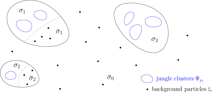
Figure 10: Initial configurations are decomposed in $s$ clusters containing at least one jungle $\Psi^{\varepsilon}_{\rho_{1}},\dots,\Psi^{\varepsilon}_{\rho_{r}}$, plus a background of mutually excluding particles (for which we do not expand the exclusion condition).

This amounts to introducing truncated functions $\varphi$ via the following formula:

$$\Phi_{r+p}(\Psi^{\varepsilon}_{\rho_{1}},\dots,\Psi^{\varepsilon}_{\rho_{r}},\bar{Z}_{p})\!=\!\!\sum_{\bar{\sigma}_{0}\subset\{1,\dots,p\}}\Phi_{|\bar{\sigma}_{0}|}(\bar{Z}_{\bar{\sigma}_{0}})\sum_{s=1}^{r}\sum_{\sigma\in\mathcal{P}^{s}_{r}}\,\sum_{\begin{subarray}{c}\bar{\sigma}_{1},\dots,\bar{\sigma}_{s}\subset\{1,\cdots,p\}\\ \cup_{i=0}^{s}\bar{\sigma}_{i}=\{1,\dots,p\}\\ \bar{\sigma}_{k}\cap\bar{\sigma}_{h}=\emptyset,k\neq h\end{subarray}}\,\prod_{i=1}^{s}\varphi(\Psi^{\varepsilon}_{\sigma_{i}},\bar{Z}_{\bar{\sigma}_{i}})\;.$$ (32.17)

Note that the $\bar{\sigma}_{i}$ may be empty (in particular all $\bar{\sigma}_{i}$ are empty if $|\bar{\sigma}_{0}|=p$). By (9.1), we see that

$$\varphi(\Psi^{\varepsilon}_{\rho_{1}},\dots,\Psi^{\varepsilon}_{\rho_{r}},\bar{Z}_{p})=\sum_{G\in\mathcal{C}_{r+p}}\prod_{(h,h^{\prime})\in E(G)}(-{\bf 1}_{\eta_{h}\sim\eta_{h^{\prime}}})\,,$$

where the sum runs over the set of connected graphs with $r+p$ vertices; more generally,

$$\varphi(\Psi^{\varepsilon}_{\sigma_{i}},\bar{Z}_{\bar{\sigma}_{i}})=\sum_{G\in\mathcal{C}_{|\sigma_{i}|+|\bar{\sigma}_{i}|}}\prod_{(h,h^{\prime})\in E(G)}(-{\bf 1}_{\eta_{h}\sim\eta_{h^{\prime}}})\,.$$

Using the symmetry in the exchange of particle labels, we get, denoting $\bar{s}_{i}:=|\bar{\sigma}_{i}|$,

$$\binom{p}{\bar{s}_{1}}\binom{p-\bar{s}_{1}}{\bar{s}_{2}}\dots\binom{p-\bar{s}_{1}-\dots-\bar{s}_{s-1}}{\bar{s}_{s}}={p!\over\bar{s}_{0}!\;\bar{s}_{1}!\dots\bar{s}_{s}!}$$

choices for the repartition of the background particles, so that

$$\sum_{p\geq 0}\frac{1}{p!}\int_{\mathbb{D}^{p}}\,\Phi_{r+p}(\Psi^{\varepsilon}_{\rho_{1}},\dots,\Psi^{\varepsilon}_{\rho_{r}},\bar{Z}_{p})\,d\bar{Z}_{p}=\sum_{s=1}^{r}\sum_{\sigma\in\mathcal{P}^{s}_{r}}\sum_{p\geq 0}\sum_{\begin{subarray}{c}\bar{s}_{0},\dots,\bar{s}_{s}\geq 0\\ \sum\bar{s}_{i}=p\end{subarray}}\int_{\mathbb{D}^{p}}\frac{\Phi_{\bar{s}_{0}}(\bar{Z}_{\bar{s}_{0}})}{\bar{s}_{0}!}\prod_{i=1}^{s}\frac{\varphi(\Psi^{\varepsilon}_{\sigma_{i}},\bar{Z}_{\bar{s}_{i}})}{\bar{s}_{i}!}d\bar{Z}_{p}\;.$$

Therefore, plugging (32.17) into (32.15) first and then using (32.16), we obtain

$$F^{{\varepsilon}0}_{K}(Z_{K}) =\frac{(f^{0})^{\otimes K}(Z_{K})}{\mathcal{Z}^{\varepsilon}}\sum_{s=1}^{r}\sum_{\sigma\in\mathcal{P}^{s}_{r}}\sum_{p\geq 0}\sum_{\begin{subarray}{c}\bar{s}_{0},\dots,\bar{s}_{s}\geq 0\\ \sum\bar{s}_{i}=p\end{subarray}}\left(\frac{\mu_{\varepsilon}^{\bar{s}_{0}}}{\bar{s}_{0}!}\int(f^{0})^{\otimes\bar{s}_{0}}(\bar{Z}_{\bar{s}_{0}})\Phi_{\bar{s}_{0}}(\bar{Z}_{\bar{s}_{0}})d\bar{Z}_{\bar{s}_{0}}\right)$$

$$\ \ \ \ \ \ \ \ \ \ \ \ \ \ \ \ \ \ \ \ \ \ \ \ \ \ \ \times\prod_{i=1}^{s}\frac{\mu_{\varepsilon}^{\bar{s}_{i}}}{\bar{s}_{i}!}\int(f^{0})^{\otimes\bar{s}_{i}}(\bar{Z}_{\bar{s}_{i}})\varphi(\Psi^{\varepsilon}_{\sigma_{i}},\bar{Z}_{\bar{s}_{i}})d\bar{Z}_{\bar{s}_{i}}$$

$$=(f^{0})^{\otimes K}(Z_{K})\sum_{s=1}^{r}\sum_{\sigma\in\mathcal{P}^{s}_{r}}\prod_{i=1}^{s}\sum_{\bar{s}_{i}\geq 0}\frac{\mu_{\varepsilon}^{\bar{s}_{i}}}{\bar{s}_{i}!}\int(f^{0})^{\otimes\bar{s}_{i}}(\bar{Z}_{\bar{s}_{i}})\varphi(\Psi^{\varepsilon}_{\sigma_{i}},\bar{Z}_{\bar{s}_{i}})d\bar{Z}_{\bar{s}_{i}}\,,$$

hence finally

$$f^{{\varepsilon}0}_{\{1,\dots,r\}}(\Psi^{\varepsilon}_{\rho_{1}},\dots,\Psi^{\varepsilon}_{\rho_{r}})=(f^{0})^{\otimes K}(Z_{K})\sum_{p\geq 0}\frac{\mu_{\varepsilon}^{p}}{p!}\int(f^{0})^{\otimes p}(\bar{Z}_{p})\varphi(\Psi^{\varepsilon}_{\rho_{1}},\dots,\Psi^{\varepsilon}_{\rho_{r}},\bar{Z}_{p})d\bar{Z}_{p}\,.$$ (32.18)

Applying again Proposition 9.3 implies that $\varphi$ is bounded by

$$|\varphi(\Psi^{\varepsilon}_{\rho_{1}},\dots,\Psi^{\varepsilon}_{\rho_{r}},\bar{Z}_{p})|\leq\sum_{T\in\mathcal{T}_{r+p}}\prod_{(h,h^{\prime})\in E(T)}{\bf 1}_{\eta_{h}\sim\eta_{h^{\prime}}}$$ (32.19)

where $\mathcal{T}_{r+p}$ is the set of minimally connected graphs with $r+p$ vertices labelled by $\Psi^{\varepsilon}_{\rho_{1}},\dots,\Psi^{\varepsilon}_{\rho_{r}},\bar{z}_{1},\dots,\bar{z}_{p}$.

By Lemma 10.1, the number of minimally connected graphs with specified vertex degrees $d_{1},\dots,d_{r+p}$ is given by

$${(r+p-2)!}/{\displaystyle\prod_{i=1}^{r+p}(d_{i}-1)!}\,.$$

On the other hand, the product of indicator functions in (32.19) is a sequence of $r+p-1$ constraints, confining the space coordinates to balls of size ${\varepsilon}$ centered at the positions of the clusters $\Psi^{\varepsilon}_{\rho_{1}},\dots,\Psi^{\varepsilon}_{\rho_{r}},\bar{z}_{1},\dots,\bar{z}_{p}$. Such clusters have cardinality $K_{\rho_{1}},\dots,K_{\rho_{r}}\geq 1$ with the constraint

$$\sum_{i}K_{\rho_{i}}=K\;.$$

We deduce that for some $C>0$ depending only on the dimension $d$

$$\int_{\mathbb{T}^{d(r-1)}}|f^{{\varepsilon}0}_{\{1,\dots,r\}}(\Psi^{\varepsilon}_{\rho_{1}},\dots,\Psi^{\varepsilon}_{\rho_{r}})|dx^{*}_{\rho_{1}}\dots dx^{*}_{\rho_{r-1}}$$

$$\qquad\leq(CC_{0})^{K}{\varepsilon}^{d(r-1)}e^{-\frac{{\beta}_{0}}{2}{\mathbb{V}}^{2}}\sum_{p\geq 0}\frac{(r+p-2)!}{p!}(CC_{0}{\varepsilon}^{d}\mu_{\varepsilon})^{p}\sum_{d_{1},\dots,d_{r+p}\geq 1}\frac{\prod_{i=1}^{r}K_{\rho_{i}}^{d_{i}}}{\prod_{i=1}^{r+p}(d_{i}-1)!}$$

$$\qquad\leq(CC_{0})^{K}{\varepsilon}^{d(r-1)}e^{-\frac{{\beta}_{0}}{2}{\mathbb{V}}^{2}}\sum_{p\geq 0}\frac{(r+p-2)!}{p!}(C_{0}{\varepsilon}^{d}\mu_{\varepsilon})^{p}\,e^{2K+p}$$

$$\qquad\leq(CC_{0})^{K}{\varepsilon}^{d(r-1)}e^{-\frac{{\beta}_{0}}{2}{\mathbb{V}}^{2}}2^{r-2}(r-2)!\sum_{p\geq 0}(CC_{0}{\varepsilon}^{d}\mu_{\varepsilon})^{p}\,e^{2K+p}\;.$$

In the second inequality we used that

$$\prod_{i=1}^{r}\sum_{d_{i}\geq 1}\frac{K_{\rho_{i}}^{d_{i}}}{(d_{i}-1)!}\leq\prod_{i=1}^{r}K_{\rho_{i}}e^{K_{\rho_{i}}}\leq\prod_{i=1}^{r}e^{2K_{\rho_{i}}}=e^{2K}\;.$$

Since $C{\varepsilon}^{d}\mu_{\varepsilon}$ is arbitrarily small with ${\varepsilon}$, this proves Proposition 32.4. ∎

33 Decay estimate for the cumulants

We shall now prove the bound provided in Theorem 10. In the previous section, we considered a nested partition $\lambda\hookrightarrow\rho\hookrightarrow\sigma$ (with $|\sigma|=1$) of the set $\{1^{*},\dots,n^{*}\}$. We fixed the velocities $V_{n}^{*}$ as well as the collision parameters of the pseudo-trajectories $(m,a,T_{m},V_{m},\Omega_{m})$. We then exhibited $n-1$ “independent” conditions on the positions $X_{n}^{*}$ for the pseudo-trajectories to be compatible with the partitions $\lambda,\rho$. Now we shall conclude the proof of Theorem 10, by integrating successively on all the available parameters. The order of integration is pictured in Figure 11.

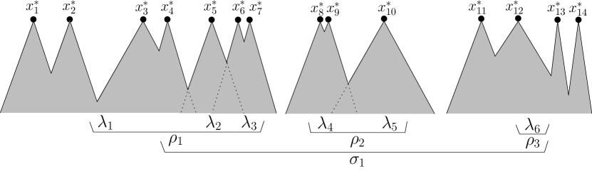
Figure 11: In this contribution to the cumulant of order $n=14$, we integrate over the positions of the roots in the following order: (i) first we integrate over the initial clustering $\hat{x}_{\rho_{2}}=x^{*}_{10}-x^{*}_{14}$ and $\hat{x}_{\rho_{1}}=x^{*}_{7}-x^{*}_{14}$; (ii) secondly over the clustering overlaps $\hat{x}_{\lambda_{4}}=x^{*}_{9}-x^{*}_{10}$ and $\hat{x}_{\lambda_{1}}=x^{*}_{4}-x^{*}_{5}\,,\hat{x}_{\lambda_{2}}=x^{*}_{5}-x^{*}_{7}$; (iii) finally over the clustering recollisions : $\hat{x}^{(\lambda_{1})}_{3}=x_{2}^{*}-x_{3}^{*},\quad\hat{x}^{(\lambda_{1})}_{2}=x_{1}^{*}-x_{2}^{*},\quad\hat{x}^{(\lambda_{1})}_{1}=x_{3}^{*}-x_{4}^{*},\quad\hat{x}^{(\lambda_{3})}_{1}=x_{6}^{*}-x_{7}^{*},\quad\hat{x}^{(\lambda_{4})}_{1}=x_{8}^{*}-x_{9}^{*},\quad\hat{x}^{(\lambda_{6})}_{3}=x^{*}_{13}-x^{*}_{14},\quad\hat{x}^{(\lambda_{6})}_{2}=x_{12}^{*}-x_{13}^{*},\quad\hat{x}^{(\lambda_{6})}_{1}=x_{11}^{*}-x_{12}^{*}$. Notice that the variable $x^{*}_{14}$ remains free.

For the proof of the first two statements in Theorem 10, we start by controlling the weight, simply using the bounds

$$|\mathcal{H}(\Psi^{\varepsilon}_{n})|\leq\prod_{i=1}^{n}\|H^{(i)}\|_{\infty}\quad\hbox{ or }\quad|\mathcal{H}(\Psi^{\varepsilon}_{n})|\leq e^{{\alpha n}+\frac{\beta_{0}}{4}{\mathbb{V}}^{2}}\,.$$ (33.1)

Then we use that nothing depends on the root coordinates of the jungles $x^{*}_{\rho_{1}},\dots,x^{*}_{\rho_{r-1}}$ inside the integrand in (31.1), except the initial datum $f^{{\varepsilon}0}_{\{1,\dots,r\}}$. Therefore by Fubini and according to Proposition 32.4,

$$\int_{\mathbb{T}^{d(r-1)}}|f^{{\varepsilon}0}_{\{1,\dots,r\}}(\Psi^{{\varepsilon}0}_{\rho_{1}},\dots,\Psi^{{\varepsilon}0}_{\rho_{r}})|dx^{*}_{\rho_{1}}\dots dx^{*}_{\rho_{r-1}}\leq(r-2)!\,(CC_{0})^{K}\,\exp\Big{(}-\frac{{\beta}_{0}}{2}{\mathbb{V}}^{2}\Big{)}\,{\varepsilon}^{d({r-1)}}$$ (33.2)

for some $C>0$, uniformly with respect to all other parameters.

Next, the clustering condition on the jungles gives an extra smallness when integrating over the roots of the forests (see (32.10))

$$\prod_{i=1}^{r}\int|\varphi_{\rho_{i}}|\;\prod_{j=1}^{r_{i}-1}dx^{*}_{\lambda_{j}}\leq\left(\frac{C}{\beta_{0}^{1/2}\mu_{\varepsilon}}\right)^{\ell-r}\,\left(t+{\varepsilon}\right)^{\ell-r}\,\prod_{i=1}^{r}\,\sum_{T\in\mathcal{T}_{\rho_{i}}}\,\,\prod_{\lambda_{j}\in\rho_{i}}\,\left(\beta_{0}{\mathbb{V}}^{2}_{\lambda_{j}}+K_{\lambda_{j}}\right)^{d_{\lambda_{j}}(T)}\;,$$ (33.3)

uniformly with respect to all other parameters, for some possibly larger constant $C$.

The clustering condition on the forests gives finally an extra smallness when integrating over the remaining variables $\hat{x}_{k}$, according to (32.3). Notice however that the latter inequality cannot be directly applied to (18.1), due to the presence of the cross section factors (31.5) in the measure (14.5).

It is then useful to combine the estimate with the sum over trees $a_{|\lambda_{i}}$. The argument is depicted in Figure 12. We will present the arguments for $\lambda_{1}$, assuming without loss of generality that $\lambda_{1}=\{1,\dots,\ell_{1}\}$. We will denote by $\tilde{a}$ the restriction of the tree $a$ to $\lambda_{1}$ with fixed total numbers of particles $K_{1},\cdots,K_{\ell_{1}}$, and by $\tilde{a}_{k}$, $\mathcal{C}_{k}$ the tree variables and the cross section factors associated with the $s_{k}$ creations occurring in the time interval $(\tau_{\rm{rec},k},\tau_{\rm{rec},k-1})$ for $1\leq k\leq\ell_{1}$.

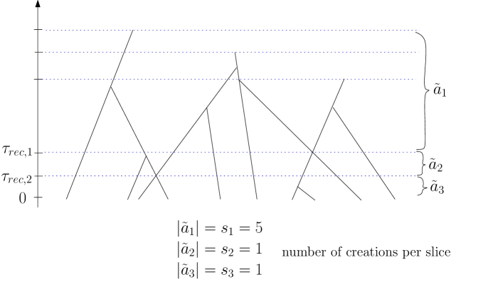
Figure 12: Integration over time slices.

As in the first line of (LABEL:eq:_external_recollision_cost_trees_0), we have that

$$\sum_{\tilde{a}}\int\!\!dX^{*}_{\ell_{1}-1}\,\Delta\hskip-5.69046pt\Delta_{\lambda_{1}}\,{\bf 1}_{\mathcal{G}^{{\varepsilon}}}\big{(}\Psi^{\varepsilon}_{\lambda_{1}}\big{)}|\mathcal{C}\big{(}\Psi^{\varepsilon}_{\lambda_{1}}\big{)}|$$ (33.4)

$$\qquad\leq\sum_{\left(\lambda_{(k)},\lambda^{\prime}_{(k)}\right)}\sum_{\tilde{a}_{1}}|\mathcal{C}^{\varepsilon}_{1}\,\big{(}\Psi_{\lambda_{1}}\big{)}|\int\!\!d\hat{x}_{1}{\bf 1}_{\mathcal{B}_{1}}\!\sum_{\tilde{a}_{2}}|\mathcal{C}_{2}\big{(}\Psi^{\varepsilon}_{\lambda_{1}}\big{)}|\int\!\!d\hat{x}_{2}\dots\!\int\!\!d\hat{x}_{\ell_{1}-1}{\bf 1}_{\mathcal{B}_{\ell_{1}-1}}\,\sum_{\tilde{a}_{\ell_{1}}}|\mathcal{C}_{\ell_{1}}\big{(}\Psi^{\varepsilon}_{\lambda_{1}}\big{)}|\,.$$

We can therefore apply iteratively the inequality (32.8) and the classical Cauchy-Schwarz argument used in Lanford’s proof. Denote by

$$S_{k}:=\sum_{i=1}^{k}s_{i}$$

the number of particles added before time $\tau_{\rm{rec},k}$, so that

$$S_{\ell_{1}}=m_{\lambda_{1}}$$

(denoting abusively $\tau_{\rm{rec},\ell_{1}}=0$). We get

$$\sum_{\tilde{a}_{k}}\big{|}\mathcal{C}_{k}\big{(}\Psi_{\lambda_{1}}\big{)}\big{|} \leq\prod_{s=S_{k-1}+1}^{S_{k}}\left(\sum_{u=1}^{s-1}|v_{s}-v_{u}(t_{s})|+\sum_{u=1}^{\ell_{1}}|v_{s}-v_{u}^{*}(t_{s})|\right)$$ (33.5)

$$\leq\prod_{s=S_{k-1}+1}^{S_{k}}\left((\ell_{1}+s-1)|v_{s}|+\sum_{u=1}^{s-1}|v_{u}(t_{s})|+\sum_{u=1}^{\ell_{1}}|v_{u}^{*}(t_{s})|\right)$$

$$\leq{1\over\beta_{0}^{s_{k}/2}}\prod_{s=S_{k-1}+1}^{S_{k}}\left((\ell_{1}+m_{\lambda_{1}})(1+\beta_{0}^{1/2}|v_{s}|)+\beta_{0}|{\mathbb{V}}_{\lambda_{1}}|^{2}\right)$$

and

$$\sum_{\tilde{a}}\int\!\!dX^{*}_{\ell_{1}-1}\,\Delta\hskip-5.69046pt\Delta_{\lambda_{1}}\,{\bf 1}_{\mathcal{G}^{{\varepsilon}}} \big{(}\Psi_{\lambda_{1}}\big{)}|\mathcal{C}\big{(}\Psi_{\lambda_{1}}\big{)}|\leq\left(\frac{C}{\beta_{0}^{1/2}\mu_{\varepsilon}}\right)^{\ell_{1}-1}{\color[rgb]{0,0,0}\left(\frac{1}{\beta_{0}}\right)^{m_{\lambda_{1}}/2}}\,\left(t+{\varepsilon}\right)^{\ell_{1}-1}\,$$ (33.6)

$$\times\sum_{T\in\mathcal{T}_{\lambda_{1}}}\,\prod_{j\in\lambda_{1}}\,\left(\beta_{0}{\mathbb{V}}^{2}_{j}+K_{j}\right)^{d_{j}(T)}\prod_{s=1}^{m_{\lambda_{1}}}\left((\ell_{1}+m_{\lambda_{1}})(1+\beta_{0}^{1/2}|v_{s}|)+\beta_{0}|{\mathbb{V}}_{\lambda_{1}}|^{2}\right),$$

for some positive $C$.

Recall that

$$\exp\left(-\frac{\beta_{0}}{16m}|V|^{2}\right)\beta_{0}|V|^{2}\leq Cm.$$

Combining (33.6) with the bound (33.1) on $\mathcal{H}$, (33.2) and (33.3) leads therefore to

$$\int\,\Big{|}\,\sum_{a}\,\prod_{i=1}^{\ell}\,\Delta\hskip-5.69046pt\Delta_{\lambda_{i}}\;\mathcal{C}\big{(}\Psi^{\varepsilon}_{\lambda_{i}}\big{)}\;{\bf 1}_{\mathcal{G}^{{\varepsilon}}}\big{(}\Psi^{\varepsilon}_{\lambda_{i}}\big{)}\mathcal{H}\big{(}\Psi^{\varepsilon}_{\lambda_{i}}\big{)}\varphi_{\rho}\;f^{{\varepsilon}0}_{\{1,\dots,r\}}(\Psi^{{\varepsilon}0}_{\rho_{1}},\dots,\Psi^{{\varepsilon}0}_{\rho_{r}})\Big{|}\,dX^{*}_{n}\,$$ (33.7)

$$\qquad\leq\,(r-2)!\,(CC_{0})^{K}\,\exp\big{(}\alpha n-\frac{\beta_{0}}{8}{\mathbb{V}}^{2}\big{)}\,{\varepsilon}^{d(r-1)}\,\left(\frac{C}{\beta_{0}^{1/2}\mu_{\varepsilon}}\right)^{n-r}\,\left(t+{\varepsilon}\right)^{n-r}$$

$$\ \ \ \ \qquad\qquad\times\left(\prod_{i=1}^{r}\sum_{T\in\mathcal{T}_{\rho_{i}}}\,\,\prod_{\lambda_{j}\in\rho_{i}}\,\left(\beta_{0}{\mathbb{V}}^{2}_{\lambda_{j}}+K_{\lambda_{j}}\right)^{d_{\lambda_{j}}(T)}\right)\left(\prod_{i=1}^{\ell}\sum_{T\in\mathcal{T}_{\lambda_{i}}}\,\,\prod_{j\in\lambda_{i}}\,\left(\beta_{0}{\mathbb{V}}^{2}_{j}+K_{j}\right)^{d_{j}(T)}\right)$$

$$\ \ \ \ \qquad\qquad\times(m+n)^{m}\;{\color[rgb]{0,0,0}\left(\frac{1}{\beta_{0}}\right)^{m/2}}\;\prod_{s=1}^{m}(1+\beta_{0}^{1/2}|v_{s}|)\,,$$

valid uniformly with respect to all other parameters. Here and below, we indicate by $C$ a large enough constant, depending only on the dimension $d$ and changing from line to line.

The following step then consists in integrating (33.7) with respect to the remaining parameters $(T_{m},\Omega_{m},V_{m})$ and $V^{*}_{n}$ (with $m$ fixed for the time being). Recalling the condition that $t_{1}\geq t_{2}\geq\dots\geq t_{m}$, we get

$$\int\,\Big{|}\,\sum_{a}\,\prod_{i=1}^{\ell}\,\Delta\hskip-5.69046pt\Delta_{\lambda_{i}}\;\mathcal{C}\big{(}\Psi^{\varepsilon}_{\lambda_{i}}\big{)}\;{\bf 1}_{\mathcal{G}^{{\varepsilon}}}\big{(}\Psi^{\varepsilon}_{\lambda_{i}}\big{)}\mathcal{H}\big{(}\Psi^{\varepsilon}_{\lambda_{i}}\big{)}\varphi_{\rho}\;f^{{\varepsilon}0}_{\{1,\dots,r\}}(\Psi^{{\varepsilon}0}_{\rho_{1}},\dots,\Psi^{{\varepsilon}0}_{\rho_{r}})\,dT_{m}d\Omega_{m}dV_{m}\Big{|}dZ^{*}_{n}$$

$$\leq\,(r-2)!\,(CC_{0})^{K}{\varepsilon}^{d(r-1)}\left(\frac{C}{\beta_{0}^{1/2}\mu_{\varepsilon}}\right)^{n-r}\,\left(t+{\varepsilon}\right)^{n-r}\,\frac{(CC_{0}t)^{m}}{m!}(m+n)^{m}{\color[rgb]{0,0,0}\left(\frac{1}{\beta_{0}}\right)^{m/2}}$$

$$\times\,\sum_{T_{1}\in\mathcal{T}_{\rho_{1}}}\!\!\dots\!\!\sum_{T_{r}\in\mathcal{T}_{\rho_{r}}}\sum_{\tilde{T}_{1}\in\mathcal{T}_{\lambda_{1}}}\!\!\dots\!\!\sum_{\tilde{T}_{\ell}\in\mathcal{T}_{\lambda_{\ell}}}\int\exp\left(\alpha n-\frac{\beta_{0}}{16}{\mathbb{V}}^{2}\right)\prod_{s=1}^{m}(1+\beta_{0}^{1/2}|v_{s}|)dV^{*}_{n}dV_{m}$$

$$\qquad\times\sup\left(\exp\big{(}-\frac{\beta_{0}}{16}{\mathbb{V}}^{2}\big{)}\,\left(\prod_{i=1}^{r}\,\prod_{\lambda_{j}\in\rho_{i}}\,\left(\beta_{0}{\mathbb{V}}^{2}_{\lambda_{j}}+K_{\lambda_{j}}\right)^{d_{\lambda_{j}}(T_{i})}\right)\left(\prod_{i=1}^{\ell}\,\prod_{j\in\lambda_{i}}\,\left(\beta_{0}{\mathbb{V}}^{2}_{j}+K_{j}\right)^{d_{j}(\tilde{T}_{i})}\right)\right)\,.$$

Using the facts that

$$\int\exp\left(-\frac{\beta_{0}}{16}|w|^{2}\right)\beta_{0}^{1/2}|w|dw \leq C\beta_{0}^{-d/2}\,,$$

$$\exp\left(-\frac{\beta_{0}}{16}|V|^{2}\right)\left(\beta_{0}|V|^{2}+K\right)^{D} \leq C^{K}\left(16D\right)^{D},$$

for positive $K,D$, we arrive at

$$\int\,\Big{|}\,\sum_{a}\,\prod_{i=1}^{\ell}\,\Delta\hskip-5.69046pt\Delta_{\lambda_{i}}\;\mathcal{C}\big{(}\Psi^{\varepsilon}_{\lambda_{i}}\big{)}\;{\bf 1}_{\mathcal{G}^{{\varepsilon}}}\big{(}\Psi^{\varepsilon}_{\lambda_{i}}\big{)}\mathcal{H}\big{(}\Psi^{\varepsilon}_{\lambda_{i}}\big{)}\varphi_{\rho}\;f^{{\varepsilon}0}_{\{1,\dots,r\}}(\Psi^{{\varepsilon}0}_{\rho_{1}},\dots,\Psi^{{\varepsilon}0}_{\rho_{r}})\,dT_{m}d\Omega_{m}dV_{m}\Big{|}dZ^{*}_{n}$$ (33.8)

$$\leq(r-2)!\left(\frac{C\beta_{0}^{-1/2}\left(t+{\varepsilon}\right)}{\mu_{\varepsilon}}\right)^{n-r}{\varepsilon}^{d(r-1)}(CC_{0}\,{\color[rgb]{0,0,0}\beta_{0}^{-\frac{d+1}{2}}}t)^{m}(C_{0}e^{\alpha}\beta_{0}^{-d/2})^{n}$$

$$\qquad\times\left(\prod_{i=1}^{r}\,\sum_{T\in\mathcal{T}_{\rho_{i}}}\,\prod_{\lambda_{j}\in\rho_{i}}\left(d_{\lambda_{j}}(T)\right)^{d_{\lambda_{j}}(T)}\right)\left(\prod_{i=1}^{\ell}\,\sum_{\tilde{T}\in\mathcal{T}_{\lambda_{i}}}\,\prod_{j\in\lambda_{i}}\left(d_{j}(\tilde{T})\right)^{d_{j}(\tilde{T})}\right)\,.$$

For each forest (jungle) we ended up with a factor $\sum_{T\in\mathcal{T}_{k}}\prod_{i=1}^{k}\left(d_{i}(T)\right)^{d_{i}(T)}$ where $k$ is the cardinality of the forest (jungle). Applying again Lemma 10.1, and using that for any integer $i$

$$\frac{i^{i}}{(i-1)!}\leq i\exp(i-1)\leq\exp(2i),$$

this number is bounded above by

$$(k-2)!\sum_{\begin{subarray}{c}d_{1},\cdots,d_{k}\\ 1\leq d_{i}\leq k-1\\ \sum_{i}d_{i}=2(k-1)\end{subarray}}\,\prod_{i=1}^{k}\frac{d_{i}^{d_{i}}}{(d_{i}-1)!} \leq(k-2)!{\color[rgb]{0,0,0}\,e^{4(k-1)}}\sum_{\begin{subarray}{c}d_{1},\cdots,d_{k}\\ 1\leq d_{i}\leq k-1\\ \sum_{i}d_{i}=2(k-1)\end{subarray}}\,1\;.$$

The last sum is also bounded by $C^{k}$. Taking the sum over the number of created particles $m$, we arrive at

$$\int\left|\int\prod_{i=1}^{\ell}\Big{[}\mu(d\Psi^{\varepsilon}_{\lambda_{i}})\Delta\hskip-5.69046pt\Delta_{\lambda_{i}}\;\mathcal{C}\big{(}\Psi^{\varepsilon}_{\lambda_{i}}\big{)}\;{\bf 1}_{\mathcal{G}^{{\varepsilon}}}\big{(}\Psi^{\varepsilon}_{\lambda_{i}}\big{)}\mathcal{H}\big{(}\Psi^{\varepsilon}_{\lambda_{i}}\big{)}\Big{]}{}\times\varphi_{\rho}\;f^{{\varepsilon}0}_{\{1,\dots,r\}}(\Psi^{{\varepsilon}0}_{\rho_{1}},\dots,\Psi^{{\varepsilon}0}_{\rho_{r}})\right|dZ^{*}_{n}$$ (33.9)

$$\leq{\color[rgb]{0,0,0}\frac{(r-2)!}{\mu_{\varepsilon}^{n-1}}\Big{(}CC_{0}e^{\alpha}\,\beta_{0}^{-\frac{d+1}{2}}(t+{\varepsilon})\Big{)}^{n}}\left({{\varepsilon}^{r-1}\beta_{0}^{r/2}\over(t+{\varepsilon})^{r}}\right)\prod_{i=1}^{r}(r_{i}-2)!\,\prod_{j=1}^{\ell}(\ell_{j}-2)!\,\sum_{m}(CC_{0}\,{\color[rgb]{0,0,0}\beta_{0}^{-\frac{d+1}{2}}}t)^{m}$$

valid uniformly with respect to all partitions $\lambda\hookrightarrow\rho$, and for $t$ small enough. Finally, summing (33.9) over the partitions $\lambda\hookrightarrow\rho$ we find (recalling the convention $0!=(-1)!=1$)

$$\sum_{\ell=1}^{n}\sum_{\lambda\in\mathcal{P}_{n}^{\ell}}\sum_{r=1}^{\ell} \sum_{\rho\in\mathcal{P}_{\ell}^{r}}\,\left(r-2\right)!\,\prod_{i=1}^{r}(r_{i}-2)!\,\prod_{j=1}^{\ell}(\ell_{j}-2)!\,$$

$$=\sum_{\ell=1}^{n}\,\sum_{\begin{subarray}{c}\ell_{1},\cdots,\ell_{\ell}\geq 1\\ \sum_{i}\ell_{i}=n\end{subarray}}\,\sum_{r=1}^{\ell}\,\sum_{\begin{subarray}{c}r_{1},\cdots,r_{r}\geq 1\\ \sum_{i}r_{i}=\ell\end{subarray}}\,\frac{n!}{\ell!\ell_{1}!\dots\ell_{\ell}!}\,\frac{\ell!}{r!r_{1}!\dots r_{r}!}\,\left(r-2\right)!\,\prod_{i=1}^{r}(r_{i}-2)!\,\prod_{j=1}^{\ell}(\ell_{j}-2)!$$

$$\leq n!\,\left(1+\sum_{r\geq 2}\frac{1}{r(r-1)}\right)^{2n}\;.$$

This concludes the proof of the first two estimates in Theorem 10.

The third statement (31.4) is obtained in a very similar way. If the pseudo-particle $i$ has no collision nor recollision during $[t-\delta,t]$ then

$$\sup_{|t-t^{\prime}|\leq\delta}|z_{i}(t)-z_{i}(t^{\prime})|\leq\delta|v_{i}(t)|\leq\delta|V_{n}(t)|\;.$$

This is enough to gain a factor $\delta$ from the assumption on $H_{n}$.

If a collision occurs during $[t-\delta,t]$, then by localizing the time integral of this collision in Duhamel formula, one gets the additional factor $\delta$ (with a factor $m$ corresponding to the symmetry breaking in the time integration $dT_{m}$).

Finally, it may happen that a recollision occurs during $[t-\delta,t]$. This imposes an additional geometric constraint and the recollision time has to be integrated now in $[t-\delta,t]$. Thus an additional factor $\delta$ is also obtained (together with a factor $n$ corresponding to the symmetry breaking in the time integration $d\Theta^{\rm clust}_{n-1}$). This completes the proof of (31.4). ∎

Remark 33.1.

Note that the sum over $m$ in (33.9) is converging uniformly in ${\varepsilon}$, which means that the contribution of pseudo-trajectories involving a large number $m$ of created particles can be made as small as needed. In particular, to study the convergence as ${\varepsilon}\to 0$, it will be enough to look at pseudo-trajectories with a controlled number $m\leq m_{0}$ of added particles.

Chapitre 9 Minimal trees and convergence of the cumulants

The goal of this chapter is to prove Theorem 5 p. 5, which can be restated as follows.

Theorem 11.

Let $H_{n}:(D([0,+\infty[))^{n}\mapsto{\mathbb{R}}$ be a continuous factorized function $H_{n}(Z_{n}([0,t]))=\prod_{i=1}^{n}H^{(i)}(z_{i}([0,t]))$ such that

$$\big{|}H_{n}(Z_{n}([0,t]))\big{|}\leq\exp\Big{(}\alpha n+\frac{\beta_{0}}{4}\sup_{s\in[0,t]}|V_{n}(s)|^{2}\Big{)}\,,$$ (33.1)

with $\beta_{0}$ defined in (1.5).

Then the scaled cumulant $f_{n,[0,t]}^{\varepsilon}(H_{n})$ converges for any $t\leq T_{0}$ to the limiting cumulant introduced in (19.4)

$$f_{n,[0,t]}(H_{n})=\sum_{T\in\mathcal{T}^{\pm}_{n}}\sum_{m}\sum_{a\in\mathcal{A}^{\pm}_{n,m}}\int d\mu_{{\rm sing},T,a}(\Psi_{n,m})\mathcal{H}(\Psi_{n,m})f^{0\otimes(n+m)}(\Psi_{n,m}^{0})\,.$$

After some preparation in Section 34, we present in Section 35 the leading order asymptotics of ${f^{\varepsilon}_{n,[0,t]}(H^{\otimes n})}$ by eliminating all pseudo-trajectories involving non clustering recollisions and overlaps. Section 36 is devoted to the conclusion of the proof, by estimating the discrepancy between the remaining pseudo-trajectories $\Psi^{\varepsilon}_{n}$ and their limits $\Psi_{n}$.

34 Truncation of cumulants

An inspection of the arguments in the previous chapter shows that initial clusterings are negligible compared to dynamical clusterings. Indeed Estimate (33.9) shows that the leading order term in the cumulant decomposition (18.1) corresponds to choosing $r=1$: this term is indeed of order

$$C^{n}n!(t+{\varepsilon})^{n-1}$$

while the error is smaller by one order of ${\varepsilon}$. We are therefore reduced to studying

$$\mu_{\varepsilon}^{n-1}\sum_{\ell=1}^{n}\sum_{\lambda\in\mathcal{P}_{n}^{\ell}}\int\Big{(}\prod_{i=1}^{\ell}d\mu\big{(}\Psi^{\varepsilon}_{\lambda_{i}}\big{)}\mathcal{H}\big{(}\Psi^{\varepsilon}_{\lambda_{i}}\big{)}\Delta\hskip-5.69046pt\Delta_{\lambda_{i}}\Big{)}\,\varphi_{\{1,\dots,\ell\}}\;f^{{\varepsilon}0}_{\{1\}}(\Psi^{{\varepsilon}0}_{\rho_{1}})\,.$$

We shall furthermore consider only trees of controlled size: we define, for any integer $m_{0}$,

$${f^{{\varepsilon},m_{0}}_{n,[0,t]}(H^{\otimes n})}:=\mu_{\varepsilon}^{n-1}\sum_{\ell=1}^{n}\sum_{\lambda\in\mathcal{P}_{n}^{\ell}}\int dZ_{n}^{*}\int\prod_{i=1}^{\ell}\Big{[}d\mu_{m_{0}}(\Psi^{\varepsilon}_{\lambda_{i}})\Delta\hskip-5.69046pt\Delta_{\lambda_{i}}\mathcal{H}\big{(}\Psi^{\varepsilon}_{\lambda_{i}}\big{)}\Big{]}\varphi_{\{1,\dots,\ell\}}\;f^{{\varepsilon}0}_{\{1\}}(\Psi^{{\varepsilon}0}_{\rho_{1}})\,,$$ (34.1)

where the measure on the pseudo-trajectories is defined as in (14.5) by

$$d\mu_{m_{0}}(\Psi^{\varepsilon}_{\lambda_{i}}):=\sum_{m_{i}\leq m_{0}}\sum_{a\in\mathcal{A}^{\pm}_{\lambda_{i},m_{i}}}dT_{m_{i}}d\Omega_{m_{i}}dV_{m_{i}}\;{\bf 1}_{\mathcal{G}^{{\varepsilon}}}(\Psi^{\varepsilon}_{\lambda_{i}})\;\prod_{k=1}^{m_{i}}\Big{(}s_{k}\left(\big{(}v_{k}-v_{a_{k}}(t_{k})\big{)}\cdot\omega_{k}\right)_{+}\Big{)}.$$

Then by Remark 33.1, we have

$$\lim_{m_{0}\to\infty}\big{|}{f^{\varepsilon}_{n,[0,t]}(H^{\otimes n})}-{f^{{\varepsilon},m_{0}}_{n,[0,t]}(H^{\otimes n})}\big{|}=0\hbox{ uniformly in }{\varepsilon}\,.$$ (34.2)

Next let us define

$${\tilde{f}^{{\varepsilon}}_{n,[0,t]}(H^{\otimes n})}:=\mu_{\varepsilon}^{n-1}\sum_{\ell=1}^{n}\sum_{\lambda\in\mathcal{P}_{n}^{\ell}}\int dZ_{n}^{*}\int\prod_{i=1}^{\ell}\Big{[}d\mu(\Psi^{\varepsilon}_{\lambda_{i}})\tilde{\Delta}\hskip-5.69046pt\Delta_{\lambda_{i}}\mathcal{H}\big{(}\Psi^{\varepsilon}_{\lambda_{i}}\big{)}\Big{]}\tilde{\varphi}_{\{1,\dots,\ell\}}\;f^{{\varepsilon}0}_{\{1\}}(\Psi^{{\varepsilon}0}_{\rho_{1}})$$

where $\tilde{\Delta}\hskip-5.69046pt\Delta_{\lambda_{i}}$ is the characteristic function supported on the forests $\lambda_{i}$ having exactly $|\lambda_{i}|-1$ recollisions, and $\tilde{\varphi}_{\{1,\dots,\ell\}}$ is supported on jungles having exactly $\ell-1$ regular overlaps, so that

• all recollisions and overlaps are clustering;

• all overlaps are regular in the sense of Remark 32.3.

Since ${\tilde{f}^{{\varepsilon}}_{n,[0,t]}(H^{\otimes n})}$ is defined simply as the restriction of ${f^{\varepsilon}_{n,[0,t]}(H^{\otimes n})}$ to some pseudo-trajectories (with a special choice of initial data), the same estimates as in the previous chapter show that

$$|{\tilde{f}^{{\varepsilon}}_{n,[0,t]}(H^{\otimes n})}|\leq C^{n}n!(t+{\varepsilon})^{n-1}\,.$$

Furthermore, defining its truncated counterpart

$${\tilde{f}^{{\varepsilon},m_{0}}_{n,[0,t]}(H^{\otimes n})}:=\mu_{\varepsilon}^{n-1}\sum_{\ell=1}^{n}\sum_{\lambda\in\mathcal{P}_{n}^{\ell}}\int dZ_{n}^{*}\int\prod_{i=1}^{\ell}\Big{[}d\mu_{m_{0}}(\Psi^{\varepsilon}_{\lambda_{i}})\tilde{\Delta}\hskip-5.69046pt\Delta_{\lambda_{i}}\mathcal{H}\big{(}\Psi^{\varepsilon}_{\lambda_{i}}\big{)}\Big{]}\tilde{\varphi}_{\{1,\dots,\ell\}}\;f^{{\varepsilon}0}_{\{1\}}(\Psi^{{\varepsilon}0}_{\rho_{1}})$$

there holds

$$\lim_{m_{0}\to\infty}\big{|}{\tilde{f}^{{\varepsilon}}_{n,[0,t]}(H^{\otimes n})}-{\tilde{f}^{{\varepsilon},m_{0}}_{n,[0,t]}(H^{\otimes n})}\big{|}=0\hbox{ uniformly in }{\varepsilon}\,.$$ (34.3)

The limits (34.2) and (34.3) imply that it is enough to prove that the truncated decompositions ${f^{{\varepsilon},m_{0}}_{n,[0,t]}(H^{\otimes n})}$ and ${\tilde{f}^{{\varepsilon},m_{0}}_{n,[0,t]}(H^{\otimes n})}$ are close: we shall indeed see in the next section that non clustering recollisions or overlaps as well as non regular overlaps induce some extra smallness.

Note finally that the estimates provided in Theorem 10 show that the series ${f^{\varepsilon}_{n,[0,t]}(H^{\otimes n})}/n!$ converges uniformly in ${\varepsilon}$ for $t\leq T_{\alpha}$, so a termwise (in $n$) convergence as ${\varepsilon}\to 0$ is sufficient for our purposes. We therefore shall make no attempt at optimality in the dependence of the constants in $n,\alpha,C_{0},\beta_{0}$ in this chapter.

35 Removing non clustering recollisions/overlaps and non regular overlaps

Let us now estimate $|{f^{{\varepsilon},m_{0}}_{n,[0,t]}(H^{\otimes n})}-{\tilde{f}^{{\varepsilon},m_{0}}_{n,[0,t]}(H^{\otimes n})}|$. We first show how to express non clustering recollisions/overlaps as additional constraints on the set of integration parameters $(Z_{n}^{*},T_{m},V_{m},\Omega_{m})$. This argument is actually very similar to the argument used to control (internal) recollisions in Lanford’s proof (which focuses primarily on the expansion of the first cumulant).

Proposition 35.1.

Denote by $\mathcal{B}^{\varepsilon}$ the set of integration parameters leading to pathological cumulant pseudo-trajectories :

$$\mathcal{B}^{\varepsilon} :=\Big{\{}(Z_{n}^{*},m,T_{m},\Omega_{m},V_{m})\,:\,m\leq m_{0}\,$$ (35.1)

$$\qquad\qquad\hbox{ and }\,\,\Psi^{\varepsilon}\hbox{ has a non clustering recollision/overlap or a non regular overlap}\Big{\}}\,.$$

Then, there exists a constant $C$ (depending on $\alpha,C_{0},\beta_{0}$) such that

$$\big{|}{f^{{\varepsilon},m_{0}}_{n,[0,t]}(H^{\otimes n})}-{\tilde{f}^{{\varepsilon},m_{0}}_{n,[0,t]}(H^{\otimes n})}\big{|}\leq C^{n}(t+1)^{n+d-1}n!{\varepsilon}^{1/8}\,.$$

In the coming section we discuss one elementary step, which is the estimate of a given non clustering event, by treating separately different geometrical cases – we shall actually only deal with non clustering recollisions, the case of overlaps being simpler. Then in Section 35.2 we apply the argument to provide a global estimate.

35.1 Additional constraint due to non clustering recollisions and overlaps

We consider a partition $\lambda$ of $\{1^{*},\dots,n^{*}\}$ in $\ell$ forests $\lambda_{1},\dots,\lambda_{\ell}$. We fix the velocities $V_{n}^{*}$, as well as the collision parameters $(T_{m},V_{m},\Omega_{m})$, with $m\leq m_{0}\ell$. As in Section 32 we denote by ${\mathbb{V}}^{2}:=(V_{n}^{*})^{2}+V_{m}^{2}$ (twice) the total energy and by $K=n+m$ the total number of particles, and by ${\mathbb{V}}_{i}^{2}$ and $K_{i}$ the energy and number of particles of the collision tree $\Psi^{\varepsilon}_{\{i\}}$ with root at $z_{i}^{*}$.

Let us consider a pseudo-trajectory (compatible with $\lambda$) involving a non clustering recollision. We denote by $t_{\rm rec}$ the time of occurrence of the first non clustering recollision (going backwards in time) and we denote by $q,q^{\prime}\in\{1^{*},\dots,n^{*}\}\cup\{1,\dots,m\}$ the labels of the two particles involved in that recollision. By definition, they belong to the same forest, say $\lambda_{1}$, and we denote by $\Psi^{\varepsilon}_{\{i\}}$ and $\Psi^{\varepsilon}_{\{i^{\prime}\}}$ their respective trees (note that it may happen that $i=i^{\prime}$ in the case of an internal recollision).

The recollision between $q$ and $q^{\prime}$ imposes strong constraints on the history of these particles, especially on the first deflection of the couple $q,q^{\prime}$, moving up the forest (thus forward in time) towards the root. These constraints can be expressed by different equations depending on the recollision scenario.

Self-recollision. Let us assume that moving up the tree starting at the recollision time, the first deflection of $q$ and $q^{\prime}$ is between $q$ and $q^{\prime}$ themselves at time $\bar{t}$: this means that the recollision occurs due to periodicity in space.

Figure 13: The first deflection of $q$ and $q^{\prime}$ can be either the creation of one of them (say $q$), or a clustering recollision.

This has a very small cost, as described in the following proposition (with the notation of Section 32).

Proposition 35.2.

Let $q$ and $q^{\prime}$ be the labels of the two particles recolliding due to space periodicity, and denote by $\bar{t}$ the first time of deflection of $q$ and $q^{\prime}$, moving up their respective trees from the recollision time. The following holds:

• If $q$ is created next to $q^{\prime}$ at time $\bar{t}$ with collision parameters $\bar{\omega}$ and $\bar{v}$, and if $\bar{v}_{q}$ is the velocity of $q$ at time $\bar{t}^{+}$, then denoting by $\Psi^{\varepsilon}_{\{i\}}$ their collision tree there holds

  $$\int{\bf 1}_{\mbox{\tiny{\rm Self-recollision with creation of\leavevmode\nobreak\ $q$ at time\leavevmode\nobreak\ $\bar{t}$}}}\,\,\big{|}\big{(}\bar{v}-\bar{v}_{q}\big{)}\cdot\bar{\omega}\big{|}d\bar{t}d\bar{\omega}d\bar{v}\leq{C\over\mu_{\varepsilon}}{\mathbb{V}}^{2d+1}(1+t)^{d+1}\,.$$

• If $\bar{t}$ corresponds to the $k$-th clustering recollision in $\Psi^{\varepsilon}_{\lambda_{1}}$, between the trees $\Psi^{\varepsilon}_{\{j_{k}\}}$ and $\Psi^{\varepsilon}_{\{j^{\prime}_{k}\}}$, then

  $$\int{\bf 1}_{\mbox{\tiny{\rm Self-recollision with a clustering recollision at time\leavevmode\nobreak\ $\bar{t}$}}}\,\,d\hat{x}_{k}\leq\frac{C}{\mu_{\varepsilon}^{2}}\left({\mathbb{V}}(1+t)\right)^{d+1}\,.$$

Note that in the first case the admissible collision parameters $(\bar{t},\bar{\omega},\bar{v})$ belong to a small set of size $O(1/\mu_{\varepsilon})$. In the second case, the condition is expressed in terms of the root $\hat{x}_{k}$ with the notation of Section 32: it is not independent of the condition (32.6) defining $B_{qq^{\prime}}$, but it reinforces it as the estimate provides a factor $1/\mu_{\varepsilon}^{2}$ instead of $1/\mu_{\varepsilon}$.

Generic non clustering recollision. Without loss of generality, we may assume that the first deflection moving up the tree from time $t_{\rm rec}$ involves $q$. We denote by $\bar{t}$ the time of that first deflection and by $c\neq q,q^{\prime}$ the particle involved in the collision with $q$ (see Figure 14). The parent $\bar{q}$ of $q$ is the particle $q$ or $c$ existing at time $\bar{t}^{+}$, and we denote by $\bar{v}_{q}$ the velocity of $\bar{q}$ at time $\bar{t}^{+}$ . Similarly we denote by $\bar{v}_{q^{\prime}}$ the velocity of particle $q^{\prime}$ at time $\bar{t}$.

Figure 14: The first deflection of $q$ can be either a collision, or a clustering recollision.

The result is the following.

Proposition 35.3.

Let $q$ and $q^{\prime}$ be the labels of the two particles involved in the first non clustering recollision. Assume that the first deflection moving up their trees from time $t_{\rm rec}$ involves $q$ and a particle $c\neq q^{\prime}$, at some time $\bar{t}$. Then with the above notation

• If $\bar{t}$ is the creation time of $q$ (or $c$), denoting by $\bar{\omega}$ and $\bar{v}$ the corresponding collision parameters, by $\Psi^{\varepsilon}_{\{i\}}$ their collision tree and by $\Psi^{\varepsilon}_{\{i^{\prime}\}}$ the collision tree of $q^{\prime}$, there holds

  $$\int{\bf 1}_{\mbox{\tiny{\rm Recollision with a creation at time\leavevmode\nobreak\ $\bar{t}$}}}\,\big{|}(\bar{v}-\bar{v}_{q}(\bar{t}))\cdot\bar{\omega}\big{|}d\bar{t}d\bar{\omega}d\bar{v}\leq C{\mathbb{V}}^{2d+\frac{3}{2}}(1+t)^{d+\frac{1}{2}}\min\left(1,\frac{{\varepsilon}^{1/2}}{|\bar{v}_{q}-\bar{v}_{q^{\prime}}|}\right)\,.$$

• If $\bar{t}$ corresponds to the $k$-th clustering recollision in $\Psi^{\varepsilon}_{\lambda_{1}}$, between $\Psi^{\varepsilon}_{\{j_{k}\}}$ and $\Psi^{\varepsilon}_{\{j^{\prime}_{k}\}}$, and if $\Psi^{\varepsilon}_{\{i^{\prime}\}}$ is the collision tree of $q^{\prime}$, then

  $$\int{\bf 1}_{\mbox{\tiny{\rm Recollision with a clustering recollision at time\leavevmode\nobreak\ $\bar{t}$}}}\,\,d\hat{x}_{k}\leq{C\over\mu_{\varepsilon}}{\mathbb{V}}^{\frac{3}{2}}(1+t)^{\frac{1}{2}}\min\left(1,{{\varepsilon}^{1/2}\over|\bar{v}_{q}-\bar{v}_{q^{\prime}}|}\right)\,.$$

Note that as in the periodic situation, the recollision condition in the first case provides some smallness on the set of admissible parameters $(\bar{t},\bar{\omega},\bar{v})$, while the recollision condition in the second case is expressed in terms of the root $\hat{x}_{k}$, and reinforces the condition (32.6) defining $B_{qq^{\prime}}$ by a factor ${\varepsilon}^{1/2}$. However in both cases the estimate involves a singularity in velocities that has to be eliminated.

The geometric analysis of these scenarios and the proof of Propositions 35.2 and 35.3 are postponed to Section 37. The estimates in the first case were actually already proved in [BGSR2], while the second one (the case of a clustering recollision) requires a slight adaptation.

Elimination of the singularity. It finally remains to eliminate the singularity $1/|\bar{v}_{q}-\bar{v}_{q^{\prime}}|$, using the next deflection moving up the tree. Note that this singularity arises only if the first non clustering recollision is not a self-recollision, which ensures that the recolliding particles have at least two deflections before the non clustering recollision. The result is the following.

Proposition 35.4.

Let $q$ and $q^{\prime}$ be the labels of two particles with velocities $v_{q}$ and $v_{q^{\prime}}$, and denote by $\bar{t}$ the time of the first deflection of $q$ or $q^{\prime}$ moving up their trees.

• If the deflection at $\bar{t}$ corresponds to a collision in a tree $\Psi^{\varepsilon}_{\{i\}}$ with parameters $\bar{\omega},\bar{v}$, then

  $$\int{\bf 1}_{\mbox{\tiny{\rm Recollision with a creation at time\leavevmode\nobreak\ $\bar{t}$}}}\,\min\left(1,\frac{{\varepsilon}^{1/2}}{|v_{q}-v_{q^{\prime}}|}\right)\,\big{|}(\bar{v}-\bar{v}_{q})\cdot\bar{\omega}\big{|}d\bar{t}d\bar{v}d\bar{\omega}\leq Ct{\mathbb{V}}^{d+1}{\varepsilon}^{\frac{1}{8}}\,.$$

• if $\bar{t}$ corresponds to the $k$-th clustering recollision in the tree $\Psi^{\varepsilon}_{\lambda_{1}}$, between $\Psi^{\varepsilon}_{\{j_{k}\}}$ and $\Psi^{\varepsilon}_{\{j^{\prime}_{k}\}}$, then

  $$\int\min\left(1,\frac{{\varepsilon}^{1/2}}{|v_{q}-v_{q^{\prime}}|}\right)\,d\hat{x}_{k}\leq{C{\varepsilon}^{\frac{1}{8}}{\mathbb{V}}t\over\mu_{\varepsilon}}\,\cdotp$$

The proposition is also proved in Section 37 of this chapter.

35.2 Removing pathological cumulant pseudo-trajectories

Proof of Proposition 35.1.

We first consider the case of pathological pseudo-trajectories involving a non regular clustering overlap. By definition (see Remark 32.3), this means that the corresponding $\tau_{\rm{ov}}$ has to be equal either to $t$ or to the creation time of one of the overlapping particles. In other words, instead of being a union of tubes of volume $O((t+{\varepsilon})/\mu_{\varepsilon})$, the set $\tilde{\mathcal{B}}_{k}$ describing the $k$-th clustering overlap (see (32.13)) reduces to a union of balls of volume $O({\varepsilon}^{d})$, so that

$$|\tilde{\mathcal{B}}_{k}|\leq C{\varepsilon}^{d}K_{\lambda_{[k]}}K_{\lambda^{\prime}_{[k]}}.$$

The non clustering condition is therefore reinforced and we gain additional smallness.

Let us now consider the case of pathological pseudo-trajectories involving some non clustering recollision/overlap. We can assume without loss of generality that the first non clustering recollision (recall that we leave the case of regular overlaps to the reader) occurs in the forest $\lambda_{1}=\{1,\dots,\ell_{1}\}$. The compatibility condition on the jungles gives smallness when integrating over the roots of the jungles (see (33.3)). The compatibility condition on the forests $\lambda_{2},\dots,\lambda_{\ell}$ is obtained by integrating (LABEL:eq:iterCR) as in Section 33. We now have to combine the recollision condition with the compatibility conditions on $\lambda_{1}$ to obtain the desired estimate. As in the previous chapter, we denote by $\tilde{a}$ the restriction of the tree $a$ to $\lambda_{1}$, and by $\tilde{a}_{k}$, $\mathcal{C}_{k}$ the tree variables and the cross section factors associated with the $s_{k}$ creations occurring in the time interval $(\tau_{\rm{rec},k},\tau_{\rm{rec},k-1})$.

We start from (LABEL:eq:iterCR), adding the recollision condition: we get

$$\sum_{\tilde{a}}\int dx^{*}_{\lambda_{1},1}\dots dx^{*}_{{\lambda_{1},\ell_{1}-1}}\,\Delta\hskip-5.69046pt\Delta_{\lambda_{1}}\,{\bf 1}_{\mathcal{G}}\big{(}\Psi^{\varepsilon}_{\lambda_{1}}\big{)}|\mathcal{C}\big{(}\Psi^{\varepsilon}_{\lambda_{1}}\big{)}|\,{\bf 1}_{\Psi^{\varepsilon}_{\lambda_{1}}\hbox{\tiny has a non clustering recollision}}$$

$$\qquad\leq\sum_{\tilde{a}_{1}}|\mathcal{C}_{1}\big{(}\Psi^{\varepsilon}_{\lambda_{1}}\big{)}|\int d\hat{x}_{1}{\bf 1}_{\mathcal{B}_{1}}\sum_{\tilde{a}_{2}}|\mathcal{C}_{2}\big{(}\Psi^{\varepsilon}_{\lambda_{1}}\big{)}|\int d\hat{x}_{2}\dots$$

$$\qquad\qquad\times\int d\hat{x}_{\ell_{1}-1}{\bf 1}_{\mathcal{B}_{\ell_{1}-1}}\sum_{\tilde{a}_{\ell_{1}}}|\mathcal{C}_{{\ell_{1}}}\big{(}\Psi^{\varepsilon}_{\lambda_{1}}\big{)}|\,{\bf 1}_{\Psi^{\varepsilon}_{\lambda_{1}}\hbox{\tiny has a non clustering recollision}}\,.$$

As shown in the previous section, the set of parameters leading to the additional recollision can be described in terms of a first deflection at a time $\bar{t}$. We then have to improve the iteration scheme of Section 33, on the time interval $[\tau_{{\rm rec},k},\tau_{{\rm rec},k+1}]$ containing the time $\bar{t}$. There are two different situations depending on whether the time $\bar{t}$ corresponds to a creation, or to a clustering recollision.

If $\bar{t}$ corresponds to a creation of a particle, say $c$, the condition on the recollision can be expressed in terms of the collision parameters $(\bar{t},\bar{v},\bar{\omega})=(t_{c},v_{c},\omega_{c})$. We therefore have to

• use (33.5) to control the collision cross sections $\big{|}\mathcal{C}_{j}\big{(}\Psi^{\varepsilon}_{\lambda_{1}}\big{)}\big{|}$ for integration variables indexed by $s\in\{c+1,\dots,S_{j}\}$;

• use the integral with respect to $\bar{t},\bar{\omega},\bar{v}$ to gain a factor

  $$C(1+{\mathbb{V}})^{2d+3/2}(1+t)^{d+1/2}\min\left(1,\frac{{\varepsilon}^{1/2}}{|\bar{v}_{q}-v_{q^{\prime}}|}\right)$$

  by Proposition 35.3. Note that the geometric condition for the recollision between $q$ and $q^{\prime}$ does not depend on the parameters which have been integrated already at this stage, and to simplify from now on all velocities are bounded by ${\mathbb{V}}$;

• use (33.5) to control the collision cross sections $\big{|}\mathcal{C}_{j}\big{(}\Psi^{\varepsilon}_{\lambda_{1}}\big{)}\big{|}$ for $s\in\{S_{j-1}+1,\dots,c-1\}$;

• use the integral with respect to $\hat{x}_{j}$ to gain smallness due to the clustering recollision.

Note that, since $\bar{t}$ is dealt with separately, we shall lose a power of $t$ as well as a factor $m\leq\ell m_{0}$ in the time integral. We shall also lose another factor $K^{2}$ corresponding to all possible choices of recollision pairs $(q,q^{\prime})$: at this stage we shall not be too precise in the control of the constants in terms of $n$, and $m_{0}$, contrary to the previous chapter.

If $\bar{t}=\tau_{{\rm rec},k}$ corresponds to a clustering recollision, we use the same iteration as in Section 33:

• use (33.5) to control the collision cross sections $\big{|}\mathcal{C}_{k}\big{(}\Psi^{\varepsilon}_{\lambda_{1}}\big{)}\big{|}$;

• use the integral with respect to $\hat{x}_{k}$ to gain some smallness due to the clustering recollision, multiplied by the additional smallness due to the non clustering recollision.

As in the first case, we shall lose a factor $K^{2}$ corresponding to all possible choices of recollision pairs.

After this first stage, we still need to integrate the singularity with respect to velocity variables, which requires introducing the next deflection (moving up the root).

We therefore perform the same steps as above, but integrate the singularity

$$\min\left(1,\frac{{\varepsilon}^{1/2}}{|v_{q}-v_{q^{\prime}}|}\right)$$

by using Proposition 35.4.

Remark 35.5.

Note that it may happen that the two deflection times used in the process are in the same time interval $[\tau_{{\rm rec},k},\tau_{{\rm rec},k+1}]$, which does not bring any additional difficulty. We just set apart the two corresponding integrals in the collision parameters if both correspond to the creation of new particles.

Integrating with respect to the remaining variables in $(T_{m},\Omega_{m},V_{m})$ and following the strategy described above leads to the bound

$$\left|\int\;\left(\prod_{i=1}^{\ell}\Delta\hskip-5.69046pt\Delta_{\lambda_{i}}\;\mathcal{C}\big{(}\Psi^{\varepsilon}_{\lambda_{i}}\big{)}\;{\bf 1}_{\mathcal{G}}\big{(}\Psi^{\varepsilon}_{\lambda_{i}}\big{)}\mathcal{H}\big{(}\Psi_{\lambda_{i}}\big{)}\right)\,\varphi_{\{1,\dots,\ell\}}f^{{\varepsilon}0}_{\{1\}}{\bf 1}_{\mathcal{B}^{\varepsilon}}\ dT_{m}d\Omega_{m}dV_{m}dZ^{*}_{n}\right|$$ (35.1)

$$\leq\ell!{\varepsilon}^{\frac{1}{8}}(\ell m_{0})^{4}C^{n}\left({(t+{\varepsilon})\over\mu_{\varepsilon}}\right)^{n-1}(Ct)^{m}(1+t)^{d}\,.$$

Finally summing over $m\leq\ell m_{0}$ and over all possible partitions, we find

$$\forall n\geq 1,\qquad\big{|}{f^{{\varepsilon},m_{0}}_{n,[0,t]}(H^{\otimes n})}-{\tilde{f}^{{\varepsilon},m_{0}}_{n,[0,t]}(H^{\otimes n})}\big{|}\leq C^{n}(t+1)^{n+d-1}n!{\varepsilon}^{1/8}\,,$$

where $C$ depends on $C_{0},\alpha,\beta_{0}$ and $m_{0}$. This concludes the proof of Proposition 35.1. ∎

36 Convergence of the cumulants

In order to conclude the proof of Theorem 11, we now have to compare ${\tilde{f}^{{\varepsilon},m_{0}}_{n,[0,t]}(H^{\otimes n})}$ and ${f_{n,[0,t]}(H^{\otimes n})}$ defined in (19.4) as

$${f_{n,[0,t]}(H^{\otimes n})}=\sum_{T\in\mathcal{T}^{\pm}_{n}}\sum_{m}\sum_{a\in\mathcal{A}^{\pm}_{n,m}}\int d\mu_{{\rm sing},T,a}(\Psi_{n,m})\mathcal{H}(\Psi_{n,m})\left(f^{0}\right)^{\otimes(n+m)}(\Psi^{0}_{n,m})\,.$$

The comparison will be achieved by coupling the pseudo-trajectories and this requires discarding the pathological trajectories leading to non clustering recollisions/overlaps and non regular overlaps. Thus we define the modified limiting cumulants by restricting the integration parameters to the set $\mathcal{G}^{\varepsilon}$, which avoids internal overlaps in collision trees of the same forest at the creation times, and by removing the set $\mathcal{B}^{\varepsilon}$ introduced in (35.1)

$${\tilde{f}^{m_{0}}_{n,[0,t]}(H^{\otimes n})}:=\sum_{T\in\mathcal{T}^{\pm}_{n}}\sum_{m}\sum_{a\in\mathcal{A}^{\pm}_{n,m}}\int d\mu^{m_{0}}_{{\rm sing},T,a}(\Psi_{n,m})\mathcal{H}(\Psi_{n,m}){\bf 1}_{\mathcal{G}^{\varepsilon}\setminus\mathcal{B}^{\varepsilon}}\left(f^{0}\right)^{\otimes(n+m)}(\Psi^{0}_{n,m})\,,$$

where $d\mu^{m_{0}}_{{\rm sing},T,a}$ stands for the measure with at most $m_{0}$ collisions in each forest. We stress the fact that ${\tilde{f}^{m_{0}}_{n,[0,t]}(H^{\otimes n})}$ depends on ${\varepsilon}$ only through the sets $\mathcal{B}^{\varepsilon}$ and $\mathcal{G}^{\varepsilon}$. We are going to check that

$$\lim_{m_{0}\to\infty}\lim_{{\varepsilon}\to 0}|{f_{n,[0,t]}(H^{\otimes n})}-{\tilde{f}^{m_{0}}_{n,[0,t]}(H^{\otimes n})}|=0\,.$$ (36.1)

The analysis of the two previous sections may be performed for the limiting cumulants so that restricting the number of collisions to be less than $m_{0}$ in each forest and the integration parameters outside the set $\mathcal{B}^{\varepsilon}$ leads to a small error. The control of internal overlaps, associated with $\mathcal{G}^{\varepsilon}$, relies on the same geometric arguments as discussed in Section 35.1: indeed, in order for an overlap to arise when adding particle $k$ at time $t_{k}$, one should already have a particle which is at distance less than $2{\varepsilon}$ from particle $a_{k}$, which is a generalized recollision situation (replacing ${\varepsilon}$ by $2{\varepsilon}$). This completes (36.1).

In order to compare ${\tilde{f}^{m_{0}}_{n,[0,t]}(H^{\otimes n})}$ and ${\tilde{f}^{{\varepsilon},m_{0}}_{n,[0,t]}(H^{\otimes n})}$, we first compare the initial measures, namely $f^{{\varepsilon}0}_{\{1\}}$ with $(f^{0})^{\otimes(n+m)}$. This is actually an easy matter as returning to (32.18) we see that the leading order term in the decomposition of $f^{{\varepsilon}0}_{\{1\}}$ is $F^{0}_{n+{m}}$, which is well known to tensorize asymptotically as $\mu_{\varepsilon}$ goes to infinity (for fixed $n+m$), as stated by the following proposition.

Proposition 36.1 ([GSRT]).

If $f^{0}$ satisfies (1.5), there exists $C>0$ such that

$$\forall m\,,\qquad\Big{|}\left(F^{0}_{m}-\left(f^{0}\right)^{\otimes m}\right){\bf 1}_{{\mathcal{D}}_{{\varepsilon}}^{m}}(Z_{m})\Big{|}\leq C^{m}{\varepsilon}\,e^{-\frac{3\beta_{0}}{8}|V_{m}|^{2}}\,.$$

At this stage, we are left with a final discrepancy between ${\tilde{f}^{m_{0}}_{n,[0,t]}(H^{\otimes n})}$ and ${\tilde{f}^{{\varepsilon},m_{0}}_{n,[0,t]}(H^{\otimes n})}$ which is due to the initial data and $\mathcal{H}$ being evaluated at different configurations (namely $\Psi_{n}$ and $\Psi^{\varepsilon}_{n}$). We then need to introduce a suitable coupling.

In Chapter 5, we used the change of variables (19.1) to reparametrize the limiting pseudo-trajectories in terms of $x_{n}^{*},V_{n}^{*}$ and $n-1$ recollision parameters (times and angles). In the same way, for fixed ${\varepsilon}$, we can use the parametrization of clustering recollisions (18.5) and of regular clustering overlaps (32.14) to reparametrize the non pathological pseudo-trajectories in terms of $x_{n}^{*},V_{n}^{*}$ and $n-1$ recollision parameters (times and angles). The cumulant pseudo-trajectories $\Psi^{\varepsilon}_{n,m}$ associated with the minimally connected graph $T\in\mathcal{T}_{n}^{\pm}$ and tree $a\in\mathcal{A}_{n,m}^{\pm}$ are obtained by fixing $x_{n}^{*}$ and $V_{n}^{*}$,

• for each $e\in E(T)$, a representative $\{q_{e},q^{\prime}_{e}\}\approx e$,

• a collection of $m$ ordered creation times $T_{m}$, and parameters $(\Omega_{m},V_{m})$;

• a collection of clustering times $(\tau^{\rm clust}_{e})_{e\in E(T)}$ and clustering angles $(\omega^{\rm clust}_{e})_{e\in E(T)}$.

At each creation time $t_{k}$, a new particle, labeled $k$, is adjoined at position $x_{a_{k}}(t_{k})+{\varepsilon}\omega_{k}$ and with velocity $v_{k}$:

• if $s_{k}=+$, then the velocities $v_{k}$ and $v_{a_{k}}$ are changed to $v_{k}(t_{k}^{-})$ and $v_{a_{k}}(t_{k}^{-})$ according to the laws (13.1),

• then all particles follow the backward free flow until the next creation or clustering time.

For $\Psi_{n,m}$ to be admissible, at each time $\tau^{\rm clust}_{e}$ the particles $q_{e}$ and $q_{e}^{\prime}$ have to collide with the following rules $x_{q_{e}}(\tau^{\rm clust}_{e})-x_{q^{\prime}_{e}}(\tau^{\rm clust}_{e})={\varepsilon}\omega^{\rm clust}_{e}$ :

• if $s_{e}=+$, then the velocities $v_{q_{e}}$ and $v_{q^{\prime}_{e}}$ are changed according to the scattering rule, with scattering vector $\omega^{\rm clust}_{e}$.

• then all particles follow the backward free flow until the next creation or clustering time.

As in (19.3), we define the measure for each tree $a\in\mathcal{A}^{\pm}_{n,m}$ and each minimally connected graph $T\in\mathcal{T}_{n}^{\pm}$

$$d\mu^{\varepsilon}_{{\rm sing},T,a} :=dT_{m}d\Omega_{m}dV_{m}dx_{n}^{*}dV_{n}^{*}d\Theta^{\rm clust}_{n-1}d\omega^{\rm clust}_{n-1}\prod_{i=1}^{m}s_{i}\big{(}(v_{i}-v_{a_{j}}(t_{i})\cdot\omega_{i}\big{)}_{+}$$ (36.2)

$$\qquad\times\prod_{e\in E(T)}\sum_{\{q_{e},q_{e}^{\prime}\}\approx e}s^{\rm{clust}}_{e}\big{(}(v_{q_{e}}(\tau^{\rm clust}_{e})-v_{q_{e}^{\prime}}(\tau^{\rm clust}_{e}))\cdot\omega^{\rm clust}_{e}\big{)}_{+}{\bf 1}_{\mathcal{G}^{\varepsilon}\setminus\mathcal{B}^{\varepsilon}}$$

denoting by $\Theta^{\rm clust}_{n-1}$ and $\Omega^{\rm clust}_{n-1}$ the $n-1$ clustering times $\tau^{\rm clust}_{e}$ and angles $\omega^{\rm clust}_{e}$ for $e\in E(T)$.

We can therefore couple the pseudo-trajectories $\Psi_{n}$ and $\Psi^{\varepsilon}_{n}$ by their (identical) collision and clustering parameters. The error between the two configurations $\Psi^{\varepsilon}_{n}$ and $\Psi_{n}$ is due to the fact that collisions, recollisions and overlaps become pointwise in the limit but generate a shift of size $O({\varepsilon})$ for fixed ${\varepsilon}$. We then have

$$|\Psi^{\varepsilon}_{n}(\tau)-\Psi_{n}(\tau)|\leq C(n+m)\,{\varepsilon}\quad\hbox{ for all }\tau\in[0,t]\,.$$

Such discrepancies concern only the positions, as the velocities remain equal in both flows.

It follows that

$$\Big{|}\left(f^{0}\right)^{\otimes(n+m)}(\Psi^{{\varepsilon}0}_{n})-\left(f^{0}\right)^{\otimes(n+m)}(\Psi^{0}_{n})\Big{|}\leq C_{n,m_{0}}{\varepsilon}e^{-\frac{3\beta}{8}|V_{m+n}|^{2}}\,,$$

having used the Lipschitz continuity (1.5) of $f^{0}$. Using the same reasoning for $\mathcal{H}$ (assumed to be continuous), we find finally that for all $n,m_{0}$

$$\lim_{{\varepsilon}\to 0}\,|{\tilde{f}^{{\varepsilon},m_{0}}_{n,[0,t]}(H^{\otimes n})}-{\tilde{f}^{m_{0}}_{n,[0,t]}(H^{\otimes n})}|=0\,.$$

This result, along with Proposition 35.1, Estimates (34.2), (34.3) and (36.1) proves Theorem 11. ∎

37 Analysis of the geometric conditions

In this section we prove Propositions 35.2 to 35.4. Without loss of generality, we will assume that the velocities ${\mathbb{V}}_{j}$ are all larger than 1.

Self-recollision: proof of Proposition 35.2. Denote by $q,q^{\prime}$ the recolliding particles. By definition of a self-recollision, their first deflection (going forward in time) involves both particles $q$ and $q^{\prime}$. It can be either a creation (say of $q$ without loss of generality, in the tree $\Psi^{\varepsilon}_{\{i\}}$ of $q^{\prime}$), or a clustering recollision between two trees (say $\Psi^{\varepsilon}_{\{j_{k}\}}$ and $\Psi^{\varepsilon}_{\{j_{k}^{\prime}\}}$ in $\Psi^{\varepsilon}_{\lambda_{1}}$) (see Figure 13).

$\bullet$ If the first deflection corresponds to the creation of $q$, we denote by $(\bar{t},\bar{\omega},\bar{v})$ the parameters encoding this creation. We also denote by $\bar{v}_{q}$ the velocity of the parent $\bar{q}$ just before the creation in the backward dynamics, and by $\Psi^{\varepsilon}_{\{i\}}$ the collision tree of $q^{\prime}$ (and $q$). Denoting by $v_{q}$ and $v_{q^{\prime}}$ the velocities of $q$ and $q^{\prime}$ after adjunction of $q$ (in the backward dynamics) there holds

$${\varepsilon}\bar{\omega}+(v_{q}-v_{q^{\prime}})(t_{\rm rec}-\bar{t})={\varepsilon}\omega_{\rm rec}+\zeta\hbox{ with }\zeta\in\mathbb{Z}^{d}\setminus\{0\}$$ (37.1)

which implies that $v_{q}-v_{q^{\prime}}$ has to belong to the intersection $K_{\zeta}$ of a cone of opening ${\varepsilon}$ with a ball of radius $2{\mathbb{V}}$.

Note that the number of $\zeta$’s for which the sets are not empty is at most $O\big{(}{\mathbb{V}}^{d}t^{d}\big{)}$.

• If the creation of $q$ is without scattering, then $v_{q}-v_{q^{\prime}}=\bar{v}-\bar{v}_{q}$ has to belong to the union of the $K_{\zeta}$’s, and

  $$\int{\bf 1}_{\mbox{\tiny Self-recollision with creation at time $\bar{t}$ without scattering}}\big{|}\big{(}\bar{v}-\bar{v}_{q})\cdot\bar{\omega}\big{|}d\bar{t}d\bar{\omega}d\bar{v}$$

  $$\qquad\qquad\leq C{\mathbb{V}}^{d}t^{d}\sup_{\zeta}\int{\bf 1}_{\bar{v}-\bar{v}_{q}\in K_{\zeta}}\big{|}\big{(}\bar{v}-\bar{v}_{q})\cdot\bar{\omega}\big{|}d\bar{t}d\bar{\omega}d\bar{v}\leq C{\varepsilon}^{d-1}{\mathbb{V}}^{d}({\mathbb{V}}t)^{d+1}\,.$$

• If the creation of $q$ is with scattering, then $v_{q}-v_{q^{\prime}}=\bar{v}-\bar{v}_{q}-2(\bar{v}-\bar{v}_{q})\cdot\bar{\omega}\,\bar{\omega}$ has to belong to the union of the $K_{\zeta}$’s. Equivalently $\bar{v}-\bar{v}_{q}$ lies in the union of the $S_{\bar{\omega}}K_{\zeta}$’s (obtained from $K_{\zeta}$ by symmetry with respect to $\bar{\omega}$), and there holds

  $$\int{\bf 1}_{\mbox{\tiny Self-recollision with creation at time $\bar{t}$ with scattering}}\big{|}\big{(}\bar{v}-\bar{v}_{q})\cdot\bar{\omega}\big{|}d\bar{t}d\bar{\omega}d\bar{v}$$

  $$\qquad\qquad\leq C{\mathbb{V}}^{d}t^{d}\sup_{\zeta}\int{\bf 1}_{\bar{v}-\bar{v}_{q}\in S_{\bar{\omega}}K_{\zeta}}\big{|}\big{(}\bar{v}-\bar{v}_{q})\cdot\bar{\omega}\big{|}d\bar{t}d\bar{\omega}d\bar{v}\leq C{\varepsilon}^{d-1}{\mathbb{V}}^{d}({\mathbb{V}}t)^{d+1}\,.$$

$\bullet$ If the first deflection corresponds to the $k$-th clustering recollision between $\Psi^{\varepsilon}_{\{j_{k}\}}$ and $\Psi^{\varepsilon}_{\{j^{\prime}_{k}\}}$ in the forest $\Psi^{\varepsilon}_{\lambda_{1}}$ for instance, in addition to the condition $\hat{x}_{k}\in B_{qq^{\prime}}$ which encodes the clustering recollision (see Section 32), we obtain the condition

$${\varepsilon}\omega_{{\rm rec},k}+(v_{q}-v_{q^{\prime}})(t_{\rm rec}-\tau_{{\rm rec},k})={\varepsilon}\omega_{\rm rec}+\zeta\,\hbox{ with }\,\zeta\in\mathbb{Z}^{d}$$ (37.2)

$$\hbox{ and }v_{q}-v_{q^{\prime}}=\bar{v}_{q}-\bar{v}_{q^{\prime}}-2(\bar{v}_{q}-\bar{v}_{q^{\prime}})\cdot\omega_{{\rm rec},k}\,\omega_{{\rm rec},k}$$

denoting by $\bar{v}_{q},\bar{v}_{q^{\prime}}$ the velocities before the clustering recollision in the backwards dynamics, and by $\omega_{{\rm rec},k}$ the impact parameter at the clustering recollision. We deduce from the first relation that $v_{q}-v_{q^{\prime}}$ has to be in a small cone $K_{\zeta}$ of opening ${\varepsilon}$, which implies by the second relation that $\omega_{{\rm rec},k}$ has to be in a small cone $S_{\zeta}$ of opening ${\varepsilon}$.

Using the change of variables (19.1), it follows that

$$\int{\bf 1}_{\mbox{\tiny Self-recollision with clustering at time $\bar{t}$}}\,d\hat{x}_{k} \leq C{\varepsilon}^{d-1}t\sum_{\zeta}\int{\bf 1}_{\omega_{{\rm rec},k}\in S_{\zeta}}\big{(}(\bar{v}_{q}-\bar{v}_{q^{\prime}})\cdot\omega_{{\rm rec},k}\big{)}d\omega_{{\rm rec},k}$$

$$\leq C{\varepsilon}^{2(d-1)}\left(t{\mathbb{V}}\right)^{d+1}\,.$$

This concludes the proof of Proposition 35.2. ∎

Non clustering recollision: proof of Proposition 35.3

Denote by $q,q^{\prime}$ the recolliding particles. Without loss of generality, we can assume that the first deflection (when going up the tree) involves only particle $q$, at some time $\bar{t}$. It can be either a creation (with or without scattering), or a clustering recollision.

$\bullet$ If the first deflection of $q$ corresponds to a creation, we denote by $(\bar{t},\bar{\omega},\bar{v})$ the parameters encoding this creation, and by $(\bar{x}_{q},\bar{v}_{q})$ the position and velocity of the parent $\bar{q}$ before the creation in the backward dynamics. Note that locally in time (up to the next deflection) $\bar{v}_{q}$ is constant, and $\bar{x}_{q}$ is an affine function. In the same way, denoting by $(\bar{x}_{q^{\prime}},\bar{v}_{q^{\prime}})$ the position and velocity of the particle $q^{\prime}$, we have that $\bar{v}_{q^{\prime}}$ is locally constant while $\bar{x}_{q^{\prime}}$ is affine.

There are actually three subcases :

• particle $q$ is created without scattering : $v_{q}=\bar{v}$ ;

• particle $q$ is created with scattering : $v_{q}=\bar{v}+(\bar{v}-\bar{v}_{q})\cdot\bar{\omega}\,\bar{\omega}$ ;

• another particle is created next to $q$, and $q$ is scattered : $v_{q}=\bar{v}_{q}+(\bar{v}-\bar{v}_{q})\cdot\bar{\omega}\,\bar{\omega}$.

The equation for the recollision states

$$\bar{x}_{q}(\bar{t})+{\varepsilon}\bar{\omega}-\bar{x}_{q^{\prime}}(\bar{t})+(v_{q}-\bar{v}_{q^{\prime}})(t_{\rm rec}-\bar{t})={\varepsilon}\omega_{\rm rec}+\zeta\,\hbox{ in cases (a)-(b)},$$ (37.3)

$$\bar{x}_{q}(\bar{t})-\bar{x}_{q^{\prime}}(\bar{t})+(v_{q}-\bar{v}_{q^{\prime}})(t_{\rm rec}-\bar{t})={\varepsilon}\omega_{\rm rec}+\zeta\hbox{ in case (c)}\,.$$

We fix from now on the parameter $\zeta\in\mathbb{Z}^{d}\cap B_{{\mathbb{V}}t}$ encoding the periodicity, and the estimates will be multiplied by ${\mathbb{V}}^{d}t^{d}$ at the very end. Define

$$\delta x :=\frac{1}{{\varepsilon}}(\bar{x}_{q^{\prime}}(\bar{t})-{\varepsilon}\bar{\omega}-\bar{x}_{q}(\bar{t})+\zeta)=:\delta x_{\perp}+\frac{1}{{\varepsilon}}(\bar{v}_{q^{\prime}}-\bar{v}_{q})(\bar{t}-t_{0})\hbox{ in cases (a)-(b) }\,,$$

$$\delta x :=\frac{1}{{\varepsilon}}(\bar{x}_{q^{\prime}}(\bar{t})-\bar{x}_{q}(\bar{t})+\zeta)=:\delta x_{\perp}+\frac{1}{{\varepsilon}}(\bar{v}_{q^{\prime}}-\bar{v}_{q})(\bar{t}-t_{0})\hbox{ in case (c)}\,,$$

$$\qquad\qquad\tau_{\rm rec}:=(t_{\rm rec}-\bar{t})/{\varepsilon}\quad\hbox{ and }\tau:=(\bar{t}-t_{0})/{\varepsilon}\,,$$

where $\delta x_{\perp}$ is orthogonal to $\bar{v}_{q^{\prime}}-\bar{v}_{q}$ (this constraint defines the parameter $t_{0}$). Then (37.3) can be rewritten

$$v_{q}-\bar{v}_{q^{\prime}}={1\over\tau_{\rm rec}}\Big{(}\omega_{\rm rec}+\delta x_{\perp}+\tau(\bar{v}_{q^{\prime}}-\bar{v}_{q})\Big{)}.$$ (37.4)

We know that $v_{q}-\bar{v}_{q^{\prime}}$ belongs to a ball of radius ${\mathbb{V}}$. In the case when $|\tau(\bar{v}_{q^{\prime}}-\bar{v}_{q})|\geq 2$, the triangular inequality gives

$${1\over 2\tau_{\rm rec}}\big{|}\tau(\bar{v}_{q^{\prime}}-\bar{v}_{q})\big{|}\leq{1\over\tau_{\rm rec}}\Big{|}\omega_{\rm rec}+\delta x_{\perp}+\tau(\bar{v}_{q^{\prime}}-\bar{v}_{q})\Big{|}=|v_{q}-\bar{v}_{q^{\prime}}|\leq{\mathbb{V}}_{i,i^{\prime}}$$

and we deduce that

$$\frac{1}{\tau_{\rm{rec}}}\leq\frac{2{\mathbb{V}}}{|\tau||\bar{v}_{q^{\prime}}-\bar{v}_{q}|}$$

hence, by (37.4), $v_{q}-\bar{v}_{q^{\prime}}$ belongs to a cylinder of main axis $\delta x_{\perp}+\tau(\bar{v}_{q^{\prime}}-\bar{v}_{q})$ and of width $2{\mathbb{V}}/|\tau||\bar{v}_{q}-\bar{v}_{q^{\prime}}|$. In any case, (37.4) forces $v_{q}-\bar{v}_{q^{\prime}}$ to belong to a cylinder $\mathcal{R}_{\zeta}$ of main axis $\delta x_{\perp}+\tau(\bar{v}_{q^{\prime}}-\bar{v}_{q})$ and of width $C{\mathbb{V}}\min\left(\frac{1}{|\tau||\bar{v}_{q}-\bar{v}_{q^{\prime}}|},1\right)$. In any dimension $d\geq 2$, the volume of this cylinder is less than $C{\mathbb{V}}^{d}\min\left(\frac{1}{|\tau||\bar{v}_{q}-\bar{v}_{q^{\prime}}|},1\right)$.

Case (a). Since $v_{q}=\bar{v}$, Equation (37.4) forces $\bar{v}-\bar{v}_{q^{\prime}}$ to belong to the cylinder $\mathcal{R}_{\zeta}$. Recall that $\tau$ is a rescaled time, with

$$|(\bar{v}_{q}-\bar{v}_{q^{\prime}})\tau|\leq\frac{t}{{\varepsilon}}|\bar{v}_{q}-\bar{v}_{q^{\prime}}|+|\delta x_{\parallel}|\leq\frac{C}{{\varepsilon}}({\mathbb{V}}t+1)\,.$$

Then

$$\int_{|\bar{v}|\leq{\mathbb{V}}}{\bf 1}_{\bar{v}-\bar{v}_{q^{\prime}}\in\mathcal{R}_{\zeta}}\;\big{|}(\bar{v}-\bar{v}_{q})\cdot\bar{\omega}\big{|}d\bar{t}d\bar{\omega}d\bar{v} \leq C{\mathbb{V}}^{d+1}\int_{-C({\mathbb{V}}t+1)/{\varepsilon}}^{C({\mathbb{V}}t+1)/{\varepsilon}}\min\left(\frac{1}{|u|},1\right){\varepsilon}\frac{du}{|\bar{v}_{q}-\bar{v}_{q^{\prime}}|}$$

$$\leq C{\mathbb{V}}^{d+1}{{\varepsilon}\big{(}|\log({\mathbb{V}}t+1)|+|\log{\varepsilon}|\big{)}\over|\bar{v}_{q}-\bar{v}_{q^{\prime}}|}\,\cdotp$$

Cases (b) and (c). By definition, $v_{q}$ belongs to the sphere of diameter $[\bar{v},\bar{v}_{q}]$. The intersection $I$ of this sphere and of the cylinder $\bar{v}_{q^{\prime}}+\mathcal{R}$ is a union of spherical caps, and we can estimate the solid angles of these caps.

Figure 15: Intersection of a cylinder and a sphere. The solid angle of the spherical caps is less than $C_{d}\min(1,(\eta/R)^{1/2})$.

A basic geometrical argument shows that $\bar{\omega}$ has therefore to be in a union of solid angles of measure less than $C\min\Big{(}\big{(}\frac{{\mathbb{V}}}{|\tau||\bar{v}_{q}-\bar{v}_{q^{\prime}}||\bar{v}_{q}-\bar{v}|}\big{)}^{1/2},1\Big{)}$. Integrating first with respect to $\bar{\omega}$ and $\bar{v}$, then with respect to $\bar{t}$, we obtain

$$\int_{|\bar{v}|\leq{\mathbb{V}}}{\bf 1}_{v_{q}\in I}\;\big{|}(\bar{v}-\bar{v}_{q})\cdot\bar{\omega}\big{|}d\bar{t}d\bar{\omega}d\bar{v} \leq C{\mathbb{V}}^{d+1}\int_{-C({\mathbb{V}}t+1)/{\varepsilon}}^{C({\mathbb{V}}t+1)/{\varepsilon}}\min\Big{(}\frac{1}{|u|^{1/2}},1\Big{)}{\varepsilon}{du\over|\bar{v}_{q}-\bar{v}_{q^{\prime}}|}$$

$$\leq C{\mathbb{V}}^{d+\frac{3}{2}}{{\varepsilon}^{1/2}t^{\frac{1}{2}}\over|\bar{v}_{q}-\bar{v}_{q^{\prime}}|}\,\cdotp$$

We obtain finally that

$$\int{\bf 1}_{\mbox{\tiny Recollision of type (a)(b)(c)}}\big{|}(\bar{v}-\bar{v}_{q})\cdot\bar{\omega}\big{|}d\bar{t}d\bar{\omega}d\bar{v}\leq C{\mathbb{V}}^{2d+\frac{3}{2}}(1+t)^{d+\frac{1}{2}}{{\varepsilon}^{\frac{1}{2}}\over|\bar{v}_{q}-\bar{v}_{q^{\prime}}|}\,\cdotp$$

$\bullet$ If the first deflection of $q$ corresponds to a clustering recollision. With the notation of Section 32 we assume the clustering recollision is the $k$-th recollision in $\Psi^{\varepsilon}_{\lambda_{1}}$ between the trees $\Psi^{\varepsilon}_{j_{k}}$ and $\Psi^{\varepsilon}_{j^{\prime}_{k}}$, involving particles $q\in\Psi^{\varepsilon}_{\{j_{k}\}}$ and $c\in\Psi^{\varepsilon}_{\{j^{\prime}_{k}\}}$ (with $c\neq q^{\prime}$) at time $\bar{t}=\tau_{{\rm rec},k}$. Then in addition to the condition

$$\hat{x}_{k}\in B_{qc}$$

which encodes the clustering recollision (see Section 32), we obtain the condition

$$\big{(}\bar{x}_{q}(\tau_{{\rm rec},k})-x_{q^{\prime}}(\tau_{{\rm rec},k})\big{)}+(v_{q}-\bar{v}_{q^{\prime}})(t_{\rm rec}-\tau_{{\rm rec},k})={\varepsilon}\omega_{\rm rec}+\zeta\,,$$ (37.5)

$$\hbox{ and }v_{q}=\bar{v}_{q}-(\bar{v}_{q}-\bar{v}_{c})\cdot\omega_{{\rm rec},k}\,\omega_{{\rm rec},k}$$

denoting by $(\bar{x}_{q},\bar{v}_{q})$ and $(\bar{x}_{c},\bar{v}_{c})$ the positions and velocities of $q$ and $c$ before the clustering recollision (in the backward dynamics). Note that, as previously, $\bar{v}_{q}$ and $\bar{v}_{c}$ are locally constant. Defining as above

$$\delta x:=\frac{1}{{\varepsilon}}(\bar{x}_{q}(\tau_{{\rm rec},k})-x_{q}(\tau_{{\rm rec},k})+\zeta)=:\delta x_{\perp}+(\bar{v}_{q^{\prime}}-\bar{v}_{q})(\tau_{{\rm rec},k}-t_{0})/{\varepsilon}\hbox{ with }\delta x_{\perp}\perp(\bar{v}_{q^{\prime}}-\bar{v}_{q})\,,$$

and the rescaled times

$$\tau_{\rm rec}:=(t_{\rm rec}-\tau_{{\rm rec},k})/{\varepsilon}\quad\hbox{ and }\tau=:(\tau_{{\rm rec},k}-t_{0})/{\varepsilon}\,,$$

we end up with the equation (37.4), which forces $v_{q}-\bar{v}_{q^{\prime}}$ to belong to a cylinder $\mathcal{R}$ of main axis $\delta x_{\perp}-\tau(\bar{v}_{q}-\bar{v}_{q^{\prime}})$ and of width $C{\mathbb{V}}\min\left(\frac{1}{|\tau(\bar{v}_{q}-\bar{v}_{q^{\prime}})|},1\right)$, where $\Psi^{\varepsilon}_{\{i^{\prime}\}}$ is the collision tree of $q^{\prime}$. Then $v_{q}$ has to be in the intersection of the sphere of diameter $[\bar{v}_{q},\bar{v}_{c}]$ and of the cylinder $\bar{v}_{q^{\prime}}+\mathcal{R}$. This implies that $\omega_{{\rm rec},k}$ has to belong to a union of spherical caps $S$, of solid angle less than $C\min\Big{(}\big{(}\frac{{\mathbb{V}}}{|\tau||\bar{v}_{q}-\bar{v}_{q^{\prime}}||\bar{v}_{q}-\bar{v}_{c}|}\big{)}^{1/2},1\Big{)}$. Using the (local) change of variables $\hat{x}_{k}\mapsto(\tau_{{\rm rec},k},{\varepsilon}\omega_{{\rm rec},k})$, it follows that

$$\int{\bf 1}_{\mbox{\tiny Recollision of type (d)}}d\hat{x}_{k} \leq{C\over\mu_{\varepsilon}}\int{\bf 1}_{\omega_{{\rm rec},k}\in S}|(\bar{v}_{q}-\bar{v}_{c})\cdot\omega_{{\rm rec},k}|d\omega_{{\rm rec},k}d\tau_{{\rm rec},k}$$

$$\leq{C\over\mu_{\varepsilon}}{\mathbb{V}}^{\frac{3}{2}}(1+t)^{\frac{1}{2}}{{\varepsilon}^{1/2}\over|\bar{v}_{q}-\bar{v}_{q^{\prime}}|}\;\cdotp$$

This concludes the proof of Proposition 35.3. ∎

Integration of the singularity in relative velocities: proof of Proposition 35.4

We start with the obvious estimate

$$\min\Big{(}1,{{\varepsilon}^{1/2}\over|v_{q}-v_{q^{\prime}}|}\Big{)}\leq{\varepsilon}^{\frac{1}{4}}+{\bf 1}_{|v_{q}-v_{q^{\prime}}|\leq{\varepsilon}^{1/4}}\,.$$ (37.6)

Thus we only need to control the set of parameters leading to small relative velocities.

Without loss of generality, we shall assume that the first deflection (when going up the tree) involves particle $q$. It can be either a creation (with or without scattering), or a clustering recollision, say between $q\in\Psi^{\varepsilon}_{\{j_{k}\}}$ and $c\in\Psi^{\varepsilon}_{\{j_{k}^{\prime}\}}$.

$\bullet$ If the first deflection of $q$ corresponds to a creation, we denote by $(\bar{t},\bar{\omega},\bar{v})$ the parameters encoding this creation, and by $(\bar{x}_{q},\bar{v}_{q})$ and $(\bar{x}_{q^{\prime}},\bar{v}_{q^{\prime}})$ the positions and velocities of the pseudo-particles $q$ and $q^{\prime}$ before the creation.

There are actually four subcases :

• particle $q^{\prime}$ is created next to particle $q$ in the tree $\Psi^{\varepsilon}_{\{i\}}$: $|v_{q}-v_{q^{\prime}}|=|\bar{v}-\bar{v}_{q}|$ ;

• particle $q^{\prime}$ is not deflected and particle $q$ is created without scattering next to $\bar{q}$ in the tree $\Psi^{\varepsilon}_{\{i\}}$: $|v_{q}-v_{q^{\prime}}|=|\bar{v}-\bar{v}_{q^{\prime}}|$ ;

• particle $q^{\prime}$ is not deflected and particle $q$ is created with scattering next to $\bar{q}$ in the tree $\Psi^{\varepsilon}_{\{i\}}$: $v_{q}=\bar{v}-(\bar{v}-\bar{v}_{q})\cdot\bar{\omega}\,\bar{\omega}$ ;

• particle $q^{\prime}$ is not deflected, another particle is created next to $q$ in the tree $\Psi^{\varepsilon}_{\{i\}}$, and $q$ is scattered so $v_{q}=\bar{v}_{q}+(\bar{v}-\bar{v}_{q})\cdot\bar{\omega}\,\bar{\omega}$ .

In cases (a) and (b), we obtain that $\bar{v}$ has to be in a small ball of radius ${\varepsilon}^{1/4}$. Then,

$$\int{\bf 1}_{\mbox{\tiny Small relative velocity of type (a)(b)}}\big{|}(\bar{v}-\bar{v}_{q})\cdot\bar{\omega}\big{|}d\bar{t}d\bar{\omega}d\bar{v}\leq C{\mathbb{V}}t{\varepsilon}^{d/4}\,.$$

In cases (c) and (d), we obtain that $v_{q}$ has to be in the intersection of a small ball of radius ${\varepsilon}^{1/4}$ and of the sphere of diameter $[\bar{v},\bar{v}_{q}]$. This condition imposes that $\bar{\omega}$ has to be in a spherical cap of solid angle less than ${\varepsilon}^{\frac{1}{8}}/|\bar{v}-\bar{v}_{q}|^{1/2}$ (see Figure 15). We find that

$$\int{\bf 1}_{\mbox{\tiny Small relative velocity of type (c)(d)}}\big{|}(\bar{v}-\bar{v}_{q})\cdot\bar{\omega}\big{|}d\bar{t}d\bar{\omega}d\bar{v}\leq C{\mathbb{V}}^{d+\frac{1}{2}}t{\varepsilon}^{\frac{1}{8}}\,.$$

Combining these two estimates with (37.6), we get

$$\int\min\Big{(}1,{{\varepsilon}^{1/2}\over|v_{q}-v_{q^{\prime}}|}\Big{)}\big{|}(\bar{v}-\bar{v}_{q})\cdot\bar{\omega}\big{|}d\bar{t}d\bar{\omega}d\bar{v}\leq C{\mathbb{V}}^{d+1}t{\varepsilon}^{\frac{1}{8}}\,.$$

$\bullet$ If the first deflection of $q$ corresponds to the $k$-th clustering recollision in $\Psi^{\varepsilon}_{\lambda_{1}}$ between $q\in\Psi^{\varepsilon}_{\{j_{k}\}}$ and $c\in\Psi^{\varepsilon}_{\{j^{\prime}_{k}\}}$ at time $\bar{t}=\tau_{{\rm rec},k}$, in addition to the condition $\hat{x}_{k}\in B_{qc}$ which encodes the clustering recollision (see Section 32), we obtain a condition on the velocity.

There are actually two subcases :

• $q^{\prime}=c$ and $|v_{q}-v_{q^{\prime}}|=|\bar{v}_{q}-\bar{v}_{q^{\prime}}|$ ;

• $q^{\prime}$ is not deflected, and $v_{q}=\bar{v}_{q}-(\bar{v}_{q}-\bar{v}_{c})\cdot\omega_{{\rm rec},k}\,\omega_{{\rm rec},k}$ .

In case (e), there holds

$$\int{\bf 1}_{\mbox{\tiny Small relative velocity of type (e)}}d\hat{x}_{k}\leq{C\over\mu_{\varepsilon}}\int{\bf 1}_{|\bar{v}_{q}-\bar{v}_{q^{\prime}}|\leq{\varepsilon}^{1/4}}\big{|}(\bar{v}_{q}-\bar{v}_{q^{\prime}})\cdot\omega\big{|}d\omega d\tau_{{\rm rec},k}\leq{Ct{\varepsilon}^{\frac{1}{4}}\over\mu_{\varepsilon}}\,\cdotp$$

In case (f), we obtain that $v_{q}$ has to be in the intersection of a small ball of radius ${\varepsilon}^{1/4}$ and of the sphere of diameter $[\bar{v}_{q},\bar{v}_{c}]$. This condition imposes that $\omega_{{\rm rec},k}$ has to be in a spherical cap of solid angle less than ${\varepsilon}^{\frac{1}{8}}/|\bar{v}_{q}-\bar{v}_{c}|^{1/2}$ (see Figure 15). We find

$$\int{\bf 1}_{\mbox{\tiny Small relative velocity of type (f)}}d\hat{x}_{k}\leq{C\over\mu_{\varepsilon}}{\varepsilon}^{\frac{1}{8}}\int\big{|}\bar{v}_{q}-\bar{v}_{c}\big{|}^{1/2}d\tau_{{\rm rec},k}\leq{Ct{\mathbb{V}}^{\frac{1}{2}}{\varepsilon}^{\frac{1}{8}}\over\mu_{\varepsilon}}\,\cdotp$$

Combining these two estimates with (37.6), we get

$$\int\min\Big{(}1,{{\varepsilon}^{1/2}\over|v_{q}-v_{q^{\prime}}|^{1/2}}\Big{)}d\hat{x}_{k}\leq{C{\mathbb{V}}t{\varepsilon}^{\frac{1}{8}}\over\mu_{\varepsilon}}\,\cdotp$$

This concludes the proof of Proposition 35.4. ∎

Chapitre 10 The abstract Cauchy-Kovalevskaya theorem

In this appendix we recall the well-known Cauchy-Kovalevskaya theorem, in a generalized Banach framework as devised namely by F. Treves [Treves2], L. Nirenberg [nirenberg], T. Nishida [nishida]. This result is used to prove the existence and uniqueness of a solution for short times for the Boltzmann equation (Section 10.A), for the linearized Boltzmann equation (proof of Proposition 24.3 in Section 10.B), for the covariance equation (23.5) (Proposition 10.C.1 in Section 10.C), and for the modified Hamiltonian equations (29.15) (proof of Proposition 29.3 in Section 10.D).

We state the result as proved in [nishida2] (Théorème A).

Theorem 10.1 ([nishida2]).

Let $(X_{\rho})_{\rho>0}$ be a decreasing sequence of Banach spaces with increasing norms $\|\cdot\|_{\rho}$. Consider the equation

$$u(t)=u_{0}(t)+\int_{0}^{t}F\big{(}t,s,u(s)\big{)}ds\,,\quad t\geq 0$$ (10..1)

where

• there are $A_{0}>0,\rho_{0}>0$ such that $t\mapsto u_{0}(t)$ is continuous for $t\in[0,A_{0}(\rho_{0}-\rho)[$ with values in $X_{\rho}$ for all $\rho<\rho_{0}$, and there is $R_{0}>0$ such that

  $$\forall t\in[0,A_{0}(\rho_{0}-\rho)[\,,\quad\|u_{0}(t)\|_{\rho}\leq R_{0}\,;$$

• $F(\cdot,\cdot,0)=0$, and there are $R>R_{0}>0,T>0$ such that $F$ is continuous from $[0,T]\times[0,T]\times B_{R}(X_{\rho^{\prime}})$ to $X_{\rho}$ for all $\rho<\rho^{\prime}\leq\rho_{0}$, with $B_{R}$ the open ball of radius $R$. Moreover there is a constant $C_{R}$ such that for all $u,v\in B_{R}(X_{\rho^{\prime}})$, for all $(t,s)\in[0,T]$,

  $$\|F(t,s,u)-F(t,s,v)\|_{\rho}\leq C_{R}{\rho_{0}\over\rho^{\prime}-\rho}\|u-v\|_{\rho^{\prime}}\,,\qquad\rho_{0}/2\leq\rho<\rho^{\prime}\leq\rho_{0}\,.$$ (10..2)

Then there exists a constant $c$ (not depending on any of the previous parameters) such that (10..1) has a unique solution on the time interval $[0,T]$ with $T=c/C_{4R_{0}}$, which is continuous in time and satisfies

$$\sup_{\rho_{0}/2\leq\rho<\rho_{0}\atop 0\leq t<4T(1-\rho/\rho_{0})}\|u(t)\|_{\rho}\Big{(}1-{t\over 4T(1-\rho/\rho_{0})}\Big{)}\leq 2R_{0}$$

and in particular

$$\|u(t)\|_{\rho_{0}/2}\leq 4R_{0}\;,\qquad t\in[0,T]\;.$$

Annexe 10.A Local well-posedness for the biased Boltzmann equation

The local well-posedness of the Boltzmann equation (2.1) can be deduced directly from the previous theorem (as pointed out first in [ukai-CK]). In this section, we are going to consider the well-posedness of the biased Boltzmann equation (4.6) recalled below

$$D_{t}\varphi=\int\Big{(}\varphi(t,z^{\prime})\varphi(t,z_{2}^{\prime})e^{-\Delta p}-\varphi(t,z)\varphi(t,z_{2})e^{\Delta p}\Big{)}\,d\mu_{z}(z_{2},\omega)\quad\text{with}\quad\varphi(0)=f^{0}e^{\bar{p}(0)},$$ (10.A.1)

with $\|p\|_{W^{1,\infty}([0,T]\times{\mathbb{D}})}\leq r$.

We first define the weighted $L^{\infty}$ spaces

$$L^{\infty}_{\beta}:=\left\{\varphi=\varphi(x,v)\,:\,\|\varphi\|_{L^{\infty}_{\beta}}:=\sup_{\mathbb{D}}\left(\exp\big{(}-\frac{\beta}{2}|v|^{2}\big{)}|\varphi(x,v)|\right)<+\infty\right\}\,.$$

Note that, by assumption (1.5), the initial data $f^{0}$ belongs to $L^{\infty}_{-\beta_{0}}$ so that

$$\|\varphi(0)\|_{L^{\infty}_{-\beta_{0}}}\leq C_{0}e^{r}\,.$$

Note also that these functional spaces are invariant by the free transport operator $S_{t}$ over $\mathbb{D}$.

The mild formulation of (10.A.1) states

$$\varphi(t)=S_{t}\varphi(0)+\int_{0}^{t}S_{t-s}Q_{p}(\varphi(s),\varphi(s))ds$$ (10.A.2)

where the collision term

$$Q_{p}(\varphi,\varphi)(z):=\int\Big{(}\varphi(t,z^{\prime})\varphi(t,z_{2}^{\prime})e^{-\Delta p}-\varphi(t,z)\varphi(t,z_{2})e^{\Delta p}\Big{)}\,d\mu_{z}(z_{2},\omega)$$

satisfies the following loss continuity estimate for $\beta_{0}/2\leq\beta<\beta^{\prime}\leq\beta_{0}$

$$\|Q_{p}(\varphi,\varphi)\|_{L^{\infty}_{-\beta}} \leq 2\|\varphi\|_{L^{\infty}_{-\beta^{\prime}}}^{2}\,e^{4r}\,\sup_{v}\left(\int\exp\left(-{\beta^{\prime}-\beta\over 2}|v|^{2}\right)\exp\left(-{\beta^{\prime}\over 2}|w|^{2})\right)|v-w|dwd\omega\right)$$ (10.A.3)

$$\leq c_{d}\|\varphi\|_{L^{\infty}_{-\beta^{\prime}}}^{2}\,e^{4r}\,{\beta_{0}\over\beta^{\prime}-\beta}\beta_{0}^{-(d+1)/2}\,,$$

where the constant $c_{d}$ depends only on the dimension $d$.

Then choosing $T_{0}=c_{d}C_{0}^{-1}\beta_{0}^{(d+1)/2}$, we obtain by Theorem 10.1 that the mild formulation of the Boltzmann equation (10.A.2) has a unique solution $\varphi$ which is continuous on $[0,T_{0}e^{-5r}]$ and satisfies

$$\sup_{\beta_{0}/2<\beta<\beta_{0}\atop 0\leq t<4T_{0}e^{-5r}(1-\beta/\beta_{0})}\|\varphi(t)\|_{L^{\infty}_{-\beta}}\Big{(}1-{t\over 4T_{0}e^{-5r}(1-\beta/\beta_{0})}\Big{)}\leq 2C_{0}\,,$$

and

$$\|\varphi(t)\|_{L^{\infty}_{-\beta_{0}/2}}\leq 4C_{0}e^{r}\;,\qquad t\in[0,T_{0}e^{-5r}]\;.$$ (10.A.4)

Annexe 10.B Well-posedness of the linearized Boltzmann (adjoint) equation.

We prove now Proposition 24.3. Let us recall the definition (24.9) of the function spaces

$$L^{2}_{\beta}:=\left\{\varphi=\varphi(x,v)\,:\,\|\varphi\|_{L^{2}_{\beta}}^{2}:=\int_{\mathbb{D}}\exp\big{(}-\frac{\beta}{2}|v|^{2}\big{)}\,\varphi^{2}(x,v)dxdv<+\infty\right\}\,.$$

We need to prove that if $\varphi$ is in $L^{2}_{\beta_{0}/4}$, then $\mathcal{U}^{*}(t,s)\varphi$ belongs to $L^{2}_{3\beta_{0}/8}$ for any $s\leq t\leq T$ for $T$ small enough. We get from (24.2)-(24.3) the backward Duhamel formula

$$\mathcal{U}^{*}(t,s)\varphi=S_{s-t}\varphi+\int_{s}^{t}S_{s-\sigma}{\bf L}_{\sigma}^{*}\,\mathcal{U}^{*}(t,\sigma)\varphi\,d\sigma\,.$$ (10.B.1)

Using the uniform bound (10.A.4), we first establish a loss continuity estimate for the operator ${\bf L}_{s}^{*}$ defined by (24.3). By the Cauchy-Schwarz inequality, for any function $\varphi$ and any $\frac{\beta_{0}}{4}\leq\beta^{\prime}<\beta\leq\frac{3\beta_{0}}{8}$,

$$\|{\bf L}_{s}^{*}\,\varphi\|^{2}_{L^{2}_{\beta}} \leq\int dxdv\exp(-\frac{\beta}{2}|v|^{2})\left(\int|v-w|^{2}f^{2}(s,x,w)\exp(\frac{\beta^{\prime}}{2}|w|^{2})dwd\omega\right)$$ (10.B.2)

$$\ \ \ \ \ \times\left(\int(\Delta\varphi)^{2}(s,x,w)\exp(-\frac{\beta^{\prime}}{2}|w|^{2})dwd\omega\right)$$

$$\leq c_{d}C_{0}^{2}\|\varphi\|_{L^{2}_{\beta^{\prime}}}^{2}\beta_{0}^{-d/2}\ \sup_{v}\left(\exp(-\frac{\beta-\beta^{\prime}}{2}|v|^{2})\int|v-w|^{2}\exp(-\frac{5\beta_{0}}{16}|w|^{2})dw\right)$$

$$\leq c_{d}C_{0}^{2}\beta_{0}^{-(d+1)}{\beta_{0}\over\beta-\beta^{\prime}}\|\varphi\|_{L^{2}_{\beta^{\prime}}}^{2}\,,$$

where $c_{d}$ denotes a constant depending only on the dimension $d$ which may change from line to line.

Since the transport $S_{s}$ preserves the spaces $L^{2}_{\beta}$, we are in position to apply Theorem 10.1. The only difference is that (10.B.1) defines a backward evolution, rather than a forward one, and that the $L^{2}_{\beta}$ spaces are increasing rather than decreasing. Up to these slight adaptations, Theorem 10.1 provides the existence of $T\leq T_{0}$, also of the form $T=c_{d}\beta_{0}^{(d+1)/2}/C_{0}$, such that for any $\varphi\in L^{2}_{\beta_{0}/4}$, (10.B.1) has a unique solution satisfying $\mathcal{U}^{*}(t,s)\varphi\in L^{2}_{3\beta_{0}/8}$ for any $s\leq t\leq T$. Proposition 24.3 is proved. ∎

Notice that, for the linear equation (10.B.1), the fixed point argument leading to the Cauchy-Kovalevskaya theorem provides in particular a convergent series representation for the solution, of the form

$$\mathcal{U}^{*}(t,s)\varphi=S_{s-t}\varphi+\sum_{n\geq 1}\int_{s}^{t}d\sigma_{1}\cdots\int_{\sigma_{n-1}}^{t}d\sigma_{n}S_{s-\sigma_{1}}{\bf L}_{\sigma_{1}}^{*}\cdots{\bf L}_{\sigma_{n}}^{*}S_{\sigma_{n}-t}\varphi\;.$$ (10.B.3)

In particular, the following properties are easily verified.

Corollary 10.B.1.

For $T\leq T_{0}$ as in Proposition 24.3 and for any $s\leq t\leq T$, $\mathcal{U}^{*}(t,s)$ is a semigroup satisfying

$$\mathcal{U}^{*}(t,s)=\mathcal{U}^{*}(\sigma,s)\,\mathcal{U}^{*}(t,\sigma)\;,\qquad\sigma\in[s,t]$$

and

$$\mathcal{U}^{*}(t,s)\varphi=S_{s-t}\varphi+\int_{s}^{t}d\sigma\,\mathcal{U}^{*}(\sigma,s){\bf L}_{\sigma}^{*}S_{\sigma-t}\varphi\,.$$

Annexe 10.C Well-posedness of the covariance equation

Proposition 10.C.1.

There exists a time $T>0$ of the form $T=c_{d}\beta_{0}^{(d+1)/2}/C_{0}$ such that the system (23.5) has a unique solution $\mathcal{C}$ on $[0,T]^{2}$, which is defined as a bilinear form on $L^{2}_{\beta_{0}/4}$.

Démonstration.

System (23.5) consists in two equations. Let us start by solving the first one, namely

$$\mathcal{C}(t,t,\psi,\varphi)=\mathcal{C}(0,0,S_{-t}\psi,S_{-t}\varphi)+\int_{0}^{t}ds\,{\bf Cov}_{s}(S_{s-t}\psi,S_{s-t}\varphi)$$ (10.C.1)

$$\qquad\qquad+\int_{0}^{t}ds\,\mathcal{C}(s,s,S_{s-t}\psi,{\mathbf{L}}_{s}^{*}S_{s-t}\varphi)+\int_{0}^{t}ds\,\mathcal{C}(s,s,{\mathbf{L}}_{s}^{*}S_{s-t}\psi,S_{s-t}\varphi)\,.$$

We are going to apply Theorem 10.1, with the family of spaces ${\mathcal{X}}_{\beta}$ of bilinear forms defined by

$${\mathcal{X}}_{\beta}:=\Big{\{}\mathcal{C}:=\mathcal{C}(\psi,\varphi)\,/\,\|\mathcal{C}\|_{{\mathcal{X}}_{\beta}}<\infty\Big{\}}\,,\quad\|\mathcal{C}\|_{{\mathcal{X}}_{\beta}}:=\sup_{\|\psi\|_{L^{2}_{\beta}}\leq 1,\|\varphi\|_{L^{2}_{\beta}}\leq 1}\big{|}\mathcal{C}(\psi,\varphi)\big{|}\,.$$

Notice that, since the spaces $L^{2}_{\beta}$ are increasing, the spaces ${\mathcal{X}}_{\beta}$ are decreasing. Given $\beta\leq\beta_{0}$ and $\psi,\varphi$ in $L^{2}_{\beta}$ of norm smaller than 1, there holds

$$\big{|}\mathcal{C}(0,0,S_{-t}\psi,S_{-t}\varphi)\big{|} \leq\int f^{0}(z)|S_{-t}\psi(z)||S_{-t}\varphi(z)|\,dz$$

$$\leq C_{0}\int e^{(\frac{\beta}{2}-\frac{\beta_{0}}{2})|v|^{2}}e^{-\frac{\beta}{4}|v|^{2}}|S_{-t}\psi(z)|e^{-\frac{\beta}{4}|v|^{2}}|S_{-t}\varphi(z)|\,dxdv$$

so by the Cauchy-Schwarz inequality we infer

$$\big{\|}\mathcal{C}(t=0,t=0)\big{\|}_{{\mathcal{X}}_{\beta/2}}\leq C_{0}\,.$$

Similarly, as in the proof of Proposition 24.4 page 24.4, we find that

$$\big{|}{\bf Cov}_{s}(S_{s-t}\psi,S_{s-t}\varphi)\big{|}\leq\frac{1}{2}\int d\mu(z_{1},z_{2},\omega)f(s,z_{1})f(s,z_{2})|\Delta S_{s-t}\psi||\Delta S_{s-t}\varphi|\,$$

$$\ \ \ \ \ \leq C\,C_{0}^{2}\int d\mu(z_{1},z_{2},\omega)e^{(\frac{\beta}{2}-\frac{\beta_{0}}{4})(|v_{1}|^{2}+|v_{2}|^{2})}\Big{(}e^{-\frac{\beta}{2}|v_{1}|^{2}}\psi^{2}(s,z_{1})+e^{-\frac{\beta}{2}|v_{1}|^{2}}\varphi^{2}(s,z_{1})\Big{)}e^{-\frac{\beta}{2}|v_{2}|^{2}}$$

$$\ \ \ \ \ \leq c_{d}C_{0}^{2}\beta_{0}^{-(d+1)/2}$$

if $\psi,\varphi$ belong to $L^{2}_{\beta}$ for $\beta\leq 3\beta_{0}/8$, and norm bounded by 1.

Finally setting

$$F(t,s,\mathcal{C}(s,s,\cdot,\cdot)):=\mathcal{C}(s,s,S_{s-t}\cdot,{\mathbf{L}}_{s}^{*}S_{s-t}\cdot)+\mathcal{C}(s,s,{\mathbf{L}}_{s}^{*}S_{s-t}\cdot,S_{s-t}\cdot)$$

let us prove the loss estimate (10..2). There holds, for $\beta_{0}/4\leq\beta^{\prime}<\beta\leq 3\beta_{0}/8$,

$$\big{|}F(t,s,\mathcal{C}(s,s,\psi,\varphi))\big{|} \leq 2\|\mathcal{C}(s,s)\|_{{\mathcal{X}}_{\beta}}\|S_{s-t}\psi\|_{L^{2}_{\beta}}\|{\mathbf{L}}_{s}^{*}S_{s-t}\varphi\|_{L^{2}_{\beta}}$$

$$\leq c_{d}C_{0}\beta_{0}^{-(d+1)/2}{\beta_{0}\over\beta-\beta^{\prime}}\|\mathcal{C}(s,s)\|_{{\mathcal{X}}_{\beta}}\|\psi\|_{L^{2}_{\beta^{\prime}}}\|\varphi\|_{L^{2}_{\beta^{\prime}}}$$

where we have used the fact that the spaces $L^{2}_{\beta}$ are increasing, along with the loss estimate (10.B.2). Thanks to Theorem 10.1, we find that there exists a time $T>0$, proportional to $\beta_{0}^{(d+1)/2}/C_{0}$, such that (10.C.1) has a unique solution which is continuous on $[0,T]$, with values in ${\mathcal{X}}_{\beta_{0}/4}$.

The argument is the same for the second equation of (23.5), namely

$$\int_{0}^{t}\mathcal{C}(t,\sigma,\psi,\phi_{\sigma})\,d\sigma=\int_{0}^{t}d\sigma\,\left(\mathcal{C}(\sigma,\sigma,S_{\sigma-t}\psi,\phi_{\sigma})+\int_{\sigma}^{t}ds\;\mathcal{C}\Big{(}s,\sigma,{\mathbf{L}}_{s}^{*}S_{s-t}\psi,\phi_{\sigma}\Big{)}\right)\,,$$ (10.C.2)

applying Theorem 10.1 to

$${\mathcal{K}}(t,\psi,\Phi):=\int_{0}^{t}\mathcal{C}(t,\sigma,\psi,\phi_{\sigma})\,d\sigma$$

which satisfies, thanks to the Fubini theorem,

$${\mathcal{K}}(t,\psi,\Phi)=\int_{0}^{t}d\sigma\,\mathcal{C}(\sigma,\sigma,S_{\sigma-t}\psi,\phi_{\sigma})+\int_{0}^{t}ds\,{\mathcal{K}}(s,{\mathbf{L}}_{s}^{*}S_{s-t}\psi,\Phi)\,.$$

Note that ${\mathcal{K}}(t)$ is now a bilinear form on $L^{2}_{\beta}\times L^{\infty}((0,t);L^{2}_{\beta})$. The same estimates as above allow to conclude. ∎

Annexe 10.D Well-posedness of the modified Hamiltonian equations

We are now going to check the well-posedness of the modified Hamiltonian equations (29.15) which are recalled below

$$\forall s\leq t,\qquad\begin{aligned} &\psi_{t}(s)=S_{s}f^{0}+\int_{0}^{s}S_{s-\sigma}F_{1}\big{(}\phi_{t}(\sigma),\eta_{t}(\sigma),\psi_{t}(\sigma)\big{)}d\sigma\,,\\ &\eta_{t}(s)=S_{s-t}\gamma_{t}-\int_{s}^{t}S_{s-\sigma}F_{2}\big{(}\phi_{t}(\sigma),\eta_{t}(\sigma),\psi_{t}(\sigma)\big{)}d\sigma\,,\end{aligned}$$ (10.D.1)

with $\psi_{t}(0)=f^{0},\eta_{t}(t)=\gamma$ and

$$F_{1}(\phi,\eta,\psi)=-\psi\,\phi+\int d\mu_{z_{1}}(z_{2},\omega)\,\eta(z_{2})\Big{(}\psi(z_{1}^{\prime})\psi(z_{2}^{\prime})-\psi(z_{1})\psi(z_{2})\Big{)}\,,$$

$$F_{2}(\phi,\eta,\psi)=\eta\,\phi-\int d\mu_{z_{1}}(z_{2},\omega)\,\psi(z_{2})\Big{(}\eta(z_{1}^{\prime})\eta(z_{2}^{\prime})-\eta(z_{1})\eta(z_{2})\Big{)}\,.$$

This is a coupled system and $\eta_{t}$ satisfies a backward equation, so this is not exactly the standard formulation to apply Theorem 10.1.

Let us fix $\alpha>0$ and a time $t\leq T_{\alpha}$. Using the fact that $(\phi,\gamma)$ belongs to $\mathcal{B}_{\alpha,\beta_{0},T_{\alpha}}$, we have in particular that

$$\sup_{s\in[0,t]}\big{|}\phi(s,x,v)\big{|}\leq C(1+|v|^{2})\quad\mbox{and}\quad\gamma(t)\in L^{\infty}_{\beta_{0}/4}\,,$$

where the constant $C$ depends on $\alpha,\beta_{0},C_{0}$. Recall moreover that $f^{0}$ belongs to $L^{\infty}_{-\beta_{0}}$, so let us define

$$\bar{C}:=4\left(\|\gamma\|_{L^{\infty}_{\beta_{0}/4}}+\|f^{0}\|_{L^{\infty}_{-\beta_{0}}}\right).$$

By a computation as in (10.A.3), one can check that for any $3\beta_{0}/4<\beta_{1}<\beta^{\prime}_{1}\leq\beta_{0}$ and $\beta_{0}/4\leq\beta^{\prime}_{2}<\beta_{2}<\beta_{0}/2$ there are constants $C_{1}$ and $C_{2}$ such that

$$\|F_{1}(\phi,\eta,\psi)\|_{L^{\infty}_{-\beta_{1}}} \leq\displaystyle{C_{1}\beta_{0}\over\beta^{\prime}_{1}-\beta_{1}}\|\psi\|_{L^{\infty}_{-\beta^{\prime}_{1}}}\Big{(}1+\|\psi\|_{L^{\infty}_{-\beta^{\prime}_{1}}}\|\eta\|_{L^{\infty}_{\beta_{0}/2}}\Big{)}\,,$$ (10.D.2)

$$\|F_{2}(\phi,\eta,\psi)\|_{L^{\infty}_{\beta_{2}}} \leq\displaystyle{C_{2}\beta_{0}\over\beta_{2}-\beta^{\prime}_{2}}\|\eta\|_{L^{\infty}_{\beta^{\prime}_{2}}}\Big{(}1+\|\psi\|_{L^{\infty}_{-3\beta_{0}/4}}\|\eta\|_{L^{\infty}_{\beta^{\prime}_{2}}}\Big{)}\,.$$ (10.D.3)

The second equation in (10.D.1) evolves backward so that as in Section 10.B, the regularity in (10.D.3) is coded in the opposite direction of the forward flow.

By the method of Theorem 10.1, a fixed point argument can be implemented (by solving at each iteration both the forward and backward equations). In this way, we find a time $T_{\alpha}^{\rm\tiny H^{\prime}}>0$ such that there exists a unique solution $(\psi_{t},\eta_{t})$ to (10.D.1) on $[0,t]$ for any $t\leq T_{\alpha}^{\rm\tiny H^{\prime}}$, satisfying

$$\sup_{s\in[0,t]}\|\eta_{t}(s)\|_{L^{\infty}_{\beta_{0}/2}}\leq\bar{C}\,,\quad\sup_{s\in[0,t]}\|\psi_{t}(s)\|_{L^{\infty}_{-3\beta_{0}/4}}\leq\bar{C}\,.$$

Step 1 of the proof of Proposition 29.3 is now complete.