Extended Self-similar Solution for Circumstellar Material-Supernova Ejecta Interaction

1

In this note, we present a detailed self-similar solution to the interaction of a uniformly expanding gas and a stationary ambient medium, with an application to supernovae interacting with preexisting circumstellar media (Type IIn SNe). This solution was originally presented in Chevalier (1982) with a limited set of solution parameters publicly available. A power-law distribution is assumed for both the expanding supernova ($\rho\propto r^{-n}$) and the stationary circumstellar material ($\rho\propto r^{-s}$). Chevalier (1982) presented the solution for the case of $s=0$ (a shell-like CSM profile) and $s=2$ (a wind-like CSM profile). In this note, we generalize the solution to $0\leq s\leq 2.$ We implement the generalized solution into the Modular Open Source Fitter for Transients (MOSFiT; Guillochon et al. 2018), an open-source Python package for fitting extragalactic transient light curves.

2 Self-similar solutions

We assume the expanding ejecta has a density profile ($\rho$) described by:

$$\rho(t,r)=t^{-3}(r/tg)^{-n}$$ (1)

where $g$ is a constant. The CSM is stationary with a density profile described by $\rho(r)=qr^{-s}$ where $q$ is a constant. The interaction of the SNe and CSM results in a shocked region composed of shocked ejecta and shocked ambient gas, separated by a contact discontinuity at radius $R_{c}$:

$$R_{c}=\left(\frac{Ag^{n}}{q}\right)^{\frac{1}{n-s}}t^{\frac{n-3}{n-s}}$$ (2)

where $A$ is a constant and $\lambda=(n-s)/(n-3)$. The resulting forward and reverse shocks have radii $R_{1}$ and $R_{2}$ respectively. The values $A$, $R_{1}$, $R_{2}$ and $R_{c}$ are dependent on the profile of both the SN ejecta and CSM, and they directly affect the broadband optical light curve of the resulting SN (e.g., Chatzopoulos et al. 2013; Villar et al. 2017). As such, our aim is to solve for $A$, $R_{1}/R_{c}$, and $R_{2}/R_{c}$.

Recall the standard radial hydrodynamic equations (Parker, 1963):

$$\begin{split}\frac{\partial u}{\partial t}+u\frac{\partial u}{\partial r}&=-\frac{1}{\rho}\frac{\partial p}{\partial r}\\ \frac{\partial\rho}{\partial t}+\frac{1}{r^{2}}\frac{\partial(r^{2}\rho u)}{\partial r}&=0\\ \frac{\partial p}{\partial t}+u\frac{\partial p}{\partial r}&=\gamma\frac{p}{\rho}\frac{d\rho}{dt}\end{split}$$ (3)

where $u$ is the radial velocity, $\rho$ density, $p$ pressure. To solve for the quantity $R_{2}/R_{c}$, we employ the similarity transform presented in Chevalier (1982):

$$\begin{split}\eta&=t^{-1}r^{\lambda}\\ p&=t^{n-5}r^{2-n}P(\eta)\\ u&=\frac{r}{t}U(\eta)\\ \rho&=t^{n-3}r^{-n}\Omega(\eta)\\ C^{2}(\eta)&=\frac{\gamma P(\eta)}{\Omega(\eta)}\end{split}$$ (4)

The above similarity transform results in the following systems:

$$\begin{split}U^{2}-U+(\lambda U-1)\eta\frac{dU}{d\eta}&=-\frac{(2-n)}{\gamma}C^{2}-\frac{\lambda\eta}{\gamma}\frac{C^{2}}{P}\frac{dP}{d\eta}\\ (n-3)(1-U)+\eta(\lambda U-1)\left(\frac{1}{P}\frac{dP}{d\eta}-\frac{2}{C}\frac{dC}{d\eta}\right)+\lambda\eta\frac{dU}{d\eta}&=0\\ P[(n-5)-\gamma(n-3)-U(n-2-n\gamma)]+\frac{dP}{d\eta}\eta(\lambda U-1)(1-\gamma)&=-\frac{2\eta\gamma(\lambda U-1)}{C}P\frac{dC}{d\eta}\end{split}$$ (5)

The initial conditions of the inner region at radius $R_{2}$ are given by:

$$\begin{split}U_{2}&=\frac{1}{4}\Big{(}\frac{3}{\lambda}+1\Big{)}\\ P_{2}&=\frac{3}{4}g^{n}\Big{(}1-\frac{1}{\lambda}\Big{)}^{2}\\ C_{2}&=\frac{\sqrt{3\gamma}}{4}\left(1-\frac{1}{\lambda}\right).\end{split}$$ (6)

Furthermore, at the contact discontinuity $R_{c}$, $U_{c}=\lambda^{-1}$. Since $g^{n}$ is a scaling constant, we set it to 1. We use scipy’s solve_ivp function with initial conditions from Equations 6, and domain $\eta\in(1,\eta_{c})$ where $\eta_{c}$ corresponds to the terminal condition $U(\eta_{c})=\lambda^{-1}$. Note that for a fixed $t$:

$$\frac{R_{2}}{R_{c}}=\frac{\eta_{2}^{1/\lambda}}{\eta_{c}^{1/\lambda}},$$ (7)

hence $R_{2}/R_{c}=\eta_{c}^{-1/\lambda}$ as we assumed that $\eta_{2}=1$.

For the quantity $R_{1}/R_{c}$, we employ the similarity transform from Parker (1963):

$$\begin{split}\eta&=tr^{-\lambda}\\ \ u&=\frac{r}{t}U(\eta)\\ \rho&=\Omega(\eta)r^{-s}\\ p&=r^{2-s}t^{-2}P(\eta)\\ C^{2}(\eta)&=\frac{\gamma P(\eta)}{\Omega(\eta)}\\ \end{split}$$ (8)

The transformation gives the following system for the outer shock region from $R_{1}$ to $R_{c}$:

$$\begin{split}[(1-\lambda U)^{2}-\lambda^{2}C^{2}]\eta\frac{dU}{d\eta}&=U(1-U)(1-\lambda U)+\frac{C^{2}}{\gamma}[(2\lambda-2+s)-3\gamma\lambda U]\\ 2[(1-\lambda U)^{2}-\lambda^{2}C^{2}]\frac{\eta}{C}\frac{dC}{d\eta}&=2+U[1-3\lambda-3\gamma+\lambda\gamma]+2\gamma\lambda U^{2}+\frac{C^{2}}{1-\lambda U}[(-\frac{2\lambda^{2}}{\gamma}-\frac{s\lambda}{\gamma}-2\lambda+s\lambda+\frac{2\lambda}{\gamma})+2\lambda^{2}U]\\ [(1-\lambda U)^{2}-\lambda^{2}C^{2}]\frac{\eta}{P}\frac{dP}{d\eta}&=2+U(s-2-2\lambda+\lambda\gamma-3\gamma)+\lambda U^{2}(2-s+2\gamma)+\lambda C^{2}(s-2)\end{split}$$ (9)

with initial conditions at $R_{1}$

$$\begin{split}U_{1}&=\frac{2}{\lambda(\gamma+1)}\\ P_{1}&=2\rho_{c}\frac{2}{\lambda^{2}(\gamma+1)}\\ \Omega_{1}&=\rho_{c}\frac{\gamma+1}{\gamma-1}\end{split}$$ (10)

where $\rho_{c}$ is a scaling constant. Using $U_{c}=\lambda^{-1}$ as before, the calculation follows analogously to the calculation of $R_{2}/R_{c}$ from above.

The two solutions for the inner and outer region can be used to find $A$, the scaling constant. Let $P_{c}/P_{1}$ be the pressure at the contact discontinuity divided by the initial pressure value for the outer region. Let $P_{c}/P_{2}$ be the analogous ratio for the inner region. The constant $A$ can then be defined by Chevalier (1982):

$$A=\left(\frac{P_{c}}{P_{1}}\right)^{-1}\left(\frac{P_{c}}{P_{2}}\right)\left(\frac{3-s}{n-3}\right)^{2}.$$ (11)

3 Application to Type IIn Supernova Light Curves

Type IIn SNe are a class of core-collapse SNe with characteristic narrow hydrogen emission during the photospheric phase (Filippenko, 1997). In the canonical model, these Type IIn SNe arise from the collapse of massive stars in dense CSM environments originating from enhanced mass-loss from the progenitor. Many models (eg., Smith & McCray 2007; Chatzopoulos et al. 2013; Moriya et al. 2013; Ofek et al. 2014) assume that the SN luminosity is dominated by shocks formed in the interaction between the stationary CSM and the high-velocity SN ejecta. In the simple, one-zone model explored here, the luminosity of the SN results from the conversion of both the forward and reverse shocks’ kinetic energy into heating:

$$L=\epsilon\frac{d}{dt}(\frac{1}{2}M_{\mathrm{sw}}v_{\mathrm{sh}}^{2})=\epsilon M_{\mathrm{sw}}v_{\mathrm{sh}}\frac{dv_{\mathrm{sh}}}{dt}+\epsilon\frac{1}{2}\frac{dM_{\mathrm{sw}}}{dt}v_{\mathrm{sh}}^{2}$$ (12)

, where $M_{\mathrm{sw}}$ is the mass swept up by the shock and $v_{\mathrm{sh}}$ is the shock velocity. Both the luminosity and diffusion timescale depend heavily on $R_{1}/R_{c}$, $R_{2}/R_{c}$ and $A$, implying that they can be directly measured from the broadband optical light curves. In Figure 1, we demonstrate the effect of $s$, the CSM profile, on the light curve.

We incorporate our extended solutions to these parameters into the open-source code MOSFiT. We additionally publish a Jupyter notebook highlighting our results on GitHub.

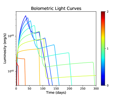
Figure 1: Type IIn SN model varying the CSM shape from a shell-like profile ($s=0$, blue) to a wind-like profile ($s=2$, red). We set the other model parameters to the following: SN ejecta mass $M_{\mathrm{ej}}=12M_{\odot}$, SN ejecta velocity $v_{\mathrm{ej}}=5000$ km s^-1, ejecta index $n=12$, CSM mass $M_{\mathrm{CSM}}=1M_{\odot}$ , CSM inner radius $R_{0}=10^{14}$ cm, CSM inner density $\rho_{CSM}(R_{0})=10^{-13}$ and CSM/ejecta opacity $\kappa=0.34$ cm² g^-1.

References

- Chatzopoulos et al. (2013) Chatzopoulos, E., Wheeler, J. C., Vinkó, J., Horvath, Z., & Nagy, A. 2013, The Astrophysical Journal, 773, 76
- Chevalier (1982) Chevalier, R. A. 1982, The Astrophysical Journal, 258, 790
- Filippenko (1997) Filippenko, A. V. 1997, Annual Review of Astronomy and Astrophysics, 35, 309
- Guillochon et al. (2018) Guillochon, J., Nicholl, M., Villar, V. A., et al. 2018, The Astrophysical Journal Supplement Series, 236, 6
- Hunter (2007) Hunter, J. D. 2007, Computing in Science & Engineering, 9, 90
- Moriya et al. (2013) Moriya, T. J., Maeda, K., Taddia, F., et al. 2013, Monthly Notices of the Royal Astronomical Society, 435, 1520
- Ofek et al. (2014) Ofek, E. O., Arcavi, I., Tal, D., et al. 2014, The Astrophysical Journal, 788, 154
- Oliphant (2006–) Oliphant, T. 2006–, NumPy: A guide to NumPy, USA: Trelgol Publishing, , , [Online; accessed ¡today¿]. http://www.numpy.org/
- Parker (1963) Parker, E. N. 1963, New York, Interscience Publishers, 1963.
- Smith & McCray (2007) Smith, N., & McCray, R. 2007, The Astrophysical Journal Letters, 671, L17
- Villar et al. (2017) Villar, V. A., Berger, E., Metzger, B. D., & Guillochon, J. 2017, The Astrophysical Journal, 849, 70
- Virtanen et al. (2019) Virtanen, P., Gommers, R., Oliphant, T. E., et al. 2019, arXiv e-prints, arXiv:1907.10121