Is the local Lorentz invariance of general relativity implemented by gauge bosons that have their own Yang-Mills-like action?

Abstract

General relativity with fermions has two independent symmetries: general coordinate invariance and local Lorentz invariance. General coordinate invariance is implemented by the Levi-Civita connection and by Cartan’s tetrads both of which have as their action the Einstein-Hilbert action. It is suggested here that local Lorentz invariance is implemented not by a combination of the Levi-Civita connection and Cartan’s tetrads known as the spin connection, but by independent Lorentz bosons $L^{ab}_{\phantom{ab}i}$ that gauge the Lorentz group, that couple to fermions like Yang-Mills fields, and that have their own Yang-Mills-like action. A nonsingular $4\times 4$ hermitian scalar field $h$ is needed to make the action of the Lorentz bosons invariant under local Lorentz transformations. Lorentz bosons couple to fermion number and generate a spin-dependent static potential that violates the weak equivalence principle. If a Higgs mechanism makes them massive, then the static potential also violates the inverse-square law. Experiments put upper bounds on the strength of such a potential for masses $m_{L}<20$ eV. These upper limits imply that Lorentz bosons, if they exist, are nearly stable and contribute to dark matter.

I Introduction

General relativity with fermions has two independent symmetries: general coordinate invariance and local Lorentz invariance. General coordinate invariance is the well-known, defining symmetry of general relativity. It acts on coordinates and on the world indexes of tensors but leaves Dirac and Lorentz indexes unchanged. It is implemented by the Levi-Civita connection and by Cartan’s tetrads.

Local Lorentz invariance is a quite different symmetry. It acts on Dirac and Lorentz indexes but leaves coordinates and world indexes unchanged. In standard formulations [1, 2, 3, 4, 5], the derivative of a Dirac field is made covariant $\left(\partial_{i}+\omega_{i}\right)\psi$ by a combination of the Levi-Civita connection $\Gamma^{j}_{\phantom{j}ki}$ and Cartan’s tetrads $c^{a}_{\phantom{a}j}$ known as the spin connection

$$\omega_{i}={}{\textstyle{\frac{1}{8}}}\,\omega^{ab}_{\phantom{ab}i}\,\bm{[}\gamma_{a},\gamma_{b}\bm{]}$$ (1)

in which

$$\omega^{ab}_{\phantom{ab}i}={}c^{a}_{\phantom{a}j}\,c^{bk}\,\Gamma^{j}_{\phantom{j}ki}+c^{a}_{\phantom{a}k}\,\partial_{i}c^{bk},$$ (2)

$a$ and $b$ are Lorentz indexes, and $i,j,k$ are world indexes.

Because it acts on Lorentz and Dirac indexes but leaves world indexes and coordinates unchanged, local Lorentz invariance is more like an internal symmetry than like general coordinate invariance. In theories with local Lorentz invariance and internal symmetry, the covariant derivative $D_{i}$ of a vector of Dirac fields $\psi$ has the spin connection $\omega_{i}$ and a matrix $A_{i}$ of Yang-Mills fields side by side

$$D_{i}\psi={}\left(\partial_{i}+\omega_{i}+A_{i}\right)\psi.$$ (3)

Just as the Yang-Mills connection $A_{i}$ is a linear combination $A_{i}={}-it^{\alpha}A^{\alpha}_{i}$ of the matrices $t^{\alpha}$ that generate the internal symmetry group, so too the spin connection $\omega_{i}$ is a linear combination $\omega_{i}={}{\textstyle{\frac{1}{8}}}\omega^{ab}_{\phantom{ab}i}\,\bm{[}\gamma_{a},\gamma_{b}\bm{]}$ of the matrices ${}-i{\textstyle{\frac{1}{4}}}\bm{[}\gamma_{a},\gamma_{b}\bm{]}$ that generate the Lorentz group.

So I ask: Does the independent symmetry of local Lorentz invariance have its own, independent gauge field

$$L_{i}={}{\textstyle{\frac{1}{8}}}\,L^{ab}_{\phantom{ab}i}\,\bm{[}\gamma_{a},\gamma_{b}\bm{]}$$ (4)

with its own field strength $F_{ik}={}\bm{[}\partial_{i}+L_{i},\partial_{k}+L_{k}\bm{]}$ and Yang-Mills-like action

$$S_{L}={}-\frac{1}{4f^{2}}\int{\rm Tr}\left(F^{\dagger}_{ik}\,h\,F^{ik}\,h^{-1}\right)\sqrt{g}\,d^{4}x?$$ (5)

This action is made suitably positive and invariant under the local Lorentz transformations

$$F^{\prime}={}D^{-1}(\Lambda)FD(\Lambda)\quad\mbox{and}\quad h^{\prime}={}D^{{\dagger}}(\Lambda)hD(\Lambda)$$ (6)

by a nonsingular $4\times 4$ hermitian scalar field $h$ [6, *Cahill:1979qt, *Cahill:1980, *Cahill:1981rq] whose action density is

$$S_{h}={}-M^{2}{\rm Tr}\big{[}(D_{i}h)h^{-1}(D^{i}h)h^{-1}\big{]}$$ (7)

in which its covariant derivative is [6, *Cahill:1979qt, *Cahill:1980, *Cahill:1981rq]

$$D_{i}h={}\partial_{i}h-hL_{i}-L_{i}^{\dagger}h.$$ (8)

The covariant derivative of a Dirac field would then be

$$D_{i}\psi={}\left(\partial_{i}+{\textstyle{\frac{1}{8}}}\,L^{ab}_{\phantom{ab}i}\,\bm{[}\gamma_{a},\gamma_{b}\bm{]}\right)\psi$$ (9)

instead of the standard form (1–3)

$$D_{i}\psi=\Big{(}\partial_{i}\,+\,{\textstyle{\frac{1}{8}}}\big{(}c^{a}_{\phantom{a}j}\,c^{bk}\,\Gamma^{j}_{\phantom{j}ki}+c^{a}_{\phantom{a}k}\,\partial_{i}c^{bk}\big{)}\bm{[}\gamma_{a},\gamma_{b}\bm{]}\Big{)}\psi.$$ (10)

If so, then the Lorentz bosons $L^{ab}_{\phantom{ab}i}$ couple to fermion number and not to mass and lead to Coulomb and Yukawa potentials that violate the inverse-square law and the weak equivalence principle. The hermitian scalar field $h$ must assume a nonzero value in the vacuum $h_{0}={}\langle 0|h|0\rangle$ because it is a nonsingular matrix. It may play the role of a new Higgs field. Its action (7) introduces a new mass into the theory.

Experiments [10, 11, 12, 13, 14, 15, 16, 12, 17, 18, 19, 20, 21, 22, 23, 12, 24, 25, 26, 27, 24, 28, 29, 30, 11, 23, 18, 22, 31, 32, 15, 33] have set upper limits on the strength of such Yukawa potentials for Lorentz bosons of mass less than $20\,$eV. These upper limits imply that Lorentz bosons, if they exist, are nearly stable and contribute to dark matter. Whether fermions couple to Lorentz bosons $L_{i}$ with their own action $S_{L}$ or to the spin connection $\omega_{i}$ is an open experimental question.

This paper outlines a version of general relativity with fermions in which the six vector bosons of the spin connection $\omega^{ab}_{\phantom{ab}i}$ are replaced by six vector bosons $L^{ab}_{\phantom{ab}i}$ that gauge the Lorentz group and have their own Yang-Mills-like action. The theory is invariant under general coordinate transformations and independently under local Lorentz transformations.

Section II sketches the traditional way of including fermions in a theory of general relativity. Section III describes the local Lorentz invariance of a theory with Lorentz bosons. Section IV says why general-coordinate invariance and local-Lorentz invariance are independent symmetries. Section V describes the Yang-Mills-like action (5) of the gauge fields $L^{ab}_{\phantom{ab}i}$ of the local Lorentz group. Sections VI and VII suggest ways to make gauge theory and general relativity more similar to each other. Section VIII discusses Higgs mechanisms that may give masses to the gauge bosons $L^{ab}_{\phantom{ab}i}$ of the Lorentz group. Section IX describes some of the constraints that experimental tests [10, 11, 12, 13, 14, 15, 16, 12, 17, 18, 19, 20, 21, 22, 23, 12, 24, 25, 26, 27, 24, 28, 29, 30, 11, 23, 18, 22, 31, 32, 15, 33] of the inverse-square law and of the weak equivalence principle place upon the proposed theory. Section X discusses the stability and masses of $L$ bosons and suggests that they may be part or all of dark matter. Section XI summarizes the paper.

II General relativity with fermions

A century ago, Einstein described gravity by the action

$$S_{E}={}\frac{1}{16\pi G}\int\!R\,\sqrt{g}\,\,d^{4}x={}\frac{1}{16\pi G}\int\!g^{ik}\,R_{ik}\,\sqrt{g}\,\,d^{4}x$$ (11)

in which $G={}1/m_{\text{P}}^{2}$ is Newton’s constant, the metric is $(-,+,+,+)$, letters from the middle of the alphabet are world indexes, $g=|\det g_{ik}|$ is the absolute value of the determinant of the space-time metric, and the Ricci tensor $R_{ik}={}R^{\ell}_{\phantom{\ell}i\ell k}$ is the trace of the Riemann tensor

$$R^{j}_{\phantom{j}i\ell k}={}\partial_{\ell}\Gamma^{j}_{\phantom{j}ki}-\partial_{k}\Gamma^{j}_{\phantom{j}\ell i}+\Gamma^{j}_{\phantom{j}\ell m}\,\Gamma^{m}_{\phantom{m}ki}-\Gamma^{j}_{\phantom{j}km}\,\Gamma^{m}_{\phantom{m}\ell i}$$ (12)

in which

$$\Gamma^{k}_{\phantom{k}i\ell}={}{\textstyle{\frac{1}{2}}}\,g^{kj}\left(\partial_{\ell}g_{ji}+\partial_{i}g_{j\ell}-\partial_{j}g_{i\ell}\right)=\Gamma^{k}_{\phantom{k}\ell i}$$ (13)

is the Levi-Civita connection which makes the covariant derivative of the metric vanish [34].

The standard action of general relativity with fermions is the sum of the Einstein-Hilbert action (11) and the action of matter fields including the Dirac action

$$\int-\bar{\psi}\gamma^{a}c^{i}_{a}\left(\partial_{i}+\omega_{i}+A_{i}\right)\psi\,\sqrt{g}\,d^{4}x.$$ (14)

In what follows, it is proposed to replace the spin connection $\omega_{i}$ in the standard Dirac action (14) with an independent gauge field $L_{i}={}-{\textstyle{\frac{1}{8}}}\,L^{ab}_{\phantom{ab}i}\,\bm{[}\gamma_{a},\gamma_{b}\bm{]}$ that has its own action (5) and to use

$$S_{D}={} \int-\bar{\psi}\,\gamma^{a}c^{i}_{a}\left(\partial_{i}+L_{i}+A_{i}\right)\psi\,\sqrt{g}\,d^{4}x$$ (15)

as the action of a Dirac field. This change reflects the independence of general coordinate invariance and local Lorentz invariance and makes general relativity and quantum field theory somewhat more similar.

III Local Lorentz Invariance

The Einstein action (11) has a trivial symmetry under local Lorentz transformations that act on Lorentz indexes but leave world indexes and coordinates unchanged. This symmetry becomes apparent when Cartan’s tetrads $c^{a}_{\phantom{a}i}$ and $c_{\phantom{b}k}^{b}$ are used to write the metric $g_{ik}$ in a form

$$g_{ik}(x)={}c^{a}_{\phantom{a}i}(x)\,\eta_{ab}\,c_{\phantom{b}k}^{b}(x)$$ (16)

that is unchanged by local Lorentz transformations

$$c^{\prime a}_{\phantom{{}^{\prime}a}i}(x)={}\Lambda^{a}_{\phantom{a}b}(x)\,c_{\phantom{b}i}^{b}(x).$$ (17)

The Levi-Civita connection (13) and the action (11) are defined in terms of the metric and so are also invariant under local Lorentz transformations.

More importantly, the two Dirac actions (14) and (15) have a nontrivial symmetry under local Lorentz transformations. Under such a local Lorentz transformation, a Dirac field transforms under the $({\textstyle{\frac{1}{2}}},0)\oplus(0,{\textstyle{\frac{1}{2}}})$ representation $D(\Lambda)$ of the Lorentz group with no change in its coordinates $x$

$$\psi^{\prime}_{\alpha}(x)={}D^{-1}_{\alpha\beta}(\Lambda(x))\,\psi_{\beta}(x).$$ (18)

The Lorentz-boson matrix $L_{i}={}-{\textstyle{\frac{1}{8}}}\,L^{ab}_{\phantom{ab}i}\,\bm{[}\gamma_{a},\gamma_{b}\bm{]}$ makes $\partial_{i}+L_{i}$ a covariant derivative

$$\partial_{i}+L^{\prime}_{i}={}D^{-1}(\Lambda)(\partial_{i}+L_{i})D(\Lambda).$$ (19)

In more detail with $\Lambda=\Lambda(x)$, the matrix $L_{i}$ transforms as

$$L^{\prime}_{i}={} D^{-1}(\Lambda)\,\partial_{i}D(\Lambda)+D^{-1}(\Lambda)\,L_{i}\,D(\Lambda)$$

$$={} D^{-1}(\Lambda)\,\partial_{i}D(\Lambda)-{\textstyle{\frac{1}{8}}}\,D^{-1}(\Lambda)\,L^{ab}_{\phantom{ab}i}\,\bm{[}\gamma_{a},\gamma_{b}\bm{]}\,D(\Lambda)$$

$$={} D^{-1}(\Lambda)\,\partial_{i}D(\Lambda)-{\textstyle{\frac{1}{8}}}\,L^{ab}_{\phantom{ab}i}\,\Lambda_{a}^{\phantom{a}c}\Lambda_{b}^{\phantom{b}d}\,\bm{[}\gamma_{c},\gamma_{d}\bm{]}$$ (20)

in which $\Lambda_{a}^{\phantom{a}c}=\Lambda^{-1c}_{\phantom{-1c}a}$. Since

$${\rm Tr}\left(\bm{[}\gamma^{a},\gamma^{b}\bm{]}\bm{[}\gamma_{c},\gamma_{d}\bm{]}\right)={}16\left(\delta^{a}_{d}\delta^{b}_{c}-\delta^{a}_{c}\delta^{b}_{d}\right),$$ (21)

its components transform as

$$L^{\prime ab}_{\phantom{ab}i}={} -{\textstyle{\frac{1}{2}}}\,{\rm Tr}(L^{\prime}_{i}\bm{[}\gamma^{a},\gamma^{b}\bm{]})$$ (22)

$$={} \Lambda_{c}^{\phantom{c}a}\Lambda_{d}^{\phantom{d}b}L^{cd}_{\phantom{cd}i}-{\textstyle{\frac{1}{2}}}\,{\rm Tr}\left(D^{-1}(\Lambda)\partial_{i}D(\Lambda)\bm{[}\gamma^{a},\gamma^{b}\bm{]}\right).$$

Under an infinitesimal transformation

$$\Lambda=I+\lambda\quad\mbox{and}\quad D(\lambda)=I-{\textstyle{\frac{1}{8}}}\lambda_{ab}\bm{[}\gamma^{a},\gamma^{b}\bm{]},$$ (23)

the Lorentz bosons transform as

$$L^{\prime ab}_{\phantom{ab}i}={}L^{ab}_{\phantom{ab}i}+L^{cb}_{\phantom{cb}i}\lambda_{c}^{\phantom{c}a}+L^{ad}_{\phantom{ad}i}\lambda_{d}^{\phantom{d}b}+\partial_{i}\lambda^{ab}.$$ (24)

The components of the spin connection obey similar equations, and the conventional Dirac action (14) also is invariant under local Lorentz transformations.

Local Lorentz transformations operate on the Lorentz indexes $a,b,c,\dots$ of the tetrads, of the spin connection $\omega^{ab}_{\phantom{ab}i}$, and of the gamma matrices $\gamma^{a}\bm{[}\gamma_{b},\gamma_{c}\bm{]}$, and also on the Dirac indexes $\alpha,\beta,\gamma$ of the gamma matrices and of the Dirac fields $\bar{\psi},\psi$, but not upon the world index $i$ or the spacetime coordinates $x$. In this sense, the invariance of Dirac’s action $S_{D}$ under local Lorentz transformations is like an internal symmetry.

IV Local Lorentz Invariance and Invariance Under General Coordinate Transformations Are Independent Symmetries

The Dirac action $S_{D}$ is invariant both under a local Lorentz transformation $\Lambda(x)$ and under a general coordinate transformation $x\to x^{\prime}$. Under a local Lorentz transformation $\Lambda(x)$, the coordinates are unchanged, $x^{\prime}=x$, and the fields transform as

$$\psi^{\prime}_{\alpha}(x)={} D^{-1}_{\alpha\beta}(\Lambda(x))\,\psi_{\beta}(x)$$

$$c^{\prime a}_{\phantom{{}^{\prime}a}i}(x)={} \Lambda^{a}_{\phantom{i}b}(x)\,c^{b}_{\phantom{b}i}(x)$$

$$L^{\prime ab}_{\phantom{{}^{\prime}ab}i}(x)={} \Lambda_{c}^{\phantom{c}a}(x)\Lambda_{d}^{\phantom{d}b}(x)L^{cd}_{\phantom{cd}i}(x)$$

$$-{} {\textstyle{\frac{1}{2}}}{\rm Tr}\left(D^{-1}(\Lambda(x))\partial_{i}D(\Lambda(x))\bm{[}\gamma^{a},\gamma^{b}\bm{]}\right)$$

$$h^{\prime}(x)={} D^{\dagger}(\Lambda(x))h(x)D(\Lambda(x))$$ (25)

in which $\Lambda_{c}^{\phantom{c}a}(x)={}\Lambda^{-1a}_{\phantom{-1a}c}$. Under a general coordinate transformation, the fields transform as

$$\psi^{\prime}_{\alpha}(x^{\prime})={} \psi_{\alpha}(x)$$

$$c^{\prime a}_{\phantom{{}^{\prime}a}i}(x^{\prime})={} \frac{\partial x^{k}}{\partial x^{\prime i}}\,c^{a}_{\phantom{b}k}(x)$$

$$L^{\prime ab}_{\phantom{ab}i}(x^{\prime})={} \frac{\partial x^{k}}{\partial x^{\prime i}}\,L^{ab}_{\phantom{ab}k}(x)$$

$$h(x^{\prime})={} h(x).$$ (26)

The two transformations, $\psi_{\alpha}(x)\to D^{-1}_{\alpha\beta}(\Lambda(x))\,\psi_{\beta}(x)$ and $x\to x^{\prime}$, are different and independent; the coordinates $x^{\prime}$ and $\Lambda(x)x$ are unrelated.

Every conventional, local Lorentz transformation is a general coordinate transformation, so one might be tempted to imagine that every general coordinate transformation is a conventional, local Lorentz transformation. But one can see that this is not the case by comparing the infinitesimal form of a general coordinate transformation

$$dx^{\prime i}={}\frac{\partial x^{\prime i}}{\partial x^{k}}\,dx^{k}$$ (27)

which has 16 generators with that of a conventional, local Lorentz transformation

$$dx^{\prime a}={}\Lambda^{a}_{\phantom{a}b}\,dx^{b}=dx^{a}+(\bm{\epsilon}_{r}\cdot\bm{R}^{a}_{\phantom{a}b}+\bm{\epsilon}_{b}\cdot\bm{B}^{a}_{\phantom{a}b})\,dx^{b}$$ (28)

which has only 6 [35].

Special relativity offers another temptation. In special relativity, global Lorentz transformations $\Lambda$ act on the spacetime coordinates and on the indexes of a Dirac field

$$\begin{split}x^{\prime a}={}&\Lambda^{a}_{\phantom{a}b}x^{b}\\ \psi^{\prime}_{\alpha}(x^{\prime})={}&D^{-1}_{\alpha\beta}(\Lambda)\,\psi_{\beta}(\Lambda x).\end{split}$$ (29)

This global Lorentz transformation leaves the specially relativistic Dirac action density unchanged

$$\big{[}-i\psi^{\dagger}\gamma^{0}\gamma^{a}\partial_{a}\psi\big{]}^{\prime}={} -i\psi^{\dagger}D^{-1{\dagger}}\gamma^{0}\gamma^{a}D^{-1}\partial^{\prime}_{a}\psi$$

$$={} -i\psi^{\dagger}\gamma^{0}D\gamma^{a}D^{-1}\Lambda_{a}^{\phantom{a}c}\partial_{c}\psi$$

$$={} -i\psi^{\dagger}\gamma^{0}\gamma^{b}\Lambda_{b}^{\phantom{b}a}\Lambda_{a}^{\phantom{a}c}\partial_{c}\psi$$ (30)

$$={} -i\psi^{\dagger}\gamma^{0}\gamma^{b}\delta^{c}_{b}\partial_{c}\psi=-i\psi^{\dagger}\gamma^{0}\gamma^{b}\partial_{b}\psi.$$

But in general relativity with fermions, Cartan’s tetrads $c_{a}^{i}$ allow the action to be invariant under a local Lorentz transformation without a corresponding general coordinate transformation. The matrix $D^{-1}_{\alpha\beta}(\Lambda(x))$ represents a local Lorentz transformation and acts (18) on the spinor indexes of the Dirac field but not on its spacetime coordinates. Since

$$D\gamma^{a}D^{-1}={}\Lambda_{a^{\prime}}^{\phantom{a^{\prime}}a}\gamma^{a^{\prime}}\quad\mbox{and}\quad D\gamma_{a}D^{-1}={}\Lambda^{a^{\prime}}_{\phantom{a^{\prime}}a}\gamma_{a^{\prime}},$$ (31)

a local Lorentz transformation (III) does not change

$$D\gamma^{a}D^{-1}c^{\prime i}_{a}=\gamma^{b}\Lambda_{b}^{\phantom{b}a}\Lambda_{a}^{\phantom{a}c}c_{c}^{i}=\gamma^{b}\delta^{c}_{b}c_{c}^{i}=\gamma^{b}c_{b}^{i}.$$ (32)

But the effect of a local Lorentz transformation (III) on the Lorentz matrix $L_{i}$ is

$$D(\partial_{i}+L^{\prime}_{i})D^{-1} -\partial_{i}={}-{\textstyle{\frac{1}{8}}}L^{\prime ab}_{\phantom{{}^{\prime}ab}i}\,D\bm{[}\gamma_{a},\gamma_{b}\bm{]}D^{-1}$$

$$={} -{\textstyle{\frac{1}{8}}}\Lambda^{\phantom{c}a}_{c}\Lambda^{\phantom{d}b}_{d}L^{cd}_{\phantom{ab}i}\,D\bm{[}\gamma_{a},\gamma_{b}\bm{]}D^{-1}$$

$$={} -{\textstyle{\frac{1}{8}}}\Lambda^{-1a}_{\phantom{-1a}c}\Lambda^{-1b}_{\phantom{-1b}d}L^{cd}_{\phantom{ab}i}\Lambda^{e}_{\phantom{a}a}\Lambda^{f}_{\phantom{a}b}\bm{[}\gamma_{e},\gamma_{f}\bm{]}$$

$$={} -{\textstyle{\frac{1}{8}}}\delta^{e}_{\phantom{e}c}\delta^{f}_{\phantom{f}d}L^{cd}_{\phantom{ab}i}\bm{[}\gamma_{e},\gamma_{f}\bm{]}$$

$$={} -{\textstyle{\frac{1}{8}}}L^{cd}_{\phantom{ab}i}\,\bm{[}\gamma_{c},\gamma_{d}\bm{]}=L_{i}$$ (33)

so that

$$D(\partial_{i}+L^{\prime}_{i})D^{-1}={}\partial_{i}+L_{i}.$$ (34)

A local Lorentz transformation therefore leaves the Dirac action density invariant

$$\big{[}-i\psi^{\dagger} \gamma^{0}\gamma^{a}c^{i}_{a}\left(\partial_{i}+L_{i}\right)\psi\big{]}^{\prime}$$

$$={} -i\psi^{\dagger}D^{-1{\dagger}}\gamma^{0}\gamma^{a}c^{\prime i}_{a}\left(\partial_{i}+L^{\prime}_{i}\right)D^{-1}\psi$$

$$={} -i\psi^{\dagger}D^{-1{\dagger}}\gamma^{0}\gamma^{a}c^{\prime i}_{a}D^{-1}D\left(\partial_{i}+L^{\prime}_{i}\right)D^{-1}\psi$$

$$={} -i\psi^{\dagger}\gamma^{0}D\gamma^{a}c^{\prime i}_{a}D^{-1}\!\left(\partial_{i}+L_{i}\right)\psi$$ (35)

$$={} -i\psi^{\dagger}\gamma^{0}\gamma^{a}c^{i}_{a}\left(\partial_{i}+L_{i}\right)\psi.$$

The symmetry under local Lorentz transformations is independent of the symmetry under general coordinate transformations. They are independent symmetries.

V Action of the Gauge Fields $L_{i}$

Since local Lorentz symmetry is like an internal symmetry, its gauge fields $L_{i}={}{\textstyle{\frac{1}{8}}}L^{ab}_{\phantom{ab}i}\,\bm{[}\gamma_{a},\gamma_{b}\bm{]}$ should have an action like that of a Yang-Mills field

$$S_{L}={}-\frac{1}{4f^{2}}\int{\rm Tr}\left(F^{\dagger}_{ik}\,{h}\,F^{ik}\,{h^{-1}}\right)\sqrt{g}\,d^{4}x$$ (36)

in which

$$F_{ik}={}\bm{[}\partial_{i}+L_{i},\partial_{k}+L_{k}\bm{]},$$ (37)

and $h$ is a $4\times 4$ nonsingular hermitian matrix [6, *Cahill:1979qt, *Cahill:1980, *Cahill:1981rq] . Under local Lorentz transformations $D(\Lambda(x))$, the field strengths $F^{ik}$ and the matrix $h$ transform as

$$\begin{split}F^{\prime ik}(x)={}&D^{-1}(\Lambda(x))F^{ik}(x)D(\Lambda(x))\\ h^{\prime}(x)={}&D^{\dagger}(\Lambda(x))h(x)D(\Lambda(x))\end{split}$$ (38)

and so the action $S_{L}$ is invariant under local Lorentz transformations as well as under general coordinate transformations [6, *Cahill:1979qt, *Cahill:1980, *Cahill:1981rq] .

One might think that it would be sufficient to set $h=\beta=i\gamma^{0}$, since $D^{\dagger}(\Lambda)\beta D(\Lambda)={}\beta$ and $D(\Lambda)\beta D^{\dagger}(\Lambda)=\beta$, but the resulting action $S_{L}$ is not bounded below.

In terms of the gamma matrices

$$\begin{split}\gamma^{0}={}&-i\,\begin{pmatrix}0&1\\ 1&0\\ \end{pmatrix},\quad\gamma^{i}=-i\,\begin{pmatrix}0&\sigma^{i}\\ {}-\sigma^{i}&0\\ \end{pmatrix},\\ {}&\quad\mbox{and}\quad\gamma^{5}=\begin{pmatrix}1&0\\ 0&-1\\ \end{pmatrix},\end{split}$$ (39)

the commutators in $L_{i}={}-{\textstyle{\frac{1}{8}}}L^{ab}_{\phantom{ab}i}\,\bm{[}\gamma_{a},\gamma_{b}\bm{]}$ are for spatial $a,b,c=1,2,3$,

$$\bm{[}\gamma_{a},\gamma_{b}\bm{]}=2i\epsilon_{abc}\sigma^{c}I\quad\mbox{and}\quad\bm{[}\gamma_{0},\gamma_{a}\bm{]}=-2\sigma^{a}\gamma^{5}.$$ (40)

So setting

$$\bm{r}^{a}_{\phantom{s}i}={}{\textstyle{\frac{1}{2}}}\epsilon_{abc}L^{bc}_{\phantom{bc}i}\quad\mbox{and}\quad\bm{b}^{a}_{\phantom{a}i}={}L^{a0}_{\phantom{a0}i},$$ (41)

the matrix of gauge fields $L_{i}$ is

$$L_{i}={} -{\textstyle{\frac{1}{8}}}\,L^{ab}_{\phantom{ab}i}\,\bm{[}\gamma_{a},\gamma_{b}\bm{]}=-i\,{\textstyle{\frac{1}{2}}}\,\bm{r}_{i}\cdot\bm{\sigma}\,I-{\textstyle{\frac{1}{2}}}\,\bm{b}_{i}\cdot\bm{\sigma}\,\gamma^{5},$$ (42)

and its field strength (37) is

$$F_{ik}={} \bm{[}\partial_{i}+L_{i},\partial_{k}+L_{k}\bm{]}$$ (43)

$$={} -i\,{\textstyle{\frac{1}{2}}}\,(\partial_{i}\bm{r}_{k}-\partial_{k}\bm{r}_{i}+\bm{r}_{i}\times\bm{r}_{k}-\bm{b}_{i}\times\bm{b}_{k})\cdot\bm{\sigma}\,I$$

$$-\,{\textstyle{\frac{1}{2}}}\,(\partial_{i}\bm{b}_{k}-\partial_{k}\bm{b}_{i}+\bm{r}_{i}\times\bm{b}_{k}+\bm{b}_{i}\times\bm{r}_{k})\cdot\bm{\sigma}\,\gamma^{5}.$$

With the abbreviations

$$\begin{split}\bm{R}_{ik}={}&(\partial_{i}\bm{r}_{k}-\partial_{k}\bm{r}_{i}+\bm{r}_{i}\times\bm{r}_{k}-\bm{b}_{i}\times\bm{b}_{k})\\ \bm{B}_{ik}=&(\partial_{i}\bm{b}_{k}-\partial_{k}\bm{b}_{i}+\bm{r}_{i}\times\bm{b}_{k}+\bm{b}_{i}\times\bm{r}_{k}),\end{split}$$ (44)

the action $S_{L}$ is the trace

$$\begin{split}S_{L}={}&-\frac{1}{16f^{2}}\int{\rm Tr}\Big{[}\big{(}\bm{R}_{ik}\cdot\bm{\sigma}I+i\bm{B}_{ik}\cdot\bm{\sigma}\gamma^{5}\big{)}h\\ {}&\qquad\big{(}\bm{R}^{ik}\cdot\bm{\sigma}I-i\bm{B}^{ik}\cdot\bm{\sigma}\gamma^{5}\big{)}h^{-1}\Big{]}\sqrt{g}\,d^{4}x.\end{split}$$ (45)

The $4\times 4$ nonsingular hermitian matrix $h$ may play a role in the action (15) of a spin-one-half field $\psi$ because we may take the quantity $\bar{\psi}$ either to be $\bar{\psi}=\psi^{\dagger}\beta$ as usual or to be $\bar{\psi}=\psi^{\dagger}h$ . The covariant derivative (8) of $h$ transforms as $\big{(}D_{i}h\big{)}^{\prime}={}D^{{\dagger}}(\Lambda)\,D_{i}h\,D(\Lambda)$ .

VI Making general relativity more similar to gauge theory

There are three reasons to define the covariant derivative of a Dirac field in terms of Lorentz bosons

$$L_{i}={}{\textstyle{\frac{1}{8}}}\,L^{ab}_{\phantom{ab}i}\,\bm{[}\gamma_{a},\gamma_{b}\bm{]}$$ (46)

with their own action (36) as

$$D_{i}\psi={}\left(\partial_{i}+L_{i}+A_{i}\right)\psi$$ (47)

rather than in terms of the spin connection (1)

$$\begin{split}\omega_{i}={}&{\textstyle{\frac{1}{8}}}\omega^{ab}_{\phantom{ab}i}\,\bm{[}\gamma_{a},\gamma_{b}\bm{]}\\ ={}&{\textstyle{\frac{1}{8}}}\left(c^{a}_{\phantom{a}j}\,c^{bk}\,\Gamma^{j}_{\phantom{j}ki}+c^{a}_{\phantom{a}k}\,\partial_{i}c^{bk}\right)\,\bm{[}\gamma_{a},\gamma_{b}\bm{]}\end{split}$$ (48)

as (3)

$$\left(\partial_{i}+\omega_{i}+A_{i}\right)\psi.$$ (49)

One reason is that the symmetry of local Lorentz transformations is independent of the symmetry of general coordinate transformations. So local Lorentz invariance should have its own gauge field $L_{i}$ and action $S_{L}$ independent of the tetrads and the Levi-Civita connection of general coordinate transformations.

A second reason to prefer the Lorentz connection $L_{i}$ to the spin connection $\omega_{i}$ is that the $L$-boson covariant derivative

$$\left(\partial_{i}+{\textstyle{\frac{1}{8}}}\,L^{ab}_{\phantom{ab}i}\,\bm{[}\gamma_{a},\gamma_{b}\bm{]}\right)\psi$$ (50)

is simpler than the spin-connection covariant derivative

$$\Big{(}\partial_{i}+{\textstyle{\frac{1}{8}}}{}(c^{a}_{\phantom{a}j}\,c^{bk}\,\Gamma^{j}_{\phantom{j}ki}+c^{a}_{\phantom{a}k}\,\partial_{i}c^{bk})\,\bm{[}\gamma_{a},\gamma_{b}\bm{]}\Big{)}\,\psi.$$ (51)

A third reason is that using the Lorentz connection (46), the Dirac covariant derivative (47), and the action (36) for the Lorentz connection, makes general relativity with fermions more similar to the gauge theories of the standard model.

VII Making gauge theory more similar to general relativity

Under a local Lorentz transformation, the spin connection $\omega_{i}$ changes more naturally, more automatically than does the Lorentz connection $L_{i}$. The automatic feature of the spin connection is that its definition (2) implies that under infinitesimal (23) and finite local Lorentz transformations it transforms as

$$\omega^{\prime ab}_{\phantom{{}^{\prime}ab}i}={}\omega^{ab}_{\phantom{ab}i}+\omega^{cb}_{\phantom{cb}i}\lambda_{c}^{\phantom{c}a}+\omega^{ad}_{\phantom{ad}i}\lambda_{d}^{\phantom{d}b}+\partial_{i}\lambda^{ab}$$ (52)

and as

$$\begin{split}\omega^{\prime ab}_{\phantom{{}^{\prime}ab}i}={}&\Lambda_{c}^{\phantom{c}a}\Lambda_{d}^{\phantom{d}b}\omega^{cd}_{\phantom{ab}i}+\Lambda^{\phantom{c}a}_{c}\partial_{i}\Lambda^{cb}.\end{split}$$ (53)

The terms $\partial_{i}\lambda^{ab}$ and $\Lambda^{\phantom{c}a}_{c}\partial_{i}\Lambda^{cb}$ occur automatically without the need to put in by hand a term like $D^{-1}(\Lambda)\partial_{i}D(\Lambda)$.

Terms like $D^{-1}(\Lambda)\,\partial_{i}D(\Lambda)$ are a common feature of gauge theories whether abelian or nonabelian. We can make them occur automatically in local Lorentz transformations if we add to the Lorentz connection $L^{ab}_{\phantom{{}^{\prime}ab}i}$ the term $u^{a}_{\phantom{a}\alpha}\,\partial_{i}\,u^{b\alpha}$ in which the four Lorentz 4-vectors $u^{a\alpha}(x)$ obey the condition

$$u^{a\alpha}\eta_{\alpha\beta}u^{b\beta}={}\eta^{ab},$$ (54)

and $\alpha=0,1,2,3$ is a label, not an index. It follows then from this condition (54) on the quartet of vectors $u^{a\alpha}$ that the augmented Lorentz connection $L^{ab}_{\text{new}\,i}$

$$L^{ab}_{\text{new}\,i}={}L^{ab}_{\phantom{cd}i}+u^{a}_{\phantom{a}\alpha}\,\partial_{i}\,u^{b\alpha}$$ (55)

automatically changes under a local Lorentz transformation $\Lambda_{c}^{\phantom{c}a}={}\Lambda^{-1a}_{\phantom{-1a}c}$ to

$$L^{\prime ab}_{\text{new}\,i}={} \Lambda_{c}^{\phantom{c}a}\Lambda_{d}^{\phantom{d}b}\,L^{cd}_{\phantom{cd}\,i}+\Lambda_{c}^{\phantom{c}a}u^{c}_{\phantom{a}\alpha}\,\partial_{i}\,(\Lambda_{d}^{\phantom{d}b}u^{d\alpha})$$

$$={} \Lambda_{c}^{\phantom{c}a}\Lambda_{d}^{\phantom{d}b}\,(L^{cd}_{\phantom{cd}\,i}+u^{c}_{\phantom{a}\alpha}\,\partial_{i}\,u^{d\alpha})+u^{c}_{\phantom{a}\alpha}u^{d\alpha}\Lambda_{c}^{\phantom{c}a}\,\partial_{i}\,\Lambda_{d}^{\phantom{d}b}$$

$$={} \Lambda_{c}^{\phantom{c}a}\Lambda_{d}^{\phantom{d}b}\,L^{cd}_{\text{new}\,i}+\eta^{cd}\Lambda_{c}^{\phantom{c}a}\,\partial_{i}\,\Lambda_{d}^{\phantom{d}b}$$

$$={} \Lambda_{c}^{\phantom{c}a}\Lambda_{d}^{\phantom{d}b}\,L^{cd}_{\text{new}\,i}+\Lambda_{c}^{\phantom{c}a}\,\partial_{i}\,\Lambda^{cb}$$

$$={} \Lambda_{c}^{\phantom{c}a}\Lambda_{d}^{\phantom{d}b}\,L^{cd}_{\text{new}\,i}+\Lambda^{-1a}_{\phantom{-1a}c}\,\partial_{i}\,\Lambda^{cb}$$ (56)

without the need to explicitly add the last term $\Lambda^{-1a}_{\phantom{-1a}c}\,\partial_{i}\,\Lambda^{cb}$ by hand.

In matrix form, the condition (54) is the requirement

$$u^{a\alpha}\eta_{\alpha\beta}u^{b\beta}={}\eta^{ab}$$ (57)

that the matrix formed by the quartet of vectors $u^{a\alpha}$ be a Lorentz transformation

$$x_{a}u^{a\alpha}\eta_{\alpha\beta}u^{b\beta}y_{b}={}x_{a}\eta^{ab}y_{b}.$$ (58)

The augmentation of the Lorentz connection $L^{ab}_{\phantom{ab}i}\to L^{ab}_{\text{new}\,i}$ by the addition of the term $u^{a}_{\phantom{a}\alpha}\,\partial_{i}\,u^{b\alpha}$, which is similar to the tetrad term $c^{a}_{\phantom{a}k}\,\partial_{i}c^{bk}$ of the spin connection (2), makes its change (56) under local Lorentz transformations as automatic as that (53) of the spin connection.

The use of a more automatic connection makes gauge theory more similar to general relativity with fermions.

We can extend the use of such terms to internal symmetries and so make the inhomogeneous terms appear automatically rather than by hand or by fiat. For instance, we can augment the abelian connection $A_{i}$ to

$$A_{\text{new}\,i}(x)={}A_{i}(x)+e^{-i\phi(x)}\partial_{i}e^{i\phi(x)}$$ (59)

in which $\phi(x)$ is an arbitrary phase. A $U(1)$ transformation

$$e^{-i\phi(x)}\to e^{-i(\theta(x)+\phi(x))}\,\,\,\text{and}\,\,\,\psi(x)\to e^{-i\theta(x)}\psi(x)$$ (60)

would then change the covariant derivative $(\partial_{i}+A_{\text{new}\,i})\psi$ to

$$[(\partial_{i}+ A_{\text{new}\,i})\psi]^{\prime}={}(\partial_{i}+A_{i}+e^{-i(\theta+\phi)}\partial_{i}e^{i(\theta+\phi)})e^{-i\theta}\psi$$

$$={} e^{-i\theta}(\partial_{i}-i\partial_{i}\theta+A_{i}+i\partial_{i}\theta+e^{-i\phi}\partial_{i}e^{i\phi})\psi$$ (61)

$$={} e^{-i\theta}(\partial_{i}+A_{i}+e^{-i\phi}\partial_{i}e^{i\phi})\psi=e^{-i\theta}(\partial_{i}+A_{\text{new}\,i})\psi.$$

Similarly, we can augment the nonabelian connection $A_{i}={}-it^{\alpha}A^{\alpha}_{i}$ for $SU(n)$ to

$$A_{\text{new}\,i}(x)={}A_{i}(x)+u_{\alpha\beta}(x)\partial_{i}u^{*}_{\alpha\gamma}(x)$$ (62)

in which the $n$ $n$-vectors $u_{\alpha\gamma}$ are orthonormal

$$u_{\beta\alpha}u^{*}_{\gamma\alpha}={}\delta_{\beta\gamma}.$$ (63)

An $SU(n)$ transformation

$$A_{i}\to gA_{i}g^{\dagger},\,\,\,u\to gu,\,\,\,\text{and}\,\,\,\psi\to g\psi$$ (64)

would then change the covariant derivative $(\partial_{i}+A_{\text{new}\,i})\psi$ to

$$[(\partial_{i}+ A_{\text{new}\,i})\psi]^{\prime}={}(\partial_{i}+gA_{i}g^{\dagger}+g\,u\,\partial_{i}(u^{\dagger}g^{\dagger}))g\psi$$

$$={} g(\partial_{i}+g^{\dagger}\partial_{i}g+A_{i}+(\partial_{i}g^{\dagger})uu^{\dagger}g+u\,\partial_{i}\,u^{\dagger})\psi$$

$$={} g(\partial_{i}+g^{\dagger}\partial_{i}g+A_{i}+(\partial_{i}g^{\dagger})g+u\,\partial_{i}\,u^{\dagger})\psi$$

$$={} g(\partial_{i}+A_{i}+u\,\partial_{i}\,u^{\dagger})\psi=g(\partial_{i}+A_{\text{new}\,i})\psi.$$ (65)

VIII Possible Higgs Mechanisms

The $4\times 4$ nonsingular hermitian matrix $h$ is needed to make the action (36) gauge invariant. It also may replace $\beta$ in the fermionic action (15). Since it is nonsingular, it must assume a nonzero average value in the vacuum

$$h_{0}={}\langle 0|h|0\rangle.$$ (66)

So we have a new kind of Higgs mechanism that can give masses to gauge fields and fermions. This will be taken up in later papers.

Other kinds of Higgs mechanisms are also possible with different Higgs fields. The actions $S_{L}$ and $S_{D}$ (5 & 15) leave the gauge bosons $L$ massless, but a Higgs mechanism is possible. An interaction with a field $v^{a}$ that is a scalar under general coordinate transformations but a vector under local Lorentz transformations has as its covariant derivative

$$D_{i}v^{a}={}\partial_{i}v^{a}+L^{a}_{\phantom{a}bi}v^{b}.$$ (67)

If the time component $v^{0}$ has a nonzero mean value in the vacuum $\langle 0|v^{0}|0\rangle\neq 0$, then the scalar $-{}D_{i}v^{a}D^{i}v_{a}$ contains a mass term

$${}-L^{a}_{\phantom{a}0i}v^{0}\,L_{a}^{\phantom{a}0i}v_{0}={}-L^{a0}_{\phantom{a0}i}v^{0}\,L^{a0i}v^{0}$$ (68)

that makes the boost vector bosons $b^{s}_{\phantom{s}i}={}L^{s0}_{\phantom{s0}i}$ massive but leaves the rotational vector bosons $r^{s}_{\phantom{s}i}={}{\textstyle{\frac{1}{2}}}\epsilon_{stu}L^{tu}_{\phantom{tu}i}$ massless. On the other hand, if the spatial components have a nonzero mean value, $\langle 0|\bm{v}|0\rangle\neq 0$, then the mass term is

$${}-L^{a}_{\phantom{a}si}v^{s}\,L_{a}^{\phantom{a}si}v_{s}={}-L^{s^{\prime}s}_{\phantom{s^{\prime}s}i}v^{s}\,L^{s^{\prime}si}v^{s}+L^{0s}_{\phantom{as}i}v^{s}\,L^{0si}v^{s}.$$ (69)

Adding the two mass terms (68 and 69), we find

$$\begin{split}{}-L^{a}_{\phantom{a}0i}v^{b}\,L_{a}^{\phantom{a}0i}v_{b}={}&L^{0s}_{\phantom{0s}i}v^{a}\,L^{0si}v_{a}-L^{s^{\prime}s}_{\phantom{s^{\prime}s}i}v^{s}\,L^{s^{\prime}si}v^{s}\end{split}$$ (70)

which makes all six gauge bosons massive as long as the mean value is timelike

$$\langle 0|v^{a}v_{a}|0\rangle<0$$ (71)

and at least two spatial components $\langle 0|v^{s}|0\rangle\neq 0$ have nonzero mean values in the vacuum. This condition holds in all Lorentz frames if three vectors $v^{a1},v^{a2},$ and $v^{a3}$ have different timelike mean values in the vacuum.

In the vacuum of flat space, tetrads have mean values that are Lorentz transforms of $c^{a}_{i}={}\delta^{a}_{i}$ and that produce the Minkowski metric (16)

$$g_{ik}={}\delta^{a}_{i}\,\eta_{ab}\,\delta^{b}_{k}=\eta_{ik}.$$ (72)

So it is tempting to look for a Higgs mechanism that uses the covariant derivatives $D_{\ell}\,c^{a}_{\phantom{i}k}$ of the tetrads. For $\Gamma^{j}_{\phantom{j}k\ell}=0$ and $c^{a}_{\phantom{a}k}=\delta^{a}_{k}$, the term

$$\begin{split}-{\textstyle{\frac{1}{2}}}\,m_{L}^{2}\,(D^{i}\,c_{a}^{\phantom{a}k})\,D_{i}\,c^{a}_{\phantom{a}k}={}&-{\textstyle{\frac{1}{2}}}\,m_{L}^{2}\,L_{a}^{\phantom{a}bi}\,c_{b}^{\phantom{b}k}\,\,L^{a}_{\phantom{a}ci}\,c^{c}_{\phantom{b}k}\\ ={}&-{\textstyle{\frac{1}{2}}}\,m_{L}^{2}\,L_{ab}^{\phantom{ab}i}\,L^{ab}_{\phantom{ab}i}\end{split}$$ (73)

makes the rotational bosons $\bm{r}^{s}_{\phantom{s}i}={\textstyle{\frac{1}{2}}}\epsilon_{stu}L^{tu}_{\phantom{tu}i}$ massive but makes the boost bosons $\bm{b}^{s}_{\phantom{s}i}={}L^{s0}_{\phantom{s0}i}$ tachyons. If weakly coupled tachyons are unacceptable, then the Higgs mechanism (67–70) that uses three world-scalar Lorentz vectors with different time-like mean values in the vacuum $v^{a}_{1}$, $v^{a}_{2}$, $v^{a}_{3}$ is a more plausible way to make the gauge bosons $L^{ab}_{\phantom{ab}i}$ massive.

IX Tests of the Inverse-Square Law

In the static limit, the exchange of six Lorentz bosons $L^{ab}_{\phantom{ab}i}$ of mass $m_{L}$ would imply that two macroscopic bodies of $F$ and $F^{\prime}$ fermions separated by a distance $r$ would contribute to the energy a static Yukawa potential

$$V_{L}(r)=\frac{3\,FF^{\prime}f^{2}}{2\pi r}\,e^{-m_{L}r}.$$ (74)

This potential is positive and repulsive (between fermions and between antifermions) because the $L$’s are vector bosons. It violates the weak equivalence principle because it depends upon the number $F$ of fermions (minus the number of antifermions) as $F=3B+L$ and not upon their masses. The potential $V_{L}(r)$ changes Newton’s potential to

$$V_{NL}(r)={}-G\,\frac{mm^{\prime}}{r}\left(1+\alpha\,e^{-r/\lambda}\right)$$ (75)

in which the coupling strength $\alpha$ is

$$\alpha={}-\frac{3FF^{\prime}f^{2}}{2\pi Gmm^{\prime}}={}-\frac{3FF^{\prime}m_{\text{P}}^{2}f^{2}}{2\pi mm^{\prime}},$$ (76)

and the length $\lambda$ is $\lambda=\hbar/cm_{L}$. Couplings $\alpha\sim 1$ are of gravitational strength. Experiments [10, 11, 12, 13, 14, 15, 16, 12, 17, 18, 19, 20, 21, 22, 23, 12, 24, 25, 26, 27, 24, 28, 29, 30, 11, 23, 18, 22, 31, 32, 15, 33] that test the inverse-square law and the weak equivalence principle have put upper limits on the strength $|\alpha|$ of the coupling for a wide range of lengths $10^{-8}<\lambda<10^{13}$ m and masses $2\times 10^{-20}<m_{L}<20$ eV.

Experiments that tested the inverse-square law at very short distances, between 10 nm and 3 mm, were done with masses of gold [10], of gold and silicon [11], of platinum [12], and of tungsten [13]. For a mass $m$ of $N$ atoms of gold which has $F_{\text{Au}}=670$ fermions (quarks and electrons) in each atom of mass $m_{\text{Au}}=196.966$ u, the ratio $Fm_{\text{P}}/m$ that appears in the coupling $\alpha$ (76) is

$$\frac{NF_{\text{Au}}\,m_{\text{P}}}{Nm_{\text{Au}}}={}\frac{F_{\text{Au}}\,m_{\text{P}}}{m_{\text{Au}}}={}\frac{670\,m_{\text{P}}}{196.966\,u}=4.458\times 10^{19}.$$ (77)

So the coupling strength is $\alpha_{\text{Au}}={}-9.490\times 10^{38}\,f^{2}$ for gold. An atom of silicon has $F_{\text{Si}}=98$ fermions and a mass of $m_{\text{Si}}=28.085$ u, so $F_{\text{Si}}\,m_{\text{P}}/m_{\text{Si}}=4.573$ and $\alpha_{\text{Si}}={}-9.988\times 10^{38}\,f^{2}$. Platinum has $F_{\text{Pt}}=663$ and $m_{\text{Pt}}=195.084\,u$, so $\alpha_{\text{Pt}}={}-9.474\times 10^{38}\,f^{2}$. Tungsten has $F_{\text{W}}=626$ and $m_{\text{W}}=183.84\,u$, so $\alpha_{\text{W}}={}-9.510\times 10^{38}\,f^{2}$. For such test masses, $f^{2}\approx|\alpha|\times 10^{-39}$.

The Riverside group [10] placed on the strength $|\alpha_{\text{Au}}|$ an upper limit (95% confidence) that drops from $|\alpha_{\text{Au}}|\lesssim 10^{19}$ to $|\alpha_{\text{Au}}|\lesssim 10^{16}$ as the length $\lambda$ rises from $10^{-8}$ m to $4\times 10^{-8}$ m. The IUPUI group [11] put an upper limit (95% confidence) on the strength $|\alpha_{\text{Au-Si}}|$ that drops from $|\alpha_{\text{Au-Si}}|\lesssim 10^{16}$ to $|\alpha_{\text{Au-Si}}|\lesssim 10^{5}$ as the length $\lambda$ rises from $4\times 10^{-8}$ m to $8\times 10^{-6}$ m. These results of the Riverside and IUIPUI groups are plotted in Fig. 1 from Chen et al. [11].

Other short-distance experiments [12, 13, 15, 16, 17, 18, 19, 20, 21, 22, 23, 24, 30, 23, 18, 22, 31, 32, 15] have tested the inverse-square law at the slightly longer distances of $2\times 10^{-6}<\lambda<3\times 10^{-3}$ m. The Washington group [12] used test masses of platinum. The  [13] used test masses of tungsten. The upper limits (95% confidence) on the strength $|\alpha|$ are shown for platinum in Fig. 2 from Lee et al. [12] and for tungsten in Fig. 3 from Tan et al. [13]. The upper limit on the strength $|\alpha|$ falls from $|\alpha|\lesssim 10^{6}$ at $\lambda\sim 2\times 10^{-6}$ m to $|\alpha|\lesssim 10^{4}$ at $\lambda\sim 8\times 10^{-6}$ m and then from $|\alpha|\lesssim 10^{3}$ at $\lambda\sim 10^{-5}$ m to $|\alpha|\lesssim 1$ at $\lambda\sim 4\times 10^{-5}$ m and to $|\alpha|\lesssim 10^{-3}$ at $\lambda\sim 2\times 10^{-3}$ m.

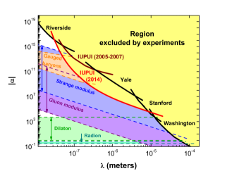
Figure 1: Upper limits (95% confidence) on the strength $|\alpha_{\text{Au}}|$ of Yukawa potentials that violate the inverse-square law at distances $10^{-8}<\lambda<2\times 10^{-4}$ m. (Fig. 4 of Chen et al. [11])

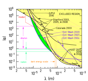
Figure 2: Upper limits (95% confidence) on the strength $|\alpha_{\text{Pt}}|$ of Yukawa potentials that violate the inverse-square law at sub-mm distances [12, 13, 14, 15, 16, 12, 17, 18, 19, 20, 21, 22, 23, 24]. (Fig. 5b of Lee et al. [12])

Figure 3: Upper limits (95% confidence) on the strength $|\alpha_{\text{W}}|$ of Yukawa potentials that violate the inverse-square law at mm and sub-mm distances [13, 21, 19, 24, 30, 11, 23, 18, 22, 31, 32, 15]. Light lines are theory [17, 26] (Fig. 6 of Tan et al. [13]).

Other groups [32, 17, 29, 25, 26, 27, 24, 28, 33] have tested the inverse-square law over a huge range of longer distances, $10^{-3}<\lambda<3\times 10^{15}$ m. In 2012 the HUST group [32] put an upper limit of $|\alpha|\lesssim 10^{-3}$ for $7\times 10^{-4}<\lambda<5\times 10^{-3}$ m, while in 1985 the Irvine group [24] put an upper limit of $|\alpha|\lesssim 10^{-3}$ for lengths $7\times 10^{-3}<\lambda<10^{-1}$ m.

Fischbach and Talmadge [33] and Adelberger et al. [17] have reported tests of the inverse-square law for distances in the range $10^{-2}<\lambda<10^{15}$ m [17, 27, 24, 28, 33]. As shown in Fig. 4 from Adelberger et al. [17],

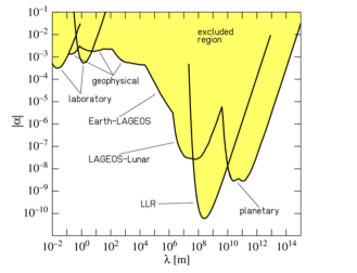
Figure 4: Upper limits (95% confidence) on the strength $|\alpha|$ of Yukawa violations of the inverse-square law at large distances $10^{-2}<\lambda<10^{15}$ m [27, 24, 28, 33, 17] (Fig. 10 of Adelberger et al. [17]).

the upper limit lies between $|\alpha|<3\times 10^{-4}$ and $|\alpha|<2\times 10^{-3}$ for $10^{-2}<\lambda<10^{4}$ m but drops from $|\alpha|\lesssim 10^{-4}$ to $|\alpha|\lesssim 10^{-10}$ as the length increases from $10^{4}$ to $10^{8}$ m. The upper limit is about $|\alpha|\lesssim 5\times 10^{-9}$ on planetary scales $10^{10}<\lambda<5\times 10^{11}$ m.

The Washington group have used torsion-balance experiments to look for Yukawa potentials that violate the weak equivalence principle in the range of distances $0.3<\lambda<10^{9}$ m [17]. They have put upper limits (95% confidence) on the strength $|\alpha|$ of the coupling to $B$, $Z$, and $N\equiv B-L$ but not explicitly on the coupling to fermion number $F=3B+L$. For $B$, their upper limit runs from $|\alpha|\lesssim 10^{-5}$ at $10^{-1}$ m to $|\alpha|\lesssim 6\times 10^{-8}$ at $7\times 10^{5}$ m and then falls to $|\alpha|\lesssim 10^{-10}$ for $10^{7}<\lambda<10^{13}$ m as shown by the dashed lines in Fig. 5 from Bergé et al. [14]. For $Z$ and $N$, their upper limit runs from $|\alpha|\lesssim 10^{-6}$ at $10^{-1}$ m to $|\alpha|\lesssim 6\times 10^{-9}$ at $10^{6}$ m and then falls to $|\alpha|\lesssim 2\times 10^{-11}$ for $10^{7}<\lambda<10^{9}$ m [17].

More recent satellite measurements by the MICROSCOPE mission have lowered the upper limit on the strength $|\alpha|$ of Yukawa potentials that violate the weak equivalence principle by about an order of magnitude for $10^{7}<\lambda<10^{9}$ m [14]. The upper limit for coupling to $B$ is $|\alpha|\lesssim 10^{-11}$ for $10^{7}<\lambda<10^{9}$ m as shown in Fig. 5 from Bergé et al. [14]. Their limit for coupling to $N$ is even lower: $|\alpha|\lesssim 4\times 10^{-13}$ for $10^{7}<\lambda<10^{9}$ m [14].

Figure 5: Upper limits (95% confidence) on the strength $|\alpha|$ of Yukawa potentials that violate the weak equivalence principle at long distances [14, 17, 25, 27, 24, 28] (Fig. 1 of Bergé et al. [14]).

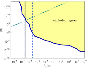
Figure 6: The upper bound (95% confidence) on the strength $|\alpha|$ of Yukawa potentials that violate the inverse-square law or the weak equivalence principle at various distances $\lambda$ is the solid dark-blue curve [10, 11, 12, 13, 14, 15, 16, 12, 17, 18, 19, 20, 21, 22, 23, 12, 24, 25, 26, 27, 24, 28, 29, 30, 11, 23, 18, 22, 31, 32, 15, 33]. The region under the dotted green line denotes $L$ bosons with lifetimes greater than the age of the universe for the case in which the fudge factor $b=1$. The region below that line and between the vertical dashed blue lines denotes $L$ bosons that are between 1 and 100% of dark matter. The thin vertical gray solid line marks the wavelength of an $L$ boson whose mass is $2\,m_{\nu_{e}}^{\text{eff}}={}2.2$ eV [36].

Some of these important results [10, 11, 12, 13, 14, 15, 16, 12, 17, 18, 19, 20, 21, 22, 23, 12, 24, 25, 26, 27, 24, 28, 29, 30, 11, 23, 18, 22, 31, 32, 15, 33] are summarized in broad-brush fashion in Fig. 6. The upper bound (95% confidence) on $|\alpha|$ is the solid dark-blue curve which falls from $10^{19}$ for $\lambda=7\times 10^{-8}$ m to $10^{-11}$ at $\lambda=10^{9}$ m. The $(\lambda,|\alpha|)$ region above this curve is excluded. Points in the allowed region that are below the blue-green dotted line correspond to $L$ bosons with lifetimes longer than the age of the universe. Those that also are between the vertical dashed lines denote effectively stable $L$ bosons whose masses could account for between 1 and 100% of dark matter.

X Lorentz bosons as dark matter

Analysis of the double galaxy cluster 1E0657-558 (the “bullet cluster” at $z=0.296$) suggests [37, 38] that dark matter interacts weakly, perhaps with gravitational strength $|\alpha|\sim 1$. As of now, there has been no accepted detection of dark matter in a laboratory.

The experiments [10, 11, 12, 13, 14, 15, 16, 12, 17, 18, 19, 20, 21, 22, 23, 12, 24, 25, 26, 27, 24, 28, 29, 30, 11, 23, 18, 22, 31, 32, 15, 33] sketched in Sec. IX put no upper limits on the mass $m_{L}=h/c\lambda$ of $L$ bosons and no lower limits on their coupling $|\alpha|$. The proposed $L$ bosons are electrically neutral. If their mass is heavy enough and if their coupling is sufficiently weak, then they would be an effectively stable part of dark matter.

Because they couple to fermion number and not to mass, their coupling $f^{2}$ is much weaker than $|\alpha|$ by a factor related to Avogadro’s number. For the metals (Au, Si, Pt, and W) used in many of the experiments [10, 11, 12, 13, 14, 15, 16, 12, 17, 18, 19, 20, 21, 22, 23, 12, 24, 25, 26, 27, 24, 28, 29, 30, 11, 23, 18, 22, 31, 32, 15], the relation is

$$f^{2}\sim|\alpha|\times 10^{-39}.$$ (78)

Even for the highest upper limit $|\alpha|<10^{19}$ shown in Fig. 6, the coupling of the $L$ bosons is only $f^{2}\lesssim 10^{-20}$.

Because they interact so weakly, $L$ bosons decay slowly. The decay width of the $Z$ boson is $\Gamma_{Z}=3.7\,e^{2}\,m_{Z}c^{2}/4\pi=2.5$ GeV, and its lifetime is $\tau_{Z}=\hbar/\Gamma_{Z}=2.6\times 10^{-25}$ s. The analog of the electromagnetic coupling $e^{2}/4\pi\sim 1/137$ for $L$ bosons is $f^{2}/4\pi$. In terms of $f^{2}$ and $|\alpha|$ (78), the decay width of an $L$ boson of mass $m_{L}$ is roughly

$$\Gamma_{L}\sim{}\frac{b\,f^{2}\,m_{L}c^{2}}{4\pi}=\frac{b\,|\alpha|\,m_{L}c^{2}}{4\pi}\times 10^{-39}$$ (79)

in which $b$ is a fudge factor, $0.1\lesssim b\lesssim 10$, that depends on the decay channels. The $L$ boson lifetime then is

$$\begin{split}\tau={}&\frac{\hbar}{\Gamma_{L}}=\frac{8.3\times 10^{24}}{b\,|\alpha|\,m_{L}c^{2}[\text{eV}]}\,\,\text{s}=\frac{1.9}{b|\alpha|}\,\frac{10^{7}}{m_{L}c^{2}[\text{eV}]}\,\,t_{0}\end{split}$$ (80)

in which $t_{0}=4.356\times 10^{17}$s is 13.8 billion years, the age of the universe. An $L$ boson of mass $m_{L}<(19/b|\alpha|)\,\text{MeV}$ is effectively stable in that its lifetime exceeds the age of the universe. If the fudge factor $b$ is taken to be unity, then $L$ bosons of wavelength $\lambda$ are effectively stable for couplings

$$|\alpha|\lesssim\left(1.5\times 10^{13}\right)\,\,\lambda\,[\text{m}]$$ (81)

which is the dotted green line in Fig. 6. Points below it denote effectively stable $L$ bosons.

If the lightest fermion has mass $m_{\text{lightest}}$, then $L$ bosons of mass less than $2\,m_{\text{lightest}}$ would be absolutely stable. The dash-dotted gray vertical line in Fig. 6 is the wavelength $\lambda=5.6\times 10^{-7}$m of twice the upper limit on the effective mass of the electron neutrino, $2\,m_{\nu_{e}}^{(\text{eff})}$ [36].

The mass density of cold dark matter is $\rho_{\text{cdm}}=(2.2414\pm 0.017)\times 10^{-27}$ kg m^-3 [39, col. 7, p. 15]. So if all of cold dark matter were made of $L$ bosons of mass $m_{L}$, then their number density would be

$$\begin{split}n_{L}={}&\frac{\rho_{\text{cdm}}}{m_{L}}={}\frac{1.26\times 10^{9}}{m_{L}c^{2}[\text{eV}]}\,\text{m}^{-3}.\end{split}$$ (82)

To estimate the present number density of each kind of $L$ boson, I’ll assume that the $L$ bosons are effectively stable and have not interacted since they dropped out of equilibrium in the very early universe.

At temperaures $kT\gg m_{L}c^{2}$ so high that the weakly interacting $L$ bosons were in thermal equilibrium, the number density of each of the six $L$ bosons is given by the Planck distribution as

$$n(T)={}\frac{3\zeta(3)(kT)^{3}}{\pi^{2}(\hbar c)^{3}}=\frac{9.609\times 10^{7}\,T^{3}}{(\text{m\,K})^{3}}.$$ (83)

In the limit of vanishing coupling $|\alpha|\to 0$, the number $n(t)a^{3}(t)$ of $L$ bosons within a fixed comoving box does not change with time. So the number now $n(t_{0})a^{3}(t_{0})=n(t_{0})$ is the number at any earlier time multiplied by $a^{3}(t)$

$$n(t_{0})=n(t)a^{3}(t).$$ (84)

At very early times, we may approximate the integral for the time as a function of the scale factor $a$ as [40]

$$t(a)={} \frac{1}{H_{0}}\int_{0}^{a}\!\!\frac{dx}{\sqrt{\Omega_{\Lambda}\,x^{2}+\Omega_{k}+\Omega_{m}\,x^{-1}+\Omega_{r}\,x^{-2}}}$$

$$\approx{} \frac{1}{H_{0}}\int_{0}^{a}\!\!\frac{x\,dx}{\sqrt{\Omega_{r}}}=\frac{a^{2}}{2H_{0}\sqrt{\Omega_{r}}}.$$ (85)

The Hubble constant and the fraction $\Omega_{r}=9.0824\times 10^{-5}$ then give us the scale-factor as

$$a(t)=\sqrt{2H_{0}\sqrt{\Omega_{r}}\,t}=2.04\times 10^{-10}\sqrt{t\text{[}s]}.$$ (86)

If $\mathcal{N}$ types of particles made up the radiation at very early times, then the time and the temperature were related by [41]

$$\sqrt{\mathcal{N}}\,\,t\,T^{2}={}\sqrt{\frac{3c^{2}}{16\pi Ga_{\text{r}}}}=3.25924\times 10^{20}\,\,\text{s\,K}^{2}$$ (87)

in which $a_{\text{r}}$ is the radiation constant

$$a_{\text{r}}={}\frac{\pi^{2}k^{4}}{15\hbar^{3}c^{3}}=7.56577(5)\times 10^{-16}\,\text{J m}^{-3}\,\text{K}^{-4}.$$ (88)

So in terms of the number density (83), the scale-factor (86), and the time-temperature relation (87), the number density is roughly

$$\begin{split}n(t_{0})={}n(t)a^{3}(t)=\frac{4.8\times 10^{9}}{\mathcal{N}^{3/4}}\,\text{m}^{-3}.\end{split}$$ (89)

In the standard model, $\mathcal{N}=126$, but the actual number relevant at high temperatures may be much higher. If we assume that $\mathcal{N}=4^{4}$, then $\mathcal{N}^{-3/4}=1/64$, and the present number density of each kind of $L$ boson would be

$$n(t_{0})=7.5\times 10^{7}\,\text{m}^{-3}.$$ (90)

Let us further assume that all six $L$ bosons get the same mass $m_{L}$. In this case, if their mass density is not to exceed the density of dark matter, then the inequality

$$6\,m_{L}\,n(t_{0})<\rho_{\text{cdm}}=2.24\times 10^{-27}\,\text{kg m}^{-3}$$ (91)

implies that the mass $m_{L}$ must be less than

$$\begin{split}m_{L}<4.9\times 10^{-36}\,\text{kg}={}&2.8\,\text{eV}/c^{2}.\end{split}$$ (92)

The lifetime of an $L$ boson (80) would then be

$$\tau_{L}>\frac{3.4}{b|\alpha|}\times 10^{6}\,t_{0}$$ (93)

which for $b|\alpha|<1.7\times 10^{6}$ exceeds the age $t_{0}$ of the universe. The range $\lambda_{L}=h/m_{L}c$ of the corresponding Yukawa potential is

$$\lambda_{L}>4.5\times 10^{-7}\,\text{m}.$$ (94)

Points $(\lambda,|\alpha|)$ below the dotted green line in Fig. 6 and between its vertical dashed blue-green lines denote $L$ bosons constituting between 1 and 100% of the dark matter. The upper limit on the effective mass of the electron neutrino is $m_{\nu_{e}}^{(\text{eff})}<1.1$ eV [36]. The thin gray vertical line labels $L$ bosons of mass $m_{L}=2\,m_{\nu_{e}}^{\text{eff}}$.

XI Conclusions

General relativity with fermions has two independent symmetries: general coordinate invariance and local Lorentz invariance. General general coordinate invariance acts on coordinates and on the world indexes of tensors but leaves Dirac and Lorentz indexes unchanged. Local Lorentz invariance acts on Dirac and Lorentz indexes but leaves world indexes and coordinates unchanged. It acts like an internal symmetry.

General coordinate invariance is implemented by the Levi-Civita connection $\Gamma^{j}_{\phantom{j}ki}$ and by Cartan’s tetrads $c^{a}_{\phantom{a}i}$. In the standard formulation of general relativity with fermions, local Lorentz invariance is implemented by the same fields in a combination called the spin connection $\omega^{ab}_{\phantom{ab}\,i}=c^{a}_{\phantom{a}j}\,c^{bk}\,\Gamma^{j}_{\phantom{j}ki}+c^{a}_{\phantom{a}k}\,\partial_{i}c^{bk}$. These fields all have the same action, the Einstein-Hilbert action $R$.

Because local Lorentz invariance is different from and independent of general coordinate invariance, it is suggested in this paper that local Lorentz invariance is implemented by different and independent fields $L^{ab}_{\phantom{ab}\,i}$ that gauge the Lorentz group and that have their own Yang-Mills-like action.

The replacement of the spin connection with Lorentz bosons moves general relativity closer to gauge theory and simplifies the standard covariant derivative

$$\Big{(}\partial_{i}+{\textstyle{\frac{1}{8}}}\big{(}c^{a}_{\phantom{a}j}\,c^{bk}\Gamma^{j}_{\phantom{j}ki}+c^{a}_{\phantom{a}k}\,\partial_{i}c^{bk}\big{)}\bm{[}\gamma_{a},\gamma_{b}\bm{]}\Big{)}\psi$$ (95)

to

$$\left(\partial_{i}+{\textstyle{\frac{1}{8}}}\,L^{ab}_{\phantom{ab}i}\,\bm{[}\gamma_{a},\gamma_{b}\bm{]}\right)\psi.$$ (96)

Whether the Dirac action has the spin-connection form (95) or the Lorentz-boson form (96) is an experimental question.

Because the proposed action (15) couples the gauge fields $L^{ab}_{\phantom{ab}i}$ to fermion number and not to mass, it violates the weak equivalence principle. It also leads to a Yukawa potential (74) that violates Newton’s inverse-square law.

Experiments [10, 11, 12, 13, 14, 15, 16, 12, 17, 18, 19, 20, 21, 22, 23, 12, 24, 25, 26, 27, 24, 28, 29, 30, 11, 23, 18, 22, 31, 32, 15, 33] have put upper limits on the strength $|\alpha|$ of the Yukawa potentials (75) that violate the inverse-square law and the weak equivalence principle for distances $10^{-8}<\lambda<10^{9}$ m. The upper limit ranges from $|\alpha|<10^{19}$ at $\lambda=10^{-8}$ m to $|\alpha|<10^{3}$ at $\lambda=10^{-5}$ m and to $|\alpha|<10^{-11}$ at $\lambda=10^{9}$ m. There are no experimental lower limits on the coupling at any distance, so $L$ bosons could have lifetimes that exceed the age of the universe. There are no experimental upper limits on the masses of $L$ bosons. Long lived, massive, weakly interacting, neutral $L$ bosons would contribute to dark matter. From the obvious requirement that they could make up all of dark matter but not more, we can infer a crude theoretical upper limit on their mass of $m_{L}\lesssim 2.8$ eV$/c^{2}$ if all 6 are stable and have the same mass.

The discovery of a violation of the inverse-square law by future experiments would not be enough to establish the existence of $L$ bosons because the violation could be due to the physics of a quite different theory.

If $L$ bosons are discovered, physicists will decide how to think about the force they mediate. The force might be considered to be gravitational because it arises in a theory that is a modest and natural extension of general relativity. But the force is not carried by gravitons. It is carried by $L$ bosons, and they implement a symmetry, local Lorentz invariance, that is independent of general coordinate invariance. So the force is new and might be called a Lorentz force.