An Integer-Linear Program for Bend-Minimization in Ortho-Radial Drawings

Abstract

An ortho-radial grid is described by concentric circles and straight-line spokes emanating from the circles’ center. An ortho-radial drawing is the analog of an orthogonal drawing on an ortho-radial grid. Such a drawing has an unbounded outer face and a central face that contains the origin. Building on the notion of an ortho-radial representation [1], we describe an integer-linear program (ILP) for computing bend-free ortho-radial representations with a given embedding and fixed outer and central face. Using the ILP as a building block, we introduce a pruning technique to compute bend-optimal ortho-radial drawings with a given embedding and a fixed outer face, but freely choosable central face. Our experiments show that, in comparison with orthogonal drawings using the same embedding and the same outer face, the use of ortho-radial drawings reduces the number of bends by 43.8$\%$ on average. Further, our approach allows us to compute ortho-radial drawings of embedded graphs such as the metro system of Beijing or London within seconds.

Figure 1: Graph with (a) straight-line, (b) orthogonal and (c) ortho-radial layout. The ortho-radial layout has been created by our approach and has 14 bends. The orthogonal layout has been proposed by Biedl and Kant [2] and has 23 bends.

1 Introduction

Planar orthogonal drawings are arguably one of the most popular drawing styles. Their aesthetic appeal derives from their good angular resolution and the restriction to only the horizontal and the vertical slope, which makes it easy to trace the edges. They naturally correspond to embeddings into the standard grid, where edges are mapped to paths between their endpoints. The most important aesthetic criterion for orthogonal drawings is the number of bends. Consequently, a large body of literature deals with optimizing the number of bends [13, 4, 5, 8, 7, 3]. Ortho-radial drawings are a natural analog of orthogonal drawings but on an ortho-radial grid, which is formed by concentric circles and straight-line spokes emanating from the circles’ center. Besides their aesthetic appeal and the fact that they inherit favorable properties of orthogonal drawings like a good angular resolution, they have the potential to save on the number of bends; see Fig. 1.

The corner-stone of the whole theory of bend minimization is the notion of an orthogonal representation, which for a plane graph (i.e., a graph with a fixed embedding) describes for each vertex the angles between consecutive incident edges and for each edge the order and directions of its bends. It is a seminal result of Tamassia [13] that characterizes the orthogonal representations in terms of local conditions and shows that every orthogonal representation admits a drawing. The usefulness of this result hinges on the fact that it turns the seemingly geometric problem of computing a bend-optimal drawing into a purely combinatorial one. Geometric aspects of the drawing, such as choosing edge lengths, can then be dealt with separately, and after deciding the bends on the edges.

Today, this is usually described as a pipeline consisting of three steps, the topology-shape-metrics framework (TSM for short). The topology step chooses a planar embedding of the input graph. The shape step computes an orthogonal representation for this embedding (e.g., using flow-based methods), and the metrics step computes edge lengths so that a crossing-free drawing is obtained.

Recently, this framework has been adapted to ortho-radial drawings. There is a natural analog of ortho-radial representation that satisfies analogous local conditions to orthogonal representations. However, unlike the orthogonal case, there exist ortho-radial representations that satisfy all the local conditions, but do not correspond to an ortho-radial drawing; see Fig. 2a,b for an example. After initial results on the characterization of ortho-radial representations of cycles [11] and ortho-radial representations of maxdeg-3 graphs, where all faces are rectangles [10], Barth et al. [1] gave a characterization of the drawable ortho-radial representations in terms of a third, more global condition. Niedermann et al. [12] further showed that, given an ortho-radial representation that satisfies the third condition, its ortho-radial drawing can be computed in quadratic time.

Up to now, however, there are no algorithms for computing ortho-radial representations, even if the graph comes with a fixed planar embedding, including the central and the outer face. It is an open question whether a bend-optimal valid ortho-radial representation can be computed efficiently in this setting. The example from Fig. 2a,b already shows that such an ortho-radial representation cannot be characterized in terms of purely local conditions. Fig. 2c is an example of a bend-optimal drawing where an edge bends in two different directions. This shows that a straightforward adaption of existing techniques that are based on min-cost flows, is unlikely to succeed. In this paper, we develop a method for computing ortho-radial representations with few bends based on an integer-linear program (ILP). This yields the first practical algorithm that takes an arbitrary plane maxdeg-4 graph as input and computes an ortho-radial drawing. We use it to evaluate the usefulness of ortho-radial drawings, in particular with respect to the potential of saving bends in comparison to orthogonal drawings.

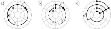
Figure 2: An ortho-radial drawing of a 4-cycle (a) and an ortho-radial representation of it that is not drawable (b), though the sum of the angles around each vertex and around each face is the same as in (a). A bend-optimal drawing of a graph (c), where the edge $e^{\prime}$ has bends in different directions.

Contribution and Outline.

We start with preliminary results in Section 2 introducing notions and facts on orthogonal and ortho-radial representations. In Section 3, we present an ILP for computing bend-free ortho-radial representations for graphs with a fixed embedding. In Section 4 we extend that ILP to optimize the number of bends. To that end, we provide theoretical insights into the number of bends required for ortho-radial drawings. Moreover, we describe a pruning strategy that allows us to quickly compute a bend-optimal drawing. In Section 5 we evaluate our algorithms and compare them to standard approaches for computing orthogonal drawings.

2 Preliminaries

A graph of maximum degree 4 is a 4-graph. Unless stated otherwise, all graphs occurring in this paper are 4-graphs. Let $G=(V,E)$ be a connected planar 4-graph with a fixed combinatorial embedding $\mathcal{E}$ and let $v\in V$ be a vertex. We call the counterclockwise order of edges around $v$ in the embedding the rotation of $v$, and we denote it by $\mathcal{E}(v)$. An angle at $v$ is a pair of edges $(e_{1},e_{2})$ that are both incident to $v$ and such that $e_{1}$ immediately precedes $e_{2}$ in $\mathcal{E}(v)$.

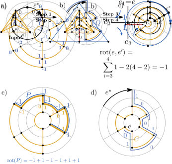
Figure 3: (a) Rotations between angles. (b) Rotations between two edges $e,e^{\prime}$. (c) Rotation of path $P$. (d) Label of edge $e$ with respect to essential cycle $C$.

Let $\Delta$ be an orthogonal (or ortho-radial) drawing of $G$ with embedding $\mathcal{E}$. By turning bends into vertices, we can assume that the drawing is bend-free. We now derive a labeling of the angles of $v$ with labels in $\{-2,-1,0,1\}$ with so-called rotation values. For an angle $(e_{1},e_{2})$ at $v$, we set $\operatorname{rot}(e_{1},e_{2})=2-2\alpha/\pi$, where $\alpha$ is the counterclockwise geometric angle between $e_{1}$ and $e_{2}$ in $\Delta$; see Fig. 3a. Intuitively, this counts the number of right turns one takes when traversing $e_{1}$ towards $v$ and afterwards $e_{2}$ away from $v$, where negative numbers correspond to left turns. Note that if $e_{1}=e_{2}$, then $\operatorname{rot}(e_{1},e_{2})=-2$, i.e., $v$ contributes two left turns.

For a face $f$ of $G$, we denote by $\operatorname{rot}(f)$ the sum of the rotations of all angles incident to $f$. Formally, if $v_{0},\dots,v_{n-1}$ is the facial walk around $f$ (oriented such that $f$ lies to the right of the facial walk), we define $\operatorname{rot}(f)=\sum_{i=0}^{n-1}\operatorname{rot}(v_{i-1}v_{i},v_{i}v_{i+1})$ where indices are taken modulo $n$. Intuitively, this counts the number of right turns minus the number of left turns one takes when traversing the face boundary such that the face $f$ lies to the right. Since $\Delta$ is an orthogonal drawing with some outer face $f_{o}$, it satisfies the following conditions [13].

1. For each vertex, the sum of the rotations around $v$ is $2(\deg(v)-2)$.

2. For each face $f\neq f_{0}$ it is $\operatorname{rot}(f)=4$ and it is $\operatorname{rot}(f_{0})=-4$.

We call an assignment $\Gamma$ of rotation values to the angles that satisfy these two rules an orthogonal representation. Every orthogonal drawing $\Delta$ induces an orthogonal representation. An orthogonal representation $\Gamma$ is drawable if there exits a drawing $\Delta$ that induces it.

For ortho-radial drawings a similar situation occurs. Here, we have two special faces; an unbounded face, called the outer face $f_{o}$, and a central face $f_{c}$, which contains the origin. If the central and the outer face are identical, then the drawing does not enclose the origin, and the ortho-radial drawing does in fact lie on some patch of the ortho-radial grid that can be conformally mapped to an orthogonal grid (i.e., without changing any angles). An ortho-radial drawing $\Delta$ similarly defines rotation values that satisfy the following conditions.

1. For each vertex, the sum of the rotations around $v$ is $2(\deg(v)-2)$.

2. For each face $f\neq f_{o},f_{c}$ it is $\operatorname{rot}(f)=4$, if $f_{o}\neq f_{c}$, then $\operatorname{rot}(f_{o})=\operatorname{rot}(f_{c})=0$ and $\operatorname{rot}(f_{o})=-4$ if $f_{o}=f_{c}$.

Similar to the orthogonal case, an ortho-radial drawing $\Delta$ therefore induces an ortho-radial representation $\Gamma$ that defines rotation values satisfying these conditions. An ortho-radial representation is drawable if there exists an ortho-radial drawing that induces it.

Tamassia [13] proved that every orthogonal representation is drawable. In contrast, there exist ortho-radial representations that are not drawable; see e.g., Fig. 2b, which illustrates a so-called strictly monotone cycle. Its ortho-radial representation satisfies conditions (I)’ and (II)’, yet it is not drawable.

To characterize the drawable ortho-radial representations, Barth et al. [1] introduce a labeling concept. Since the horizontal and vertical directions on an ortho-radial grid are not interchangeable (one is circular, the other is not), additional information is required. The information which is the horizontal direction is given by a reference edge ${e^{\star}}$ which is assumed to lie on the outer face and that is directed such that it points in the clockwise direction. To present the characterization of Barth et al. [1], we extend the notion of rotation. For two edges $e,e^{\prime}$ incident to a vertex $v$, let $e=e_{1},\dots,e_{k}=e^{\prime}$ be the edges between them in $\mathcal{E}(v)$ so that $(e_{i},e_{i+1})$ is an angle for $i=1,\dots,k-1$. To measure the rotation between $e$ and $e^{\prime}$, we convert the rotation values between them into geometric angles, sum them up, and convert them back to a rotation, which gives $\operatorname{rot}(e,e^{\prime})=\sum_{i=1}^{k-1}\operatorname{rot}(e_{i},e_{i+1})-2(k-2)$; see Fig. 3b. Note that for an angle $(e,e^{\prime})$, it is $k=2$, and therefore the two definitions of $\operatorname{rot}(e,e^{\prime})$ coincide. For a path $P=v_{0},\dots,v_{n-1}$ in $G$, we define its rotation $\operatorname{rot}(P)=\sum_{i=1}^{n-1}\operatorname{rot}(v_{i-1}v_{i},v_{i}v_{i+1})$, and for a cycle $C$ in $G$, we define its rotation $\operatorname{rot}(C)=\sum_{i=1}^{n}\operatorname{rot}(v_{i-1}v_{i},v_{i}v_{i+1})$, where indices are taken modulo $n$; see Fig. 3c. A cycle $C$ of $G$ is called essential if it separates the central and the outer face. A cycle is essential if and only if $\operatorname{rot}(C)=0$ [1]. We assume that $C$ is directed such that the central face lies to its right. Let $e$ be an edge on $C$. A reference path for $e$ on $C$ is a (not necessarily simple) walk $P$ that starts with the edge ${e^{\star}}$, ends with the edge $e$ and does not contain an edge or a vertex that lies to the right of $C$. We define $\ell_{C}(e)=\operatorname{rot}(P)$ as the label of $e$ on $C$; see Fig. 3d. Barth et al. [1] show that the label does not depend on the actual path $P$ (however the same edge may have different labels for different cycles). With this, Barth et al. formulate a third condition. An ortho-radial representation is called valid if, for each essential cycle $C$, either $\ell_{C}(e)=0$ for all edges $e\in E(C)$, or there exist edges $e^{-},e^{+}$ in $E(C)$ with $\ell_{C}(e^{-})<0$ and $\ell_{C}(e^{+})>0$. A cycle $C$ that does not satisfy this condition is called strictly monotone. Thus, an ortho-radial representation is valid if and only if it has no strictly monotone cycle. In Fig. 2a,b the edges of the 4-cycle are labeled with their labels with respect to the reference edge ${e^{\star}}$; Fig. 2b is a strictly monotone cycle. The following two results form the combinatorial and algorithmic basis for our work.

Theorem 2.1 (Barth et al. [1])

An ortho-radial representation is drawable if and only if it is valid.

Theorem 2.2 (Niedermann et al. [12])

There is an $O(n^{2})$-time algorithm that, given an ortho-radial representation $\Gamma$ of an $n$-vertex graph $G$, either outputs a drawing of $\Gamma$, or a strictly monotone cycle $C$ in $\Gamma$.

3 ILP for Bend-Free Ortho-Radial Drawings

In this section we are given a planar 4-graph $G=(V,E)$ with a combinatorial embedding $\mathcal{E}$, an outer face $f_{o}$, a central face $f_{c}$ and a reference edge ${e^{\star}}$ on $f_{o}$; we denote that instance by $\mathcal{G}=(G,\mathcal{E},f_{o},f_{c},{e^{\star}})$. We present an algorithm based on an ILP that yields a valid ortho-radial representation of $\mathcal{G}$, if it exists.

Basic Formulation.

For each vertex $u$ and each of its angles $(e,e^{\prime})$ we introduce an integer variable $r_{e,e^{\prime}}\in\{-2,-1,0,1\}$, which describes the rotation $\operatorname{rot}(e,e^{\prime})$ between $e$ and $e^{\prime}$. Condition I’ is enforced by the following constraint for $u$.

$$\sum^{k}_{i=1}r_{e_{i},e_{i+1}}=2(\deg(v)-2),$$ (1)

where $e_{1},\dots,e_{k}$ are the incident edges of $u$ in counter-clockwise order; we define $e_{k+1}=e_{1}$. For each face $f$ of $\mathcal{G}$ Condition II’ is enforced by the next constraint.

$$\sum_{i=1}^{k}r_{e_{i},e_{i+1}}=\begin{cases}4&\text{if $f$ is a regular face,}\\ 0&\text{if $f$ is the outer or central face but not both,}\\ -4&\text{if $f$ is both the central and outer face,}\end{cases}$$ (2)

where $e_{1},\dots,e_{k}$ are the edges of the facial walk around $f$ such that $f$ lies to the right; we define $e_{k+1}=e_{1}$. We denote that formulation by $\mathcal{F}_{\mathrm{or}}$. By construction a valid assignment of the variables in $\mathcal{F}_{\mathrm{or}}$ induces an ortho-radial representation $\Gamma$. In particular, assuming that $e^{\star}$ is directed such that it points clockwise, we can derive from the variable assignment the directions of the other edges in $G$. The next theorem summarizes this result.

Theorem 3.1

An ortho-radial representation exists for $\mathcal{G}$ if and only if $\mathcal{F}_{\mathrm{or}}$ induces an ortho-radial representation.

Figure 4: Illustration of path Q used for the labeling of $C$.

However, the induced ortho-radial representation $\Gamma$ is not necessarily valid, but may contain strictly monotone cycles. We therefore extend $\mathcal{F}_{\mathrm{or}}$ by constraints for each essential cycle $C$ of $\mathcal{G}$. To that end, let $P$ be a path that starts at ${e^{\star}}$ and ends at $C$ such that it does not use any vertex or edge that lies to the right of $C$. Further, let $Q$ be the path ${e^{\star}}+P+C$ that follows $C$ in clockwise order from the endpoint of $P$ and ends at the end point of $P$; see Fig. 4. For each edge $e$ of $Q$ we introduce an integer variable $l_{e}$ with $-m\leq l_{e}\leq m$, which models a label with respect to $C$. Here $m$ denotes the number of edges of $G$. We require that the label of the reference edge is $0$, i.e., $l_{e^{\star}}=0$. Moreover, for an edge $e=vw$ of $Q\setminus\{e^{\star}\}$ and its predecessor $e^{\prime}=uv$ on $Q$ let $e^{\prime}=e_{1},\dots,e_{k}=e$ be the edges between them in $\mathcal{E}(v)$ so that $(e_{i},e_{i+1})$ is an angle for $i=1,\dots,k-1$. We introduce the constraint

$$l_{e}=l_{e^{\prime}}+\sum_{i=1}^{k-1}r_{e_{i},e_{i+1}}-2(k-2)$$ (3)

Hence, the values $l_{e}$ for $e\in E(C)$ describe a labeling of $C$, where $E(C)$ denotes the edges of $C$. To exclude strictly monotone cycles, we ensure that either $l_{e}=0$ for all edges $e\in E(C)$, or there exist edges $e^{-},e^{+}$ in $E(C)$ with $l_{e^{-}}>0$ and $l_{e^{+}}<0$. We first observe that $C$ can only be strictly monotone if $\sum_{e\in E(C)}l_{e}\neq 0$. We introduce a single binary variable $z$ that is $1$ if and only if $\sum_{e\in E(C)}l_{e}=0$. Additionally, for each edge $e$ of $C$ we introduce two binary variables $x_{e}$ and $y_{e}$, which are used to enforce that $l_{e}$ is negative or positive, respectively.

$$\sum_{e\in E(C)}l_{e}\leq M\cdot(1-z)$$ (4)

$$\sum_{e\in E(C)}l_{e}\geq-M\cdot(1-z)$$ (5)

$$\sum_{e\in E(C)}x_{e}+z\geq 1$$ (6)

$$\sum_{e\in E(C)}y_{e}+z\geq 1$$ (7)

$$l_{e}\leq-1+M\cdot(1-x_{e})\ \forall e\in E(C)$$ (8)

$$l_{e}\geq 1-M\cdot(1-y_{e})\ \forall e\in E(C)$$ (9)

We define $M$ as a constant with $M>m$ so that the corresponding constraints are trivially satisfied for $z=0$, $x_{e}=0$ and $y_{e}=0$, respectively. If $z=1$, we obtain by Constraint 4 and Constraint 5 that $\sum_{e\in E(C)}l_{e}=0$. Hence, $C$ is not strictly monotone. Otherwise, if $z=0$, by Constraint 6 there is an edge $e^{-}\in E(C)$ with $x_{e^{-}}=1$. By Constraint 8 we obtain $l_{e^{-}}<0$. Similarly, by Constraint 7 there is an edge $e^{+}\in E(C)$ with $y_{e^{+}}=1$. By Constraint 9 we obtain $l_{e^{+}}>0$. Altogether, we find that $C$ is not strictly monotone. We emphasize that for each essential cycle $C$ of $\mathcal{G}$ we introduce a fresh set of variables and constraints; which we denote by $\mathcal{F}_{C}$. Hence, we consider the ILP $\mathcal{F}(\mathcal{G})=\mathcal{F}_{\mathrm{or}}\cup\bigcup_{C\in\mathcal{C}}\mathcal{F}_{C}$, where $\mathcal{C}$ is the set of all essential cycles in $\mathcal{G}$. The next theorem summarizes this.

Theorem 3.2

If $\mathcal{G}$ has an ortho-radial representation, then the formulation $\mathcal{F}(\mathcal{G})$ induces a valid ortho-radial representation.

Separation of Constraints.

Adding $\mathcal{\mathcal{missing}}F_{C}$ for each essential cycle $C$ of $\mathcal{G}$ is not feasible in practice, as there can be exponentially many of these in $\mathcal{G}$. Hence, instead, we propose an algorithm that adds $\mathcal{F}_{C}$ on demand. The algorithm first checks whether $\mathcal{G}$ has an ortho-radial representation $\Gamma_{1}$ using the formulation $\mathcal{F}_{1}:=\mathcal{F}_{or}$ (Theorem 3.1). If this is not the case, the algorithm stops and returns that there is no ortho-radial representation for $\mathcal{G}$. Otherwise, starting with $\mathcal{F}_{1}$ and $\Gamma_{1}$ it applies the following iterative procedure. In the $i$-th iteration (with $2\leq i$) it checks whether $\Gamma_{i-1}$ is valid (Theorem 2.2). If it is, the algorithm stops and returns $\Gamma_{i-1}$. Otherwise, the validity test yields a strictly monotone cycle $C$ as a certificate proving that $\Gamma_{i-1}$ is not valid. The algorithm creates then the formulation $\mathcal{F}_{i}=\mathcal{F}_{i-1}\cup\mathcal{F}_{C}$ and induces the ortho-radial representation $\Gamma_{i}$, in which it is enforced that $C$ is not strictly monotone. The algorithm stops at the latest when the formulation $\mathcal{F}_{C}$, which prohibits that $C$ is a strictly monotone cycle, has been added for each essential cycle $C\in\mathcal{C}$. Hence, in theory an exponential number of iterations may be necessary. However, in our experiments the procedure stopped after few iterations for all test instances; see Section 5.

Bend Optimization.

We also can use the ILP to optimize the ortho-radial representation. In Section 4 we consider bend minimization by modeling bends as degree-2 vertices. We therefore extend $\mathcal{F}_{\mathrm{or}}$ such that it allows us to optimize the change of direction at such nodes. For each degree-2 vertex we introduce a binary variable $c_{u}$, which is $1$ if and only if one of the two incident edges of $u$ lies on a concentric circle and the other lies on a ray of the grid. The two incident edges $e_{1}$ and $e_{2}$ of $u$ form the two angles $(e_{1},e_{2})$ and $(e_{2},e_{1})$. For these we introduce the constraints $c_{u}\geq r_{e_{1},e_{2}}$ and $c_{u}\geq r_{e_{2},e_{1}}$. Subject to these constraints we minimize $\sum_{u\in V_{2}}c_{u}$, where $V_{2}\subseteq V$ denotes the degree-2 vertices of $G$. We can easily restrict the optimization to a subset of $V_{2}$ distinguishing between degree-2 vertices that originally belong to $G$ and those that we use for modeling bends.

4 Optimizing Bends and the Choice of the Central Face

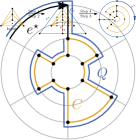
Figure 5: Illustration of the layout algorithm. Subdivision vertices are squares.

In this section we are given a graph $G$ with embedding $\mathcal{E}$ and designated outer face $f_{o}$. We describe an algorithm that returns a bend-optimal ortho-radial drawing for $\mathcal{G}=(G,\mathcal{E},f_{o})$, i.e., there is no other ortho-radial drawing $\mathcal{G}$ that has fewer bends for any choice of the central face $f_{c}$ and the reference edge $e^{\star}$ on $f_{o}$. The algorithm uses the ILP from Section 3 as a building block. The ILP does not directly allow to express bends; rather, we subdivide the edges with degree-2 vertices, which can then be used as bends. See Fig. 5 for an illustration.

1. Insert a cycle $C_{o}$ in $\mathcal{E}$ that encloses $G$ and connect $C_{o}$ via an edge $\epsilon$ to a newly inserted vertex $\nu$ on the original outer face of $\mathcal{E}$. Insert edge $\epsilon^{\prime}$ on the opposite side enforcing that $\nu$ has degree 4. Hence, $C_{o}$ is the new boundary of the outer face $f_{o}$. Choose an arbitrary edge of $C_{o}$ as reference edge $e^{\star}$.

2. Subdivide each edge of $G$ with degree-2 vertices such that each maximally long chain of degree-2 vertices consists of at least $K$ vertices.

3. Create a valid ortho-radial representation $\Gamma_{f}$ for face $f$ as the central face. To that end, apply the ILP formulation of Section 3 with separated constraints and bend optimization on $\mathcal{G}_{f}=(G,\mathcal{E},f_{o},f,e^{\star})$ charging the newly inserted degree-2 vertices with costs; the subdivision vertices on $\epsilon$ are not charged.

4. For the representation $\Gamma_{f}$ with fewest bends compute a drawing (Theorem 2.2).

Figure 6: Constructions for the proof of Theorem 4.1

For bend-optimal drawings an appropriately large $K$ is decisive. For biconnected graphs $K=2n+4$ is sufficient even for a fixed central and outer face.

Theorem 4.1

Every biconnected plane 4-graph on $n$ vertices with designated central and outer faces has a planar ortho-radial drawing with at most $2n+4$ bends and at most two bends per edge with the exception of up to two edges that may have three bends.

The proof, which is deferred to Appendix 0.A, uses similar constructions as in the orthogonal case; see also Fig. 6. It seems plausible that the bound can be transferred to non-biconnected graphs as in the work by Biedl and Kant [3]; as we use a different bound, we refrain from the rather technical proof. Moreover, we insert $C_{o}$ to make the layout independent from the choice of the reference edge ${e^{\star}}$. This does not impact the number of bends needed for the original part of $G$, because we subdivide $\epsilon$ with sufficiently many 2-degree vertices that can be bent for free. Further, as $\nu$ has degree 4, the drawing cannot be bent at $\nu$.

Replacing each edge by $2n+4$ degree-2 vertices increases the size of the graph drastically. However, the ILP can be solved much faster if fewer subdivision vertices are used. Next, we describe a pruning strategy that uses upper and lower bounds on the optimal drawing to exclude central faces and to limit the number of subdivision vertices and the number of times we solve the ILP.

We first compute the minimum number $U$ of bends that is necessary for a bend-optimal orthogonal drawing of $\mathcal{G}$. This also bounds the number of bends in a bend-optimal ortho-radial drawing of $\mathcal{G}$. Hence, it is sufficient to subdivide each edge with $U$ vertices in Step 2. Initially, we run $\mathcal{F}_{\mathrm{or}}$ on each face $f$ of $\mathcal{G}$ as central face. This gives us a lower bound $l_{f}$ for the bends in the case that $f$ is the central face. In Step 3 we then consider the faces in increasing order of their lower bounds. If the lower bound $l_{f}$ of the current face $f$ exceeds the upper bound $U$ we prune $f$ and continue with the next face. Otherwise, we iteratively compute a valid ortho-radial representation $\Gamma_{f}$ for $f$ as described in Section 3 and update $U$ if it is improved by the current solution. Further, when we update the ILP due to strictly monotone cycles, we skip $f$ if its number of bends exceeds $U$ and continue with the next face.

5 Experimental Evaluation

In this section we present our experimental evaluation which we have conducted to show the potential of our approach as a general graph drawing tool.

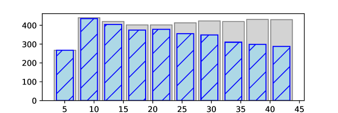
Figure 7: The node distribution (gray bars) of the graphs in $\mathcal{I}_{\text{Rome}}$ distributed on 10 equally sized bins. The number of vertices ranges between 3 and 44. The blue, tiled bars indicate the number of optimally solved instances.

5.1 Feasibility of Approach

We first pursue the issue of whether our approach is feasible. It is far from clear whether prohibiting strictly monotone cycles on demand is practical, as we may need to insert an exponential number of constraints into the ILP formulation. To answer this question we have conducted the first experiments on a subset of the Rome graphs, which is a widely accepted benchmark set. We have replaced each vertex $v$ with degree $k>4$ with a cycle of $k$ vertices, which we connected to the neighbors of $v$ correspondingly. Further, we applied a heuristic from OGDF [6] to embed the remaining graphs such that the size of the outer face is maximized. We replaced all edge crossings with degree-4 vertices. A preliminary analysis showed that the graphs contain many degree-2 vertices. To ensure for the purpose of the evaluation that our approach is forced to introduce bends with costs, we normalized each instance by removing all degree-2 vertices. We only considered instances up to 44 nodes. In total we obtained a set $\mathcal{I}_{\text{Rome}}$ of $4048$ instances. Figure 7 shows the size distribution of the resulting instances. We implemented our approaches in Python and solved the ILP formulations using Gurobi 9.0.2 [9] using a timeout of 2 minutes in each iteration. We ran the experiments on an Intel(R) Xeon(R) W-2125 CPU clocked at 4.00GHz with 128 GiB RAM.

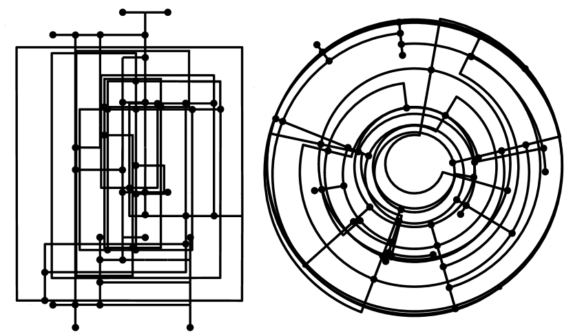
Figure 8: Examples of bend-optimal orthogonal and ortho-radial drawings for the Rome graphs. The outer face was fixed, but the central face was optimized.

For each of the instances in $\mathcal{I}_{\text{Rome}}$ we applied the algorithm described in Section 4; see Fig. 8 for four examples. For $3462$ instances we obtained bend-optimal ortho-radial drawings. For $586$ instances the solver returned a not necessarily optimal result due to timeouts. The number of not optimally solved instances increases with the number of nodes; see Fig. 7 for more details. For $1081$ instances the algorithm took less than half a second. Only for $861$ instance it took more than 10 seconds; $628$ of them took more than one minute. Further, when searching for the best choice of the central face about 76.5$\%$ of the faces are pruned in advance on average due to exceeding upper bounds. Hence, for more than three quarters of the faces we do not need to solve the ILP formulation, still guaranteeing that we obtain a drawing with minimum number of bends. Moreover, when the algorithm runs for a fixed central face, it needs less than $3.8$ iterations on average until it finds a valid ortho-radial representation. Put differently, we insert the formulation $\mathcal{F}_{C}$ prohibiting a strictly monotone cycle $C$ into the ILP formulation $3.8$ times on average. Altogether, the evaluation shows the practical feasibility of the approach. It supports the rather strong hypothesis that prohibiting strictly monotone cycles on demand is sufficient, but considering all essential cycles is not necessary.

Figure 9: Overview of the considered Rome graphs. A disk with radius $r$ and position $(x,y)$ corresponds to $r$ instances (a) with $x$ vertices and $y$ bends in the ortho-radial (blue) and the orthogonal (red) drawing, (b) with $x$ bends in the orthogonal drawing and $y$ bends in the ortho-radial drawing.

5.2 Ortho-radial Drawings vs. Orthogonal Drawings

In this part we compare ortho-radial drawings with orthogonal drawings with respect to the necessary number of bends. We expect a reduction of the number of bends in an ortho-radial drawing compared with its orthogonal drawing.

Fig. 9a shows that independent of the size of the graphs the ortho-radial drawings often have fewer bends than the orthogonal drawings. Further, Fig. 9b shows that for many of the instances we achieve a reduction between 1 to 3 bends in the ortho-radial drawings. To investigate this in greater detail we consider for each instance $I\in\mathcal{I}_{\text{Rome}}$ the bend reduction $r_{I}=\frac{b_{\mathrm{og}}-b_{\mathrm{or}}}{b_{\mathrm{og}}}\cdot 100\%$, where $b_{\mathrm{og}}$ is the minimum number of bends of an orthogonal drawing of $I$ and $b_{\mathrm{or}}$ is the number of bends of the ortho-radial drawing created with our approach; note that for both drawings we assume the same embedding and the same outer face. From this comparison we have excluded any instance with zero bends. The bend reduction is 43.8$\%$ on average and the median is at 40.0$\%$. We emphasize that for $550$ instances there are bend-free ortho-radial drawings, whereas only $129$ admit bend-free orthogonal drawings. Thus, our experiments support our hypothesis that ortho-radial drawings lead to a substantial bend reduction.

(a)

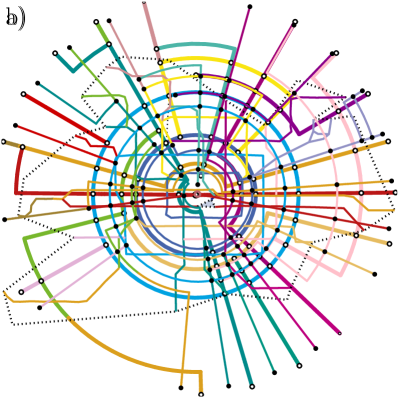
(b)

Figure 10: The metro system in Beijing, China. (a) The input graph derived from vectorizing a metro map of Beijing. The outer and central faces are dashed. (b) The ortho-radial layout induced by our approach within 7 seconds.

5.3 Case Study on Metro Maps

Ortho-radial drawings are particularly used to represent metro systems [14]. We tested our algorithm on the metro system of Beijing, which is a comparably large and complex transit system; see Fig 10. We have vectorized a metro map of the city that shows 21 lines; for details see Appendix 0.B.1. The created graph has 224 vertices, 289 edges and 67 faces. We fixed the central face by hand to intentionally determine the appearance of the final layout. We subdivided the edges such that each chain consisting of degree-2 vertices has at least three intermediate vertices. Our algorithm created the layout shown in Fig. 10b within seven seconds. It has 21 bends. We emphasize that the outer loop line is represented as a circle and the inner loop line has only two bends. Altogether, the layout reflects the main geometric features of the system well, although we have only optimized the number of bends, e.g., outgoing metro lines are mainly drawn as straight-lines emanating from the center. In a second run, which took three minutes, we proved that 21 bends is optimal. Further metro systems are found in Appendix 0.B.2.

6 Conclusion

Barth et al. [1] and Niedermann et al. [12] carried over the metrics step of the TSM framework from orthogonal to ortho-radial drawings explaining how to obtain such a drawing from a valid ortho-radial representation. However, they let open how to transfer the shape step constructing such a valid ortho-radial representation. We presented the first algorithm that answers this question and creates ortho-radial drawings, which are bend-optimal. Our experiments showed its feasibility based on the Rome graphs and different metro systems. This was far from clear due to the possibly exponential number of essential cycles.

Altogether, we presented a general tool for creating ortho-radial drawings. We see applications in map making (e.g., metro maps, destinations maps). Possible future refinements include the adaption of the optimization criteria both in the shape and metrics step. For example in the shape step one could enforce certain bends to better express the geographic structure of the transit system.

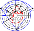
Figure 11: Example of the algorithm from Theorem 4.1 applied to the octahedron graph. The central face is marked with a cross, the numbers indicate the st-ordering that was used.

Appendix 0.A Omitted Proof of Section 4

Theorem 0.A.1

Every biconnected plane 4-graph on $n$ vertices with designated central and outer faces has a planar ortho-radial drawing with at most $2n+4$ bends and at most two bends per edge with the exception of up to two edges that may have three bends.

Proof

Let $G$ be a biconnected 4-plane graph and let $s,t$ be two vertices incident to the central and outer face, respectively, that are not adjacent. Let $\langle s=v_{1},\dots,v_{n}=t\rangle$ be an st-ordering of $G$.

Figure 12: Illustration of the incremental drawing step. Drawing of the first vertex $v_{1}$, depending on its degree (a); the edges incident to the central face are thick and red. Drawing of the intermediate vertices depending on their in- and outdegrees (b,c). Drawing of the last vertex $v_{n}$ depending on its degree (d); the edges incident to the outer face are thick and blue.

Our construction iteratively places each vertex $v_{i}$ onto the circle with radius $i$ around the origin; the construction is illustrated in Figure 11. Edges where both endpoints have already been placed are drawn, edges where exactly one endpoint has already been placed, are partial. Note that, when inserting an edge, at least one partial edge becomes drawn, and at most three edges become partial.

Throughout, we maintain the invariant that (i) all drawn edges (except at most one incident to $v_{1}$ and $v_{n}$, each) have at most two bends , (ii) they are contained in the disk with radius $i$, and (iii) the half-edges are drawn as stubs with at most one bend such that (iv) only an outward-directed segment lies outside the disk with radius $i$, and these end at the circle with radius $i+0.5$. Moreover, since we have an $st$-ordering, for each $i<n$ the vertices $v_{1},\dots,v_{i}$ and the vertices $v_{i+1},\dots,v_{n}$ induce connected subgraphs. Therefore the cut $C$ separating them is represented by a simple curve in the dual. We further require (v) that our drawing respects the planar embedding in the sense that the circular order of the stubs around this circle is the same as the order in which the they are intersected by the cycle that is dual to $C$.

Depending on the degree of $v_{1}$, we draw it together with its half-edges as illustrated in Fig. 12a; where we choose the directions in which the edges leave $v$ so that the edges incident to the central face are drawn as indicated by the thick blue curves. This clearly establishes properties (i)–(v). Suppose $1<i<n$. Let $u_{1},\dots,u_{k}$ with $1\leq k\leq 4$ be the neighbors of $v_{i}$ that are already drawn. By property (v) and the fact that we have an st-ordering, it follows that the ends of the half-edges from the $u_{j}$ to $v_{i}$ are consecutive around the circle with radius $i-0.5$. Depending on the in- and out-degree, we position $v$ in the outward direction above one of its incoming edges and draw the outgoing edges as illustrated in Fig. 12b,c, where the spokes that contain the outgoing edges of $v$ are newly created left and right of the spoke that contain $v_{i}$, and the remaining spokes are slightly squeezed to make sufficient space. All remaining stubs are simply extended by one unit in the outward direction. Finally, we palce the vertex $v_{n}$ as illustrated in Fig. 12d; making sure that it is positioned in the outward direction above one of its incoming edges in such a way that the correct faces lies on the outside.

Clearly each edge, except for one edge incident to $v_{1}$ and $v_{4}$ receive at most two bends (one when its first vertex is drawn, and one when the second vertex is drawn. Moreover, each vertex causes bends on at most two of its incident vertices, which yields an upper bound of at most $2n$ bends. Moreover, the special edges incident to $v_{1}$ and $v_{n}$ receive two additional bends, which yields the claimed total of $2n+4$.

Appendix 0.B Metro Maps

0.B.1 Vectorization of the Metro System of Beijing

We vectorized the metro system of Beijing as follows. We connected crossings between metro lines and terminal stations by paths consisting of degree-2 vertices. We refrained from modeling the intermediate stations as degree-2 vertices; one may distribute them on the sections of the metro lines after creating the ortho-radial layout. The metro system has only one degree-5 vertex. We resolved this vertex by reconnecting one of the five edges to one additional vertex subdividing a neighboring edge. Further, we have replaced the station Tiananmen East, which lies in the center of the city, by a cycle of three edges. We have fixed this cycle as the boundary of the central face. Further, we have connected the terminal stations of the outgoing lines by a cycle enclosing the entire system; we fixed this cycle as the boundary of the outer face. The resulting graph has 224 vertices, 289 edges and 67 faces.

0.B.2 Additional Examples

In Figure 14 and Figure 14 we present ortho-radial layouts for the metro systems of Cologne, Germany and London, UK. We extracted the graphs to obtain large examples for our feasibility study. In particular, we do not claim that the layouts correctly represent the transit systems. Especially for the London metro system we resolved several degree-5 vertices modeling them as cycles. Hence, as we do not impose any restrictions on the layout, geographically close stations may be placed far away from each other in the layout. We deem the task of transferring the algorithm to produce reliable metro maps to be an engineering problem that should be tackled in future work.

(a)

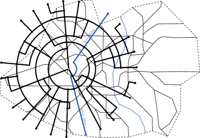
(b)

Figure 13: The metro system of Cologne, Germany. The river Rhine, which passes through the city, is marked blue. (a) The input graph derived from vectorizing the official metro map of Cologne. We replaced the station Heumarkt, which lies in the center of the city, with a cycle and fixed this as the central face. The outer and central faces are dashed. The graph has 177 vertices, 231 edges and 56 faces. (b) The ortho-radial layout produced by our approach within 2 seconds. It has 18 bends.

(a)

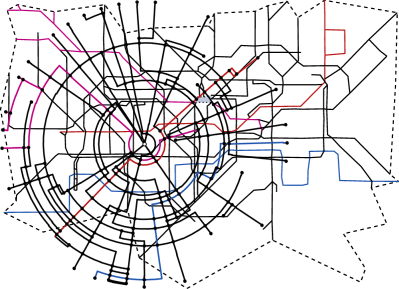
(b)

Figure 14: The metro system of London, UK. We have marked two lines by their color and the river Thames (blue) to give orientations. (a) The input graph derived from vectorizing the official metro map of London. We modeled the area around King’s Cross with a cycle and fixed this as the central face. The outer and central faces are dashed. The graph has 398 vertices, 530 edges and 134 faces. (b) The ortho-radial layout produced by our approach within 9 seconds. It has 62 bends.

References

- [1] Barth, L., Niedermann, B., Rutter, I., Wolf, M.: Towards a topology-shape-metrics framework for ortho-radial drawings. In: Aronov, B., Katz, M.J. (eds.) Computational Geometry (SoCG’17). Leibniz International Proceedings in Informatics (LIPIcs), vol. 77, pp. 14:1–14:16. Schloss Dagstuhl–Leibniz-Zentrum fuer Informatik (2017)
- [2] Biedl, T., Kant, G.: A better heuristic for orthogonal graph drawings. In: van Leeuwen, J. (ed.) Algorithms (ESA’94). LNCS, vol. 855, pp. 24–35. Springer (1994)
- [3] Biedl, T., Kant, G.: A better heuristic for orthogonal graph drawings. Computational Geometry 9(3), 159 – 180 (1998)
- [4] Bläsius, T., Rutter, I., Wagner, D.: Optimal orthogonal graph drawing with convex bend costs. ACM Transactions on Algorithms 12(3), 33 (2016)
- [5] Bläsius, T., Lehmann, S., Rutter, I.: Orthogonal graph drawing with inflexible edges. Computational Geometry 55, 26 – 40 (2016)
- [6] Chimani, M., Gutwenger, C., Jünger, M., Klau, G.W., Klein, K., Mutzel, P.: The Open Graph Drawing Framework (OGDF). In: Tamassia, R. (ed.) Handbook of Graph Drawing and Visualization, chap. 17, pp. 543–569. CRC Press (2013)
- [7] Duncan, C.A., Goodrich, M.T.: Handbook of Graph Drawing and Visualization, chap. Planar Orthogonal and Polyline Drawing Algorithms, pp. 223–246. CRC Press (2013)
- [8] Felsner, S., Kaufmann, M., Valtr, P.: Bend-optimal orthogonal graph drawing in the general position model. Computational Geometry 47(3, Part B), 460–468 (2014), special Issue on the 28th European Workshop on Computational Geometry (EuroCG 2012)
- [9] Gurobi Optimization, L.: Gurobi optimizer reference manual (2020), http://www.gurobi.com
- [10] Hasheminezhad, M., Hashemi, S.M., McKay, B.D., Tahmasbi, M.: Rectangular-radial drawings of cubic plane graphs. Computational Geometry: Theory and Applications 43, 767–780 (2010)
- [11] Hasheminezhad, M., Hashemi, S.M., Tahmasbi, M.: Ortho-radial drawings of graphs. Australasian Journal of Combinatorics 44, 171–182 (2009)
- [12] Niedermann, B., Rutter, I., Wolf, M.: Efficient algorithms for ortho-radial graph drawing. In: Barequet, G., Wang, Y. (eds.) Proceedings of the 35th International Symposium on Computational Geometry (SoCG’19). Leibniz International Proceedings in Informatics (LIPIcs), vol. 129, pp. 53:1–53:14. Schloss Dagstuhl–Leibniz-Zentrum fuer Informatik (2019)
- [13] Tamassia, R.: On embedding a graph in the grid with the minimum number of bends. Journal on Computing 16(3), 421–444 (1987)
- [14] Wu, H.Y., Niedermann, B., Takahashi, S., Roberts, M.J., Nöllenburg, M.: A survey on transit map layout – from design, machine, and human perspectives. Computer Graphics Forum 39(3) (2020)