A Strategic Routing Framework and
Algorithms for Computing Alternative Paths

Abstract

Traditional navigation services find the fastest route for a single driver. Though always using the fastest route seems desirable for every individual, selfish behavior can have undesirable effects such as higher energy consumption and avoidable congestion, even leading to higher overall and individual travel times. In contrast, strategic routing aims at optimizing the traffic for all agents regarding a global optimization goal. We introduce a framework to formalize real-world strategic routing scenarios as algorithmic problems and study one of them, which we call Single Alternative Path (SAP), in detail. There, we are given an original route between a single origin–destination pair. The goal is to suggest an alternative route to all agents that optimizes the overall travel time under the assumption that the agents distribute among both routes according to a psychological model, for which we introduce the concept of Pareto-conformity. We show that the SAP problem is NP-complete, even for such models. Nonetheless, assuming Pareto-conformity, we give multiple algorithms for different variants of SAP, using multi-criteria shortest path algorithms as subroutines. Moreover, we prove that several natural models are in fact Pareto-conform. The implementation of our algorithms serves as a proof of concept, showing that SAP can be solved in reasonable time even though the algorithms have exponential running time in the worst case.

1 Introduction

Commuting is part of our daily lives. Street congestion, traffic jams and pollution became an increasingly large issue in the last few decades. In German cities, these effects caused costs of about 3 billion euros in 2019 [11]. Many traffic jams in cities could have been avoided by better route choice. Partly this is because of non-optimal route choices by individuals due to bounded rationality and route preferences other than “fastest” [30]. However, even with individually optimal route choice, average travel time can be substantially worse compared to a system optimum where all routes are centrally assigned [22]. Thus, there is an opportunity for improving traffic via strategic routing where (re)routing recommendations are created by traffic authorities and taken into account by the driver’s routing system. More precisely, we speak of strategic routing when two conditions are met:

1. One or more routes are calculated to be proposed to more than one agent, and

2. the quality of a set of proposed routes is being defined by a shared scoring rather than scoring each agent individually.

Recent research indicates that many drivers would accept individually slower routes if this contributes to an overall reduction in traffic [27, 14]; additionally, incentives such as free parking could be granted to those accepting these routes, and future autonomous vehicles may be more amenable to centralized control. Thus, (re)routing recommendations can have a strong impact since they might be followed by a significant fraction of all drivers.

In the ongoing pilot research project Socrates 2.0, strategic routing is employed in the area of Amsterdam [25]. For this, experts predefine alternative routes and traffic conditions that trigger their recommendation. This requires extensive work and monitoring, and does not capture well unusual traffic situations where there might be several incidents at once causing delays. Thus, it is desirable to automate this by formalizing strategic routing and finding algorithms that calculate strategic routes.

Our Contribution.

Strategic routing as defined above is not a single algorithmic problem but rather a concept capturing numerous scenarios leading to different problems. In Section 2, we provide a framework to guide the process of formalizing real-world strategic routing scenarios. We apply it to one specific scenario, namely Single Alternative Path (SAP). This scenario is inspired by the Amsterdam use case mentioned above where congestion can be prevented by suggesting one alternative route to all agents, e.g., via a variable-message sign. We consider different psychological models to determine how many agents follow the suggestion. Moreover, we consider variants of the SAP problem that require the alternative to be more or less disjoint from the original route. See Section 2.2 for a formal definition.

To tackle SAP algorithmically, we introduce the concept of Pareto-conformity of psychological models and, based on this, give various algorithms in Section 3. As they use multi-criteria shortest path algorithms as subroutine, they have an exponential worst-case running time but turn out to be sufficiently efficient in practice; see our evaluation in Section 6. Moreover, in this generality, we cannot hope for better worst-case bounds as SAP is NP-hard, even for Pareto-conform psychological models; see Section 5. In Section 4, we prove the Pareto-conformity of three natural psychological models. Our proofs actually hold for the more general and abstract Quotient Model that captures various additional models. We evaluate our algorithms in Section 6. It serves as a proof of concept that our algorithms have reasonable practical run times and yield promising travel time improvements for instances in the traffic network of Berlin.

Related Work.

There has been no unique understanding of strategic routing in research until this point. Van Essen [27] uses a choice-theoretical approach and concludes that individual route choice and travel information that stimulates non-selfish user behavior have a large impact on the network efficiency. Kröller et al. [14] investigate due to what kind of incentives agents would deviate from the shortest-path route. Their results show that certain incentives can increase the drivers’ willingness of taking detours. Moreover, they show that there is a high interest in services providing alternative routes, and strategic routing is considered to have the potential of solving traffic issues such as congestion and pollution.

For standard algorithmic techniques in efficient route planning, we refer to the survey of Bast et al. [2]. Köhler et al. [15] deal with finding static and also time-dependent traffic flows minimizing the overall travel time. Also, as stated by Strasser [26], routing with predicted congestion is well-studied, e.g., by Delling and Wagner [7], Demiryurek et al. [8], Delling [5] and Nannicini et al. [19]. Route planning with alternative routes was investigated by Abraham et al. [1] and Paraskevopoulos and Zaroliagis [21]. They propose algorithms that find alternative routes by evaluating properties with regard to an original route.

Lastly, we emphasize that strategic routing is very different from selfish routing as proposed by Roughgarden and Tardos [23]. In contrast to our global optimization approach, in selfish routing individual strategic agents select their routes to optimize their own travel times, given the route choices of other agents. While often static flows are considered in selfish routing, Sering and Skutella [24] analyzed selfish driver behavior for a dynamic flow-over-time model. Another related selfish routing variant is Stackelberg routing [13, 4, 12, 3], where an altruistic central authority controls a fraction of the traffic and first routes it in a way to improve the travel times for all other selfish agents which choose their route afterwards.

2 A Framework for Strategic Routing

In the following, we provide a framework that supports the formalization of a given strategic routing scenario. We employ a two-step process. The first step categorizes the scenario by distilling its crucial aspects. The second step transforms it into an algorithmic problem.

2.1 Categorization

Categorizing a scenario at hand boils down to answering the following questions.

What is the goal we aim to achieve?

There are different objectives one can pursue when routing strategically. A city might be interested in reducing particulate matter emission in a certain region. As a routing service provider, the goal could be to minimize the travel time for as many customers as possible. A system of centrally controlled autonomous vehicles might want to achieve a minimum overall travel time.

How can we influence the agents?

How we recommend routes determines which agents we can influence and whether we can make different suggestions to different agents. A city administration can put up signs to influence all vehicles in a certain area, making the same suggestion to each agent. Navigation providers, on the other hand, can influence only a limited number of vehicles but could make different suggestions to different agents.

How much control do we have over the agents?

The willingness of users to follow an alternative route depends on the use case. While a navigation provider cannot force its users to use a specific route, and the acceptance of detouring depends heavily on the additional length, there are scenarios where the suggested route will always be accepted or agents end up in an equilibrium or in a system-optimal distribution on the suggested routes.

What is the starting situation?

We either assume that there is already existing traffic, or that we design traffic from scratch. Although the former is certainly more common, the latter applies to, e.g., the scenario of centrally controlled autonomous vehicles.

How do the uninfluenced agents react?

If only a fraction of the traffic is routed strategically, the remaining traffic might react with respect to the change. For instance, it is a valid assumption that after some time, all traffic settles in an equilibrium. Another simple assumption is that the other traffic does not change at all.

2.2 Problem Formalization

In this section, we first propose a generic formalization whose degrees of freedom can then be filled to reflect a specific scenario. We focus on the Single Alternative Path (SAP) scenario, which we study algorithmically in Section 3. We use it as an example how fixing answers to the questions raised in Section 2.1 naturally fills the degrees of freedom.

Generic Strategic Routing Considerations.

Let $G=(V,E)$ be a directed graph. For every pair of nodes $(s,t)\in V^{2}$, the demand $d:V^{2}\rightarrow\mathbb{Q}$ denotes the amount of traffic flow that has to be routed from $s$ to $t$. For every edge $e\in E$, let $\tau_{e}\colon\mathbb{Q}_{\geq 0}\rightarrow\mathbb{Q}_{>0}$ be a monotonically increasing cost function. For $x\in\mathbb{Q}_{\geq 0}$, $\tau_{e}(x)$ describes the costs for a single agent traversing an edge $e\in E$ while there is a traffic flow of $x$ vehicles per unit of time on $e$.

The solution to a strategic routing problem is a traffic distribution to paths in the network that routes agents according to $d$. Let $\mathcal{P}$ be the set of all simple paths in $G$. By $f\colon\mathcal{P}\rightarrow\mathbb{Q}_{\geq 0}$ we denote the flow, where $f(P)$ states the amount of traffic flow using path $P$. Extending the notion, let $f(e)=\sum_{e\in P}f(P)$ be the total traffic flow on an edge $e$. For all $x\in\mathbb{Q}_{\geq 0}$, let $\tau_{P}(x)=\sum_{e\in P}\tau_{e}(x)$ be the costs per agent on $P$ assuming that the total traffic on $P$ is $x$.

Paths are denoted as tuples of vertices, i.e., $(v_{1},\dots,v_{k})$ with $v_{i}\in V$ is a path if for $1<i\leq k$, $(v_{i-1},v_{i})\in E$ . In addition, we consider paths as edge sets and use set operators, which also translates to the notion of cost functions, e.g., for paths $P$ and $Q$ let $\tau_{P\cap Q}(x)=\sum_{e\in P\cap Q}\tau_{e}(x)$.

Means of Influence.

In the SAP problem, we assume that we can influence all agents on a given original $st$-path $Q$ and suggest a single alternative $st$-path $P$.

Starting Situation and Uninfluenced Traffic.

We assume that there is existing traffic that satisfies all demands and that uninfluenced agents stick with their previous routes. Note that this allows us to integrate the uninfluenced traffic into the cost functions. Thus, we can formalize it as if there was no initial traffic and that all demands are equal to $0$ except for the traffic on the original route $Q$ which satisfies the demand $d(s,t)>0$. For brevity, we denote $d=d(s,t)$.

Level of Control.

We assume that agents make their own decisions. Given an original route $Q$ and alternative $P$ a psychological model determines the amount of flow $x_{P}$ on $P$. The flow on $Q$ is then $d-x_{P}$. We consider the following three psychological models; see Section 4 for formal definitions. The System Optimum assumes agents distribute optimally with respect to the optimization criterion defined below. In the User Equilibrium [28] agents act selfishly leading to an equilibrium where no agent can improve by unilaterally changing their route [23]. In the Linear Model we assume that the willingness to choose $P$ is linearly dependent on the ratio of the costs on $Q$ and $P$.

Optimization Criterion.

The optimization criterion formalizes the goal to be achieved, which is the overall travel time for SAP. Hence, we interpret the cost functions $\tau_{e}$ as latency functions, i.e., the time a single agent needs to traverse the edge $e$. In the SAP problem, we only consider one alternative $P$ to an original route $Q$. Assume that we have a flow of $x\in[0,d]$ on $P$. Then, the edges in $P\setminus Q$ have flow $x$, the edges of $Q\setminus P$ have flow $d-x$ and the edges of $P\cap Q$ have flow $d$. Thus, the overall cost is

$$\mathcal{C}_{P}(x)=x\cdot\tau_{P\setminus Q}(x)+(d-x)\cdot\tau_{Q\setminus P}(d-x)+d\cdot\tau_{P\cap Q}(d).$$ (1)

For the value $x_{P}$ determined by the psychological model, the actual cost of an alternative route $P$ is $\mathcal{C}_{P}(x_{P})$, which we abbreviate with $\mathcal{C}_{P}$. Let $\mathcal{P}$ be a set of alternative paths. Computing the path $P$ in $\mathcal{P}$ with optimal $\mathcal{C}_{P}$ is called scoring $\mathcal{P}$.

Summary and Problem Variants.

To sum up the SAP problem, given a route $Q$ from $s$ to $t$, a demand $d$ of agents per unit of time and a psychological model, the SAP problem asks for the optimal alternative route $P$ such that the overall travel time $\mathcal{C}_{P}$ is minimized.

In general $P$ can have arbitrarily many overlaps with $Q$. Additionally, we consider two variants of SAP, where we require the routes to be more or less disjoint. Disjoint Single Alternative Path (D-SAP) requires $P$ and $Q$ to be completely disjoint. Moreover, 1-Disjoint Single Alternative Path (1D-SAP) requires $P\setminus Q$ to be a single connected path, i.e., $P$ diverts from $Q$ at most once but can share the edges at the start and the end with $Q$.

3 Algorithms for Single Alternative Path

Consider two alternative paths $P_{1}$ and $P_{2}$ with cost functions $\tau_{P_{1}}$ and $\tau_{P_{2}}$, respectively. Assume that for any amount of traffic $x\in[0,d]$, the cost of $P_{1}$ is not larger than of $P_{2}$, i.e., $\tau_{P_{1}}(x)\leq\tau_{P_{2}}(x)$. It seems intuitive that it is never worse to choose $P_{1}$ over $P_{2}$. However, this is not quite right for two reasons. First, it does not hold for arbitrary psychological models, which determine the amount of agents (potentially in a somewhat degenerate fashion) who choose $P_{1}$ and $P_{2}$, respectively, instead of the original route $Q$. Secondly, if the alternative route $P_{1}$ shares many edges with the original route $Q$ it has only little potential to distribute traffic, whereas the seemingly worse alternative $P_{2}$ could do better in this regard.

We resolve the first issue by defining a property that we call (weak) Pareto-conformity. Moreover, in Section 4, we show for various psychological models that they are in fact Pareto-conform. To resolve the second issue with shared edges, we introduce a notion of dominance between paths that takes the overlap with $Q$ into account.

Let $\tau_{1}$ and $\tau_{2}$ be two cost functions defined on the interval $[0,d]$ and let $\tau_{i}^{\prime}$ denote the derivative of $\tau_{i}$. For two alternative paths $P_{1}$ and $P_{2}$, we say that $P_{1}$ dominates $P_{2}$, denoted by $P_{1}\preceq P_{2}$, if $\tau_{P_{1}}\leq\tau_{P_{2}}$ and $\tau_{P_{1}\cap Q}^{\prime}\leq\tau_{P_{2}\cap Q}^{\prime}$. Note that, if $P_{1}\cap Q=P_{2}\cap Q$, then this simplifies to $\tau_{P_{1}}\leq\tau_{P_{2}}$.

Intuitively, the requirement $\tau_{P_{1}}\leq\tau_{P_{2}}$ indicates that $P_{1}$ is the cheaper alternative compared to $P_{2}$. Moreover, concerning $\tau_{P_{1}\cap Q}^{\prime}\leq\tau_{P_{2}\cap Q}^{\prime}$, note that this is equivalent to $\tau_{Q\setminus P_{1}}^{\prime}\geq\tau_{Q\setminus P_{2}}^{\prime}$. Thus, bypassing $Q\setminus P_{1}$ by using $P_{1}$ saves more than if the same amount of drivers bypasses $Q\setminus P_{2}$ by using $P_{2}$. With this, we can define the above-mentioned Pareto-conformity.

Definition 1.

A psychological model is Pareto-conform if $P_{1}\preceq P_{2}$ implies $\mathcal{C}_{P_{1}}\leq\mathcal{C}_{P_{2}}$. It is weakly Pareto-conform if this holds for paths that have equal intersection with $Q$.

To simplify notation, we assume without loss of generality that there are no two different paths $P_{1}$ and $P_{2}$ with $P_{1}\preceq P_{2}$ and $P_{2}\preceq P_{1}$. This can, e.g., be achieved by slight perturbation of the cost functions, or by resolving every tie arbitrarily.

In the following we give different algorithms for the SAP, 1D-SAP and D-SAP problems. The algorithms involve solving one or more multi-criteria shortest path problems as subroutine. Algorithms for this problem range from the fundamental examination of the bicriteria case [10] to the usage of speed-up techniques [6, 16] in the multi-criteria case. One such algorithm is the multi-criteria Dijkstra, which has exponential run time in the worst case [17] but is known to be efficient in many practical applications [18].

The algorithms we present first (Sections 3.1–3.3) require solving only a single multi-criteria shortest path problem, with the D-SAP setting requiring fewer criteria than SAP and 1D-SAP. In Sections 3.4 and 3.5, we propose approaches that require multiple such searches. Though the former seems preferable, the latter has some advantages. It requires fewer criteria in the multi-criteria sub-problems, it requires only weak Pareto-conformity for the 1-disjoint setting, and it allows for easy parallelization. Our experiments in Section 6 indicate that the variants requiring fewer criteria are often faster for long routes.

3.1 Reduction to Multi-Criteria Shortest Path

We are now ready to solve SAP. Definition 1 directly yields the following lemma.

Lemma 2.

For any instance of SAP with a Pareto-conform psychological model, there exists an optimal solution that is not dominated by any other alternative.

Thus, to solve SAP, it suffices to find all alternative paths that are not dominated by other paths, and then choose the best among these potential solutions. We reduce the problem of computing the set of potential solutions to a multi-criteria shortest path problem. In such a problem, each path corresponds to a point $p\in\mathbb{Q}^{k}$, where the entry at the $i$-th position of $p$ is the cost of the path with respect to the $i$-th criterion. One then searches for all solutions that are not Pareto dominated by other solutions. For two points $p_{1},p_{2}\in\mathbb{Q}^{k}$, $p_{1}$ Pareto dominates $p_{2}$ if $p_{1}\leq p_{2}$ component-wise. Finding all solutions that are not Pareto dominated is the previously mentioned multi-criteria shortest path problem. How the transformation to a multi-criteria problem exactly works depends on the cost functions.

Assume for now that $\tau(x)=ax^{2}+b$ for positive $a$ and $b$. We call the family of cost functions of this form canonical cost functions. It is closed under addition. Thus, the cost function of each path is also a canonical cost function. Note that two different canonical cost functions intersect in at most one point on $[0,d]$. Thus, we have $\tau_{1}\leq\tau_{2}$ if and only if $\tau_{1}(0)\leq\tau_{2}(0)$ and $\tau_{1}(d)\leq\tau_{2}(d)$. It follows that requiring $\tau_{1}\leq\tau_{2}$ is equivalent to saying that $(\tau_{1}(0),\tau_{1}(d))$ Pareto dominates $(\tau_{2}(0),\tau_{2}(d))$. Additionally, the function $\tau_{1}+\tau_{2}$ can be represented by $(\tau_{1}(0)+\tau_{2}(0),\tau_{1}(d)+\tau_{2}(d))$. Similarly, with $\tau^{\prime}_{1}(x)=2a_{1}x$ and $\tau^{\prime}_{2}(x)=2a_{2}x$ we have $\tau^{\prime}_{1}\leq\tau^{\prime}_{2}$ if and only if $a_{1}\leq a_{2}$. Addition works again as expected.

To generalize this concept, consider a class of functions $\mathcal{T}$ that is closed under addition. We say that $\mathcal{T}$ has Pareto dimension $k$ if the following holds. There exists a function $p\colon\mathcal{T}\to\mathbb{Q}^{k}$ such that $\tau_{1}$ dominates $\tau_{2}$ if and only if $p(\tau_{1})$ Pareto dominates $p(\tau_{2})$, and such that $p(\tau_{1}+\tau_{2})=p(\tau_{1})+p(\tau_{2})$. We call $p$ the Pareto representation of $\mathcal{T}$. The above canonical cost functions have Pareto dimension 2 and their derivatives have Pareto dimension 1.

With this, $P_{1}\preceq P_{2}$ reduces to having $p(\tau_{P_{1}})\leq p(\tau_{P_{2}})$ and $p^{\prime}(\tau_{P_{1}\cap Q}^{\prime})\leq p^{\prime}(\tau_{P_{2}\cap Q}^{\prime})$, where $p^{\prime}$ is a Pareto representation of the class of all derivatives of functions in $\mathcal{T}$. This is equivalent to the concatenation of $p(\tau_{P_{1}})$ and $p^{\prime}(\tau^{\prime}_{P_{1}\cap Q})$ Pareto dominating the concatenation of $p(\tau_{P_{2}})$ and $p^{\prime}(\tau^{\prime}_{P_{2}\cap Q})$. Thus, dominance of paths reduces to Pareto dominance.

Theorem 3.

SAP with Pareto-conform psychological model and cost functions with Pareto dimension $k$ whose derivatives have Pareto dimension $\ell$ reduces to solving a multi-criteria shortest path problem with $k+\ell$ criteria and scoring the result.

Proof.

Let $p$ and $p^{\prime}$ denote the Pareto mappings for the cost functions and for their derivatives, respectively. Every edge $e=(v_{i},v_{j})$ is mapped to the $k+\ell$-dimensional vector obtained by concatenating $p(\tau_{e})$ and $p^{\prime}(\tau_{e\cap Q}^{\prime})$. Because $p(\tau_{1}+\tau_{2})=p(\tau_{1})+p(\tau_{2})$ and $p^{\prime}(\tau_{1}^{\prime}+\tau_{2}^{\prime})=p^{\prime}(\tau_{1}^{\prime})+p^{\prime}(\tau_{2}^{\prime})$, solving the $k+\ell$-criteria shortest path problem from $s$ to $t$ with these vectors yields all $s$-$t$-paths that are not dominated. By Lemma 2, the optimal solution is among these paths and can thus be obtained by computing $\mathcal{C}_{P}$ for every path $P$ in the result and choosing the best one. ∎

3.2 Enforcing 1-Disjoint Routes

1D-SAP can be solved by modifying the graph and then applying the same approach as above. Let $Q=(v_{1},\dots,v_{q})$ with $s=v_{1}$, $t=v_{q}$. We consider the graph $G^{\prime}$, which is a copy of $G$ where for each $v_{i}\in\{v_{2},\ldots,v_{q-1}\}$ a node $v_{i}^{\prime}$ is added. Moreover, $v_{i}$ in $G^{\prime}$ has all outgoing edges of $v_{i}$ in $G$, but only the incoming edge from $v_{i-1}$. Similarly, $v_{i}^{\prime}$ in $G^{\prime}$ has all incoming edges of $v_{i}$ in $G$, but only the outgoing edge to $v_{i+1}^{\prime}$; see Figure 1. With this, computing all non-dominated 1-disjoint paths in $G$ reduces to computing all non-dominated paths in $G^{\prime}$.

Figure 1: Graph transformation for the 1D-SAP algorithm. Blue edges represent an arbitrary number of incoming edges, red edges an arbitrary number of outgoing edges.

Theorem 4.

Theorem 3 also holds for 1D-SAP.

Proof.

We show that for every 1-disjoint $st$-path $P$ in $G$ there is an $st$-path $P^{\prime}$ in $G^{\prime}$ with the same cost function and vice versa. With this we can apply the same approach as in Theorem 3 to compute the set of non-dominated $st$-paths in $G^{\prime}$, which represents the set of non-dominated 1-disjoint $st$-paths in $G$. Afterwards, we compute the optimal solution in $G$ as in Theorem 3. Let $P^{\prime}$ be an $st$-path in $G^{\prime}$ and let $Q_{\mathrm{out}}=(s,v_{2},\dots,v_{q-1})$ and $Q_{\mathrm{in}}=(v_{2}^{\prime},\dots,v_{q-1}^{\prime},t)$ be the parts of the original route and its copy in the modified graph $G^{\prime}$ that have the outgoing and incoming edges augmented with $s$ and $t$, respectively. First observe, that $P^{\prime}\cap Q_{\mathrm{out}}$ is a prefix of $P^{\prime}$, as $P^{\prime}$ cannot get back to $Q_{\mathrm{out}}$ after it diverted from it due to the fact that we removed all incoming edges from vertices in $Q_{\mathrm{out}}$ (other than $s$). Similarly, $P^{\prime}\cap Q_{\mathrm{in}}$ is a suffix of $P^{\prime}$ as $t$ is the only vertex on $Q_{\mathrm{in}}$ with outgoing edges. Thus, the path $P$ in $G$ we get by replacing every $v_{i}^{\prime}$ in $P^{\prime}$ with the corresponding $v_{i}$ is 1-disjoint and has the same cost function as $P^{\prime}$. Analogously, every 1-disjoint $st$-path $P$ in $G$ can be transformed to such a path $P^{\prime}$ in $G^{\prime}$ with the same cost. ∎

3.3 Fewer Criteria for Disjoint SAP

We now consider the D-SAP variant whose major advantage is that we can solve it with fewer criteria in the multi-criteria shortest path part of the algorithm. Analogously to Lemma 2, the following lemma follows from Definition 1.

Lemma 5.

For any instance of D-SAP with a weakly Pareto-conform psychological model, there exists an optimal solution that is not dominated by any other alternative disjoint from $Q$.

To guarantee that we only find paths disjoint from $Q$, we remove $Q$ from the graph. For two paths $P_{1}$ and $P_{2}$ in the resulting graph, the dominance $P_{1}\preceq P_{2}$ simplifies to $\tau_{P_{1}}\leq\tau_{P_{2}}$. This observation together with Lemma 5 gives us the following theorem. Note that we only need weak Pareto-conformity here, as all paths have no intersection with $Q$.

Theorem 6.

D-SAP with a weakly Pareto-conform psychological model and cost functions with Pareto dimension $k$ reduces to solving a multi-criteria shortest path problem with $k$ criteria and scoring the result.

3.4 Fewer Criteria for 1-Disjoint SAP

We start by deleting the edges of $Q=(v_{1},\dots,v_{q})$ from the graph. In the resulting graph, for every pair $1\leq i<j\leq q$, we calculate the set $\mathcal{P}_{i,j}$ of all routes between $v_{i}$ and $v_{j}$ that are minimal with respect to dominance. We define the corresponding augmented path for a path $P\in\mathcal{P}_{i,j}$ as $\widetilde{P}=(v_{1},\dots,v_{i-1})\cup P\cup(v_{j+1}\dots,v_{q})$, which is a missing1-disjoint path from $s$ to $t$. We denote the set of paths from $s$ to $t$ obtained by augmenting all paths in $\mathcal{P}_{i,j}$ by $\widetilde{\mathcal{P}}_{i,j}$.

Lemma 7.

For an instance of 1D-SAP with weakly Pareto-conform psychological model, there exists an optimal solution among the paths in the sets $\widetilde{\mathcal{P}}_{i,j}$.

Proof.

Let $\widetilde{P}$ be an optimal alternative path and let $v_{i}$ and $v_{j}$ be the vertices where $\widetilde{P}$ diverts and rejoins $Q$ respectively. Moreover, let $P$ be the subpath of $\widetilde{P}$ from $v_{i}$ to $v_{j}$. If $P$ is in $\mathcal{P}_{i,j}$, then $\widetilde{P}$ is also in $\widetilde{\mathcal{P}}_{i,j}$ and the statement is true. Otherwise, if $P$ is not in $\mathcal{P}_{i,j}$, there is a different path $P^{\prime}$ from $v_{i}$ to $v_{j}$ that dominates $P$. Then $\widetilde{P}^{\prime}$ also dominates $\widetilde{P}$, as in both cases we augment the paths with the same edges, which equally increases their cost functions and ensures $\widetilde{P}^{\prime}\cap Q=\widetilde{P}\cap Q$. Thus, by weak Pareto-conformity (Definition 1), the path $\widetilde{P}^{\prime}$ is not worse than $\widetilde{P}$ and thus $\widetilde{P}^{\prime}$ is an optimal alternative route that is contained in $\widetilde{\mathcal{P}}_{i,j}$. ∎

From Section 3.3, we know that we can compute all non-dominated paths from $v_{i}$ to $v_{j}$ by using a multi-criteria shortest path algorithm. Thus, 1D-SAP reduces to solving $\binom{q}{2}\in\Theta(q^{2})$ multi-criteria shortest path problems, one for each pair of vertices $v_{i},v_{j}\in Q$. We note that many shortest path algorithms actually solve a more general problem by computing paths from a single start to all other vertices. Thus, instead of $\Theta(q^{2})$ shortest path problems, we can solve $q$ multi-target shortest path problems, using each vertex in $Q$ as start once.

Theorem 8.

1D-SAP with weakly Pareto-conform psychological model and cost functions with Pareto dimension $k$ reduces to solving $q$ multi-criteria multi-target shortest path problems with $k$ criteria and scoring the resulting augmented paths.

3.5 Fewer Criteria for SAP

We now provide an algorithm for the SAP problem that requires fewer criteria. We use a dynamic program that combines non-dominated subpaths to obtain the optimal solution. To formalize this, we need the following additional notation. For $v_{i},v_{j}\in Q$ with $i<j$, a path from $v_{i}$ to $v_{j}$ is called $Q$-path or more specifically $Q_{i,j}$-path. A set $A$ of $Q_{i,j}$-paths is reduced if no path in $A$ is dominated by another path in $A$. Let $A$ and $B$ be two reduced sets of $Q_{i,j}$-paths. Their reduced union is obtained by eliminating from $A\cup B$ all paths that are dominated by another path in $A\cup B$. Moreover, let $A$ and $B$ be two reduced sets of $Q_{i,j}$ and $Q_{j,k}$-paths, respectively. Then their reduced join is obtained by concatenating every path in $A$ with every path in $B$ and eliminating all dominated paths.

We start by applying the algorithm from Section 3.4, computing the sets $\mathcal{P}_{i,j}$ for all $1\leq i\leq j\leq q$, which are the reduced sets of all $Q_{i,j}$-paths that are disjoint from $Q$. Then, we compute sets $\mathcal{P}_{j}$ of $Q_{1,j}$-paths and one can show that $\mathcal{P}_{j}$ is in fact the reduced set of all $Q_{1,j}$-paths. We initialize $\mathcal{P}_{1}=\{(v_{1})\}$. Now, assume we have computed $\mathcal{P}_{i}$ for all $i<j$. We obtain $\mathcal{P}_{j}$ as the reduced union of the following sets of $Q_{1,j}$-paths: the reduced join of $\mathcal{P}_{i}$ and $\mathcal{P}_{i,j}$ for every $i<j$, and the reduced join of $\mathcal{P}_{j-1}$ and $\{(v_{j-1},v_{j})\}$.

Lemma 9.

For an instance of SAP with a Pareto-conform psychological model, there exists an optimal solution among the paths in $\mathcal{P}_{q}$.

Proof.

We show for every $1\leq j\leq q$ that all paths from $v_{1}$ to $v_{j}$ that are not dominated by any other path from $v_{1}$ to $v_{j}$ are contained in $\mathcal{P}_{j}$.

We prove by induction. For $j=1$, we have $\mathcal{P}_{1}=\{(v_{1})\}$, which is the set of all non-dominated $v_{1},v_{1}$-paths. Now, assume that for all $1\leq i<j$, $\mathcal{P}_{i}$ is the set of non-dominated paths from $v_{1}$ to $v_{i}$. Let $P$ be a path from $v_{1}$ to $v_{j}$ that is not dominated by any other path from $v_{1}$ to $v_{j}$. We consider two cases.

Case 1: $(v_{j-1},v_{j})\in P$. Let $P_{j-1}=P\setminus\{(v_{i-1},v_{i})\}$. If $P_{j-1}\in\mathcal{P}_{j-1}$, then, we also have $P\in\mathcal{P}_{j}$ and there is nothing to show. Otherwise, if $P_{j-1}\notin\mathcal{P}_{j-1}$, there exists a $P_{j-1}^{\prime}\in\mathcal{P}_{j-1}$ with $P_{j-1}^{\prime}\preceq P_{j-1}$, which implies $P_{j-1}^{\prime}\cup\{(v_{j-1},v_{j})\}\preceq P_{j-1}\cup\{(v_{j-1},v_{j})\}=P$. This is a contradiction to our assumption that $P$ is not dominated by any other path from $v_{1}$ to $v_{j}$.

Case 2: $(v_{j-1},v_{j})\notin P$. Let $v_{i}$ be the last vertex $P$ shares with $Q$, i.e., $1\leq i<j$ is the maximum such that $v_{i}$ lies on $P$. Then $P$ consists of two subpaths $P=P_{1}\cup P_{2}$ such that $P_{1}$ goes from $v_{1}$ to $v_{i}$ and $P_{2}$ from $v_{i}$ to $v_{j}$. Note that $P_{2}$ is disjoint from $Q$. If $P_{1}\in\mathcal{P}_{i}$ and $P_{2}\in\mathcal{P}_{i,j}$, then we also have $P\in\mathcal{P}_{j}$ and there is nothing to show. Thus, it remains to deal with the cases that $P_{1}\notin\mathcal{P}_{i}$ or $P_{2}\notin\mathcal{P}_{i,j}$.

In the first case, for some path $P_{1}^{\prime}\in\mathcal{P}_{i}$, we have $P_{1}^{\prime}\preceq P_{1}$. Since $\tau_{P_{1}^{\prime}}\leq\tau_{P_{1}}$ implies $\tau_{P_{1}^{\prime}\cup P_{2}}\leq\tau_{P_{1}\cup P_{2}}$ and since $\tau_{(P_{1}^{\prime}\cup P_{2})\cap Q}^{\prime}=\tau_{P_{1}^{\prime}\cap Q}^{\prime}\leq\tau_{P_{1}\cap Q}^{\prime}=\tau_{(P_{1}\cup P_{2})\cap Q}^{\prime}$, we have $P_{1}^{\prime}\cup P_{2}\preceq P_{1}\cup P_{2}=P$. This is a contradiction to our assumption that $P$ is not dominated.

In the second case, for some path $P_{2}^{\prime}\in\mathcal{P}_{i,j}$, we have $P_{2}^{\prime}\preceq P_{2}$. Since $\tau_{P_{2}^{\prime}}\leq\tau_{P_{2}}$ implies $\tau_{P_{1}\cup P_{2}^{\prime}}\leq\tau_{P_{1}\cup P_{2}}$ and since $\tau_{(P_{1}\cup P_{2})\cap Q}^{\prime}=\tau_{(P_{1}\cup P_{2}^{\prime})\cap Q}^{\prime}$, we have $P_{1}\cup P_{2}^{\prime}\preceq P_{1}\cup P_{2}=P$. This is a contradiction to our assumption that $P$ is not dominated. ∎

After computing the sets $\mathcal{P}_{i,j}$ as in Section 3.4, it remains to compute $\Theta(q^{2})$ reduced joins and $\Theta(q^{2})$ reduced unions between reduced sets of $Q$-paths. Then, it only remains to score the result $\mathcal{P}_{q}$. The shortest path computations from Section 3.4 use $k$ criteria where $k$ is the Pareto-dimension of the cost functions. The reduced joins and unions are with respect to $k+\ell$ criteria, where $\ell$ is the Pareto dimension of the derivatives of the cost functions.

Theorem 10.

SAP with Pareto-conform psychological model and cost functions with Pareto dimension $k$ whose derivatives have Pareto dimension $\ell$ reduces to solving $q$ multi-target shortest path problems with $k$ parameters, executing $\Theta(q^{2})$ reduced join and union operations with respect to $k+\ell$ criteria between reduced sets of $Q$-paths, and scoring the result $\mathcal{P}_{q}$.

4 Psychological Models and Pareto-Conformity

In this section, we formally define the models mentioned in Section 2.2 and show their Pareto-conformity. After considering the System Optimum Model, we define the Quotient Model, which is a generalization of the User Equilibrium Model and the Linear Model. We give conditions under which a Quotient Model is Pareto-conform and thereby prove that the User Equilibrium Model and the Linear Model are both Pareto-conform.

The System Optimum Model assumes that agents distribute optimally, i.e., $x_{P}\in[0,d]$ minimizes $\mathcal{C}_{P}(x_{P})$. We get that $P_{1}\preceq P_{2}$ implies $\mathcal{C}_{P_{1}}(x)\leq\mathcal{C}_{P_{2}}(x)$ for each $x\in[0,d]$.

Theorem 11.

The System Optimum Model is Pareto-conform.

Proof.

Let two alternative paths $P_{1},P_{2}$ and an original path $Q$ be given with $P_{1}\preceq P_{2}$, i.e., $\tau_{P_{1}}\leq\tau_{P_{2}}$ and $\tau^{\prime}_{P_{1}\cap Q}\leq\tau^{\prime}_{P_{2}\cap Q}$. The core of the proof is to show that $\mathcal{C}_{P_{1}}(x)\leq\mathcal{C}_{P_{2}}(x)$ for all $x\in[0,d]$. Then, for the minima $x_{P_{1}},x_{P_{2}}\in[0,d]$ of $\mathcal{C}_{P_{1}}(x)$ and $\mathcal{C}_{P_{2}}(x)$, respectively, we get $\mathcal{C}_{P_{1}}=\mathcal{C}_{P_{1}}(x_{P_{1}})\leq\mathcal{C}_{P_{1}}(x_{P_{2}})\leq\mathcal{C}_{P_{2}}(x_{P_{2}})=\mathcal{C}_{P_{2}}$, which proves Pareto-conformity.

It remains to show $\mathcal{C}_{P_{1}}(x)\leq\mathcal{C}_{P_{2}}(x)$ for all $x\in[0,d]$. Starting with $\mathcal{C}_{P}(x)$ as given in Equation 1, we obtain

$$\mathcal{C}_{P}(x) =x\cdot\tau_{P\setminus Q}(x)+(d-x)\cdot\tau_{Q\setminus P}(d-x)+d\cdot\tau_{P\cap Q}(d)$$

$$=x\cdot\left(\tau_{P\setminus Q}(x)+\tau_{P\cap Q}(d)\right)+(d-x)\cdot\left(\tau_{Q\setminus P}(d-x)+\tau_{P\cap Q}(d)\right).$$

As $\tau_{P}(x)=\tau_{P\setminus Q}(x)+\tau_{P\cap Q}(x)$ and $\tau_{Q}(d-x)=\tau_{Q\setminus P}(d-x)+\tau_{P\cap Q}(d-x)$ this yields

$$\mathcal{C}_{P}(x)=x\big{(}\underbracket{\tau_{P}(x)}_{(i)}+\underbracket{\tau_{P\cap Q}(d)-\tau_{P\cap Q}(x)}_{(ii)}\big{)}+(d-x)\big{(}\tau_{Q}(d-x)+\underbracket{\tau_{P\cap Q}(d)-\tau_{P\cap Q}(d-x)}_{(iii)}\big{)}.$$

When going from $\mathcal{C}_{P_{1}}$ to $\mathcal{C}_{P_{2}}$, the three parts $(i)$, $(ii)$ and $(iii)$ change. As $P_{1}\preceq P_{2}$, we directly get $\tau_{P_{1}}(x)\leq\tau_{P_{2}}(x)$ for $(i)$. Similarly, $\tau_{P_{1}\cap Q}^{\prime}\leq\tau_{P_{2}\cap Q}^{\prime}$, implies that $(ii)$ and $(iii)$ for $P_{1}$ are upper-bounded by the corresponding terms for $P_{2}$. Thus, $\mathcal{C}_{P_{1}}(x)\leq\mathcal{C}_{P_{2}}(x)$. ∎

For the Quotient Model, let $c(x)$ be non-decreasing, non-negative on $[0,d]$ with $c(d)>0$. If

$$\frac{\tau_{Q\setminus P}(d-x)+\tau_{P\cap Q}(d)}{\tau_{P\setminus Q}(x)+\tau_{P\cap Q}(d)}=c(x)$$ (2)

has a solution in $[0,d]$, it is unique for the following reason. The numerator and denominator are the cost of $Q$ and $P$, which are decreasing and increasing in $x$, respectively. Thus, the quotient is decreasing, while $c(x)$ is non-decreasing, which makes the solution unique. The Quotient Model sets $x_{P}$ to this unique solution if it exists. If no solution exists, then the left-hand side is either smaller or larger than $c(x)$ for every $x\in[0,d]$, in which case we set $x_{P}=0$ or $x_{P}=d$, respectively. This is the natural choice, as $x_{P}=0$ and $x_{P}=d$ maximizes and minimizes the left-hand side, respectively. We note that $c$ specifies how conservative the agents are. If $c(x)=1$, the agents distribute on $Q$ and $P$ such that both paths have the same cost. If $c$ is smaller, then agents take the alternative route, if it is not too much longer.

Recall from Equation 1 that the cost function $\mathcal{C}_{P}(x)$ is a combination of the three functions $\tau_{P\setminus Q}$, $\tau_{Q\setminus P}$, and $\tau_{P\cap Q}$. If Equation 2 has a solution $x_{P}$, we know how $\tau_{P\setminus Q}(x)$ and $\tau_{Q\setminus P}(x)$ relate to each other at $x=x_{P}$. In other words, solving Equation 2 for $\tau_{P\setminus Q}(x_{P})$ or $\tau_{Q\setminus P}(x_{P})$ and replacing their occurrence in $\mathcal{C}_{P}=\mathcal{C}_{P}(x_{P})$ with the result lets us eliminate $\tau_{Q\setminus P}$ or $\tau_{P\setminus Q}$, respectively, from $\mathcal{C}_{P}$. We do this in the following two lemmas, which additionally take the special cases $x_{P}=0$ and $x_{P}=d$ into account.

Lemma 12.

Let $g_{P}(x)=(d-x)\cdot c(x)+x$. Then $\mathcal{C}_{P}\leq g_{P}(x_{P})\cdot\left(\tau_{P\setminus Q}(x_{P})+\tau_{P\cap Q}(d)\right)$. If $x_{P}>0$, then equality holds.

Proof.

First assume $x_{P}=0$. Recall that in this case the left-hand side of Equation 2 is at most its right-hand side. Thus, for $x_{P}=0$ we obtain

$$\mathcal{C}_{P}=\mathcal{C}_{P}(0)=d\cdot\left(\tau_{Q\setminus P}(d)+\tau_{Q\cap P}(d)\right)\leq d\cdot c(0)\cdot(\tau_{P\setminus Q}(0)+\tau_{Q\cap P}(d)),$$

which proves the claim for $x_{P}=0$. For all other cases, we have to show equality. First assume $x_{P}=d$. Then the claim simplifies to $\mathcal{C}_{P}=d\cdot(\tau_{P\setminus Q}(d)+\tau_{P\cap Q}(d))$, which is true.

It remains to consider $0<x_{P}<d$, in which case $x_{P}$ is a solution of Equation 2. Solving Equation 2 for $\tau_{Q\setminus P}(d-x_{P})$ gives

$$\tau_{Q\setminus P}(d-x_{P})=c(x_{P})\cdot\tau_{P\setminus Q}(x_{P})+(c(x_{P})-1)\cdot\tau_{P\cap Q}(d),$$

and plugging it into the cost function $\mathcal{C}_{P}=\mathcal{C}_{P}(x_{P})$ in Equation 1 yields

$$\mathcal{C}_{P} =x_{P}\cdot\tau_{P\setminus Q}(x_{P})+(d-x_{P})\cdot\tau_{Q\setminus P}(d-x_{p})+d\cdot\tau_{P\cap Q}(d)$$

$$=(x_{P}+(d-x_{P})\cdot c(x_{P}))\cdot\tau_{P\setminus Q}(x_{P})+(d+(d-x_{P})\cdot(c(x_{P})-1))\cdot\tau_{P\cap Q}(d)$$

$$=((d-x_{P})\cdot c(x_{P})+x_{P})\cdot\left(\tau_{P\setminus Q}(x_{P})+\tau_{P\cap Q}(d)\right),$$

which proves the claim. ∎

We note that $c(x_{P})>0$ holds for the following reason. For $x_{P}=d$ this is true by definition. For $x_{P}<d$, the left-hand side of Equation 2 is equal to its right-hand side or less (in which case $x_{P}=0$). As the right-hand side is $c(x_{P})$ and the left-hand side is positive, we get $c(x_{P})>0$. Thus it is fine to divide by $c(x_{P})$ in the following lemma.

Lemma 13.

Let $g_{Q}(x)=d+x/c(x)-x$. Then $\mathcal{C}_{P}\leq g_{Q}(x_{P})\cdot\left(\tau_{Q\setminus P}(d-x_{P})+\tau_{P\cap Q}(d)\right)$. If $x_{P}<d$, then equality holds.

Proof.

The proof is similar to that of Lemma 12. First, if $x_{P}=d$, then the right-hand side of Equation 2 is at most its left-hand side. Thus, for $x_{P}=d$, we obtain

$$\mathcal{C}_{P}=\mathcal{C}_{P}(d)=d\cdot\left(\tau_{P\setminus Q}(d)+\tau_{P\cap Q}(d)\right)\leq\frac{d}{c(d)}\cdot\left(\tau_{Q\setminus P}(0)+\tau_{P\cap Q}(d)\right),$$

which proves the claim for $x_{P}=d$. For all other cases, we have to show equality. Now, first assume $x_{P}=0$. Then the claim simplifies to $\mathcal{C}_{P}=d\cdot(\tau_{Q\setminus P}(d)+\tau_{P\cap Q}(d))$, which is true.

It remains to consider $0<x_{P}<d$, in which case $x_{P}$ is a solution of Equation 2. Solving Equation 2 for $\tau_{P\setminus Q}(x_{P})$ gives

$$\tau_{P\setminus Q}(x_{P})=\frac{1}{c(x_{P})}\cdot\tau_{Q\setminus P}(d-x_{P})+\left(\frac{1}{c(x_{P})}-1\right)\cdot\tau_{P\cap Q}(d),$$

and plugging it into the cost function $\mathcal{C}_{P}=\mathcal{C}_{P}(x_{P})$ in Equation 1 yields

$$\mathcal{C}_{P} =x_{P}\cdot\tau_{P\setminus Q}(x_{P})+(d-x_{P})\cdot\tau_{Q\setminus P}(d-x_{P})+d\cdot\tau_{P\cap Q}(d)$$

$$=\left(d-x_{P}+x_{P}\cdot\frac{1}{c(x_{P})}\right)\cdot\tau_{Q\setminus P}(d-x_{P})+\left(d+x_{P}\cdot\left(\frac{1}{c(x_{P})}-1\right)\right)\cdot\tau_{P\cap Q}(d)$$

$$=\left(d+\frac{x_{P}}{c(x_{P})}-x_{P}\right)\cdot\left(\tau_{Q\setminus P}(d-x_{P})+\tau_{P\cap Q}(d)\right),$$

which proves the claim. ∎

The following lemma provides the core inequalities we need when comparing the cost of two alternative paths. Note how the inequalities in parts 1 and 2 of the lemma resemble the representation of the cost $\mathcal{C}_{P}$ in Lemma 12 and Lemma 13, respectively.

Lemma 14.

Let $P_{1}$ and $P_{2}$ be alternative paths with $P_{1}\preceq P_{2}$ and let $x_{1},x_{2}\in[0,d]$. Then

1. $\tau_{P_{1}\setminus Q}(x_{1})+\tau_{P_{1}\cap Q}(d)\leq\tau_{P_{2}\setminus Q}(x_{2})+\tau_{P_{2}\cap Q}(d)$ if $x_{1}\leq x_{2}$, and

2. $\tau_{Q\setminus P_{1}}(d-x_{1})+\tau_{P_{1}\cap Q}(d)\leq\tau_{Q\setminus P_{2}}(d-x_{2})+\tau_{P_{2}\cap Q}(d)$ if $x_{1}\geq x_{2}$.

Proof.

Recall that $P_{1}\preceq P_{2}$ means that for all $x\in[0,d]$, $\tau_{P_{1}}(x)\leq\tau_{P_{2}}(x)$ and $\tau_{P_{1}\cap Q}^{\prime}(x)\leq\tau_{P_{2}\cap Q}^{\prime}(x)$, where $\tau^{\prime}$ denotes the derivative of $\tau$. For the first case $x_{1}\leq x_{2}$ we get

$$\tau_{P_{1}\setminus Q}(x_{1})+\tau_{P_{1}\cap Q}(d) =\tau_{P_{1}\setminus Q}(x_{1})+\tau_{P_{1}\cap Q}(x_{1})-\tau_{P_{1}\cap Q}(x_{1})+\tau_{P_{1}\cap Q}(d)$$

$$=\tau_{P_{1}}(x_{1})+\tau_{P_{1}\cap Q}(d)-\tau_{P_{1}\cap Q}(x_{1}),$$

using that $$\tau_{P_{1}}(x)\leq\tau_{P_{2}}(x) \tau_{P_{1}\cap Q}^{\prime}(x)\leq\tau_{P_{2}\cap Q}^{\prime}(x)$$ and

$$\leq\tau_{P_{2}}(x_{1})+\tau_{P_{2}\cap Q}(d)-\tau_{P_{2}\cap Q}(x_{1})$$

$$=\tau_{P_{2}\setminus Q}(x_{1})+\tau_{P_{2}\cap Q}(x_{1})+\tau_{P_{2}\cap Q}(d)-\tau_{P_{2}\cap Q}(x_{1})$$

$$=\tau_{P_{2}\setminus Q}(x_{1})+\tau_{P_{2}\cap Q}(d).$$

As $\tau_{P_{2}\setminus Q}$ is an increasing function and $x_{2}\geq x_{1}$, we obtain $\tau_{P_{2}\setminus Q}(x_{1})\leq\tau_{P_{2}\setminus Q}(x_{2})$, which concludes this case.

The case $x_{1}\geq x_{2}$ works very similar. We obtain

$$\tau_{Q\setminus P_{1}}(d-x_{1})+\tau_{P_{1}\cap Q}(d) =\tau_{Q\setminus P_{1}}(d-x_{1})+\tau_{P_{1}\cap Q}(d-x_{1})-\tau_{P_{1}\cap Q}(d-x_{1})+\tau_{P_{1}\cap Q}(d)$$

$$=\tau_{Q}(d-x_{1})+\tau_{P_{1}\cap Q}(d)-\tau_{P_{1}\cap Q}(d-x_{1}),$$

and using that $$\tau_{P_{1}\cap Q}^{\prime}(x)\leq\tau_{P_{2}\cap Q}^{\prime}(x)$$, we get

$$\leq\tau_{Q}(d-x_{1})+\tau_{P_{2}\cap Q}(d)-\tau_{P_{2}\cap Q}(d-x_{1})$$

$$=\tau_{Q\setminus P_{2}}(d-x_{1})+\tau_{P_{2}\cap Q}(d-x_{1})+\tau_{P_{2}\cap Q}(d)-\tau_{P_{2}\cap Q}(d-x_{1})$$

$$=\tau_{Q\setminus P_{2}}(d-x_{1})+\tau_{P_{2}\cap Q}(d).$$

As $\tau_{Q\setminus P_{2}}$ is an increasing function, $\tau_{Q\setminus P_{2}}(d-x)$ decreases in $x$. Thus, as $x_{1}\geq x_{2}$, we obtain $\tau_{Q\setminus P_{2}}(d-x_{1})\leq\tau_{Q\setminus P_{2}}(d-x_{2})$, which concludes the proof. ∎

Applying the previous three lemmas and dealing with the additional functions $g_{P}(x)$ and $g_{Q}(x)$ in Lemma 12 and Lemma 13, respectively, yields the following.

Theorem 15.

The Quotient Model is Pareto-conform if $c(d)\leq 1$ and, for all $x\in[0,d]$, $c(x)\cdot(1-c(x))-x\cdot c^{\prime}(x)\leq 0$.

Proof.

Consider two paths $P_{1}$ and $P_{2}$ such that $P_{1}\preceq P_{2}$. We want to show $\mathcal{C}_{P_{1}}\leq\mathcal{C}_{P_{2}}$.

First, assume the case $x_{P_{1}}\leq x_{P_{2}}$. If $x_{P_{1}}=x_{P_{2}}=0$, we get $\mathcal{C}_{P_{1}}=\mathcal{C}_{P_{2}}$ as all traffic is routed over Q for both alternative paths. Hence, assume $x_{P_{1}}\geq 0$ and $x_{P_{2}}>0$. By Lemma 12, we get $\mathcal{C}_{P_{1}}\leq g_{P}(x_{P_{1}})\cdot\left(\tau_{P_{1}\setminus Q}(x_{P_{1}})+\tau_{P_{1}\cap Q}(d)\right)$, with $g_{P}(x)=(d-x)\cdot c(x)+x$. For the second factor, we can use Lemma 14.1 to obtain $\tau_{P_{1}\setminus Q}(x_{P_{1}})+\tau_{P_{1}\cap Q}(d)\leq\tau_{P_{2}\setminus Q}(x_{P_{2}})+\tau_{P_{2}\cap Q}(d)$. Concerning the first factor, $g_{P}(x)$ is non-decreasing if $g_{P}^{\prime}(x)\geq 0$ for $x\in[0,d]$. We get $g_{P}^{\prime}(x)=(d-x)\cdot c^{\prime}(x)-c(x)+1$. As $c(x)$ is non-decreasing, $(d-x)\cdot c^{\prime}(x)$ and $-c(x)$ have their minimum at $x=d$. Thus, for $x\in[0,d]$, $g_{P}^{\prime}(x)\geq g_{P}^{\prime}(d)=1-c(d)$. As $c(d)\leq 1$ is required by the theorem, $g_{P}(x)$ is non-decreasing, which yields $g_{P}(x_{P_{1}})\leq g_{P}(x_{P_{2}})$. To summarize, we thus get

$$\mathcal{C}_{P_{1}}\leq g_{P}(x_{P_{1}})\cdot\left(\tau_{P_{1}\setminus Q}(x_{P_{1}})+\tau_{P_{1}\cap Q}(d)\right)\leq g_{P}(x_{P_{2}})\cdot\left(\tau_{P_{2}\setminus Q}(x_{P_{2}})+\tau_{P_{2}\cap Q}(d)\right)=\mathcal{C}_{P_{2}},$$

where the last equality holds due to Lemma 12 and the fact that $x_{P_{2}}>0$.

Secondly, consider the case $x_{P_{1}}>x_{P_{2}}$. We use Lemma 13 and hereby get $\mathcal{C}_{P_{1}}\leq g_{Q}(x_{P_{1}})\cdot\left(\tau_{Q\setminus P_{1}}(d-x_{P_{1}})+\tau_{P_{1}\cap Q}(d)\right)$, with $g(x)=d+x/c(x)-x$. For the second factor, we can use Lemma 14.2 to obtain $\tau_{Q\setminus P_{1}}(d-x_{P_{1}})+\tau_{P_{1}\cap Q}(d)\leq\tau_{Q\setminus P_{2}}(d-x_{P_{2}})+\tau_{P_{2}\cap Q}(d)$. Concerning the first factor, $g_{Q}(x)$ is non-increasing if $g_{Q}^{\prime}(x)\leq 0$ for $x\in[0,d]$. We get $g_{Q}^{\prime}(x)=(c(x)-x\cdot c^{\prime}(x))/c^{2}(x)-1$, which is at most $0$ if $c(x)-x\cdot c^{\prime}(x)-c^{2}(x)\leq 0$, which is required by the theorem. To summarize, we thus get

$$\mathcal{C}_{P_{1}} \leq g_{Q}(x_{P_{1}})\cdot\left(\tau_{Q\setminus P_{1}}(d-x_{P_{1}})+\tau_{P_{1}\cap Q}(d)\right)$$

$$\leq g_{Q}(x_{P_{2}})\cdot\left(\tau_{Q\setminus P_{2}}(d-x_{P_{2}})+\tau_{P_{2}\cap Q}(d)\right)=\mathcal{C}_{P_{2}},$$

where the last equality holds due to Lemma 13 and the fact that $x_{P_{2}}<x_{P_{1}}\leq d$. ∎

As mentioned in in Section 2.2, the User Equilibrium Model sets $x_{P}$ such that both paths $P$ and $Q$ have the same cost per agent, if possible. More formally and in terms of the Quotient Model, we obtain the User Equilibrium Model by setting $c(x)=1$ in Equation 2, which is non-decreasing, non-negative, and satisfies $c(d)>0$.

Corollary 16.

The User Equilibrium Model is Pareto-conform.

Proof.

To apply Theorem 15, we have to check whether the constant function $c(x)=1$ satisfies the requirements. Clearly $c(d)\leq 1$. Moreover, $c^{\prime}(x)=0$ and thus the left-hand side of the last condition resolves to $0$. ∎

The Linear Model is defined by setting $c(x)$ to be an increasing linear function, i.e., $c(x)=c\cdot x/d$ for $c>0$. Note that $c(x)$ is non-decreasing, non-negative and satisfies $c(d)>0$.

Corollary 17.

The Linear Model with $0<c\leq 1$ is Pareto-conform.

Proof.

We check the requirements of Theorem 15. First, $c(d)=c\leq 1$. And secondly, $c(x)\cdot(1-c(x))-x\cdot c^{\prime}(x)=cx/d-c^{2}x^{2}/d^{2}-cx/d\leq 0$. ∎

We note that the Linear Model with $c\leq 1$ is less conservative than the User Equilibrium Model, i.e., more agents use the alternative path, in particular if only few agents would use it based on its cost. Moreover, a lower $c$ makes the model less conservative.

5 Complexity of SAP

Our algorithms introduced in Section 3 have an exponential worst case running time. In the following we want to show that solving the SAP problem is indeed hard, since the corresponding decision problem, i.e., deciding whether a specific problem instance is solvable with an overall travel time of at most $t$, is NP-complete.

Theorem 18.

SAP is NP-complete.

Proof.

The problem is in NP, since a suitable alternative path $P$ can be guessed and verified in polynomial time. For showing NP-hardness we reduce from SubsetSum, which is well-known to be NP-complete [9]. Formally, in SubsetSum we are given a finite set $M\subset\mathbb{N}$ and a target number $w\in\mathbb{N}$ and the problem is to decide whether there exists a subset $M^{\prime}\subseteq M$ such that $w=\sum_{m\in M^{\prime}}m$. For an arbitrary SubsetSum instance $(M,w)$, let $m_{i}$ denote the $i$-th element from $M$, for all $1\leq i\leq|M|$, and let $s=\sum_{m\in M}m$.

Towards reducing SubsetSum to SAP, we construct for the instance $(M,w)$ the directed graph $G_{M,w}=(V=\{v_{0},v_{1},\ldots,v_{\absolutevalue{M}}\},E=\{e_{i,j}\mid 1\leq i\leq|M|\wedge j\in\{1,2\}\}\cup\{e_{Q}\})$ where, for $1\leq i\leq|M|$ and $j\in\{1,2\}$, edges $e_{i,j}$ connect vertex $v_{i-1}$ to $v_{i}$ and edge $e_{Q}$ connects $v_{0}$ to $v_{|M|}$. See Figure 2 for an illustration. We set the cost functions as follows: $\tau_{e_{i,1}}(x)=m_{i}\cdot x$, $\tau_{e_{i,2}}(x)=m_{i}$ and $\tau_{e_{Q}}(x)=sx+s$, for all $x$. In the corresponding SAP problem on $G_{M,w}$ we search for a path from $v_{0}$ to $v_{\lvert M|}$, with the original path $Q=(e_{Q})$. For any $v_{0},v_{\lvert}M\rvert$-path $P\neq Q$ the psychological model $p$ is defined as

$$p_{\{P,Q\}}(P)=\begin{cases}1,&\text{if }\forall x\colon\tau_{P}(x)=wx+s-w;\\ 0,&\text{otherwise.}\end{cases}$$

We now show that this model is Pareto-conform. Let $P_{1},P_{2}\neq Q$ be $v_{0},v_{\lvert M\rvert}$-paths. If $\tau_{P_{1}}=\tau_{P_{2}}$, then $\mathcal{C}_{P_{1}}=\mathcal{C}_{P_{2}}$. Otherwise, because $\tau_{P_{1}}(1)=\tau_{P_{2}}(1)$ and since the functions inter- sect in $[0,\infty)$ at exactly one point, without loss of generality $\tau_{P_{1}}(0)<\tau_{P_{2}}(0)$ and $\tau_{P_{1}}(2)>\tau_{P_{2}}(2)$. Thus neither $P_{1}\preceq P_{2}$ nor $P_{1}\succeq P_{2}$ and the psychological model is Pareto-conform for any demand $d\geq 2$.

We now show that $(M,w)$ is a yes-instance of SubsetSum if and only if for demand $d=2$ there is an alternative path to $Q$, such that the overall travel time is strictly less than $6s$. Let $P$ be a $v_{0},v_{\lvert M\rvert}$-path not using $e_{Q}$. We define $\mathbb{I}_{P}=\{i\mid e_{i,1}\in P\}$. Note that this set uniquely identifies $P$. Then the latency of path $P$ is given by $\tau_{P}=\sum_{i\in\mathbb{I}_{P}}m_{i}x+s-\sum_{i\in\mathbb{I}_{P}}m_{i}$.

Assume $(M,w)$ is a yes-instance of SubsetSum. Let $M^{\prime}\subseteq M$ such that $w=\sum_{m\in M^{\prime}}m$. Let $P$ be the path with $\mathbb{I}_{P}=\{i\mid m_{i}\in M^{\prime}\}$. Then $p_{\{P,Q\}}(P)=1$ and thus the overall travel time is $d\cdot\tau_{P}(d)=2(2w+s-w)<6s$ when $P$ is suggested as alternative to $Q$.

For the other direction, if there is a path $P$, such that the overall travel time is less than $6s$ when $P$ is suggested as alternative to $Q$, we know that $p_{\{P,Q\}}(P)>0$ as otherwise the overall travel time would be $6s=d\tau_{Q}(d)$. Thus, we must have $p_{\{P,Q\}}(P)=1$. By definition, this means that $\sum_{i\in\mathbb{I}_{P}}m_{i}=w$ and thus there is a subset $M^{\prime}\subseteq M$, such that $w=\sum_{m\in M^{\prime}}m$ and hence $(M,w)$ is a yes-instance of SubsetSum.

Figure 2: Constructed graph $G_{M,w}$ for the reduction from SubsetSum.

∎

It directly follows that our proposed variants D-SAP and $1$D-SAP are also NP-complete.

Corollary 19.

D-SAP and 1D-SAP are NP-complete.

Proof.

Every valid solution for SAP needs to be completely disjoint in the proof above. Thus the theorem holds for the case of restricted disjointedness as well. ∎

6 Empirical Evaluation

Figure 3: Visualization of example routes: original route (blue), optimal alternative routes with respect to the User Equilibrium for SAP (green), for 1D-SAP (black), and D-SAP (orange).

In this section we fix implementation details and evaluate the proposed algorithms. Our evaluation focuses on the following aspects.

Performance.

Are the algorithms sufficiently efficient for practical problem instances? How do the different algorithms compare in terms of run time?

Strategic Improvement.

How much does strategic routing improve the overall travel time? How does the requirement of disjoint or $1$-disjoint alternatives impact this improvement?

Additional evaluation regarding the psychological models can be found in Section 6. For now, we fix the psychological model to be the User Equilibrium.

We model cost functions $\tau_{e}$ as proposed by the U.S. Bureau of Public Roads [20], i.e., for parameters $\alpha,\beta\geq 0$, we have $\tau_{e}(x)=\ell_{e}/s_{e}\cdot(1+\alpha(x/c_{e})^{\beta})$ where $s_{e}$, $c_{e}$, and $\ell_{e}$ denote free flow speed, capacity and length of $e$. We set $\alpha=0.15$ and $\beta=2$. Thus, for appropriate $a$ and $b$, we get canonical cost functions of the form $\tau_{e}(x)=ax^{2}+b$ as defined in Section 3.

For solving the multi-criteria shortest path problem, we implement a multi-criteria A* variant [16]. As lower bound, we use the distances in the parameters $a$ and $b$ to $t$. These distances are calculated using two runs of Dijkstra’s algorithm. We note that A* solves a multi-target shortest path problem, which we need for two algorithms; see Section 3.4. For calculating the Pareto-frontiers we use the simple cull algorithm [29].

We use the following naming scheme. We abbreviate the algorithms from Sections 3.1 and 3.2 with SAP and 1D-SAP, respectively. We denote the fewer criteria (FC) approaches with D-SAP (Section 3.3) 1D-SAP-FC (Section 3.4) and SAP-FC (Section 3.5). To evaluate the strategic improvement, we compare them to the solution of proposing only the shortest path to all agents, assuming either one single agent ($1$-SP) or $d$ agents ($d$-SP) on every edge.

We test our implementations on the street network of Berlin, Germany with 75 origin–destination pairs (OD-pairs), randomly chosen from real-world OD-pairs. The OD-pairs as well as the network were provided by TomTom. For every OD-pair, we set $Q$ to the shortest route for a single agent and run all algorithms for our psychological models and demands $d\in\{100,500,1000,1500,2000,2500,3000\}$. One unit of demand represents $7$–$20$ vehicles per hour. The imprecision is due to the fact that the exact penetration rate of TomTom devices is unknown and that the map data is given with respect to only TomTom users.

All experiments have been conducted on a machine with two Intel Xeon Gold 5118 (12-core) CPUs with 64GiB of memory. The multi-criteria shortest-path calculations of SAP-FC and 1D-SAP-FC have been parallelized to 20 threads.

Run Time.

Figure 4: Left: Absolute run times. Each point represents one OD-pair for demand $d=2000$. For D-SAP, we excluded the OD-pairs that did not have a solution that was disjoint from the original route. Right: Speedup of SAP-FC over SAP, with one point for each OD-pair and each value of $d$.

Figure 4 shows the run times of our algorithms, depending on the length of the original route. The main takeaways from Figure 4 (left) are that requiring disjoint routes makes the problem easier and that the algorithms requiring fewer criteria but more multi-criteria shortest path queries are faster for instances with long original routes. Figure 4 (right) shows the speedup of SAP-FC over SAP. One can see that SAP is actually faster than SAP-FC for most instances, sometimes up to two orders of magnitude. However, these are the instances with short original route, which have low run times anyways. On the other hand, SAP-FC is up to one order of magnitude faster than SAP on some instances with long original path. We note that the multi-criteria shortest path queries in SAP-FC can be parallelized, and we used 20 threads in our experiments. However, this parallelization cannot explain such high speedups. In Figure 4 (left), one can see that SAP-FC actually has rather consistent run times compared to SAP and never exceeded 30 minutes. Thus, our observations show that we can feasibly solve the problems SAP and even more so 1D-SAP in the context of small distance queries, e.g., in city networks, despite the worst-case exponential running time.

Strategic Improvement.

We assess how much strategic routing gains in terms of travel time with respect to different disjointedness. Figure 3 shows solutions for SAP, 1D-SAP and D-SAP routes. The resulting travel times are shown in Figure 5. We see that the larger the number of agents, the more we benefit from strategic routing.

Figure 5: The plots show the travel time per agent depending on the demand $d$, where each data point is averaged over all OD-pairs. Absolute values are shown on the left, relative values with respect to the $d$-SP solution are shown on the right.

The plots show that, in direct comparison to the shortest path assuming $d$ agents per edge ($d$-SP), the SAP algorithms yield results of about $50\,\%$ reduced travel time for growing values of $d$. Constraining the alternative route to be 1-disjoint from the original only has a slight disadvantage (on average 1D-SAP is worse by $2.2\,\%$). Thus, taking into account that 1D-SAP can be solved faster, solving 1D-SAP might give a good trade-off between run time and quality of the solution. Demanding full disjointedness leads to much worse travel times, as in 62.3 % of our test cases, no fully disjoint alternative exists, due to the graph structure. In this case, we assume that all agents use the original route. Restricted to the instances that allow for a fully disjoint solution, the solution to D-SAP on average leads to a $11.4\,\%$ higher travel time per agent compared to 1D-SAP.

Psychological Models.

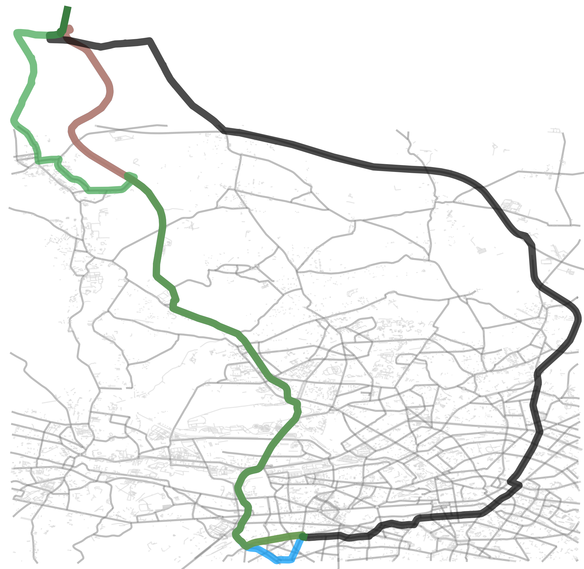
Figure 6: Visualization of example routes: Original route (blue), and optimal alternative routes for the SAP problem with respect to System Optimum (black), User Equilibrium (green) and Linear Model (orange).

Figure 7: Left: Overall travel time of the User Equilibrium and the Linear Model, relative to the System Optimum, depending on the demand $d$. Each data point is averaged over all OD-pairs. Right: The fraction of flow $x_{P}/d$ on the alternative route depending on the $d$ and the psychological model; again averaged over all OD-pairs.

The gain of splitting traffic also depends on the psychological model. We note that for most OD-pairs, the different psychological models lead to the same route and only differ in the amount of traffic using the alternative. However, there are examples where we actually get different routes, see, e.g., Figure 6. In this particular instance it is interesting to see that the System Optimum would require a large detour for some drivers (around $17\,\%$), which they probably would not accept without additional incentive.

To compare the models we proposed, we examine the proportion of agents using the suggested alternative route, and the resulting costs compared to the overall travel time when using the System Optimum in Figure 7. The Linear Model is configured with $c=1$. One can see in Figure 7 (left) that for increasing $d$, the User Equilibrium overall travel time approaches that of the System Optimum, indicating that the optimal alternative route of the User Equilibrium is not much worse than the System Optimum. This is supported by the similar amount of agents that are assigned by the models to the alternative route, as shown in Figure 7 (right). In contrast, the Linear Model uses the alternative route a lot more. We note that this is to be expected, as discussed in Section 4.

7 Conclusion

Besides providing a framework for formalizing strategic routing scenarios, we gave different algorithms solving SAP. Both of these contributions open the door to future research. Concerning SAP, we have seen that different psychological models can lead to different alternative routes, and it would be interesting to study how people actually behave depending on the exact formulation of the suggestion and on potential additional incentives to take a longer route. It is promising to study models that lie in-between the User Equilibrium and the Linear Model. By setting, e.g., $c(x)=\tanh(a\cdot x/d)$ in the Quotient Model (Equation 2), we obtain a model that behaves like the Linear Model for small $x$ and approaches the User Equilibrium Model for larger $x$, where the constant $a$ controls how quickly that happens. We note that this choice of $c(x)$ satisfies the conditions of Theorem 15, implying that the resulting model is Pareto-conform, which makes the algorithms from Section 3 applicable. Concerning algorithmic performance, we have seen that our proof-of-concept implementation yields reasonable run times. Our implementation uses techniques such as A* to speed up computation. Beyond that, there is still potential for engineering, e.g., by employing preprocessing techniques. Beyond the SAP problem, our framework gives rise to various problems in the context of strategic routing that are worth studying algorithmically.

References

- [1] Ittai Abraham, Daniel Delling, Andrew V. Goldberg, and Renato F. Werneck. Alternative routes in road networks. Journal of Experimental Algorithmics, 18, 2013. doi:10.1145/2444016.2444019.
- [2] Hannah Bast, Daniel Delling, Andrew V. Goldberg, Matthias Müller-Hannemann, Thomas Pajor, Peter Sanders, Dorothea Wagner, and Renato F. Werneck. Route planning in transportation networks. Algorithm Engineering, 2016. doi:10.1007/978-3-319-49487-6_2.
- [3] Umang Bhaskar, Lisa Fleischer, and Elliot Anshelevich. A Stackelberg strategy for routing flow over time. Games and Economic Behavior, 92:232–247, 2015.
- [4] Vincenzo Bonifaci, Tobias Harks, and Guido Schäfer. Stackelberg routing in arbitrary networks. Mathematics of Operations Research, 35(2):330–346, 2010.
- [5] Daniel Delling. Time-dependent SHARC-routing. Algorithmica, 60(1):60–94, 2009. URL: https://doi.org/10.1007/s00453-009-9341-0, doi:10.1007/s00453-009-9341-0.
- [6] Daniel Delling and Dorothea Wagner. Pareto paths with SHARC. In Experimental Algorithms, Lecture Notes in Computer Science, page 125–136. Springer, 2009. doi:10.1007/978-3-642-02011-7_13.
- [7] Daniel Delling and Dorothea Wagner. Time-dependent route planning. In Robust and Online Large-Scale Optimization: Models and Techniques for Transportation Systems, pages 207–230. Springer, 2009. doi:10.1007/978-3-642-05465-5_8.
- [8] Ugur Demiryurek, Farnoush Banaei-Kashani, and Cyrus Shahabi. A case for time-dependent shortest path computation in spatial networks. In Proceedings of SIGSPATIAL 2010, page 474–477. ACM, 2010. doi:10.1145/1869790.1869865.
- [9] Michael R. Garey and David S. Johnson. Computers and Intractability. A Guide to the Theory of NP-Completeness. W. H. Freeman, 1979. doi:10.2307/2273574.
- [10] Pierre Hansen. Bicriterion path problems. In Multiple Criteria Decision Making Theory and Application, page 109–127. Springer, 1980. doi:10.1007/978-3-642-48782-8_9.
- [11] INRIX, Inc. INRIX Verkehrsstudie: Stau verursacht Kosten in Milliardenhöhe. INRIX Press Releases, 2020. URL: https://inrix.com/press-releases/2019%2Dtraffic%2Dscorecard%2Dgerman/.
- [12] George Karakostas and Stavros G Kolliopoulos. Stackelberg strategies for selfish routing in general multicommodity networks. Algorithmica, 53(1):132–153, 2009.
- [13] Yannis A. Korilis, Aurel A. Lazar, and Ariel Orda. Achieving network optima using Stackelberg routing strategies. IEEE/ACM Transactions on Networking, 5(1):161–173, 1997. doi:10.1109/90.554730.
- [14] Alexander Kröller, Falk Hüffner, Lukasz Kosma, Katja Kröller, and Mattia Zeni. Driver expectations towards strategic routing. Unpublished Manuscript, 13 Pages.
- [15] Ekkehard Köhler, Rolf H. Möhring, and Martin Skutella. Traffic networks and flows over time. In Algorithmics of Large and Complex Networks: Design, Analysis, and Simulation, volume 5515 of Lecture Notes in Computer Science, page 166–196. Springer, 2009. doi:10.1007/978-3-642-02094-0_9.
- [16] Lawrence Mandow and José. Luis Pérez De La Cruz. Multiobjective A* search with consistent heuristics. Journal of the ACM, 57(5):27:1–27:25, 2008. doi:10.1145/1754399.1754400.
- [17] Ernesto Queirós Vieira Martins. On a multicriteria shortest path problem. European Journal of Operational Research, 16(2):236–245, 1984. doi:10.1016/0377-2217(84)90077-8.
- [18] Matthias Müller-Hannemann and Karsten Weihe. Pareto shortest paths is often feasible in practice. In Algorithm Engineering, page 185–197. Springer, 2001.
- [19] Giacomo Nannicini, Daniel Delling, Dominik Schultes, and Leo Liberti. Bidirectional A* search on time-dependent road networks. Networks, 59(2):240–251, 2011. doi:10.1002/net.20438.
- [20] US Bureau of Public Roads. Office of Planning. Urban Planning Division. Traffic Assignment Manual for Application with a Large, High Speed Computer. US Department of Commerce, 1964.
- [21] Andreas Paraskevopoulos and Christos D. Zaroliagis. Improved alternative route planning. In Proceedings of ATMOS 2013, pages 108–122. Schloss Dagstuhl, 2013. doi:10.4230/OASIcs.ATMOS.2013.108.
- [22] Tim Roughgarden. Selfish routing and the price of anarchy. MIT Press, 2005.
- [23] Tim Roughgarden and Éva Tardos. How bad is selfish routing? Journal of the ACM, 49(2):236–259, Mar 2002. doi:10.1145/506147.506153.
- [24] Leon Sering and Martin Skutella. Multi-source multi-sink Nash flows over time. In Proceedings of ATMOS 2018, pages 12:1–12:20, 2018. doi:10.4230/OASIcs.ATMOS.2018.12.
- [25] Socrates2.0. Amsterdam pilot site launched with improved navigation service. Website, Dec 2019. https://socrates2.org/news-agenda/amsterdam-pilot-launched-improved-navigation-service-testers-sought.
- [26] Ben Strasser. Dynamic time-dependent routing in road networks through sampling. In Proceedings of ATMOS 2017, pages 3:1–3:17. Schloss Dagstuhl, 2017. doi:10.4230/OASIcs.ATMOS.2017.3.
- [27] Mariska Alice van Essen. The potential of social routing advice. PhD thesis, University of Twente, 2018. doi:10.3990/1.9789055842377.
- [28] John Glen Wardrop. Some theoretical aspects of road traffic research. Proceedings of the Institution of Civil Engineers, 1(3):325–362, 1952. doi:10.1680/ipeds.1952.11259.
- [29] Michael A. Yukish. Algorithms to Identify Pareto Points in Multi-Dimensional Data Sets. PhD thesis, Mechanical Engineering Dept., The Pennsylvania State University, State College, 2004.
- [30] Shanjiang Zhu and David Levinson. Do people use the shortest path? An empirical test of Wardrop’s first principle. PLOS ONE, 10(8):1–18, 2015. doi:10.1371/journal.pone.0134322.