Importance subsampling for power system planning under multi-year demand and weather uncertainty

Abstract

This paper introduces a generalised version of importance subsampling for time series reduction/aggregation in optimisation-based power system planning models. Recent studies indicate that reliably determining optimal electricity (investment) strategy under climate variability requires the consideration of multiple years of demand and weather data. However, solving planning models over long simulation lengths is typically computationally unfeasible, and established time series reduction approaches induce significant errors. The importance subsampling method reliably estimates long-term planning model outputs at greatly reduced computational cost, allowing the consideration of multi-decadal samples. The key innovation is a systematic identification and preservation of relevant extreme events in modeling subsamples. Simulation studies on generation and transmission expansion planning models illustrate the method’s enhanced performance over established “representative days” clustering approaches. The models, data and sample code are made available as open-source software.

I Introduction

I-A Demand and weather uncertainty and computational complexity in power system planning models

Many power system planning models estimate optimal electricity investment strategy by minimising a cost function given techno-economic assumptions and constraints [1]. The use of demand and weather time series inputs (e.g. hourly load levels and wind speeds) induces forward propagated demand and weather uncertainty in model outputs, particularly when variable renewable (VR) generation such as solar and wind is considered [2]. This is because an input time series may be viewed as a sample from some underlying demand and weather distribution, and a different sample, leading to different outputs, is equally valid.

Recent studies indicate that inter-annual climate/weather variability induces considerable output uncertainty in planning models. For example, optimal system design may depend strongly on what year of data is used [3, 4, 5, 6, 7], with some optimal capacities differing as much as 80% [8, 9]. Hence, to reliably determine long-term optimal electricity strategy, multiple years of demand and weather data should be considered.

At the same time, using long samples of time series input data is unfeasible in many power system planning models due to the computational complexity in solving the associated optimisation problem [10]. This effect is amplified since accurately modeling VR generation requires a high temporal and spatial resolution, precluding an increase in step length to reduce the number of time steps [11, 12, 13].

I-B Time series reduction and subsampling

Power system modelers employ various schemes to reduce temporal complexity, as discussed in detail in [14]. A popular approach involves subsampling, often by clustering, into a smaller number of representative periods (typically days) that seek to encode longer time series in reduced form [15, 16, 17, 18, 19].

Most such reduction approaches are what the authors of [14] call a priori (or input-based) in that they depend only on the input time series but not on the underlying power system model. For example, clustering the same demand and weather data generates the same representative days (ignoring any randomness in the clustering algorithm) irrespective of whether these days are subsequently used in a highly renewable system or a system with only fossil fuel generation. In constrast, a posteriori methods use knowledge of the model’s structure or an estimate of its results. As an example, in [20], the authors run a planning model on each day individually and aggregate days by clustering (with additional modifications) the vectors of associated investment costs (model outputs). In this way, they use a subsample tailored to the model in question.

Many time series aggregation methods, such as clustering, replace individual periods/days by a group average. This “smoothes out” extremes and may lead to (1) overly optimistic predictions of system costs and (2) system design estimates that are not robust to such events. For example, such approaches may underestimate the amount of required backup generation capacity in events with high demand but low renewable generation, leading to systems with a high risk of blackouts [14]. For this reason, users sometimes make a priori heuristic adjustments such as including the maximum demand day [8].

I-C This paper’s contribution

This paper generalises significantly a version of the importance subsampling method for time series reduction/aggregation originally introduced in [9]. The contribution is as follows. Section I-A indicates that long demand and weather samples should be considered for robust power system planning under climate/weather variability, but that this is computationally challenging. Furthermore, time series reduction methods that remove extremes (Section I-B) lead to inaccurate estimates of optimal electricity strategy. The importance subsampling method systematically identifies such extremes in the full time series and includes them in a subsample, allowing reliable estimation of optimal multi-year electricity strategy at greatly reduced computational cost. A simulation study demonstrates the method’s improved performance over established clustering methods. The models, data and sample code for the method are available at [21].

This paper extends the approach introduced in [9] to almost general cost-minimisation based power system planning models. The requirements for the original method (analytical formula for generation cost, no link between time steps) restricted applications to models solvable using the (net) load duration curve. These stipulations are all relaxed. Furthermore, the generalised method allows, in addition to sampling individual time steps, the sampling of representative periods such as days or weeks (hence allowing for consideration of intra-period temporal dependencies) and uses clustering to leverage off their extensive use in power system applications.

This paper is structured as follows. Section II introduces the method and the intuition behind its working. Section III provides a case study of the method’s appliction to two generation and expansion planning (GTEP) models. Section IV discusses results and recommends extensions.

II Importance subsampling

II-A Overview and intuition

This paper considers planning models that determine optimal system design $\mathbf{D}_{\text{opt}}$ (e.g. installed capacities of generation and transmission technologies) given some (possibly weighted) demand and weather data. The model $\text{PSM}_{\text{plan}}$ is viewed as a function from a sample $\mathcal{T}$ (of length $|\mathcal{T}|$) of demand and weather data to $\mathbf{D}_{\text{opt}}$:

$$\mathbf{D}_{\text{opt}}=\text{PSM}_{\text{plan}}(\mathcal{T}).$$ (1)

The model can also run in operational mode, in which a design $\mathbf{D}$ is specified and the optimal system operation, typically with the lowest generation cost, is determined:

$$(O_{1},\ldots,O_{|\mathcal{T}|})=\text{PSM}_{\text{operate}}(\mathcal{T}|\mathbf{D}).$$ (2)

Here, $O_{t}$ is the power system operation (generation and transmission levels) at time $t$, for each time step $t=1,\ldots,|\mathcal{T}|$. In many planning models (e.g. ones that seek the design minimising the sum of build costs and subsequent minimum generation costs), the operational model is solved as a subproblem. However, this is not necessary for the proposed method.

The setup is then as follows. Suppose $\mathcal{T}$ is a contiguous sample of demand and weather data and the associated optimal system design $\mathbf{D}_{\text{opt}}$, as defined by (1), is desired. If $\mathcal{T}$ is long, solving the optimisation problem to determine $\mathbf{D}_{\text{opt}}$ may be computationally unfeasible. The importance subsampling method instead estimates $\mathbf{D}_{\text{opt}}$ by running the planning model across a shorter (weighted) subsample of time series data $\mathcal{S}$. An estimate of $\mathbf{D}_{\text{opt}}$ in (1) is hence provided by

$$\mathbf{D}_{\text{opt}}^{\mathcal{S}}:=\text{PSM}_{\text{plan}}(\mathcal{S}).$$ (3)

The goal is that $\mathbf{D}_{\text{opt}}^{\mathcal{S}}\approx\mathbf{D}_{\text{opt}}$ with $|\mathcal{S}|<|\mathcal{T}|$, so that optimal system design is reliably estimated at reduced computational cost. The key is hence how the sample $\mathcal{S}$ is created.

The importance subsampling method works by explicitly including a selection of “extreme” events in a modeling subsample. In this paper, “extreme” refers to time steps in which meeting demand requires a large amount of generation or transmission capacity. In many planning models, omitting such extremes leads to inaccurate estimates of optimal system design (e.g. underestimation of required backup generation capacity, see Section I-A). It is hence essential that such events are identified and preserved when subsampling. At the same time, identifying them a priori is difficult since which time steps are “extreme” may depend on the system design being estimated. As a simple example, in a model containing an unknown wind generation capacity, it is unclear whether a 55MW demand, 0.1 wind capacity factor time step is more “extreme” (in the sense of requiring more backup capacity) than one with 60MW demand and 0.2 wind capacity factor.

Importance subsampling systematically identifies relevant extremes using their importance, calculated using the user-defined function IMP (see Section II-B). This function should be a proxy for how “extreme” a time step is. In many applications (e.g. Section III), a time step’s generation cost performs well since expensive measures (e.g. peaking plants or load curtailment) are activated only in scenarios when there is otherwise a supply shortage. Other choices are possible; electricity price is another candidate in models with such a notion. In practice, expert knowledge of the system should motivate a choice of importance function.

Determining each time step’s importance generally requires the associated generation and transmission levels, determined by running the model in operational mode with some fixed design. Ideally, importance levels are calculated using the true optimal system design, but this is the output being estimated and hence unknown. For this reason, a preliminary planning model run with a standard subsampling scheme is used for a rough estimate of optimal system design. This is subsequently used to determine the importance of each time step in the full time series.

At a high level, the approach works as follows (with correspondence to Section II-B shown in parantheses):

1. Estimate optimal system design through model run with standard subsampling (a priori) procedure (steps 1-2).

2. Using this estimate, calculate importance for each time step in full time series. In general, this requires running the model in operational mode (steps 3-4).

3. Create importance subsample by subsampling again while explicitly preserving the relevant extreme events (those with high importance) (step 5).

A model is subsequently run with the importance subsample $\mathcal{S}$ to estimate optimal system design.

II-B Algorithm

Algorithm: Importance subsampling
Inputs:

• $\mathcal{T}$: full time series to sample from, of length $|\mathcal{T}|$

• $n_{d}$: number of days to sample

• $n_{d_{e}}$: number of “extreme” days to sample

Steps:

1. Cluster full time series into $n_{d}$ weighted representative days to create $\mathcal{C}$.

2. Run planning model to determine $\mathbf{D}_{\text{opt}}^{\mathcal{C}}$, the cluster estimates of optimal system design:

   $$\mathbf{D}_{\text{opt}}^{\mathcal{C}}=\text{PSM}_{\text{plan}}(\mathcal{C}).$$ (4)

3. Determine system operation $(O_{1}^{\mathcal{C}},\ldots,O_{|\mathcal{T}|}^{\mathcal{C}})$ (generation and transmission levels at each time in $\mathcal{T}$) by running model in operational mode with design $\mathbf{D}_{\text{opt}}^{\mathcal{C}}$:

   $$(O_{1}^{\mathcal{C}},\ldots,O_{|\mathcal{T}|}^{\mathcal{C}})=\text{PSM}_{\text{operate}}(\mathcal{T}|\mathbf{D}_{\text{opt}}^{\mathcal{C}}).$$ (5)

4. Assign each time step its importance:

   $$\text{imp}_{t}=\text{IMP}(O_{t}^{\mathcal{C}})\quad\forall t\in\mathcal{T}.$$ (6)

   for user-defined IMP function (see Section II-A).

5. Create $n_{d}$-day importance subsample $\mathcal{S}$ containing:

   • $n_{d_{e}}$ most “extreme” days in $\mathcal{T}$ as ranked by the importance of their highest time step.

   • $n_{d}-n_{d_{e}}$ days obtained by clustering the remainder of the full time series.

   Weight days to account for their proportion across the full time series $\mathcal{T}$ (see Section II-C).

Outputs:

• $\mathcal{S}$: weighted importance subsample

II-C Remarks

The proposed method is an a posteriori time series aggregation scheme that customises the subsample to the model. Most established time series reduction methods (Section I-A) are a priori schemes which do not use knowledge of the underlying model. This corresponds to following just step i in Section II-A (steps 1-2 in Section II-B) and using $\mathbf{D}_{\text{opt}}^{\mathcal{C}}$ as the final estimate. Importance subsampling instead uses this estimate to create an additional customised sample to provide a second, more accurate, estimate of optimal system design.

Estimating optimal system design using importance subsampling requires three model runs (with correspondence to Section II-B shown in parantheses):

1. Preliminary planning model run on $n_{d}$ days (step 2)

2. Operational model run with fixed capacities on full time series (step 3)

3. Planning model run on $n_{d}$-day importance subsample.

The first and third runs are planning models that determine optimal system design. These models usually also determine the associated optimal generation levels as part of the optimisation problem, but this output is ignored. In contrast, the second run determines just the system’s operation with a fixed design. Operational models’ solution times typically scale linearly in the number of time steps and are much shorter than for planning models [22]. For this reason, a planning model run with importance subsample requires roughly twice the computational time as a single planning model run across $n_{d}$ days.

The importance subsample is weighted to account for the relative proportions of days throughout the full time series. For example, the 30 most extreme days in a 30-year sample represent one day a year, but will represent 30 days a year if all included a 1-year subsample. The time steps are hence weighted to avoid the estimated optimal system design being over-engineered for extreme events. The $n_{d}-n_{d_{e}}$ non-extreme days are weighted according to their cluster sizes.

The clustering/subsampling algorithms used in steps 1 and 5 of Section II-B are customisable. Furthermore, periods other than days may be sampled. The advantage of sampling longer periods (e.g. weeks) is that it respects long-term temporal dependencies such as storage to a greater degree. The advantage of sampling shorter blocks is that the total number of periods in a fixed-length subsample is larger, meaning a higher diversity of possible demand and weather scenarios is considered. Hence, the choice of subsample blocks is a tradeoff between a high diversity of scenarios and a low distortion of time step chronology. In models without temporal dependencies, randomly sampling individual time steps (without any clustering) typically gives the best results, but longer periods should be selected in models with ramping or storage constraints.

III Simulation studies

III-A Overview

This section examines the efficacy of the proposed method on sample power system planning models. This is done by comparing optimal system design across importance subsamples with that across the full time series from which samples are drawn. As a benchmark, the model is also run across samples generated by $k$-medoids clustering, representing the current industry standard. The reason for choosing $k$-medoids clustering (where the real day closest to the cluster mean is used as the representative day, instead of the mean itself) is its widespread use in previous studies and that it typically performs better than $k$-means [14], which smooths out extremes by using the cluster mean.

Two metrics indicating the “degree of suboptimality” of estimated system design (compared with the true optimum across the full time series) are also calculated:

• Peak capacity shortage: maximum value of demand minus available generation capacity, in MW.

• Energy unserved: (annualised) demand impossible to meet with generation capacity, in MWh/yr. Can be turned into monetary value via a value of lost load.

These metrics are determined by running a model, with design estimated across subsamples, in operational mode across the full time series.

III-B Power system planning models

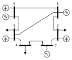
Bus	Demand/candidate generation
1	baseload, peaking
2	demand (DE), wind (DE)
3	baseload, peaking
4	demand (FR)
5	demand (UK), wind (UK)
6	baseload, peaking, wind (ES)

Figure 1: Power system planning model configuration. Time-varying demand is met at buses 2, 4 and 5. Thermal generation (baseload or peaking) may be built at buses 1, 3 and 6, while wind power may be installed at buses 2, 5 and 6. Time series input data are aggregated demand and wind levels for Germany (DE), France (FR), United Kingdom (UK) and Spain (ES).

The method is tested on two (generation and transmission expansion) planning models with topologies equal to a renewables-containing version of the IEEE 6-bus system originally introduced in [23, 24]. Optimal system design (generation and transmission capacities across the grid) is determined by minimising the total system cost (sum of install and generation costs) given hourly demand levels and wind capacity factors. The model determines the optimal capacity and generation mix across baseload, peaking and wind technologies. Time series input data consists of hourly demand levels and wind capacity factors in European countries, introduced in [25, 26]. An overview of the model’s topology is provided in Fig. 1. The models and time series data are publicly available at [27], where their mathematical formulations are described.

The two models differ in the complexity of their constraints. The first, the LP model, is a linear program (LP) in which technologies may be installed to any nonnegative capacity and there is no intertemporal dependence between time steps. In the MILP model, baseload capacity is constrained to blocks of 3GW and a ramp rate of 20%/hr, making the model a mixed-integer linear program (MILP) with ramping constraints.

III-C Simulation setup

TABLE I: Simulations in Section III-D. $n_{d_{e}}$ is the number of “extreme” days included in subsamples. For importance subsampling, solution times are disaggregated into first planning run, operational run and second planning run.

Time series data			Mean solution requirements
	length $n_{d}$	$n_{d_{e}}$	Time	Memory
Subsampling	(days)	(days)	(min)	(MB)
LP model, full time series 2008-2017
None (target)	3650	-	340	15121
$k$-medoids	48	-	0.5	393
importance	48	16	0.5+11+0.5	742
$k$-medoids	90	-	1	567
importance	90	30	1+11+1	753
MILP model, full time series 2017
None (target)	365	-	2926	1598
$k$-medoids	24	-	2	270
importance	24	8	2+2+2	823
$k$-medoids	48	-	9	362
importance	48	16	9+2+9	841

Details for the simulations are provided in Table I. For the LP model, optimal design across 2008-2017 serves as the target for simulations with $n_{d}$=48 and 90-day subsamples. For the MILP model, the integer constraints impose (much) longer solution times and the optimal design across 2017 is estimated using subsamples of length $n_{d}$=24 and 48 days. Since both $k$-medoids clustering and importance subsampling contains randomness from the initialisation of cluster means, the distribution of model outputs across 100 subsamples is determined. Computational times are based on model runs created in the open-source energy modeling framework Calliope [22] and solved using the cbc [28] solver on a 2.7GHz Intel Core i5-5257U processor with 8GB of RAM (with some additional “swap” memory available).

The implementation of the importance subsampling method (Section II-B) is as follows. $k$-medoids clustering is used in steps 1 and 5. Each time series is normalised to lie between 0 and 1 (so that demand levels and wind capacity factors can be compared fairly), but no additional adjustments are made. For the importance function in step 4, a time step’s generation cost (sum of each technology’s generation cost times generation level) is used since expensive technologies with high generation cost (e.g. peaking plants) are used only in “extreme” scenarios when blackouts would occur otherwise. For $n_{d_{e}}$, the number of “extreme” days containing the highest generation costs, a value of $n_{d_{e}}=\frac{1}{3}n_{d}$ is used as this gives good results in practice, balancing the need to capture a range of “extreme” events while leaving enough of the sample to accurately approximate the more typical days.

III-D Results

LP model, full time series 2008-2017
(a) $n_{d}$=48-day subsample, $n_{d_{e}}$=16 “extreme” days

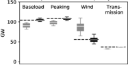
(b) $n_{d}$=90-day subsample, $n_{d_{e}}$=30 “extreme” days

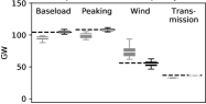
MILP model, full time series 2017
(c) $n_{d}$=24-day subsample, $n_{d_{e}}$=8 “extreme” days

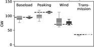
(d) $n_{d}$=48-day subsample, $n_{d_{e}}$=16 “extreme” days

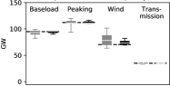
Figure 2: Distribution of estimated optimal capacities and suboptimality metrics (peak capacity shortage, energy unserved) across 100 samples generated by $k$-medoids clustering and importance subsampling. The box-and-whiskers show the 2.5%, 25%, median, 75% and 97.5% percentiles. The optima across the full time series (targets) are shown as a dashed black line.

Fig. 2 shows the distribution of estimated optimal capacities and suboptimality metrics (peak capacity shortage, energy unserved) across the test simulations. For the same plots among the full range of model outputs (at regional level) and for a larger number of sample sizes, including sampling individual hourly time steps instead of days, visit [21]. Importance subsampling into representative days generally has superior performance to $k$-medoids clustering, with more accurate estimates of optimal system design, lower levels of capacity shortage and energy unserved, and lower variability in model outputs. For example, $k$-medoids clustering usually underestimates (overestimates) optimal peaking (wind) capacity, but such biases are not present for importance subsampling. As a result, levels of capacity shortage and unmet demand across the full time series (rightmost two columns) are lower (almost 0) for importance subsampling than for $k$-medoids. A system designed based on 48 representative days $k$-medoids clustered from 10 years (Fig. 1(a)) fails to meet 0.05% of demand on average, compared to virtually none for a system designed using importance subsampling. This has financial implications; assigning a value of lost load of $\pounds$6000/MWh [29] implies an increase in system cost of around 1% per each 0.01% of demand that is unmet. In summary, importance subsampling provides estimates of optimal system design that are both more accurate (estimated optimal capacities are closer to the true optimum across the full time series) and more robust to extreme events (much lower levels of capacity shortage and unserved energy).

III-E Discussion

The superior performance of importance subsampling is a direct result of the method’s explicit preservation of extreme days. By design, $k$-medoids clustering is equivalent to using $\mathcal{C}$ in step 1 (Section II-B) to generate the final estimates of optimal system design. Hence, the improved performance of importance subsampling comes only from steps 2-5, in which extreme days are identified and included. It is to be expected that the failure to include these events results in the underestimation (overestimation) of peaking (wind) capacity observed in Fig. 1; samples not including high demand, low wind events underestimate the amount of required backup generation capacity while overestimating the reliability of wind power.

The performance gap of importance subsampling over $k$-medoids clustering appears more strongly when subsampling from longer time series, as seen by comparing Fig. 2(a) and (d). This is because representing a shorter time series (with a smaller range of extreme events) using e.g. clustering is easier than doing the same (with equal subsample size) for a longer, more diverse time series. Hence, the added value of importance subsampling is expected to grow as longer time series (e.g. multiple decades) are sampled from.

The importance subsampling method can estimate model outputs from simulations much longer than those used here. For example, it is possible to estimate a 25-year output by a 1-year subsample. The use of shorter samples is only to make validation of the method possible by comparing with the “ground truth” determined by a brute force model run on the full time series. The use of short samples in this manner has also distorted the computational expense. In most realistic planning models, computational expense for importance subsampling is dominated by the two planning runs. This is because solution times for the operational model scale linearly in the number of time steps while that for a planning run scales faster. For example, for the MILP model, a 1-year estimate of 25-year optimal design requires around 48 hours for each planning run but just 48 minutes for the operational run across the full 25 years.

IV Conclusions

This paper’s main contribution is a significant generalisation of the importance subsampling method. This approach can reliably estimate long-term planning model outputs (considering multiple decades of demand and weather data) at greatly reduced computational cost, outperforming industry standard a priori time series aggregation methods. As discussed in Section I-A, the consideration of such long samples is essential for robust power system planning under natural climate/weather variability. This method also allows the consideration of climate model data in power system planing (see e.g [30, 31, 32]), where differences in climate have a weak signal-to-noise ratio under natural variability and hence require long samples to identify statistically significant effects. The models, data and sample code are available at [21].

The key innovation behind the proposed methodology is a systematic identification and inclusion of relevant “extreme” events in subsamples through a user-defined importance function. This function may be tailored to the specific application, but in many settings a time step’s generation cost or electricity price will suffice (Section II-C). The systematic identification of relevant extremes may also be used in its own right, for example by using the identified “extreme” days for subsequent reliability analysis at higher spatiotemporal resolution.

Importance subampling is an a posteriori method (see Section I-B) in which properties of the model and/or its results are used to improve time series aggregation. The method can be compared with that in [20], where the time series aggregation is performed, along with a number of other modifications, across the vectors of model outputs (costs at technological and regional levels) for each individual day. This is another promising approach to a similar problem. Importance subsampling is simpler, though a more thorough comparison of the two methods would be interesting.

Two potential extensions to the method are further refinements to model interdependence between the sampled days (as in e.g. weekly/seasonal storage), and dimensionality reduction when the number of grid locations becomes very large.

References

- [1] A. Bazmi and G. Zahedi, “Sustainable energy systems: Role of optimization modeling techniques in power generation and supply — a review,” Renew. Sust. Energy Rev., vol. 15, no. 8, pp. 3480–3500, 2011.
- [2] A. P. Hilbers, D. J. Brayshaw, and A. Gandy, “Efficient quantification of the impact of demand and weather uncertainty in power system models,” arXiv e-prints, p. arXiv:1912.10326, 2019.
- [3] H. C. Bloomfield, D. J. Brayshaw, L. Shaffrey, P. Coker, and H. Thornton, “Quantifying the increasing sensitivity of power systems to climate variability,” Environ. Res. Lett., vol. 11, p. 124025, 2016.
- [4] M. Zeyringer, J. Price, B. Fais, P.-H. Li, and E. Sharp, “Designing low-carbon power systems for Great Britain in 2050 that are robust to the spatiotemporal and inter-annual variability of weather,” Nature Energy, vol. 3, pp. 395–403, 2018.
- [5] I. Staffell and S. Pfenninger, “The increasing impact of weather on electricity supply and demand,” Energy, vol. 145, pp. 65–78, 2018.
- [6] S. Collins, P. Deane, B. Ó Gallachóir, S. Pfenninger, and I. Staffell, “Impacts of inter-annual wind and solar variations on the European power system,” Joule, vol. 2, no. 10, pp. 2076 – 2090, 2018.
- [7] C. Bothwell and B. F. Hobbs, “Sensitivity of resource adequacy to sample error in systems with dependent renewable generation,” in Proc. 16th Int. Conf. PMAPS, June 2018, pp. 1–6.
- [8] S. Pfenninger, “Dealing with multiple decades of hourly wind and PV time series in energy models: a comparison of methods to reduce time resolution and the planning implications of inter-annual variability,” Applied Energy, vol. 197, pp. 1–13, 2017.
- [9] A. P. Hilbers, D. J. Brayshaw, and A. Gandy, “Importance subsampling: improving power system planning under climate-based uncertainty,” Applied Energy, vol. 251, p. 113114, 2019.
- [10] H.-K. Ringkjøb, P. M. Haugan, and I. M. Solbrekke, “A review of modelling tools for energy and electricity systems with large shares of variable renewables,” Renew. Sust. Energy Rev., vol. 96, pp. 440 – 459, 2018.
- [11] K. Poncelet, E. Delarue, D. Six, J. Duerinck, and W. D’haeseleer, “Impact of the level of temporal and operational detail in energy-system planning models,” Applied Energy, vol. 162, pp. 631 – 643, 2016.
- [12] S. Collins, J. P. Deane, K. Poncelet, E. Panos, R. C. Pietzcker, E. Delarue, and B. Ó Gallachóir, “Integrating short term variations of the power system into integrated energy system models: A methodological review,” Renew. Sust. Energy Rev., vol. 76, pp. 839 – 856, 2017.
- [13] L. Kotzur, P. Markewitz, M. Robinius, and D. Stolten, “Impact of different time series aggregation methods on optimal energy system design,” Renew. Energy, vol. 117, pp. 474–487, 2018.
- [14] M. Hoffmann, L. Kotzur, D. Stolten, and M. Robinius, “A review on time series aggregation methods for energy system models,” Energies, vol. 3, no. 13, p. 641, 2020.
- [15] D. Fitiwi, F. de Cuadra, L. Olmos, and M. Rivier, “A new approach of clustering operational states for power network expansion planning problems dealing with RES (renewable energy source) generation operational variability and uncertainty,” Energy, vol. 90, pp. 1360 – 1376, 2015.
- [16] P. Nahmmacher, E. Schmid, L. Hirth, and B. Knopf, “Carpe diem: a novel approach to select representative days for long-term power system modeling,” Energy, vol. 112, pp. 430–442, 2016.
- [17] P. Härtel, M. Kristiansen, and M. Korpås, “Assessing the impact of sampling and clustering techniques on offshore grid expansion planning,” Energy Proc., vol. 137, pp. 152–161, 2017.
- [18] K. Poncelet, H. Höschle, E. Delarue, A. Virag, and W. D’haeseleer, “Selecting representative days for capturing the implications of integrating intermittent renewables in generation expansion planning problems,” IEEE Trans. Power Syst., vol. 32, pp. 1936–1948, 2017.
- [19] D. A. Tejada-Arango, M. Domeshek, S. Wogrin, and E. Centeno, “Enhanced representative days and system states modeling for energy storage investment analysis,” IEEE Trans. Power Syst., vol. 33, no. 6, pp. 6534–6544, 2018.
- [20] M. Sun, F. Teng, X. Zhang, G. Strbac, and D. Pudjianto, “Data-driven representative day selection for investment decisions: A cost-oriented approach,” IEEE Trans. Power Syst., vol. 34, no. 4, pp. 2925–2936, July 2019.
- [21] A. P. Hilbers, “ahilbers/importance_subsampling: PMAPS paper version,” May 2020. [Online]. Available: https://doi.org/10.5281/zenodo.3841154
- [22] S. Pfenninger and B. Pickering, “Calliope: a multi-scale energy systems modelling framework,” Journal of Open Source Software, vol. 3(29), p. 825, 2018.
- [23] S. Kamalinia and M. Shahidehpour, “Generation expansion planning in wind—thermal power systems,” IET Generation, Transmission & Distribution, vol. 4-8, pp. 940–951, 2010.
- [24] S. Kamalinia, M. Shahidehpour, and A. Khodaei, “Security-constrained expansion planning of fast-response units for wind integration,” Elec. Power Syst. Res., vol. 81, no. 1, pp. 107 – 116, 2011.
- [25] H. C. Bloomfield, D. J. Brayshaw, and A. Charlton-Perez, “Characterising the winter meteorological drivers of the European electricity system using targeted circulation types,” Meteorol. Appl., 2019.
- [26] ——, “MERRA2 derived time series of European country-aggregate electricity demand, wind power generation and solar power generation,” 2020, dataset. [Online]. Available: dx.doi.org/10.17864/1947.239
- [27] A. P. Hilbers, “ahilbers/renewable_test_psms: Paper version,” May 2020. [Online]. Available: https://doi.org/10.5281/zenodo.3841171
- [28] johnjforrest, S. Vigerske, H. G. Santos, T. Ralphs, L. Hafer, B. Kristjansson, jpfasano, EdwinStraver, M. Lubin, rlougee, jpgoncal1, h-i gassmann, and M. Saltzman, “coin-or/cbc: Version 2.10.5,” Mar. 2020. [Online]. Available: https://doi.org/10.5281/zenodo.3700700
- [29] E. Bucaj, “Value of lost load review process,” Elexon, Technical Report., 2018. [Online]. Available: https://www.elexon.co.uk/wp-content/uploads/2017/09/33_278_10_VoLL-Review-Process-Paper-v1.0.pdf
- [30] J. Wohland, M. Reyers, J. Weber, and D. Witthaut, “More homogeneous wind conditions under strong climate change decrease the potential for inter-state balancing of electricity in Europe,” Earth Syst. Dynam., vol. 8, no. 4, pp. 1047–1060, Nov 2017.
- [31] M. T. Craig, I. L. Carreño, M. Rossol, B.-M. Hodge, and C. Brancucci, “Effects on power system operations of potential changes in wind and solar generation potential under climate change,” Environ. Res. Lett., vol. 14, no. 3, p. 034014, mar 2019.
- [32] B. Van Zuijlen, W. Zappa, W. Turkenburg, G. van der Schrier, and M. Van den Broek, “Cost-optimal reliable power generation in a deep decarbonisation future,” Applied Energy, vol. 253, p. 113587, 2019.