Bosch Deep Learning Hardware Benchmark

Abstract

The widespread use of Deep Learning (DL) applications in science and industry has created a large demand for efficient inference systems. This has resulted in a rapid increase of available Hardware Accelerators (HWAs) making comparison challenging and laborious. To address this, several DL hardware benchmarks have been proposed aiming at a comprehensive comparison for many models, tasks, and hardware platforms.

Here, we present our DL hardware benchmark which has been specifically developed for inference on embedded HWAs and tasks required for autonomous driving. In addition to previous benchmarks, we propose a new granularity level to evaluate common submodules of DL models, a twofold benchmark procedure that accounts for hardware and model optimizations done by HWA manufacturers, and an extended set of performance indicators that can help to identify a mismatch between a HWA and the DL models used in our benchmark.

I Introduction

Deep learning hardware benchmarks are of vital importance for the evaluation and comparison of DL HWAs due to the rapidly evolving number of DL models and accelerators. We are currently tracking a list of over 200 HWAs, which keeps growing on a weekly basis. A major challenge for customers of these accelerators is the need for a use-case specific evaluation and comparison. For instance, the requirements of small image classification (e.g. ImageNet [1]) vastly differ from those of 4k image semantic segmentation. This applies to both number of computations and memory accesses as well as to the building blocks used in these DL models. Therefore, Bosch has developed its own DL hardware benchmark. This benchmark focuses on the inference phase of embedded HWAs and reflects the particular requirements of computer vision applications, such as those of autonomous driving visualized in Fig. 1.

In recent months, industry standards for DL hardware benchmarks appear to become increasingly established. This is needed in order to cope with the increasing number of both DL models and HWAs and to keep the effort for both hardware vendors and customers at an acceptable level. In addition to enabling an evaluation, we see benchmarks as a tool to communicate industry requirements to hardware vendors.

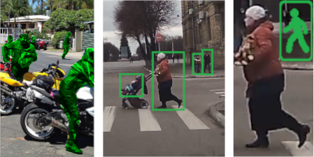
Figure 1: Examples visualizing the three tasks considered in our benchmark (from left to right): semantic segmentation, object detection, and action recognition. In addition to task-specific benchmarks, we include the novel concept of feature extractor benchmarks.

In this paper we describe the reasoning behind our benchmark design, and propose to use this as a starting point for further contributions to public benchmarks and industry standards. We are convinced that our benchmark contains several novel aspects of interest to the community. Besides the general model selection, our main benchmark design contributions are the following:

• A combination of model-level, also referred to as macro-level, benchmarks in addition to feature-extractor benchmarks, hereinafter also referred to as meso-level benchmarks.

• A twofold benchmark procedure based on unoptimized benchmarks, allowing a direct evaluation of certain DL structures and building blocks, in addition to optimized benchmarks, allowing an evaluation of the optimization capabilities in both hardware, but especially also in the corresponding software tools.

• An extensive list of performance indicators, thus enabling partial cross-validation.

However, we will not be able to share results of specific HWAs due to confidentiality.

The remainder of this paper is structured as follows: we summarize related work in Section II and then give a general overview of design considerations and decisions in Section III. The benchmark structure and included models are presented in Section IV. Our evaluation procedure (see Fig. 2) and the used performance indicators are addressed in Section V before concluding in Section VI.

Figure 2: Benchmark roll-out and evaluation procedure that is conducted in a cooperation with each hardware vendor.

II Related Work

As many DL hardware benchmarks already exist [2], we provide a brief overview of similar benchmarks in chronological order:

Fathom [3], already published in 2016, is one of the first DL hardware benchmarks. It consists of eight models which cover tasks ranging from sentence translation to Atari-playing. Another pioneer in the field of DL hardware benchmarks is Baidu’s DeepBench [4], which focuses on benchmarking of basic DL operations such as convolutions or matrix multiplications. DAWNBench [5, 6], an end-to-end DL training and inference benchmark suite, focuses on image classification and question answering. The authors recently announced that DAWNBench will stop accepting rolling submissions in favor of MLPerf (see below). The International Open Benchmark Council, a non-profit research institute, recently published several benchmark suites for different domains, including Edge AIBench [7], AIoTBench [8], and AIBench [9]. The number of benchmarks included in these suites is enormous and the benchmarks cover different granularity levels, different tasks, and domain specific application tests. Application specific benchmarks for the automotive domain have been developed by EEMBC (ADASMark [10]) as well as Basemark (BATS [11]). However, as these benchmark suites are focusing on advanced driver-assistance systems (ADAS), the DL benchmarks are only a partial aspect of the complete benchmark suite. Another organization which is rapidly gaining momentum is MLPerf [12], a collaboration of companies and researchers from educational institutions. Both a training benchmark [13] and an inference benchmark exist [14], which are partly based on the same models.

III Motivation and Design

This section gives an overview of the fundamental design considerations in DL hardware benchmark design and motivates the decisions made for the Bosch Deep Learning Hardware Benchmark.

III-A Motivation

A large number of different DL hardware benchmarks exist, but each benchmark has unique characteristics and is designed for different domains and evaluation scenarios. Our focus is on evaluating only the inference performance of Deep Neural Networks (DNNs) on embedded HWAs, which considers latency, throughput, accuracy, and other important performance indicators. We do not consider acceleration of training here, since we assume this is done offline. Existing DL hardware benchmarks were not suitable for our purposes at the time of development, as (1) they did not cover all aspects relevant for us, (2) they were designed for other hardware platforms (e.g. GPUs or $\mathrm{\SIUnitSymbolMicro}$Cs), (3) they were designed for different conditions, e.g. focusing on training instead of inference.

The fact that industry wide standards seem to become established is encouraging. The rapidly increasing number of DL models and DL hardware architectures leads to a significant increase in the effort required for a fair comparison with state of the art models and datasets for both hardware vendors and customers. Industry standards offer the chance that these efforts can be bundled.

III-B Training vs. Inference

Most DL algorithms involve two consecutive stages: training and inference. During training, the model is taught to solve a task, e.g. $1000$-class image classification, on a training dataset. During inference, the model predicts the task outcome on unseen data. Since the model is typically not changed anymore during inference, training and inference can be treated independently and may thus generally be conducted on different hardware with potentially strongly differing characteristics. In our benchmark we only focus on inference.

III-C Granularity

One fundamental design consideration of every DL hardware benchmark is its granularity, i.e. at which level benchmarks are defined. Table I shows an overview of typical benchmark granularity levels. Kernel-level benchmarks, often referred to as micro benchmarks, test single operations, such as convolutions or matrix multiplications. This enables a direct evaluation of the tested kernel operations and their parameters. Next are layer-level benchmarks, which test individual network layers, providing an analogous evaluation. The most common benchmark category is at model-level, also referred to as macro level. Such benchmarks are based on complete DL models, where the main advantage are measurable model accuracies and effects across layer boundaries, such as layer fusion.

Sub-model-level benchmarks are based on several layers, which do not define complete models. Specifically, they do not solve any task, which in turn does not allow a task accuracy evaluation such as classification accuracy. We refer to them as meso-level benchmarks. In this work we present how to successfully employ meso-level benchmarking to increase the expressiveness of a DL hardware benchmark.

Finally, task-level benchmarks are not limited to a concrete DL model, but only describe a task, e.g. object detection in fixed-size images. Thus, this level incurs the least restrictions, but may require comparing differing DL model implementations on different hardware architectures, thus hindering a direct comparison.

	Hardware Arch.	Fixed	Configurable	Programmable
	Flexibility	Low	Medium	High
Granularity Level	Kernel		(x)	x
	Layer		x	x
	Sub-model		x	x
	Model	(x)	x	x
	Task	x	x	x

Table I: Typical DL hardware benchmark granularities and how they suit to a coarse categorization of DL HWAs.

The above considerations clearly show that the benchmark level has to be chosen carefully depending on the specific goals. To explain this in more detail, consider three HWAs, namely one supporting a fixed DL model, a configurable one of medium flexibility and a fully programmable one. While all DL hardware benchmark levels are suitable for the latter, kernel-level benchmarks may be less suitable for the configurable HWA, as they might not be supported in an efficient manner or at all. The fixed HWA, which represents the category of ultra low power, in-memory computing based accelerators, is the least flexible and can practically only be tested with task-level benchmarks. In this case, prediction accuracy has to be evaluated carefully when comparing HWAs that support different models. Model-level benchmarks could also be supported, provided that the tested model is restricted to the native (sub-)model of the HWA.

As our benchmark is aiming for accelerators with medium to high flexibility, layer- to task-level benchmarks would be suitable. However, since we consider optimizations across layer boundaries to be crucial, we decided for a combination of model- and sub-model-level benchmarks (see Section IV).

III-D Representation

Another important aspect of a DL hardware benchmark is the representation level of the single benchmarks, i.e. how abstract a benchmark task is defined. While task-level benchmarks can be described in a textual way, benchmarks of all other levels are usually described in a reference format based on a specific DL framework, an exchange format, or an intermediate representation. Since our primary goal was to enable easy adoption for as many HWAs as possible, we decided to use TensorFlow [15]. However, some hardware vendors converted our models to other frameworks such as Caffe [16], as their deployment toolchain was optimized for it. In the future, unified representations such as ONNX [17] could be considered.

III-E Modifications and Optimizations

Several methods exist to optimize the inference of DL models, both regarding hardware (e.g. dedicated compression modules), software (e.g. kernel pruning), or a combination of both (e.g. quantization). In particular for embedded systems, which usually have strict energy, latency, and throughput requirements, those techniques are highly relevant and almost all dedicated HWAs and the corresponding software toolkits support a combination of such techniques. As several of these modify the DL model significantly, they complicate the evaluation of individual hardware features, such as the efficiency of a specific layer structure. Thus, the question arises, which techniques shall be allowed in a DL hardware benchmark.

We classify DL hardware benchmarks into four categories:

1. identical computation, i.e. the DL model is executed as supplied

2. identical computation, but quantization allowed

3. optimization techniques allowed, but without retraining

4. optimization techniques allowed including retraining

In our benchmark we allow two of these four categories. As it is designed to enable an evaluation of certain building blocks of DNNs, on the one hand, we are interested in direct results without optimization. As several embedded HWA do not support floating-point operations, we allow only quantization for non-optimized results, which corresponds to category 2.

On the other hand, we are also interested in the aforementioned optimization techniques, and in particular the capabilities of the deployment toolchain. Since our focus here is on the evaluation of the maximal optimization level, we allow all optimizations techniques, including retraining in the category optimized, corresponding to category 4. The only restriction is a model-specific tolerated accuracy degradation to avoid unreasonable optimizations.

III-F Input Resolution

Clearly, the resolution of processed images has a major impact on the absolute performance of HWAs. Many previous works only considered relatively small images, yet for automotive applications, such as object detection and semantic segmentation, a wide field of view and large sensing range are crucial, which in turn requires a high image resolution. We therefore consider images of Full HD resolution ($1920\times 1080$px), except for the Action Recognition benchmarks.

IV Benchmark Structure

In this section we describe the general benchmark structure, the ideas behind it, the selected benchmark models, and the used datasets.

IV-A Benchmark Structure Design

Our proposed benchmark is composed of two distinct, yet strongly related parts. During the last years, deep learning models have become increasingly modular. Many new network architectures have been developed in the course of ILSVRC [1], such as VGG16 [18], DenseNet [19], up to the recent EfficientNet [20]. Research has shown that combining parts of the ImageNet-pretrained network with the task-specific structure and loss can yield state-of-the-art results. We term these two elements of a CNN the feature extractor or backbone of the model, and the task-specific head. As a consequence many tasks can be approached using a wide variety of well-established feature extractors combined with the task-specific head.

This is one of the key insights we exploit in our benchmark design. In order to reduce the evaluation complexity, we provide orthogonal feature extractor benchmarks and define the task-specific benchmarks based on a single feature extractor. This allows e.g. comparing results of a MobileNet-based Single Shot Detector (SSD) [21] for object detection with a VGG-based SSD without the need for conducting this benchmark explicitly.

In the following we describe which particular feature extractors and tasks we selected for our benchmark and motivate our choices. A summary is presented in Table II.

IV-B CNN building blocks and feature extractor models

Most modern feature extractors consist of specific building blocks, which are arranged and repeated in a regular pattern [22] [23], e.g. the fire-module [24]. We will call them single-block extractors. Often each such building block incurs specific requirements on HWAs, e.g. efficient execution of $1\times 1$ convolutions. Many other feature extractors combine several differing building blocks in a beneficial way [25] [26], which we will call mixed-block extractors.

Mixed-block extractors often surpass their single-block predecessors in reported metrics, such as parameter count vs. accuracy, or FLOPs vs. accuracy. For benchmarking purposes however, mixed-block extractors pose a significant challenge. Execution capability and performance will strongly depend on the least-supported building block, which then produces uninterpretable results for complex feature extractors. Conversely, if single-block extractors are computed efficiently on a HWA, mixed-block extractors composed of the involved individual blocks are also highly likely to be computed efficiently. If they do not, the influencing factor is easily identifiable.

In the following, we describe the building blocks and feature extractor models we selected for closer investigation. Note that there are many more available in the literature.

IV-B1 Vanilla convolutions

One of the most commonly used network architecture is the VGG-16 [18], mainly due to its strong results despite its design simplicity. We therefore select it as a baseline architecture. However, due to its large number of parameters and large image resolution used in the benchmark, we use a smaller variant VGG-16_0.25 by applying a scaling factor $\alpha=0.25$ to the number of filters of each layer.

IV-B2 Squeeze and expand

This block was initially introduced in the Inception [23] architecture. The SqueezeNet architecture [24], which we selected as the second architecture, then adopted it exclusively and at the time resulted in an excessively low-parameter network. It mainly relies on reducing the number of large-filter convolutions in favor of $1\times 1$ convolutions.

IV-B3 Inverted residual bottleneck block of depthwise separable convolutions

With the MobileNet architecture [22], depthwise separable convolutions were introduced, replacing standard convolutions by channelwise $2$D convolutions followed by $1\times 1$ depthwise convolutions, i.e. across channels. Due to the increased memory bandwidth requirement of a naive inference approach, depthwise separable convolutions are more challenging for HWAs than squeeze and expand-blocks. MobileNet v2 [27], the third feature extractor model of this benchmark, incorporates depthwise separable convolutions in the inverted residual bottleneck block.

IV-B4 Dense inter-layer connections

The DenseNet architecture [19] introduced dense inter-layer connections resulting in strong implications on the required memory management. everal successors, such as SparseNet [28], which is our fourth feature extractor model, relaxed these requirements by reducing the number of connections significantly while preserving the original network performance.

Network Architecture	Building Block	Cutoff Layer	Params	GMAC @ Full HD
VGG-160.25	Vanilla convolutions	conv5_3	$921$k	$40.3$
SqueezeNet	Squeeze & expand	fire9_concat	$722$k	$11.9$
MobileNet_v21.0	Inv. bottleneck, dw convolutions	block12_add	$531$k	$8.7$
SparseNet-40	Inter-layer connections	activation_40	$723$k	$38.5$
VGG-160.25-FCN 8s	Skip connections, upsampling	-	$924$k	$40.6$
VGG-160.25-SSD	Multi-head output	-	$923$k	$40.4$
VGG-160.25-ActRec	LSTM	-	$1378$k	$0.2$

Table II: Benchmark structure overview. Top section summarizes feature extractor benchmarks, bottom section task-specific ones.

IV-C Task-specific models

We selected the VGG-16_0.25 as a common feature extractor for all task-specific benchmarks due to the simplicity of its architecture, which is supported by the vast majority of the HWAs. This allows capturing the performance characteristics of the task-specific heads, without the risk of an inefficiency in the feature extractor affecting the results.

The tasks, which are illustrated in Fig. 1, were selected based on their relevance for automotive applications, while also paying attention to the differentiation of their building blocks as presented below:

IV-C1 Semantic Segmentation

This task usually involves skip-connections and upsampling as building blocks, in order to provide an output at the same resolution as the input and improve the edge precision. For this benchmark, we opted for the fully convolutional network architecture FCN-8s as presented in [29], using VGG-16_0.25 as a feature extractor. A possible challenge for HWAs is the memory bandwidth requirement due to long skip-connections, upsampling, and the high output resolution.

IV-C2 Object Detection

Several approaches have been proposed for object detection, some decomposing the problem into generating object proposals and then performing the detection [30] and other directly generating the detections in one step [21]. Due to their favorable efficiency, we opted for the latter in the form of a SSD. This task specific head provides outputs in multiple scales, each consisting of a classification and a regression part.

IV-C3 Action Recognition

We rely on the CNN-LSTM architecture proposed in [31] for the task of action recognition of pedestrian patches. Each pedestrian patch is resized to a fixed size, processed by the VGG-16_0.25 feature extractor and the resulting features are processed by fully connected layers, before they are fed into LSTM units.

IV-D Datasets

We selected the following datasets for the task-specific benchmarks, as they are available under permissive licenses:

• Semantic segmentation: a subset of MS COCO [32] with the two classes person and background, resized to Full HD resolution.

• Object detection: JAAD dataset [33] for pedestrian detection.

• Action recognition: JAAD dataset with cropped pedestrian patches, whose action was classified into standing or walking. Patches were resized to $120\times 80$px.

These datasets were used by us as well as the hardware vendors for the applicable steps of the evaluation procedure (see Fig. 2), namely training the models, optionally optimizing them with retraining in the case of optimized benchmarks (see Section III-E, category 4) and evaluating the task accuracies.

V Evaluation and Performance Indicators

In this section we describe our general evaluation procedure, the evaluated Performance Indicators (PIs), and how we validate the PIs received from hardware vendors.

V-A Evaluation Procedure

Evaluating a hardware architecture using this benchmark is a multi-stage process (see Fig. 2). It usually begins with the transfer of the benchmark to the hardware vendor. The hardware vendor executes the benchmark on the target platform in 4 steps: (1) optimizing the models for its target platform. This usually includes quantization (in case of unoptimized execution) and a couple of further optimization steps including retraining (in case of optimized execution). (2) model compilation using the vendor’s toolchain. (3) model deployment on the target platform, or, in case no silicon exists, execution on a simulation model. (4) measurement of the PIs described in Section V-B. Finally, the PIs are reported back to us and we evaluate and validate them.

V-B Performance Indicators

One key element of this benchmark is the list of PIs (see Table III) we request from each hardware vendor. Besides accuracy, throughput, and latency we inquire values such as bandwidth requirements and memory footprints for each model and benchmark scenario. The reason for this is twofold.

PI Description	Unit
Accuracy	[mean IoU $|$ Log-Avg. Miss-Rate $|$ classification accuracy]
Performance, throughput, and latency at min/max/optimal power operation points	Performance [TOPs]
	Throughput [img/s]
	Latency [ms]
Avg. / peak bandwidth & avg. memory footprint for ext. & local memories	Avg. bandwidth [GB/s]
	Peak bandwidth [GB/s]
	Avg. memory footprint [MB]
Avg. / peak power consumption (static & dynamic power)	Avg. power consumption [Watt]
	Peak power consumption [Watt]
Avg. compute efficiency	Utilized processing units [%]

Table III: Summary of requested hardware performance indicators.

On the one hand, this allows a more in-depth evaluation. For instance, the reason for a higher than expected latency or lower throughput can be a mismatch between the hardware architecture and the executed DL model. Another reason could be that the accelerator was memory bound due to an adverse communication-to-computation ratio. Both reasons lead to an underutilization of the available compute units. Knowledge about the actual required memory bandwidth in addition to the peak bandwidth of the accelerator allows a better assessment of which of the two cases has actually occurred. This knowledge in turn allows to draw conclusions about what a more suitable model for this accelerator should have looked like.

On the other hand, a large amount of partially redundant data also allows for cross validation. A very simple example is the relation between the measured compute efficiency, i.e. the percentage of compute units that actually computed something useful, the measured performance, and the accelerator’s peak performance. If a vendor has measured a performance of $t$ Operations Per Second (OPS) and a compute efficiency of $50\%$, the accelerator’s peak performance should be $2t$ OPS.

V-C Pitfalls

In this section, we address two typical pitfalls in evaluating DL hardware benchmark results.

If a benchmark is used to compare HWAs of very different performance classes, the results must be interpreted with caution. Achieved performance, throughput, and latency can be theoretically compared by weighting the results with the accelerators’ peak performance. However, comparing the memory bandwidth requirements is more difficult. The required bandwidth for a given workload is mainly determined by the accelerator’s internal memory capacity. However, a direct derivation of a quotient like the compute efficiency is not reasonable. Hence, a model based prediction of the required memory bandwidth based on the DL model and the accelerators internal memory capacity can be used.

Another pitfall is the comparison of completely different power numbers. This is in particular important if the benchmark is used to compare Intellectual Property (IP) cores, chips, System on a Chips (SoCs), or even boards. For instance, board power cannot only be measured for an IP. However, for chips and SoCs the power consumption of external memory access should be included, as they are responsible for a substantial part of the total power consumption. Hence, it is very important to define how and at which level power consumption should be measured.

VI Summary

We presented the Bosch Deep Learning Hardware Benchmark, which focuses on the inference phase of embedded HWAs and reflects the requirements of computer vision tasks that are relevant for automated driving.

Our key contributions are reflected in the benchmark design and model selection. In particular, we define a new granularity level for benchmarks, namely meso-level for feature extractors, a twofold benchmark procedure that distinguishes optimization of vendor hardware from software, and an extensive list of performance indicators that allow to easily identify a mismatch between an accelerator and a model. To this end, we define a carefully selected set of feature extractors and task-specific models.

In the future we plan to become more involved in establishing DL hardware benchmark standards and share our models and insights gained from this benchmark with the community.

References

- [1] O. Russakovsky, J. Deng, H. Su, J. Krause, S. Satheesh, S. Ma, Z. Huang, A. Karpathy, A. Khosla, M. Bernstein, A. C. Berg, and L. Fei-Fei, “ImageNet Large Scale Visual Recognition Challenge,” IJCV, vol. 115, no. 3, pp. 211–252, 2015.
- [2] Q. Zhang, L. Zha, J. Lin, D. Tu, M. Li, F. Liang, R. Wu, and X. Lu, “A survey on deep learning benchmarks: Do we still need new ones?” in Bench’18. Springer, 2018, pp. 36–49.
- [3] R. Adolf, S. Rama, B. Reagen, G.-Y. Wei, and D. Brooks, “Fathom: Reference workloads for modern deep learning methods,” in IISWC. IEEE, 2016, pp. 1–10.
- [4] Baidu, “DeepBench: Benchmarking deep learning operations on different hardware,” 2016. [Online]. Available: https://github.com/baidu-research/DeepBench
- [5] C. Coleman, D. Narayanan, D. Kang, T. Zhao, J. Zhang, L. Nardi, P. Bailis, K. Olukotun, C. Ré, and M. Zaharia, “DAWNBench: An end-to-end deep learning benchmark and competition,” Training, vol. 100, no. 101, p. 102, 2017.
- [6] C. Coleman, D. Kang, D. Narayanan, L. Nardi, T. Zhao, J. Zhang, P. Bailis, K. Olukotun, C. Ré, and M. Zaharia, “Analysis of DAWNBench, a time-to-accuracy machine learning performance benchmark,” ACM SIGOPS OSR, vol. 53, no. 1, pp. 14–25, 2019.
- [7] T. Hao, Y. Huang, X. Wen, W. Gao, F. Zhang, C. Zheng, L. Wang, H. Ye, K. Hwang, Z. Ren et al., “Edge AIBench: towards comprehensive end-to-end edge computing benchmarking,” in Bench’18. Springer, 2018, pp. 23–30.
- [8] C. Luo, F. Zhang, C. Huang, X. Xiong, J. Chen, L. Wang, W. Gao, H. Ye, T. Wu, R. Zhou et al., “AIoT Bench: towards comprehensive benchmarking mobile and embedded device intelligence,” in Bench’18. Springer, 2018, pp. 31–35.
- [9] W. Gao, C. Luo, L. Wang, X. Xiong, J. Chen, T. Hao, Z. Jiang, F. Fan, M. Du, Y. Huang et al., “AIBench: towards scalable and comprehensive datacenter ai benchmarking,” in Bench’18. Springer, 2018, pp. 3–9.
- [10] EEMBC, “ADASMark benchmark,” 2018. [Online]. Available: https://www.eembc.org/adasmark/
- [11] Basemark, “BATS,” 2019. [Online]. Available: https://www.basemark.com/benchmarks/bats/
- [12] MLPerf. [Online]. Available: https://mlperf.org/
- [13] P. Mattson, C. Cheng, C. Coleman, G. Diamos, P. Micikevicius, D. Patterson, H. Tang, G.-Y. Wei, P. Bailis, V. Bittorf et al., “MLPerf training benchmark,” arXiv preprint arXiv:1910.01500, 2019.
- [14] V. Janapa Reddi, C. Cheng, D. Kanter, P. Mattson, G. Schmuelling, C.-J. Wu, B. Anderson, M. Breughe, M. Charlebois, W. Chou et al., “MLPerf inference benchmark,” arXiv, pp. arXiv–1911, 2019.
- [15] M. Abadi, P. Barham, J. Chen, Z. Chen, A. Davis, J. Dean, M. Devin, S. Ghemawat, G. Irving, M. Isard et al., “TensorFlow: A system for large-scale machine learning,” in OSDI’16, 2016, pp. 265–283.
- [16] Y. Jia, E. Shelhamer, J. Donahue, S. Karayev, J. Long, R. Girshick, S. Guadarrama, and T. Darrell, “Caffe: Convolutional architecture for fast feature embedding,” arXiv preprint arXiv:1408.5093, 2014.
- [17] ONNX, “Open Neural Network Exchange.” [Online]. Available: https://onnx.ai/
- [18] K. Simonyan and A. Zisserman, “Very deep convolutional networks for large-scale image recognition,” in ICLR, 2015.
- [19] G. Huang, Z. Liu, L. Van Der Maaten, and K. Q. Weinberger, “Densely connected convolutional networks,” in CVPR, 2017, pp. 4700–4708.
- [20] M. Tan and Q. V. Le, “EfficientNet: Rethinking model scaling for convolutional neural networks,” arXiv preprint arXiv:1905.11946, 2019.
- [21] W. Liu, D. Anguelov, D. Erhan, C. Szegedy, S. Reed, C.-Y. Fu, and A. C. Berg, “SSD: Single shot multibox detector,” in ECCV, B. Leibe, J. Matas, N. Sebe, and M. Welling, Eds. Springer International Publishing, 2016, pp. 21–37.
- [22] A. G. Howard, M. Zhu, B. Chen, D. Kalenichenko, W. Wang, T. Weyand, M. Andreetto, and H. Adam, “MobileNets: Efficient convolutional neural networks for mobile vision applications,” arXiv preprint arXiv:1704.04861, 2017.
- [23] C. Szegedy, W. Liu, Y. Jia, P. Sermanet, S. Reed, D. Anguelov, D. Erhan, V. Vanhoucke, and A. Rabinovich, “Going deeper with convolutions,” in CVPR, 2015, pp. 1–9.
- [24] F. N. Iandola, S. Han, M. W. Moskewicz, K. Ashraf, W. J. Dally, and K. Keutzer, “SqueezeNet: AlexNet-level accuracy with 50x fewer parameters and 0.5 MB model size,” arXiv preprint arXiv:1602.07360, 2016.
- [25] B. Zoph, V. Vasudevan, J. Shlens, and Q. V. Le, “Learning transferable architectures for scalable image recognition,” in CVPR, 2018, pp. 8697–8710.
- [26] X. Zhang, X. Zhou, M. Lin, and J. Sun, “ShuffleNet: An extremely efficient convolutional neural network for mobile devices,” in CVPR, 2018, pp. 6848–6856.
- [27] M. Sandler, A. Howard, M. Zhu, A. Zhmoginov, and L.-C. Chen, “MobileNetV2: Inverted residuals and linear bottlenecks,” in CVPR, 2018, pp. 4510–4520.
- [28] L. Zhu, R. Deng, M. Maire, Z. Deng, G. Mori, and P. Tan, “Sparsely aggregated convolutional networks,” in ECCV, 2018, pp. 186–201.
- [29] J. Long, E. Shelhamer, and T. Darrell, “Fully convolutional networks for semantic segmentation,” in CVPR, June 2015.
- [30] S. Ren, K. He, R. Girshick, and J. Sun, “Faster R-CNN: Towards real-time object detection with region proposal networks,” in NIPS 2015, C. Cortes, N. D. Lawrence, D. D. Lee, M. Sugiyama, and R. Garnett, Eds. Curran Associates, Inc., 2015, pp. 91–99.
- [31] J. Donahue, L. Anne Hendricks, S. Guadarrama, M. Rohrbach, S. Venugopalan, K. Saenko, and T. Darrell, “Long-term recurrent convolutional networks for visual recognition and description,” in CVPR, 2015, pp. 2625–2634.
- [32] T.-Y. Lin, M. Maire, S. Belongie, L. Bourdev, R. Girshick, J. Hays, P. Perona, D. Ramanan, C. L. Zitnick, and P. Dollár, “Microsoft COCO: Common objects in context,” 2014.
- [33] I. Kotseruba, A. Rasouli, and J. K. Tsotsos, “Joint attention in autonomous driving (JAAD),” arXiv preprint arXiv:1609.04741, 2016.