Fluid flow structures in an evaporating sessile droplet depending on the droplet size and properties of liquid and substrate

Abstract

We investigate numerically quasi-steady internal flows in an axially symmetrical evaporating sessile droplet depending on the ratio of substrate to fluid thermal conductivities, fluid volatility, contact angle and droplet size. Temperature distributions and vortex structures are obtained for droplets of 1-hexanol, 1-butanol and ethanol. To this purpose, the hydrodynamics of an evaporating sessile drop, effects of the thermal conduction in the droplet and substrate and diffusion of vapor in air have been jointly taken into account. The equations have been solved by finite element method using ANSYS Fluent. The phase diagrams demonstrating the number and orientation of the vortices as functions of the contact angle and the ratio of substrate to fluid thermal conductivities, are obtained and analyzed for various values of parameters. In particular, influence of gravity on the droplet shape and the effect of droplet size have been considered. We have found that the phase diagrams of highly volatile droplets do not contain a subregion corresponding to a reversed single vortex, and their single-vortex subregion becomes more complex. The phase diagrams for droplets of larger size do not contian subregions corresponding to a regular single vortex and to three vortices. We demonstrate how the single-vortex subregion disappears with a gradual increase of the droplet size.

I Introduction

Sessile drop evaporation processes and structures of the fluid flow are of interest for important applications in science, engineering and medicine. The structure of fluid flow produced by thermocapillary phenomena inside an evaporating droplet is important in many of the applications and has been intensively studied (Brutin and Starov, 2018; Erbil, 2012; Larson, 2014; Thiele, 2014; Zang et al., 2019). In particular, the Marangoni convection in a droplet is usually of importance in such applications as evaporative lithography (Harris et al., 2007; Kolegov and Barash, 2020) and self-assembly of nanocrystal superlatices (Bigioni et al., 2006). Axisymmetric Marangoni flows can often be observed at room temperature and under atmospheric pressure (Savino and Fico, 2004; Kang et al., 2004; Hu and Larson, 2006; Ristenpart et al., 2007).

The substrate properties play an important role in forming the hydrodynamic flow structure. It was originally observed and described in (Ristenpart et al., 2007) that the circulation direction close to the contact line depends on the substrate thermal conductivity. An alternative approach by Xu et al. (Xu et al., 2010) focused on a heat transfer in the immediate vicinity of the symmetry axis piercing the apex. The transition between the opposite circulation directions, taking place with a variation of the relative substrate–liquid thermal conductivity, has been identified in (Xu et al., 2010) under the conditions that differ from those obtained in Ref. (Ristenpart et al., 2007). Hu and Larson demonstrated that fluid circulation in the vortex can reverse its sign at a critical contact angle for a drop placed onto substrates with finite thicknesses (Hu and Larson, 2005a). The influence of substrate temperature has been studied in a number of experiments (Patil et al., 2016; Girard et al., 2010; Sobac and Brutin, 2012).

The thermal conduction processes throughout the droplet can generally result in a nonmonotonic spatial dependence of the surface temperature and in more complicated convection patterns inside a drop. The temperature distribution can be qualitatively understood as a result of matching the heat transfer through the solid-liquid and liquid-vapor interfaces. With varying relative substrate–liquid thermal conductivity and/or contact angle, transitions between regimes with different numbers of vortices and/or circulation directions take place (Zhang et al., 2014; Barash, 2015).

In order to form the vortex structure inside the droplet in a controlled manner, one should know the dependence of the flow patterns on such externally varying parameters as thermal conductivities of liquid and substrate, substrate thickness, liquid volatility, contact angle and droplet size. Here we study such a dependence by performing the numerical simulation of Marangoni convection in a drop. The obtained results extend those of Ref. (Barash, 2015), which mainly focus on the substrate thickness but did not consider the dependence of fluid flows on the liquid volatility and droplet size.

II Basic equations

We consider axially symmetrical evaporating sessile droplet with a contact line pinned to a hydrophilic solid substrate (Figure 1). The droplet shape can be described with good accuracy within a spherical cap approximation when the Bond number $Bo=\rho gh_{0}R/(2\sigma\sin{\theta})$ and the capillary number $Ca=\eta\overline{v}/\sigma$ are much smaller than unity (see the notations in Table 1).

The axial symmetry of thermocapillary fluid flow can break down for a strong evaporation of a substantially heated droplet and a resulting strong fluid velocity (Sefiane et al., 2008; Carle et al., 2012; Zhu et al., 2019). However, axisymmetric flows can usually be observed at room temperature and under atmospheric pressure (Ristenpart et al., 2007).

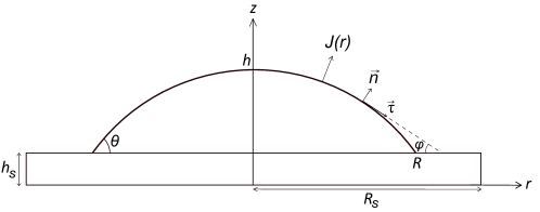
Figure 1: Sessile droplet on a solid substrate. The symmetry axis is $z$, the contact angle is $\theta$, and the local evaporation flux is $J(r)$.

The dynamics of vapor concentration $u(r,z)$ in the surrounding atmosphere is described by the diffusion equation

$$\dfrac{\partial u}{\partial t}=D\Delta u.$$ (1)

The boundary conditions are: $u=u_{s}$ on the drop surface, $u=0$ far away from the drop, $\partial u/\partial r=0$ and $\partial u/\partial z=0$ on the axes $r=0$ and $z=0$, correspondingly.

In the quasi-stationary approximation, the diffusion equation (1) can be replaced by the Laplace’s equation $\Delta u=0$. The approximation can be employed if the vapor concentration adjusts on time scales much less than the total drying time (i.e., $R^{2}/D$ is much smaller than $t_{f}\approx 0.2\rho Rh_{0}/(Du_{s})$), and if the Stefan flow can be neglected. The latter condition holds at room temperature and under atmospheric pressure, when the saturated vapor concentration is much smaller than the density of air (Fuchs, 1959). Within the quasi-stationary approximation and the spherical cap approximation, the analytical solution of the diffusion equation can be obtained which gives the inhomogeneous evaporation flux from the surface of the evaporating droplet (Deegan et al., 2000)

$$J_{s}(r)=\dfrac{Du_{s}}{R}\bigg{(}\dfrac{\sin{\theta}}{2}+\sqrt{2}(x(r)+\cos{\theta})^{3/2}\displaystyle\int_{0}^{\infty}\dfrac{\cosh{(\theta\tau)}}{\cosh{(\pi\tau)}}\tau\tanh((\pi-\theta)\tau)P_{-1/2+i\tau}(x(r))d\tau\bigg{)},$$ (2)

where

$$x(r)=\bigg{(}r^{2}\cos{\theta}/R^{2}+\sqrt{1-r^{2}\sin^{2}{\theta}/R^{2}}\bigg{)}\bigg{/}(1-r^{2}/R^{2})$$ (3)

and $P_{-1/2+i\tau}(x)$ is the Legendre polynomial. Expr. (2) can be conveniently approximated with high accuracy as (Deegan et al., 2000)

$$J_{s}(r)=J_{0}(\theta)(1-r^{2}/R^{2})^{-(1/2-\theta/\pi)},$$ (4)

where $J_{0}(\theta)$ can be determined by the following expressions (Hu and Larson, 2002):

$$J_{0}(\theta)/(1-\Lambda(\theta)) = J_{0}(\pi/2)(0.27\theta^{2}+1.3),$$ (5)

$$\Lambda(\theta) = 0.2239(\theta-\pi/4)^{2}+0.3619,$$ (6)

$$J_{0}(\pi/2) = Du_{s}/R.$$ (7)

Table 1: The notations and the parameter values used in the calculations.

				ethanol	1-butanol	1-hexanol
Drop	Initial temperature	$T_{0}$	K	$293.15$	$293.15$	$293.15$
parameters	Contact line radius	$R$	cm	$0.1$	$0.1$	$0.1$
Fluid	Density	$\rho$	g/cm3	$0.789$	$0.8098$	$0.8136$
parameters	Molar mass	$\mu$	g/mole	$46.07$	$74.122$	$102.17$
	Thermal conductivity	$k$	W/(cm$\cdot$ K)	$1.69\cdot 10^{-3}$	$1.54\cdot 10^{-3}$	$1.50\cdot 10^{-3}$
	Heat capacity	$c_{p}$	J/(mole K)	$112.3$	$177.2$	$240.4$
	Isochoric heat capacity	$c_{v}$	J/(g K)	$1.787$	$1.83$	$1.889$
	Thermal diffusivity	$\kappa$	cm2/s	$8.79\cdot 10^{-4}$	$7.95\cdot 10^{-4}$	$7.84\cdot 10^{-4}$
	Dynamic viscosity	$\eta$	g/(cm$\cdot$ s)	$1.074\cdot 10^{-2}$	$2.544\cdot 10^{-2}$	$4.578\cdot 10^{-2}$
	Surface tension	$\sigma$	g/s2	$21.97$	$24.93$	$25.81$
	$-\partial($surface tension$)/\partial T$	$-\sigma^{\prime}_{T}$	g/(s${}^{2}\cdot$ K)	$0.0832$	$0.0898$	$0.08$
	Latent heat of evap.	$L$	J/g	$918.6$	$706.27$	$603.0$
Substrate	Radius	$R_{S}$	cm	$0.125$	$0.125$	$0.125$
parameters	Thickness	$h_{S}$	cm	$0.02$	$0.02$	$0.02$
Vapor	Diffusion constant	$D$	cm2/s	$0.1181$	$0.0861$	$0.0621$
parameters	Saturated vapor density	$u_{s}$	g/cm3	$1.46\cdot 10^{-4}$	$2.76\cdot 10^{-5}$	$6.55\cdot 10^{-6}$

The above model of diffusion-limited evaporation assuming a constant vapor pressure along the interface is valid for a relatively small temperature gradients and/or only a minor slope in the vapor pressure chart. For a particular cases considered in the present study, the temperature difference along the interface is found to be of the order of $1$ K, and there is $\sim 5\%$ relative deviation of saturated vapor density as a result of the $1$ K change in temperature. Therefore, the above model can be employed to a first approximation.

It follows from (4) that the evaporating flux density is inhomogeneous along the surface and increases substantially on approach to the pinned contact line. A resulting inhomogeneous mass flow and corresponding heat transfer modify the temperature distribution along the droplet surface and, therefore, result in appearence of Marangoni forces associated with the temperature-dependent surface tension, which, in turn, generate convection inside the droplet.

The basic hydrodynamic equations inside the drop are the Navier-Stokes equations and the continuity equation for the incompressible fluid

$$\frac{\partial\textbf{{v}}}{\partial t}+(\textbf{{v}}\cdot\nabla)\textbf{{v}}+\frac{1}{\rho}\text{ grad }p=\nu\Delta\textbf{{v},}$$ (8)

$$\text{div {v}}=0.$$ (9)

Here $\Delta=\partial^{2}/\partial r^{2}+\partial/r\partial r+\partial^{2}/\partial z^{2}$, $\nu=\eta/\rho$ is kinematic viscosity, v is fluid velocity, $p$ is pressure. The boundary conditions are: $\left(v_{r}\right)_{r=0}=0$, $\left(\partial v_{z}/\partial r\right)_{r=0}=0$, $\textbf{v}=0$ at the solid–liquid interface (at $z=h_{S}$) and $\partial\sigma/\partial\tau=\eta(\partial v_{\tau}/\partial n-v_{\tau}\partial\varphi/\partial\tau)$ at the liquid–vapor interface (Barash et al., 2009).

The buoyancy force has been neglected in Eq.(8), because the buoyancy-induced convection is much weaker than Marangoni flow when $\rho gh^{2}\beta/(7\sigma^{\prime})\ll 1$, where $\beta$ is thermal expansion coefficient (Pearson, 1958). The latter condition holds for all the cases considered in the present study, including droplets of larger size in Sec. IV, where we always have $h<0.1$ cm.

The calculation of temperature distribution is carried out using the thermal conduction equation

$$\dfrac{\partial T}{\partial t}+\textbf{ v}\cdot\nabla T=\kappa\Delta T.$$ (10)

For relatively small and slowly evaporating droplets, when $Pe=\overline{v}R/\kappa\ll 1$, the convective heat transfer is much smaller than conductive heat transfer, and, hence, the velocity field does not influence the thermal conduction:

$$\dfrac{\partial T}{\partial t}=\kappa\Delta T.$$ (11)

This is the case, for example, for the droplet of 1-hexanol (see the parameters in Table 1). The thermal conduction inside the substrate is also described by (11).

We note that the transient time for heat transfer $t_{heat}=Rh_{0}/\kappa$, transient time for momentum transfer $t_{mom}=\rho Rh_{0}/\eta$ and transient time for vapor phase mass transfer $t_{mass}=u_{s}/\rho\cdot t_{f}$ are much smaller than the total drying time $t_{f}\approx 0.2\rho Rh_{0}/(Du_{s})$. This permits to describe the quasistationary stage of the evaporation process assuming a fixed geometric shape and disregarding the time derivatives in the heat conduction equation, Navier–Stokes equation and the diffusion equation (Larson, 2014).

Considering a fixed geometric shape, we also disregard the capillary flow, which is the coffee-stain outward flow (Deegan et al., 2000). This is justified in presence of a strong recirculating flow due to the Marangoni effect. Indeed, the velocity of the capillary flow is of the order of $R/t_{f}$ when the contact angle is not too small (see, e.g., the expressions in (Popov, 2005; Hu and Larson, 2005b; Kolegov and Barash, 2019)). Our numerical results confirm that the characteristic velocities of Marangoni flow are orders of magnitude larger than $R/t_{f}$.

The boundary conditions for the thermal conduction take the form $\partial T/\partial r=0$ for $r=0$; $T=T_{0}$ for $z=0$; $\partial T/\partial n=0$ at the substrate–gas interface, $k_{S}\partial T_{S}/\partial z=k_{L}\partial T_{L}/\partial z$ at the substrate–fluid interface, $\partial T/\partial n=-Q_{0}(r)/k$ at the drop surface. Here $T_{L}$ and $T_{S}$ correspond to the liquid and substrate temperature, $k_{L}$ and $k_{S}$ are thermal conductivities of liquid and substrate, respectively, $Q_{0}(r)=LJ_{s}(r)$ is the rate of heat loss per unit area of the upper free surface, n is a normal vector to the drop surface, $J_{s}(r)$ is determined by (4).

III Numerical simulation

We solve the thermal conduction equation and the Navier-Stokes equations by finite element method using computational fluid dynamics simulation package ANSYS Fluent designed for modeling the laminar flow, turbulence, heat transfer, and reactions for industrial applications.

The simulation includes several steps.

• Geometry and mesh generation

  We use two-dimensional geometry of the axially symmetrical surface according to Table 1. The surface curvature radius and the droplet height are equal to $R/\sin{\theta}$ and $R(1/\sin{\theta}-\cot{\theta})$, correspondingly. In ANSYS Fluent, the symmetry axis should be denoted as $x$-axis (as distinct from $z$-axis in Fig. 1). The next step is to divide the simulation region into small computational cells.

• Defining model and setting properties

  We choose the pressure-based solver type, 2D axisymmetric geometry, steady mode for time, viscous (laminar) flow and enable the calculation of energy in the model. We specify all physical properties of the fluid such as viscosity and density. The values are listed in Table 1 including the temperature derivative of the surface tension $\sigma^{\prime}_{T}=-\partial\sigma/\partial T$ which allows us to specify the properties of Marangoni stress.

• Setting boundary conditions and solution method

  The boundary conditions are set according to Section II. Some of the boundary conditions, such as at the symmetry axis, are automatically taken into account in ANSYS Fluent. The rate of heat loss $Q_{0}=LJ_{s}(r)$ is specified with user-defined function (UDF) written in the C programming language. The solution algorithm is SIMPLE (Semi-Implicit Method for Pressure Linked Equations). It uses a relationship between velocity and pressure corrections to enforce mass conservation and to obtain the pressure field. The algorithm is written in such a way that the continuity equation is automatically satisfied. See (Patankar, 2018) for detailed description of the SIMPLE algorithm.

• Post-processing

  We display the simulation results: velocity field, absolute values of velocity and temperature distribution, and analyse the vortex structure.

We note that our mesh contained at least 70000 cells for each contact angle. We used at least 20000 iterations to ensure that we obtained a steady state of the fluid flows in each case. Benchmark tests have been performed to ensure that a further increase of numbers of cells and iterations does not change the numerical results. Occasionly, when the obtained fluid flow structure was controversial, the numbers of cells and iterations were further increased to ensure the correctness of the results.

IV Phase diagrams for the number and orientation of vortices

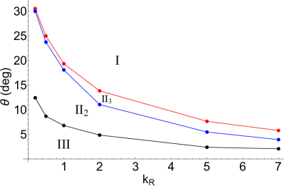
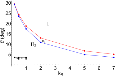
(a)                                                                  (b)

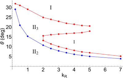
(c)

Figure 2: Results for $\theta$ vs $k_{R}=k_{S}/k_{L}$ for the droplet of (a) 1-hexanol, (b) 1-butanol and (c) ethanol, where the substrate temperature at the lower boundary is room temperature.

Consider the phase diagrams which represent the number and orientation of the vortices for quasistationary fluid flows in the droplet as functions of $k_{R}$ and $\theta$. Here, $k_{R}$ is ratio of substrate to fluid thermal conductivities and $\theta$ is the contact angle. The fluid flow fields have been numerically obtained and different phase diagram regions identified for several particular examples chosen (see Fig. 2). The notations I, II₂, II₃, III signify the phase diagram regions with single-vortex, two-vortex, three-vortex and reversed single-vortex regimes, respectively (Fig. 3).

We have determined the phase diagram regions via the numerically obtained fluid flow fields. The surface temperature distrubition usually follows the vortex structure in the droplet, although there are some exceptions to this rule due to the inertia of the fluid flow.

In our phase diagrams, the blue curve and black curve correspond to the change of sign of the tangential component of temperature gradient at the liquid–vapor interface, at the droplet apex and near the contact line, correspondingly. As shown in Ref. (Barash, 2015), with an increase of the substrate thickness, the subregion II₂ becomes dominating over II₃. Further increase of the substrate thickness results in shifting the regions I and II to larger contact angles. The blue curve is situated below the black curve at small values of $h_{R}=h_{S}/R$, while for $h_{R}\gtrsim 0.05$ the blue curve is above the black curve (Barash, 2015). The phase diagrams in Fig. 2 correspond to the latter case.

For $h_{R}\gtrsim 0.05$, the transition between the regions III and II₂ corresponds to the change of sign of the tangential component of the temperature gradient at the liquid–vapor interface near the contact line. The transition between the regions II₂ and II₃ corresponds in this case to the change of sign of the tangential component of the temperature gradient at the liquid–vapor interface at the droplet apex. The transition between the regions I and II₃ corresponds to the change between a nonmonotonic dependence of surface temperature on $r$ and a monotonically increasing surface temperature with $r$.

The main features of the phase diagram can be qualitatively understood as a result of matching the heat transfer across the solid–liquid interface and the vaporization heat through the liquid–vapor interface (see details in (Zhang et al., 2014; Barash, 2015)). As a result of the matching and competition of these two effects, vortex structures are formed which depend on the values of $k_{R}$ and $\theta$.

Consider now the volatility effect on the phase diagram. Fig. 2 shows the phase diagrams obtained for the three droplets of different liquids, where the parameters of the droplets are listed in Table 1. Since the saturated vapor density of 1-hexanol, 1-butanol and ethanol differ by orders of magnitude as seen in Table 1, the evaporation rates (volatilities) of these liquids described by Eqs.(4)-(7) also significantly differ.

As seen in Fig. 2, with an increase of the fluid volatility, the subregion III disappears; the subregion II₂ increases at the expense of the subregion III; the subregion II₃ becomes larger at the expense of the subregion I; the subregion I diminishes for small values of $k_{R}$ and becomes more complex for highly volatile liquids.

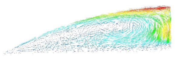
(a)

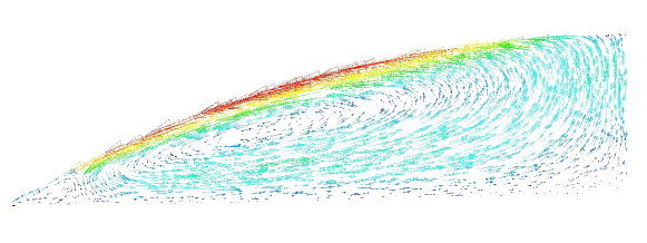
(b)

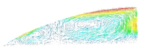
(c)

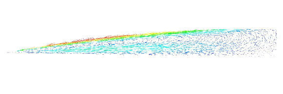
(d)

Figure 3: Examples of vector field plots of velocity obtained for (a) single-vortex, (b) two-vortex, (c) three-vortex and (d) reversed single vortex regimes.

$\theta$	$R$(mm)	$R_{s}$(mm)	$h_{s}$(mm)	Bond number	$k_{R}=0.2$	$k_{R}=0.5$	$k_{R}=1$	$k_{R}=2$	$k_{R}=5$	$k_{R}=7$
$32^{\circ}$	1	1.25	0.2	0.084	single	single	single	single	single	single
$30^{\circ}$	1	1.25	0.2	0.083	two	single	single	single	single	single
$30^{\circ}$	2	3	0.3	0.313	two	single	single	single	single	single
$30^{\circ}$	3	5	0.5	0.641	two	two	single	single	single	single
$30^{\circ}$	4	6	0.75	1.021	two	two	two	single	single	single
$30^{\circ}$	5	8	1	1.412	two	two	two	two	single	single
$30^{\circ}$	6	9	1	1.794	two	two	two	two	two	single
$30^{\circ}$	7	10	1	2.157	two	two	two	two	two	two
$30^{\circ}$	9	12	2	2.834	two	two	two	two	two	two

Table 2: Numbers of vortices in the droplets of 1-butanol of different size.

Domination of the evaporative cooling as compared to the heat flow at the substrate-liquid interface leads to the reversed single-vortex regime for small values of $k_{R}$ and at small contact angles, for weakly volatile liquids Barash (2015). For highly volatile liquids, however, the cooling of the droplet bulk is a faster process resulting in a larger temperature difference between the droplet bulk and the substrate, which, in turn, leads to increasing the heat flow at the substrate-liquid interface close to the contact line even for moderately low values of $k_{R}$. This is in accordance with the disappearance of the subregion III for highly volatile liquids as observed in Fig. 2.

Increasing the fluid volatility results in larger chances of domination of the vaporization heat for relatively large contact angles. This is in accordance with the shift of the subregion I at relatively small values of $k_{R}$ to larger contact angles. Understanding of the complex structure of subregion I shown in Fig. 2(c) for relatively large values of $k_{R}$ requires an additional study.

Consider now the effect of droplet size on the phase diagram. The fluid flow structure has been calculated for droplet size exceeding that in Table 1. The droplet shape becomes nonspherical when $B_{o}\gtrsim 1$, where $B_{o}=\rho ghR/(2\sigma\sin\theta)$ is Bond number for the sessile droplet, where $h$ is the droplet height. In this case, we obtained the droplet shape taking into account influence of gravity. Nonspherical droplet free surface was obtained with the Runge-Kutta numerical method using the approach described in (Barash et al., 2009).

We find that the phase diagrams for droplets of larger size do not contain the subregions I and II₃. Table 2 shows numbers of vortices in the droplet of 1-butanol of different size for $\theta\approx 30^{\circ}$. It demonstrates that droplets of capillary size contain a single-vortex for $\theta\approx 30^{\circ}$, while larger droplets contain two vortices in this case. Although the existence of subregion I depends on $k_{R}$, the subregion I disappears with gradually increasing the droplet radius $R$ for each $k_{R}$, as shown in Table 2.

The absence of subregion I for large droplets can be understood as follows. In order for the subregion I to occur, the heat transfer through the solid-liquid interface should dominate compared to the vaporization heat. For droplets of larger size, the former heat flow becomes relatively weak for the regions far away from the substrate. Therefore, the vaporization heat dominates there, and the vortex splits into two vortices.

V Conclusion

We have performed numerical simulations of the fluid flow structure in evaporating sessile droplets depending on thermal conductivities of liquid and substrate, liquid volatility, contact angle and droplet size, and we have analyzed the corresponding phase diagrams in the $k_{R}$–$\theta$ plane.

We find that with an increase of the fluid volatility, the subregion I becomes more complex and the subregion III disappears; the subregion II₂ increases at the expense of the subregion III; the subregion II₃ becomes larger at the expense of the subregion I. Also, we have shown that the phase diagrams for droplets of larger size do not contain the subregions I and II₃.

The results may provide a better understanding of the Marangoni effect of drying droplets and may be useful for preparing the fluid flow vortex structure in a controlled manner by selecting substrates and liquids with appropriate properties. Also, the results may potentially be useful to better understand evaporative deposition patterns and evaporative self-assembly of nanostructures.

References

- Brutin and Starov (2018) D Brutin and V Starov, “Recent advances in droplet wetting and evaporation,” Chem. Soc. Rev. 47, 558–585 (2018).
- Erbil (2012) H Yildirim Erbil, “Evaporation of pure liquid sessile and spherical suspended drops: A review,” Adv. Colloid Interface Sci. 170, 67–86 (2012).
- Larson (2014) Ronald G Larson, “Transport and deposition patterns in drying sessile droplets,” AIChE J. 60, 1538–1571 (2014).
- Thiele (2014) Uwe Thiele, “Patterned deposition at moving contact lines,” Adv. Colloid Interface Sci. 206, 399–413 (2014).
- Zang et al. (2019) Duyang Zang, Sujata Tarafdar, Yuri Yu. Tarasevich, Moutushi Dutta Choudhury, and Tapati Dutta, “Evaporation of a droplet: From physics to applications,” Phys. Rep. 804, 1–56 (2019).
- Harris et al. (2007) Daniel J. Harris, Hua Hu, Jacinta C. Conrad, and Jennifer A. Lewis, “Patterning colloidal films via evaporative lithography,” Phys. Rev. Lett. 98, 148301 (2007).
- Kolegov and Barash (2020) K. S. Kolegov and L. Yu. Barash, “Applying droplets and films in evaporative lithography,” Preprint 2005.07148 (2020).
- Bigioni et al. (2006) Terry P Bigioni, Xiao-Min Lin, Toan T Nguyen, Eric I Corwin, Thomas A Witten, and Heinrich M Jaeger, “Kinetically driven self assembly of highly ordered nanoparticle monolayers,” Nat. Mater. 5, 265 (2006).
- Savino and Fico (2004) R. Savino and S. Fico, “Transient marangoni convection in hanging evaporating drops,” Phys. Fluids 16, 3738–3754 (2004).
- Kang et al. (2004) Kwan Hyoung Kang, Sang Joon Lee, Choung Mook Lee, and In Seok Kang, “Quantitative visualization of flow inside an evaporating droplet using the ray tracing method,” Meas. Sci. Technol. 15, 1104–1112 (2004).
- Hu and Larson (2006) Hua Hu and Ronald G. Larson, “Marangoni effect reverses coffee-ring depositions,” J. Phys. Chem. B 110, 7090–7094 (2006).
- Ristenpart et al. (2007) W. D. Ristenpart, P. G. Kim, C. Domingues, J. Wan, and H. A. Stone, “Influence of substrate conductivity on circulation reversal in evaporating drops,” Phys. Rev. Lett. 99, 234502 (2007).
- Xu et al. (2010) Xuefeng Xu, Jianbin Luo, and Dan Guo, “Criterion for reversal of thermal marangoni flow in drying drops,” Langmuir 26, 1918–1922 (2010).
- Hu and Larson (2005a) Hua Hu and Ronald G. Larson, “Analysis of the effects of marangoni stresses on the microflow in an evaporating sessile droplet,” Langmuir 21, 3972–3980 (2005a).
- Patil et al. (2016) Nagesh D. Patil, Prathamesh G. Bange, Rajneesh Bhardwaj, and Atul Sharma, “Effects of substrate heating and wettability on evaporation dynamics and deposition patterns for a sessile water droplet containing colloidal particles,” Langmuir 32, 11958–11972 (2016).
- Girard et al. (2010) Fabien Girard, Mickaël Antoni, and Khellil Sefiane, “Infrared thermography investigation of an evaporating sessile water droplet on heated substrates,” Langmuir 26, 4576–4580 (2010).
- Sobac and Brutin (2012) B. Sobac and D. Brutin, “Thermal effects of the substrate on water droplet evaporation,” Phys. Rev. E 86, 021602 (2012).
- Zhang et al. (2014) Kai Zhang, Liran Ma, Xuefeng Xu, Jianbin Luo, and Dan Guo, “Temperature distribution along the surface of evaporating droplets,” Phys. Rev. E 89, 032404 (2014).
- Barash (2015) L.Yu. Barash, “Dependence of fluid flows in an evaporating sessile droplet on the characteristics of the substrate,” Int. J. Heat Mass Transfer 84, 419–426 (2015).
- Sefiane et al. (2008) K. Sefiane, J. R. Moffat, O. K. Matar, and R. V. Craster, “Self-excited hydrothermal waves in evaporating sessile drops,” Appl. Phys. Lett. 93, 074103 (2008).
- Carle et al. (2012) F. Carle, B. Sobac, and D. Brutin, “Hydrothermal waves on ethanol droplets evaporating under terrestrial and reduced gravity levels,” J. Fluid Mech. 712, 614–623 (2012).
- Zhu et al. (2019) Ji-Long Zhu, Wan-Yuan Shi, and Lin Feng, “Bénard-marangoni instability in sessile droplet evaporating at constant contact angle mode on heated substrate,” Int. J. Heat Mass Transfer 134, 784–795 (2019).
- Fuchs (1959) Nikolai Albertovich Fuchs, Evaporation and droplet growth in gaseous media (Pergamon Press, Oxford, 1959).
- Deegan et al. (2000) Robert D. Deegan, Olgica Bakajin, Todd F. Dupont, Greg Huber, Sidney R. Nagel, and Thomas A. Witten, “Contact line deposits in an evaporating drop,” Phys. Rev. E 62, 756–765 (2000).
- Hu and Larson (2002) Hua Hu and Ronald G. Larson, “Evaporation of a sessile droplet on a substrate,” J. Phys. Chem. B 106, 1334–1344 (2002).
- Barash et al. (2009) L. Yu. Barash, T. P. Bigioni, V. M. Vinokur, and L. N. Shchur, “Evaporation and fluid dynamics of a sessile drop of capillary size,” Phys. Rev. E 79, 046301 (2009).
- Pearson (1958) J. R. A. Pearson, “On convection cells induced by surface tension,” J. Fluid Mech. 4, 489–500 (1958).
- Popov (2005) Yuri O. Popov, “Evaporative deposition patterns: Spatial dimensions of the deposit,” Phys. Rev. E 71, 036313 (2005).
- Hu and Larson (2005b) H. Hu and R. G. Larson, “Analysis of the microfluid flow in an evaporating sessile droplet,” Langmuir 21, 3963–3971 (2005b).
- Kolegov and Barash (2019) K. S. Kolegov and L. Yu. Barash, “Joint effect of advection, diffusion, and capillary attraction on the spatial structure of particle depositions from evaporating droplets,” Phys. Rev. E 100, 033304 (2019).
- Patankar (2018) Suhas V Patankar, Numerical heat transfer and fluid flow (CRC Press, 2018).