Semantic Labeling of Large-Area Geographic Regions Using Multi-View and Multi-Date Satellite Images and Noisy OSM Training Labels

Abstract

We present a novel multi-view training framework and CNN architecture for combining information from multiple overlapping satellite images and noisy training labels derived from OpenStreetMap (OSM) to semantically label buildings and roads across large geographic regions (100 km²). Our approach to multi-view semantic segmentation yields a 4-7% improvement in the per-class IoU scores compared to the traditional approaches that use the views independently of one another. A unique (and, perhaps, surprising) property of our system is that modifications that are added to the tail-end of the CNN for learning from the multi-view data can be discarded at the time of inference with a relatively small penalty in the overall performance. This implies that the benefits of training using multiple views are absorbed by all the layers of the network. Additionally, our approach only adds a small overhead in terms of the GPU-memory consumption even when training with as many as 32 views per scene. The system we present is end-to-end automated, which facilitates comparing the classifiers trained directly on true orthophotos vis-a-vis first training them on the off-nadir images and subsequently translating the predicted labels to geographical coordinates. With no human supervision, our IoU scores for the buildings and roads classes are 0.8 and 0.64 respectively which are better than state-of-the-art approaches that use OSM labels and that are not completely automated.

I Introduction

In this work, we are interested in answering the following question – Is there an optimal way to combine multi-view and multi-date satellite images, and noisy training labels derived from OpenStreetMap (OSM) [1] for the task of semantically labeling buildings and roads on the ground over large geographic regions (100 km²)? Note that labeling points on the ground is more challenging than labeling pixels in images because the former requires that we first map each point on the ground to the correct pixel in each image. This is only possible if (1) the multi-date and multi-view images are not only aligned with one another but are also aligned well in an absolute sense to the real world; and (2) if we have accurate knowledge of the heights of the points on the ground.

Before summarizing our main contributions, to give the reader a glimpse of the power of the approach presented in this study, we show some sample results in Fig. 1.

Single-View Training (Baseline)
Multi-View Training (Proposed Approach)

Figure 1: To illustrate the power of our approach, the buildings in the bottom row were extracted by our approach based on multi-view training for semantic labeling. Compare with the top row where the training is based on single-views. Building points are marked in translucent blue.

Towards answering the aforementioned question, we put forth the following contributions:

1. We present a novel multi-view training paradigm that yields improvements in the range 4-7% in the per-class IoU (Intersection over Union) metric. Our evaluation directly demonstrates that updating the weights of the convolutional neural network (CNN) by simultaneously learning from multiple views of the same scene can help alleviate the burden of noisy training labels.

2. We present a direct comparison between training classifiers on 8-band true orthophoto images vis-a-vis training them on the original off-nadir images captured by the satellites. The fact that we use OSM training labels poses challenges for the latter approach, as it necessitates the need to transform labels from geographic coordinates into the off-nadir image-pixel coordinates. Such a transformation requires that we have knowledge of the heights of the points. The comparison presented in this study is unlike most published work in the literature that use pre-orthorectified single-view images. Additionally, we have released our software for creating true orthophotos, for public use. Interested researchers can download this software from the link at [2].

3. In order to make the above comparison possible, we present a true end-to-end automated framework that aligns large multi-view, multi-date images (each containing about $43008\times 38000$ pixels), constructs a high-resolution accurate Digital Surface Model (DSM) over a 100 km² area (which is needed for establishing correspondences between the pixels in the off-nadir images and points on the ground), and learns from noisy OSM labels without any additional human supervision.

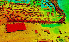
(a)

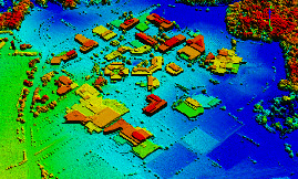
(b)

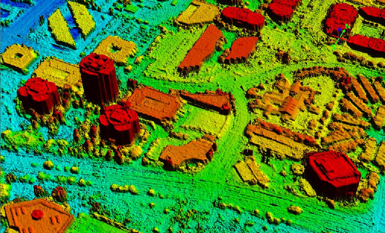
(c)

(d)

Figure 2: We have uploaded as Supporting Material the flyby videos and the images of the DSMs for two large areas, a 120 km² area from Ohio and a 62 km² area from California. The flyby videos can also be viewed at the link at [3]. The top two images depict two small sections from the Ohio DSM, and the bottom two images depict two small sections from the California DSM. The DSM depictions have been colored according to the elevation values within the boundaries of each section.

For our study, we use WorldView-3 (WV3) [4] images collected over two regions in Ohio and California, USA. We use 32 images for each region. The images were collected across a span of 2 years under varying conditions. Automatic alignment and DSM construction are carried out for both regions. Smaller sections of these DSMs are shown in Fig. 2.

The rest of this manuscript is organized as follows. In Section II, we briefly review relevant literature. Section III provides details on aligning images, creating large-area DSMs, and deriving training labels from OSM. Section IV presents different approaches for training and inference using CNNs. Section V discusses a strategy for using training labels derived from OSM to label off-nadir images. Experimental evaluation is described in Section VI. Concluding remarks are presented in Section VII.

II Literature Review

State-of-the-art approaches that demonstrate the use of labels derived from OSM for finding roads and/or buildings in overhead images include the studies described in [5], [6], [7], [8], [9], [10], [11], [12], [13], [14], [15], [16], [17], [18], [19], [20] and [21]. Many of these approaches use some category of neural networks as part of their machine-learning frameworks. For instance, while the study described in [5] uses a CNN backbone to extract keypoints that are subsequently input to a recurrent neural network (RNN) to extract building polygons and road networks, the approach presented in [6] constructs a road network in an iterative fashion by using a CNN to detect the next road segment given the previously extracted road network. The work discussed in [10] builds upon the approach in [6] by using a generative adversarial network (GAN) [22] to further refine the outputs. In addition, the recent contributions in [23], [24], [25], [26], [27], [28] and [29] use datasets with precise training labels for semantic labeling of overhead imagery. All these approaches use single-view images that are usually pre-orthorectified.

Some examples of popular datasets for semantic labeling of overhead imagery with manually-generated and/or manually-corrected training labels can be found in [30], [31], [32], [33], [34], [35], [36], [37], [38] and [39]. The dataset presented in [32] provides satellite images, airborne LiDAR, and building labels (derived from LiDAR) that are manually corrected. The DeepGlobe dataset [30] provides satellite images and precise labels (annotated by experts) for land cover classification and road and building detection. The study described in [34] combines multi-view satellite imagery and large-area DSMs (obtained from commercial vendors) [33] with building labels that are initialized using LiDAR from the HSIP 133 cities data set [40]. The IEEE GRSS Data Fusion Contest dataset [35], [36] provides true ortho images, LiDAR and hyperspectral data along with precise groundtruth labels for 17 local climate zones. A summary of the top-performing algorithms on this dataset can be found in [41].

We will restrict our discussion of prior contributions that use information from multiple views to CNN-based approaches. Variants of multi-view CNNs have been proposed primarily for segmentation of image-sequences and video frames, and for applications such as 3D shape recognition/segmentation and 3D pose estimation. State-of-the-art examples include the approaches described in [42], [43], [44], [45], [46], [47], [48], [49], [50], [51], [52], [53] and [54]. These contributions share one or more of the following attributes: (1) They synthetically generate multiple views by either projecting 3D data into different planes, or by viewing the same image at multiple scales; (2) They extract features from multiple views, concatenate/pool such features and/or enforce consistency checks between the features; (3) They use only a few views (of the order of 5 or less). For instance, while the study described in [42] improves semantic segmentation of RGB-D video sequences by enforcing consistency checks after projecting the sequences into a reference view at training time, the approach presented in [44] estimates 3D hand pose by first projecting the input point clouds onto three planes, subsequently training CNNs for each plane and then fusing the output predictions.

With respect to the field of remote-sensing, multi-date satellite images have been used for applications such as change detection. For instance, the study described in [55] demonstrates unsupervised change-detection between a single pair of images with deep features extracted using a cycle-consistent GAN [56]. However, there do not exist many studies that use CNNs for labeling of multi-view and multi-date satellite images. A relevant contribution is the one described in [57] that won the 2019 IEEE GRSS Data Fusion Contest for Multi-View Semantic Stereo [58]. The work in [59] also uses off-nadir WV3 images for semantic labeling. Both these approaches still treat the different views of the same scene on the ground independently during training. To the best of our knowledge, there has not existed prior to our work reported here a true multi-view approach for semantic segmentation using satellite images.

We also include a brief review of the literature related to constructing DSMs from satellite images. Fully automated approaches for constructing DSMs from satellite images have been discussed in [60], [61], [62], [63], [64], [65] and [66]. While the studies described in [61], [62] and [64] process pairs of images to construct multiple pairwise point clouds that are subsequently fused to construct a dense DSM, the contribution in [63] compares such approaches with an alternative approach that divides the 3D scene into voxels, projects each voxel into all the images and subsequently reasons about the probability of occupancy of each voxel using the corresponding pixel features from all the images. In all of these contributions, the DSMs that are constructed cover relatively small areas. The large-area DSM contribution in [67] is based on a small number of in-track images that are typically captured seconds or minutes apart by the Pléiades satellite. In addition to the aforementioned contributions, the study in [68] provides a dataset containing stereo-rectified images and the associated groundtruth disparity maps for different world regions, that can be used for benchmarking stereo-matching algorithms.

III A Framework for Large-Area Image Alignment, DSM Creation, and Generating Training Samples from OSM

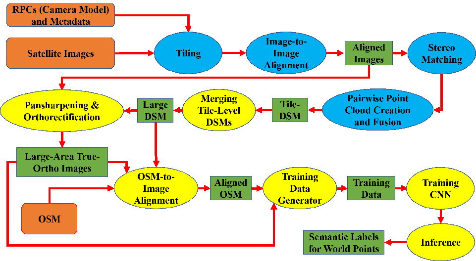
Figure 3: Overview of our framework. The three inputs are shown in orange-colored boxes. All outputs produced by the system are shown in green-colored boxes. The modules in blue-colored ellipses operate on a tile-wise basis.

As stated in the Introduction section, our goal is to generate accurate semantic labels for the points on the ground (as opposed to the pixels in the images). Solving this problem requires correcting the positioning errors in the satellite cameras and estimating accurate elevation information for each point on the ground — since only then we can accurately establish the relationship between the pixels in the images and the points on the ground. This will also enable us to establish correspondences between the pixels of the multiple views of the same scene.

Therefore, an important intermediate step in our processing chain is the calculation of the DSM. To the best of our knowledge, there is no public contribution that discusses a complete framework for automatic alignment and creation of large-area DSMs over a 100 km² region using satellite images taken as far apart as 2 years. Because of the role played by high-quality large-area DSMs in our framework, we have highlighted this part of the framework in the Introduction and shown some sample results in Fig. 2.

An overview of the overall framework presented in this study is shown in Fig. 3. The system has three inputs that are shown by the orange colored boxes: (1) panchromatic and 8-band multispectral satellite images; (2) the metadata associated with the images; and (3) the OSM vectors. After the CNN is trained in the manner described in the rest of this manuscript, the framework directly outputs semantic labels for the world points. In the rest of this section, we will briefly describe the major components of the framework, apart from the machine-learning component. These components are described in greater detail in the Appendices.

The notion of a tile is used only for aligning the images and for constructing a DSM. For the CNN-based machine-learning part of the system, we work directly with the whole images and with the OSM for the entire area of interest. Tiling is made necessary by the following two considerations: (1) The alignment correction parameters for a full satellite image cannot be assumed to be the same over the entire image; (2) The computational requirements for image-to-image alignment and DSM construction become too onerous for full-sized images. We have included evidence for the need for tiling in Appendix A-B. On a related note, the study reported in [69] describes an approach that divides a large region into smaller chips for the purpose of land cover clustering. After tiling, the images are aligned with bundle-adjustment algorithms, which is a standard practice for satellite images. Alignment in this context means calculating corrections for the rational polynomial coefficients (RPCs) of each image.

A DSM is constructed from the disparity map generated by the hierarchical tSGM algorithm [70]. Stereo matching is only applied to those pairs that pass certain prespecified criteria with respect to differences in the view angles, sun angles, time of acquisition, etc., subject to the maximization of the azimuth angle coverage. The disparity maps and corrected RPCs are used to construct pairwise point clouds. Since the images have already been aligned, the corresponding point clouds are also aligned and can be fused without any further 3D alignment. Tile-level DSMs are merged into a large-area DSM.

The training data is generated by using an $F\times F$ window to randomly sample the images after they have been pansharpened and orthorectified using the DSM. We refer to such an $F\times F$ window on the ground as a ground-window. The parameter $F$ is empirically set to 572 in our experiments. Subsequently, the OSM vectors are converted to raster format with the same resolution as in the orthorectified images. Thus there is a label for each geographic point in the orthorectified images. The OSM roads are thickened to have a constant width of 8m. Since the images are aligned with sub-pixel accuracy and are orthorectified, the training samples from the multiple images that view the same ground-window correspond to one another on a point-by-point basis, thereby giving us multi-view training data.

IV Multi-View Training and Inference

IV-A Motivation for our Proposed Approach

Our multi-view training framework is motivated by the following factors:

With newer and better single-view CNNs being designed so frequently, it would be convenient if the multi-view fusion module could be designed as an add-on to an existing pretrained architecture. This would make it easy to absorb the latest improvements in the single-view architectures directly into the multi-view fusion framework. We won’t have to rethink the feature concatenation for each new single-view CNN architecture. Additionally, we want to efficiently train the single-view weights in parallel across multiple GPUs and carry out fusion on a single GPU.

The satellite images could have been collected years apart under different illumination and atmospheric conditions. Thus, our task is very different from traditional multi-view approaches that work with 3D shapes or images captured by moving a (handheld) camera around the same scene.

The number of views covering a ground-window can vary between 1 to all available images (32 in our case). This causes practical challenges in backpropagating gradients when using CNNs that assume the availability of a fixed number of views for concatenating features. At the same time, we do not want to exclude windows that are covered by less than a specified number of views. Our goal is to use all available training data and all available views for every ground-window.

IV-B Multi-View Fusion Module

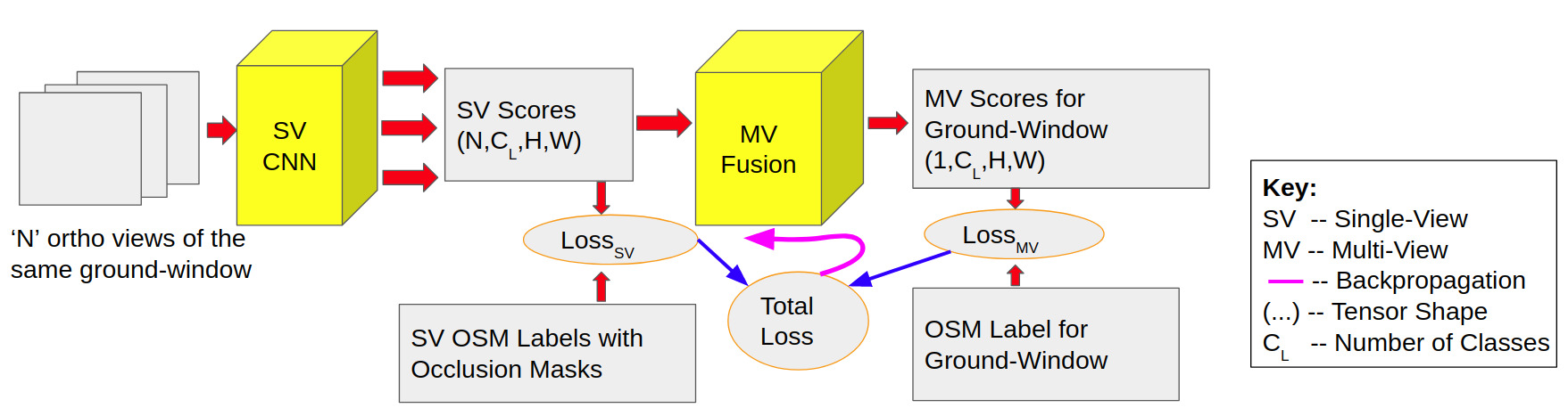
Figure 4: Overview of Multi-View Training

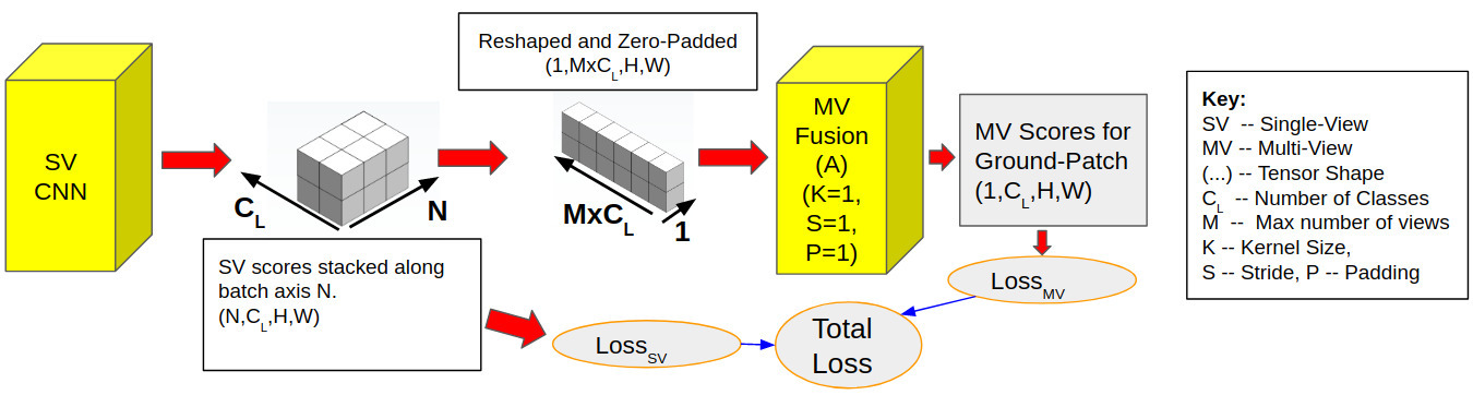
(a)

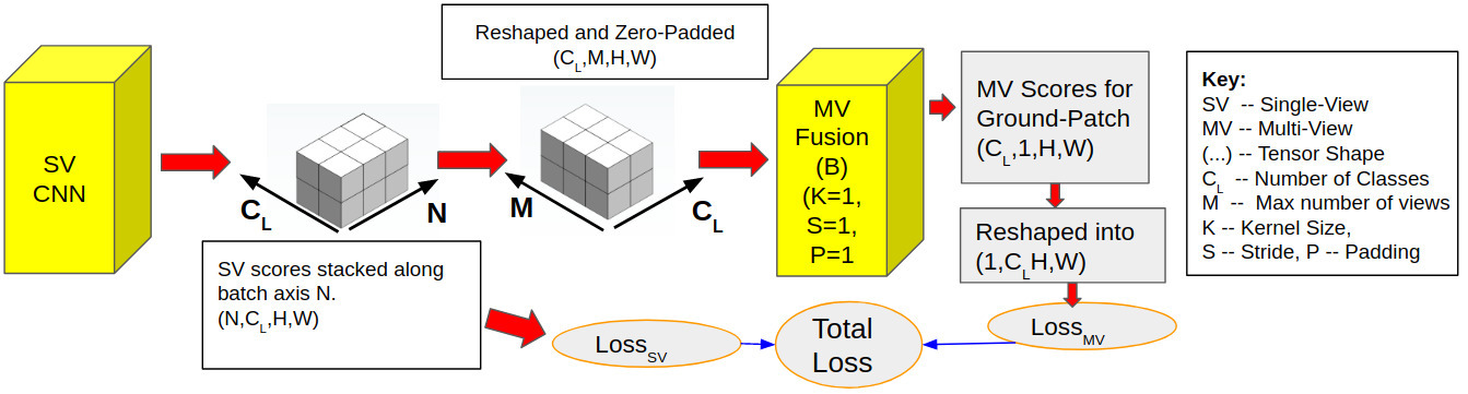
(b)

Figure 5: Two choices for Multi-View Fusion. At top is MV-A in which the weights of the MV Fusion layer are different for each channel of each view. At bottom is MV-B where the weights of the MV Fusion layer are shared by all the channels of a view.

Fig. 4 shows an overview of our multi-view training framework where we propose that the multi-view information be aggregated at the predictions stage. In this sense, our approach is related to the strategies discussed in [49] and [54]. While the contribution in [49] considers the “RGB” and the depth channel of the same RGB-D image as two “views” (which is a much simpler case), the 3D shape segmentation approach in [54] synthetically generates multiple-views of the same 3D object. In contrast, the significantly more complex nature of our data makes our problem very different from these tasks.

The multi-view fusion module shown in Fig. 4 can be added to any existing/pretrained single-view CNN. We experimented with different choices for this module and present two that gave good performance yields. These are shown in Fig. 5 and we denote them as MV-A (Multi-View-A) and MV-B(Multi-View-B) respectively. Both MV-A and MV-B consist of a single block of weights with kernel size, stride and padding set to 1.

In the following discussion, $V$ denotes a subset of views for a single ground-window. $N$ is the number of views in $V$. $H$ and $W$ are the height and width of a single view respectively. $M$ is the maximum number of possible views for a ground-window. $C_{L}$ is the number of target classes.

As shown in Fig. 4, the Single-View (SV) CNN outputs a tensor of shape $(C_{L},H,W)$ for each of N views which are concatenated along the batch axis to yield a tensor of shape $(N,C_{L},H,W)$, which we denote as $T^{N}_{MV}$. This tensor is then inserted into a larger tensor which we denote as $T_{MV}$. Each view has a fixed index in $T_{MV}$. Missing views are filled with zeros. The difference between MV-A and MV-B can now be explained as follows.

In this case, $T^{N}_{MV}$ is reshaped into a tensor of shape $(1,N\times C_{L},H,W)$. It is then inserted into $T_{MV}$ which is of shape $(1,M\times C_{L},H,W)$. $T_{MV}$ is then input to the MV-A module which subsequently outputs a tensor of shape $(1,C_{L},H,W)$. MV-A thus contains a total of $M\times C_{L}$ trainable weights, one for each channel of each view.

In this case, $T^{N}_{MV}$ is first reshaped into a tensor of shape $(C_{L},N,H,W)$. It is then inserted into $T_{MV}$ which is of shape $(C_{L},M,H,W)$. $T_{MV}$ is then input to the MV-B module which subsequently outputs a tensor of shape $(C_{L},1,H,W)$. MV-B thus contains a total of $M$ trainable weights, one for each view. The first and second axis of this tensor are swapped to yield a tensor of shape $(1,C_{L},H,W)$ which is then used to calculate the loss.

IV-C Multi-View Loss Function

The total loss is defined as

$$L=\alpha\cdot L_{SV}+\beta\cdot L_{MV}$$ (1)

where $L_{SV}$ represents the single-view loss, $L_{MV}$ represents the multi-view loss and $\alpha$ and $\beta$ are scalars used to weight the two loss functions. The single-view loss is calculated as follows.

$$L_{SV}=\frac{1}{N}\sum_{i=1}^{N}\text{CE${}_{i}(G_{i},T_{i})$}$$ (2)

where CE_i is the pointwise cross-entropy loss for the $i^{th}$ view, $N$ is the number of views in a subset $V$ of views that cover a single ground-window and $T_{i}$ is the output tensor of the SV CNN for the $i^{th}$ view. To calculate CE_i, we mask the OSM labels for the ground-window with the occlusion mask of the $i^{th}$ view. This masked ground-truth is denoted by $G_{i}$ in the equation above. Note that this mask is implicitly computed during the process of true orthorectification. The gradients of $L_{SV}$ are not backpropagated at these masked points. What this means is that for each individual view, $L_{SV}$ only focuses on portions of the ground-window that are visible in that view.

The pointwise cross-entropy loss between two probability distributions $A$ and $B$, each defined over $C_{L}$ classes, is calculated as follows.

$$\text{CE}(A,B)=-\sum_{p}\sum^{C_{L}}_{j=1}A(p,j)\cdot log(B(p,j))$$ (3)

where $p$ refers to a single point. $A(p,j)$ is the probability that point $p$ belongs to class $j$ as defined by $A$. $B(p,j)$ is the probability that point $p$ belongs to class $j$ as defined by $B$.

The multi-view loss is calculated as follows.

$$L_{MV}=\text{CE}(G,P_{MV})$$ (4)

where CE$(G,P_{MV})$ is the pointwise cross-entropy loss for the ground-window. This is calculated using the unmasked OSM label $G$ and the output $P_{MV}$ of the MV Fusion module. $P_{MV}$ can be viewed as a final probability distribution that is estimated by fusing the individual probability distributions that are output by the SV CNN for each of the $N$ views. We can denote $P_{MV}$ as a function $f(T_{1},T_{2},...,T_{N})$ where $f$ depends upon the architecture of the MV Fusion module. Note that $f$ is differentiable. Thus, Eq. 4 can be rewritten as

$$L_{MV}=\text{CE}(G,f(T_{1},T_{2},...,T_{N}))$$ (5)

Substituting the expression for the CE loss from Eq. 3 into Eq. 5, we get the following expression for $L_{MV}$.

$$L_{MV}=-\sum_{p}\sum^{C_{L}}_{j=1}G(p,j)\cdot log(f(T_{1},T_{2},...,T_{N})(p,j))$$ (6)

Note that $L_{MV}$ is not linearly separable over the views in V. In other words, unlike $L_{SV}$, we cannot separate it into a sum of losses for each view. Thus, $L_{MV}$ captures the predictions of the network in an ensemble sense over multiple views covering a ground-window. When backpropagating the gradients of $L$, the gradients from $L_{MV}$ are influenced by the relative differences between the predictions for each view, and this in turn translates into better weight-updates. Moreover, by using $L_{MV}$, the network is shown labels for all portions of the ground including those that are missing in some views of $V$. This enables the network to make better decisions about occluded regions using multiple views.

IV-D Strategies for Multi-View Training and Inference

IV-D1 Approaches for Data-Loading

The term “data-loading” refers to how the data samples are grouped into batches and input to the CNN. We use two different data-loading approaches.

This is a conventional data-loading strategy where a single training batch can contain views of different ground-windows. The batch size is constant and only depends on the available GPU memory. SV DATALOAD uses all the available data.

Under this strategy, a training batch consists solely of views that cover the same ground-window. The number of such views can vary from window to window. However, due to memory constraints, we cannot load all 32 views onto the GPUs simultaneously. As a work around, we use the following approach. Let $|Q|$ denote a pre-specified number of views that can fit into the GPU memory, $R$ denote the set of available views for a ground-window and $|R|$ denote the total number of views in $R$. If $|R|<|Q|$, we skip loading this ground-window. If $|R|>|Q|$, we randomly split $R$ into a collection of overlapping subsets $\{Q_{j}\}$, such that each $Q_{j}$ has $|Q|$ views and $\cup Q_{j}=R$ where $\cup$ denotes the union operator. The tensor $T_{MV}$ that is input to the MV Fusion module is reset to zero before inputting each $Q_{j}$ to the CNN. Note that this random split has the added advantage that the CNN sees a different collection of views for the same ground-window in different epochs, which should help it to learn better.

The design of MV DATALOAD is motivated by our observation that if we allow the batch size to change significantly for every ground-window (based on the corresponding number of available views), it significantly slows down the rate of convergence. Therefore, we exclude ground-windows with less than $|Q|$ views, and for the remaining windows we make sure that every subset $Q_{j}$ has $|Q|$ views. This enforces a constant batch size of $|Q|$, resulting in faster convergence.

IV-D2 Training Strategies

We use the following different strategies to train the CNNs.

Single-View Training (SV TRAIN): In this strategy, the SV CNN is trained independently of the MV Fusion module. We apply the SV DATALOAD approach to use all available data. One can also interpret this as setting $\beta=0$ in Eq. 1 and freezing the weights of the MV Fusion module.

We now define three different multi-view training strategies as follows.

We first train the SV CNN using SV TRAIN. Subsequently, we use MV DATALOAD to only train the MV Fusion module by setting $\alpha=0$ in Eq. 1, and by freezing the weights of the SV CNN. Hence, $L_{MV}$ only affects the weights of the MV Fusion module and does not affect the SV CNN.

We first train the SV CNN using SV TRAIN. Subsequently, both the pretrained SV CNN and the MV Fusion module are trained together using MV DATALOAD and the total loss as defined in Eq. 1. Thus, the $L_{MV}$ loss influences the weight updates of the SV CNN as well. In practice, we lower the initial learning rate of the SV CNN as it has already been trained and we only want to fine-tune its weights.

In this strategy, we do not pretrain the SV CNN, but rather train both the SV CNN and the MV Fusion module together from scratch using the total loss $L$ (Eq. 1), and MV DATALOAD. This has the disadvantage that the network never sees ground-windows with less than $|Q|$ views, where $|Q|$ is a user-specified parameter. One might expect this reduction in the amount of training data to negatively impact performance, especially given the sparse nature of the OSM labels. Our experimental evaluation confirms this.

To make a decision on when to stop training, a common practice in machine-learning is to use a validation dataset. However, in our case the validation data is also drawn from OSM (to avoid any human intervention), and is therefore noisy. To handle this, we make the following proposal. We train a network until the training loss stops decreasing. At the end of every epoch, we measure the IoU using the validation data. For inference, we save the network weights from two epochs – one with the smallest validation loss and the largest validation IoU, and the other with the smallest training loss and an IoU that is within an acceptable range of the largest validation IoU (to reduce the chances of overfitting to the training data). We denote the former as EPOCH-MIN-VAL (E${}_{\text{MIN-VAL}}$) and the latter as EPOCH-MIN-TRAIN (E${}_{\text{MIN-TRAIN}}$) respectively.

IV-D3 Inference

To establish a baseline, we use a SV CNN trained with the SV TRAIN strategy defined above, and merge the predictions from overlapping views via majority voting. We will denote this approach as SV CNN + VOTE. We also implemented an alternative strategy of simply averaging the predicted probabilities across overlapping views, which produced nearly identical results to majority voting. For the sake of brevity, we only report the results from SV CNN + VOTE as the baseline.

Inference using the SV CNN + MV Fusion module is noticeably faster than SV CNN + VOTE, because the former combines multi-view information directly on the GPU. For inference, the MV DATALOAD approach can be used with a single minor modification. Instead of resetting the $T_{MV}$ tensor to zeros before inputting each subset $Q_{j}$ of $R$, it is only reset to zeros once for each ground-window. This means that the final prediction for a ground-window is still made using all the views.

V Semantic Segmentation Using Off-Nadir Images

Up till now, our discussion was focused on using true orthophotos for semantic segmentation. However, for many applications, it would be useful to directly train CNNs on the off-nadir images. Even for labeling world points, it would be interesting to compare the approach from the previous section vis-a-vis first training CNNs on the original off-nadir images, and subsequently orthorectifying the predicted labels. However, this would require a way to project the OSM training labels from geographic coordinates into the off-nadir images. Most prior OSM-based studies in the literature are ill-equipped to carry out such a comparison because they use pre-orthorectified images. Our end-to-end automated pipeline, which includes the ability to create large-area DSMs, enables us to solve the problem stated above in the manner described below.

Since each building and buffered road-segment is represented by a polygon in OSM, we use the following procedure to create smooth labels in the off-nadir images. For a specific polygon and a specific off-nadir image,

1. We obtain the longitude and latitude coordinates of the vertices of the polygon from OSM.

2. Using the longitude and latitude coordinates, we find the corresponding height values of the vertices from the DSM.

3. Using the RPC equations and the latitude, longitude and height coordinates, we project each vertex into the off-nadir image.

4. Subsequently all the pixels contained inside a projected polygon are marked with the correct label. Portions of the polygon that fall outside the image are ignored.

The above procedure is repeated for every polygon and off-nadir image. In practice, the polygons can be projected independently of one another in parallel. This method is very fast, but does come at a cost. Consider an example of projecting a polygon representing a building-roof into an off-nadir image. If the DSM height for a corner of this polygon is incorrect, then, because we first project vector data into the image and subsequently rasterize it, the projected shape of the entire building-roof label could become distorted. Thus, the noise in the DSM has greater impact on the noise in the training labels when using off-nadir images vis-a-vis using true orthophotos.

A possible alternative strategy is to first map each pixel in each off-nadir image into its longitude and latitude coordinates, and subsequently check if this point lies inside an OSM polygon. However, inverse projection needs an iterative solution and cannot be done directly with the RPC equations. Such a strategy will be significantly slower than our adopted method.

VI Experimental Evaluation and Results

We use two datasets to evaluate the different components of our framework. The first dataset consists of 32 WV3 images covering a 120 km² region in Ohio and the second dataset consists of 32 WV3 images covering a 62 km² region in California. The latter is part of the publicly available Spacenet [31] repository. Building and road label data is downloaded from the OSM website. No other preprocessing is done before feeding the data to our framework. Alignment and large-area DSM construction are evaluated using both datasets. For an extensive quantitative assessment of the performances of the different semantic segmentation strategies, we divided the 120 km² region in Ohio into a 109 km² region for training, a 1 km² region for validation, and an unseen 10 km² region for inference. The unseen region contains precise manual annotations. The last region is “unseen” because no samples in the training and the validation regions fall inside that region.

We select the popular U-Net [71] as the SV CNN because it is lightweight and has been used in many prior studies with overhead imagery [15], [9], [13]. The U-Net is modified to accept 8 band data, and we add batch-normalization [72] layers. Since OSM labels are sparse, we weight the cross entropy losses with the weights set to 0.2, 0.4 and 0.4 for the background, building and road classes respectively. Training is done using 4 NVIDIA Gtx-1080 Ti GPUs. Due to GPU memory constraints, the parameter $|Q|$ for MV DATALOAD is set to 16.

We will present the results of the semantic-segmentation studies in the main body of the manuscript. Quantitative evaluation of the image-to-image alignment and inter-tile DSM alignment are included in Appendix E.

VI-A Single-View vs Multi-View CNNs

We have carried out experiments with different combinations of CNNs, training strategies and inference models. For clarity, we present the most interesting results in this manuscript. The relevant notations have already been defined in Section IV-D. To assist the reader, we will explain the notation used in the tables below with an example. Consider the first row in Table I. This row corresponds to the case of training a Single-View CNN using SV TRAIN. At inference time, the EPOCH-MIN-VAL weights are used and the predictions from different views are merged using majority voting.

TABLE I: Comparison of SV TRAIN vs MV TRAIN-II

CNN	Training	Inference	IoU
			Buildings	Roads
SV CNN + VOTE	SV TRAIN	E${}_{\text{MIN-VAL}}$	0.75	0.57
SV CNN + MV-A	MV TRAIN-II	E${}_{\text{MIN-VAL}}$	0.79	0.55
SV CNN + MV-B	MV TRAIN-II	E${}_{\text{MIN-VAL}}$	0.80	0.57
SV CNN + VOTE	SV TRAIN	E${}_{\text{MIN-TRAIN}}$	0.75	0.56
SV CNN + MV-A	MV TRAIN-II	E${}_{\text{MIN-TRAIN}}$	0.73	0.6
SV CNN + MV-B	MV TRAIN-II	E${}_{\text{MIN-TRAIN}}$	0.73	0.64

Table I shows the best gains that we get by using multi-view training and inference, vis-a-vis single-view training and majority voting. The first three rows correspond to running inference using the EPOCH-MIN-VAL weights. Using MV TRAIN-II to train the SV CNN + MV-B network, we outperform the baseline with a $5\%$ increase in the IoU for the building class, while performing comparably with the baseline for the road class. With the MV-A module, the IoU for the building class improves by $4\%$, but that of the road class decreases by $2\%$.

The noise in the training and validation labels for roads is much more than that for buildings because we assume a constant width of 8 m for all roads, and because the centerlines of roads (as marked in OSM) are often not along their true centers. To handle this, in Section IV-D, we proposed to also save the network weights for the epoch with the minimum training loss and good validation IoU. By using the validation IoU, we reduce the chances of these network weights being overfitted to the data. Our intuition is borne out by the last three rows of Table I. When compared to the baseline, using MV TRAIN-II with the SV CNN + MV-A and the SV CNN + MV-B networks increases the IoU for the road class by $4\%$ and $8\%$ respectively while slightly lowering the building IoU by $2\%$. It is interesting to note that in contrast, EPOCH-MIN-VAL and EPOCH-MIN-TRAIN perform comparably for the SV TRAIN strategy. Based on these results, we conclude that the MV TRAIN-II strategy is a good approach for multi-view training and the MV-B Fusion module yields the maximum gains. We recommend using EPOCH-MIN-VAL for segmenting buildings, and EPOCH-MIN-TRAIN for segmenting roads. We should point out that the SV CNN + VOTE baseline is trained on the same data as the SV CNN + MV Fusion module (trained with MV TRAIN II), and therefore the improvements are not due to data augmentation.

VI-B Does Multi-View Training Improve the Single-View CNN?

To obtain additional insights into how multi-view training improves accuracy, we carry out two ablation studies using the SV CNN + MV-B network because it yielded the maximum gains with the MV TRAIN-II strategy.

For the first study, we freeze the pretrained SV CNN and only train the MV-B module using the MV TRAIN-I strategy. The corresponding IoU scores are reported in the first two rows of Table II. Comparing these two rows with the baseline (SV CNN + VOTE) shown in Table I, we see that we do not get any noticeable improvements. Remember that in MV TRAIN-I, the multi-view loss ($L_{MV}$) only modifies the weights of the MV Fusion module. This points to the need for allowing $L_{MV}$ to influence the weights of the SV CNN as well, as is done by MV TRAIN-II.

TABLE II: Impact of multi-view training on the single-view CNN

CNN	Training	Inference	IoU
			Buildings	Roads
SV CNN + MV-B	MV TRAIN-I	E${}_{\text{MIN-VAL}}$	0.75	0.57
SV CNN + MV-B	MV TRAIN-I	E${}_{\text{MIN-TRAIN}}$	0.75	0.57
SV${}_{\text{(MV)}}$ + VOTE	MV TRAIN-II	E${}_{\text{MIN-VAL}}$	0.80	0.55
SV${}_{\text{(MV)}}$ + VOTE	MV TRAIN-II	E${}_{\text{MIN-TRAIN}}$	0.74	0.62
SV CNN + MV-B	MV TRAIN-II	E${}_{\text{MIN-VAL}}$	0.80	0.57
SV CNN + MV-B	MV TRAIN-II	E${}_{\text{MIN-TRAIN}}$	0.73	0.64

For the second study, we take the best performing SV CNN + MV-B network that was trained using the MV TRAIN-II strategy and remove the MV-B module from it. We denote this SV CNN as SV${}_{\text{(MV)}}$ CNN. We run inference using this SV${}_{\text{(MV)}}$ CNN and merge the predictions from overlapping views using majority voting. The corresponding IoUs are shown in the third and fourth rows of Table II. Comparing these two rows with the baseline SV CNN + VOTE in Table I, we see that multi-view training has significantly improved the performance of the SV${}_{\text{(MV)}}$ network itself, without any increase in the number of trainable parameters. This indicates that intelligently training a SV CNN using all the available views for a scene can alleviate the effect of noise in the training labels, without changing the original architecture of the SV CNN. We reproduce the IoUs of the complete SV CNN + MV-B network trained with MV TRAIN-II, in the fifth and sixth rows of Table II. Comparing the 3^rd and 5^th rows, and the 4^th and 6^th rows, we see that the MV Fusion module does provide an additional $2\%$ improvement in the IoU for the road class, over the SV${}_{\text{(MV)}}$ network.

VI-C The Need for Using a Combination of SV DATALOAD and MV DATALOAD

As another experiment, when we employ the MV TRAIN-III strategy to train the SV CNN + MV-B network from scratch using the MV DATALOAD method, the IoU for the building class drops down significantly to 0.62, when compared to the baseline in Table I. This is as expected because in this case, the network is trained with fewer training samples. It never sees ground-windows with less than $|Q|$ views. Therefore, it is important that the network be trained with as much non-redundant data as possible and with multi-view constraints, as is done by using a combination of SV DATALOAD and MV DATALOAD in MV TRAIN-II.

VI-D Comparison to Prior State-of-the-Art

For a fair comparison, we consider the most relevant prior state-of-the-art studies that use multi-view off-nadir images for semantic segmentation. The work presented in [57] discusses the entry that won the 2019 IEEE GRSS Data Fusion Contest for Multi-view Semantic Stereo. This approach trains single-view networks using both WV3 images and DSMs over a small 10-20 km² region with precisely annotated human labels and reports an IoU of about 0.8 for the building class. The performance gains come from training the network on DSMs which helps to segment buildings more accurately. Our best IoU for the building class is also 0.8, but we use only noisy training labels that are automatically derived from a much larger 100 km² region. It is possible that by adding the DSMs as inputs to our network, we could further improve the IoU.

Our IoU for the building class is noticeably better than that reported by the work in [59], which trains single-view CNNs on WV3 images and OSM labels covering 1-2 km². Most of the other studies in the literature use single-view pre-orthorectified images. It should be pointed out that our multi-view training strategy could be applied to any of those network architectures.


Using DeepLabv3+ as the SV CNN:

For another comparison, we change the SV CNN from a U-Net to a pretrained DeepLabv3+ (DLabv3) CNN with a WideResNet38 trunk [73] that is one of the top performers on the CityScapes benchmark dataset [74]. We modify the first layer to accept 8 bands. With this modification, the network has $\sim$137 million trainable parameters whereas in comparison the U-Net only has $\sim$31 million parameters.

We first train the network using SV TRAIN. Due to the size of the network, we set the batch size to 12 for SV TRAIN. At inference time we use majority voting. This strategy is denoted as SV${}_{(\text{DLabv3})}$ + VOTE. For the multi-view training, we append the MV-B Fusion module to the network and then employ the MV TRAIN-II strategy. Recall that this is the best performing strategy for the U-Net. $|Q|$ is set to 12 for the MV TRAIN-II strategy.

In Table III we show the IoUs for the DeepLabv3+ experiments. Firstly, we note that SV${}_{(\text{DLabv3})}$ + VOTE achieves an IoU of $0.828$ and $0.553$ for the building and road classes respectively. It should be kept in mind that this network has already been trained on a large amount of precise labels from the CityScapes dataset [74]. What is interesting is that these numbers are comparable to the corresponding IoUs of $0.80$ and $0.57$ for the U-Net + MV-B network trained with MV TRAIN-II, despite the fact that the U-Net has significantly fewer trainable parameters than the DeepLabv3+ network and that it has been trained only on noisy labels.

The second row of Table III has the entry for running inference using the EPOCH-MIN-VAL weights of the SV${}_{(\text{DLabv3})}$ + MV-B network after being trained with MV TRAIN-II. Compared to the SV${}_{(\text{DLabv3})}$ + VOTE, the building IoU goes down by 2.8$\%$ whereas the road IoU goes up by 5$\%$. The mean IoU goes up by $1\%$ when we use multi-view training. One possible reason for this small improvement is that we are already at the limits of how much a CNN can learn, given the extent of noise in the system. Another possibility is that since the DeepLabv3+ network is much bigger than the U-Net, and since the multi-view features are fused at the end, one can expect the influence of the multi-view loss ($L_{MV}$) on the earlier layers of the DeepLabv3+ network to be reduced when compared to the case of the U-Net. We might get better results by fusing the multi-view data at an earlier stage in the network. This needs further investigation.

TABLE III: Comparison of SV TRAIN with MV TRAIN-II when Using DeepLabv3+ as the SV CNN

CNN	Training	Inference Model	IoU
			Buildings	Roads
SV${}_{(\text{DLabv3})}$ + VOTE	SV TRAIN	E${}_{\text{MIN-VAL}}$	0.828	0.553
SV${}_{(\text{DLabv3})}$ + MV-B	MV TRAIN-II	E${}_{\text{MIN-VAL}}$	0.800	0.605

VI-E Training on True Orthophotos vs on Off-Nadir Images

In Section V, we have described our framework for creating training labels to directly train a SV CNN on the off-nadir images. For evaluation, we use this trained CNN to label those portions of the off-nadir images that correspond to the “unseen” inference region. For a fair comparison, the predicted labels are then orthorectified so that the evaluation is done in the same orthorectified space. Predictions from overlapping images are merged via majority voting.

When the off-nadir images and projected OSM labels are used for training, both the EPOCH-MIN-VAL and EPOCH-MIN-TRAIN weights yield IoU scores of 0.73 and 0.55 for the building and road classes respectively. These scores are $2\%$ lower than the corresponding numbers for the SV CNN + VOTE that is trained on true orthophotos. As mentioned in Section V, one possible reason for this reduced IoU might be the increased error in the OSM labels when projected into the off-nadir images. Another reason could be that the CNN finds it difficult to separate the building walls from the roofs in the off-nadir images. In contrast, vertical building walls are not present in true orthophotos. Nevertheless, we have demonstrated that it is possible to train a CNN on off-nadir images using noisy labels, and obtain decent IoU scores. Such a CNN can be directly used with new off-nadir images without having to align or orthorectify the images. Multi-view training using off-nadir images is also possible, albeit more challenging, which we leave for future work.

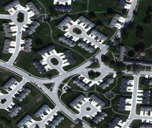
(a) Ortho View

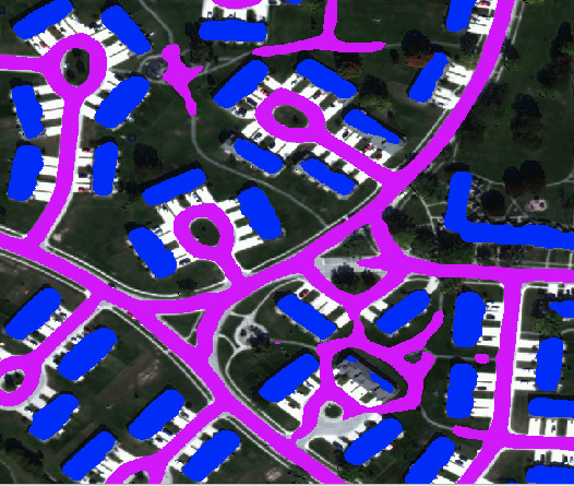
(b) Predicted Labels

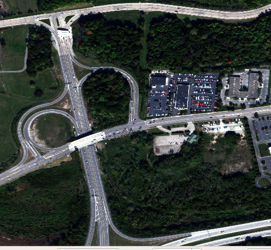
(c) Ortho View

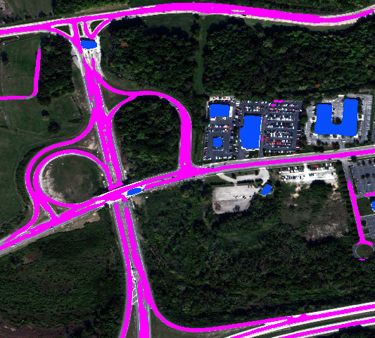
(d) Predicted Labels

Figure 6: Examples of orthorectified images and semantic labels output by our pipeline. Buildings are marked in blue and roads are marked in magenta.

VI-F Qualitative Results

In Figs. 6, 8 and 9, we show some typical examples of semantic labels output by our CNN. In addition, Fig. 1 highlights how multi-view training can help the CNN to segment challenging buildings such as residential buildings which are often occluded by trees, roofs made of highly reflective surfaces, and small buildings. With respect to segmentation of roads, parking lots pose a difficult challenge because their shapes and spectral signatures are very similar to those of true roads. However, multi-view training is able to learn from the differences caused by the absence and presence of vehicles in images captured on different dates, and this is illustrated in Fig. 7.

Single-View Training
Multi-View Training

Figure 7: Examples illustrating how multi-view training helps to distinguish parking lots from true roads. Predicted road labels are marked in magenta

(a) Ortho View

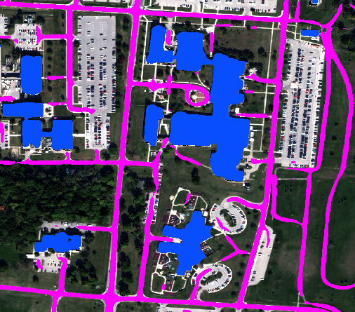
(b) Predicted Labels

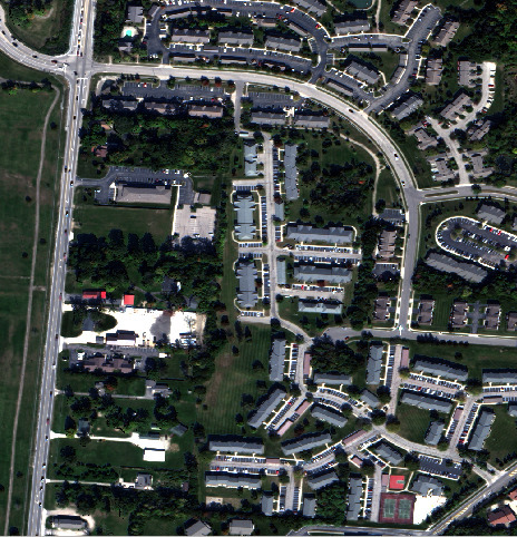
(c) Ortho View

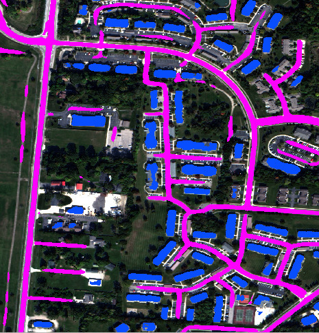
(d) Predicted Labels

Figure 8: Examples of orthorectified images and semantic labels output by our pipeline. Buildings are marked in blue and roads are marked in magenta.

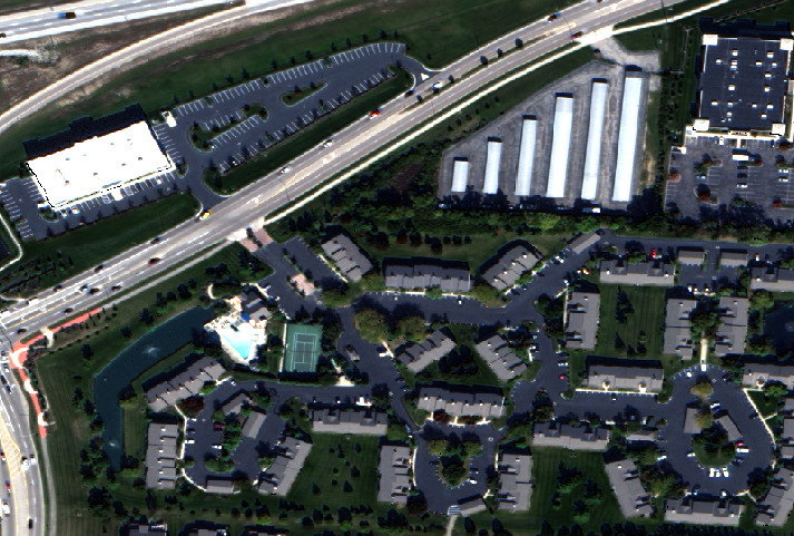
(a) Ortho View

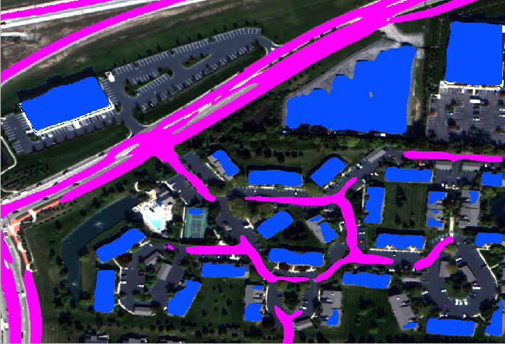
(b) Predicted Labels

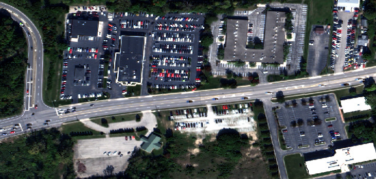
(c) Ortho View

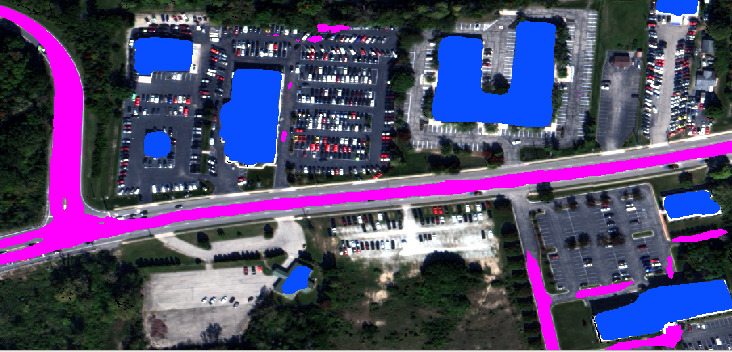
(d) Predicted Labels

Figure 9: Examples of orthorectified images and semantic labels output by our pipeline. Buildings are marked in blue and roads are marked in magenta.

VII Conclusions

We have presented a novel multi-view training paradigm that significantly improves the accuracy of semantic labeling over large geographic areas. The proposed approach intelligently exploits information from multi-view and multi-date images to provide robustness against noise in the training labels. Our approach also speeds up inference, with minimal increase in the GPU memory requirements. Additionally, we have demonstrated that it is possible to use OSM training data to reliably segment large-area geographic regions and off-nadir satellite images without any human supervision. While we have focused on end-to-end automatic labeling of geographic areas, the ideas put forth in this study can be incorporated into other multi-view semantic-segmentation applications. Our research opens up exciting possibilities for multi-view training in related deep-learning tasks such as object detection and panoptic segmentation.

With respect to semantic segmentation, one possible direction of future research is to design an architecture for multi-stage fusion of information from multiple views. More precisely, the features from different views could be combined at multiple layers of a CNN to yield possible improvements in accuracy. On a related note, one could also conduct a study to determine which layers of the SV CNN are influenced by the multi-view loss. Another exciting possibility would be to develop a multi-view framework for off-nadir images. This would require the use of lookup arrays to map between the pixels (in different images) that correspond to the same world point, and to correctly backpropagate gradients. Yet another research direction would be to create normalized DSMs and input them to the multi-view CNN framework. With respect to large-area image alignment and DSM creation, it might be advantageous to investigate the use of a second stage of alignment to resolve the generally small alignment differences between neighboring tiles. In addition, it should be possible to model the errors in the image-alignment and stereo-matching algorithms and subsequently use these models to construct more accurate DSMs. We plan to use our end-to-end automated framework to carry out these studies as part of future research.

Appendix A Alignment of Full-Sized Satellite Images

A-A Tiling

The WorldView-3 images we have used in this study are typically of size $43008\times 38000$ in pixels and cover an area of the ground of size 147 $km^{2}$. In general, images of this size must be broken into image patches, with each image patch covering a tile on the ground. This is made necessary by the following three considerations:

• As we describe in Appendix A-B, the corrections to the camera model calculated for high-precision alignment of the images with one another cannot be assumed to be constant across an entire satellite image.

• The image alignment algorithms usually start with the extraction of tie points from the images. Tie points are the corresponding key points (like those yielded by interest operators like SIFT and SURF) in pairs of images. The computational effort required for extracting the tie points goes up quadratically as the size of the images increases since the key points must be compared across larger images.

• The run-time memory requirements of modern stereo matching algorithms, such as those based on semi-global matching (SGM), can become much too onerous for full sized satellite images.

Based on our experience with WV3 images, we divide the geographic area into overlapping tiles where each tile consists of a central 1 $km^{2}$ main area and a 300 m overlap with each of the four adjoining tiles. This makes for a total area of 2.56 $km^{2}$ for each tile. The image patches that cover tiles of this size are typically of size $5300\times 5300$ in pixels.

Note that the notion of a tile is used only for aligning the images and for constructing a DSM. This DSM is needed to orthorectify the satellite images in order to bring them into correspondence with OSM and with one another. For the CNN-based machine-learning part of the system, we work directly with the whole images and with the OSM for the entire geographic area of interest.

A-B Image-to-Image Alignment

Aligning the satellite images that cover a geographic area means that if we were to project a hypothetical ground point into each of the images, the pixels thus obtained would correspond to their actually recorded positions with sub-pixel precision. If this exercise were to be carried out for WV3 images without first aligning them, the projections in each of the satellite images could be off by as much as 7 pixels from their true locations.

One needs a camera model for the images in order to construct such projections and, for the case of WV3 images, the camera model comes in the form of rational polynomial coefficients (RPCs).

It was shown by Grodecki and Dial [75] that the residual errors in the RPCs, on account of small uncertainties in the measurements related to the position and the attitude of a satellite, can be corrected by adding a constant bias to the projected pixel coordinates of the ground points, provided the area of interest on the ground is not too large. We refer to this as the constant bias assumption for satellite image alignment. We have tested the constant bias assumption mentioned above and verified its validity for image patches of size $5300\times 5300$ (in pixels) for the WV3 images. Fig. 10 presents evidence that the constant bias assumption fails for a full-sized satellite image.

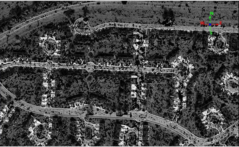
(a)

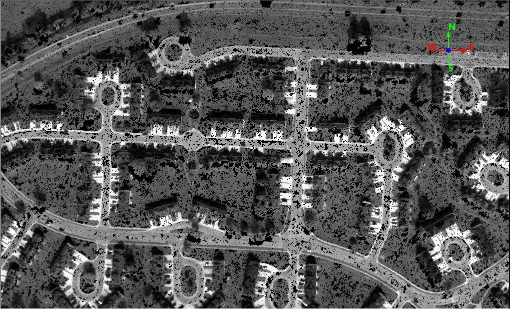
(b)

Figure 10: An example to show why one cannot use a constant bias correction for a full-sized image. At top is the ortho view of a portion of a pairwise point cloud for the constant bias assumption. At bottom is the same for tile-based bias corrections. The points have been colored using the color from the images

A-C Tile-Based Alignment of Large-Area Satellite Images

In order to operate on a large-area basis, we had to extend the standard approach of bundle adjustment that is used to align images. The standard approach consists of: (1) extracting the key points using an operator like SIFT/SURF; (2) establishing correspondences between the key points in pairs of images on the basis of the similarity of their descriptor vectors; (3) using RANSAC to reject the outliers in the set of correspondences (we refer to the surviving correspondences as the pairwise tie points); and (4) estimating the optimum bias corrections for each of the images by the minimization of a reprojection-error based cost function.

We have extended the standard approach by: (1) augmenting the pairwise tie points with multi-image tie points; and (2) adding an $L_{2}$ regularizer to the reprojection-error based cost function. In what follows, we start with the need for multi-image tie points.

Our experience has shown that doing bundle adjustment with the usual pairwise tie points does not yield satisfactory results when the sun angle is just above the horizon or when there is significant snow-cover on the ground. Under these conditions, the decision thresholds one normally uses for extracting the key points from the images often yield an inadequate number of key points. And if one were to lower the decision thresholds, while that does increase the number of key points, it also significantly increases the number of false correspondences between them.

In such images, one gets better results overall by extracting what we refer to as multi-image tie points. The main idea in multi-image tie-point extraction is to construct a graph of the key points detected with lower decision thresholds and subsequently identify the key points that correspond to the same putative world point across multiple images, as opposed to just two images. Unfortunately, multi-image tie points are computationally more expensive than pairwise tie points — roughly three times more expensive. Therefore, they must be used only when needed.

We have developed a “detector” that automatically identifies the tiles that need the extra robustness provided by the multi-image tie points. The detector is based on the rationale that the larger the extent to which each image shares key-point correspondences with all the other images, the more accurate the alignment is likely to be. This rationale is implemented by constructing an attributed graph in which each vertex stands for an image and each edge for the number of key-point correspondences between a pair of images. If we denote the largest connected component in this graph by $C$, the extent to which each node in $C$ is connected with all the other nodes in the same component can then be measured by the following “density”:

$$D(C)=\frac{2|E_{c}|}{|C|(|C|-1)}$$ (7)

where $|E_{c}|$ is the total number of edges and $|C|$ is the total number of vertices in $C$ respectively. The detection for the need for multi-image tie points is carried out by first applying a threshold to $|C|$ and then to $D(C)$. This detection algorithm is described in detail in Fig. 11. The algorithm is motivated by the observation that a dense tie point graph based on pairwise tie points is indicative of good alignment.

After the tie points — pairwise or multi-image — have been identified in all the image patches for a given tile, we apply sparse bundle adjustment (SBA) to them to align the image patches. The implementation of SBA includes an $L_{2}$-regularization term that is added to the reprojection-error based cost function because it significantly increases the overall global accuracy of the alignment. The only remaining issue with regard to the alignment of the images is inter-tile alignment which we discuss in Appendix B-C.

                             An Algorithm to Detect the Need for Multi-Image Tie Points     $S$ – Total number of image patches to be alignedStep 1: Run alignment using pairwise tie points$T_{p}$ – Tie-point graph returned by alignment using pairwise tie points$V$ – Set of all image patches $\{v_{i}\}$. Each image patch is a vertex of $T_{p}$$E$ – Set of all edges $\{e_{ij}\}$. $e_{ij}$ is an edge between the vertices $v_{i}$ and $v_{j}$ with a weight equal to the number of tie points between $v_{i}$ and $v_{j}$$k$, $D_{min}$ – User-specified thresholds$AQ$ – Flag set to True if alignment is of satisfactory quality. Otherwise set to False.Evaluate alignment quality 1. Find the largest connected component $C$ of $T_{p}$. $|C|$ is the number of image patches in $C$. $|E_{c}|$ is the number of edges in $C$. 2. Check how many image patches have been aligned. If $|C|<k\cdot S$, where $0<k<1$, $AQ\leftarrow\textit{False}$. Return AQ 3. Check if $C$ is a tree, i.e., if $|E_{c}|==|C|-1$, $AQ\leftarrow\textit{False}$. Return AQ Explanation – The pushbroom camera model can be closely approximated by an affine camera model, i.e., the camera rays are almost parallel. Therefore, if $C$ is a tree, then for each pair of image patches, the two image patches might be well aligned with each other. However, distinct pairs might not be aligned with one another. 4. Check the sparsity of $C$. $D(C)$ is the density of $C$. $D(C)=\frac{2|E_{c}|}{|C|(|C|-1)}$ If $D(C)<D_{min}$, $AQ\leftarrow\textit{False}$. Return AQ Step 2: If $AQ==\textit{False}$, rerun alignment using multi-image tie points

Figure 11: An algorithm to detect the need for multi-image tie points

Appendix B Creating a Tile-Level DSM

B-A Stereo Matching

As a first step towards constructing a DSM, stereo matching is carried out in a pairwise manner. Similar to the study reported in [64], pairs of images are selected based on heuristics such as the difference in view angles, difference in sun angles, time of acquisition, absolute view angle, etc. In addition, images are selected to cover as wide an azimuth-angle distribution as possible. We err on the side of caution and select a minimum of 40 and a maximum of 80 pairs per tile. For each selected pair, the images are rectified using the approach described by the study in [76].

For stereo matching, we use the hierarchical tSGM algorithm [70] with some enhancements to improve matching accuracy and speed. Specifically, we modify the penalty parameters in the matching cost function as described by the work in [77]. We noticed that this improves accuracy near the edges of elevated structures. The second improvement is to use the SRTM (Shuttle Radar Topography Mission) DEM (Digital Elevation Model) [78] that provides coarse terrain elevation information at a low resolution (30 m). This DEM does not contain the heights of buildings. We use the DEM to better initialize the disparity search range for every point in the disparity volume through a novel procedure that we refer to as “DEM-Sculpting”. Additional details regarding “DEM-Sculpting” can be found in our work described in [65]. This improves accuracy and speeds up stereo matching. Additionally we use a guided bilateral filter for post-processing. With these additions, the matching algorithm is able to handle varying landscapes across a large area.

B-B Pairwise Point-Cloud Creation and Fusion

The disparity maps and corrected RPCs are then used to construct pairwise point clouds. Since the images have already been aligned, the corresponding point clouds are also aligned and can be fused without any further 3D alignment. At each grid point in a tile, the median of the top $Y$ values is retained as the height at that point, where $Y$ is an empirically chosen parameter. Subsequently, median filtering and morphological and boundary based hole-filling techniques are applied.

B-C Merging Tile-Level DSMs

On account of the high absolute alignment precision achieved by using the $L_{2}$ regularization term in the bundle adjustment logic, our experience shows that nothing further needs to be done for merging the tile-level DSMs into a larger DSM. To elaborate, the statistics of the differences in the elevations at the tile boundaries are shown in Table VI in Appendix E-B. We see that the median absolute elevation difference at the tile boundaries is less than 0.5 m – an error that is much too small to introduce noticeable errors in orthorectification. We crop out the center 1 $km^{2}$ region from each DSM tile and place it in the coordinate frame of the larger DSM. This sidesteps the need to resolve any noise-induced variations in the overlapping regions.

Appendix C Generating Training Data using Pansharpened Images and OSM

C-A Pansharpening and Orthorectification

Using the fused DSM as the elevation map, the system is now ready for orthorectifying the satellite images that cover the geographic area. Orthorectification means that you map the pixel values in the images to their corresponding ground-based points in the geographic area of interest. What the system actually orthorectifies are the pansharpened versions of the images — these being the highest resolution panchromatic images (meaning grayscale images) that are assigned multispectral values from the lower resolution multispectral data.

Orthorectification of an off-nadir image can lead to “nodata” regions on the ground if the pixels corresponding to those regions are occluded in the image by tall structures. Our system automatically delineates such regions with a mask that is subsequently used during training of the CNN to prevent gradients at those points from being backpropagated. Each orthorectified image is resampled at a resolution of 0.5 m. More details on orthorectification can be found in Appendix D.

C-B Aligning OSM with Orthorectified Images

This module addresses the noise arising from any misalignments between the OSM and the orthorectified images. Our framework incorporates the following two strategies to align the OSM with the orthorectified images:

1. Using Buildings: First, the system subtracts the DEM from the constructed DSM to extract coarse building footprints. Subsequently, these building footprints are used to align the orthorectified images with the OSM using Normalized Cross Correlation (NCC). This strategy has proved useful in areas with inadequate OSM road labels.

2. Using Roads: First, the system uses the “Red Edge” and “Coastal” bands to calculate the Non-Homogeneous Feature Difference (NHFD) [79], [80] for each point in the orthorectified image and subsequently applies thresholds to the NHFD values to detect coarse road footprints. The NHFD is calculated using the formula:

   $$\text{NHFD}=\frac{(\text{Red Edge - Coastal})}{(\text{Red Edge + Coastal})}$$ (8)

   Subsequently, the roads (noisy obviously) are aligned with the OSM roads using NCC. The system uses this strategy in rural areas that may not contain the buildings needed for the previous approach to work.

After alignment, the OSM vectors are converted to raster format with the same resolution as in the orthorectified images. Thus there is a label for each geographic point in the orthorectified images. The OSM roads are thickened to have a constant width of 8 m.

Fig. 12 shows misaligned and aligned OSM vectors. It should be noted that some residual alignment error does persist. We plan to improve this module by aligning each building/road separately.

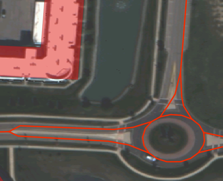
(a)

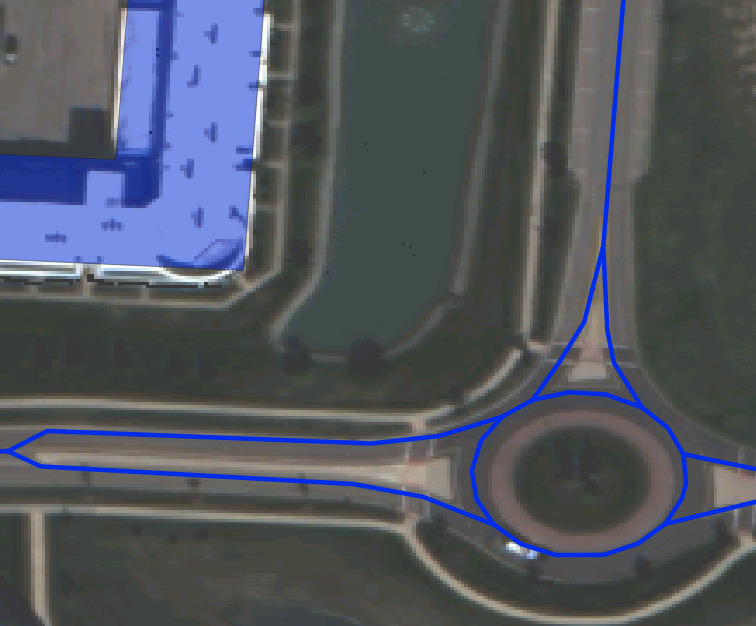
(b)

Figure 12: This figure shows typical results obtained by aligning the orthorectified images with OSM. What is shown in red at left are the unaligned OSM vectors, and what is in blue at right are the aligned versions of the same.

Appendix D True Orthorectification Using gwarp++

We can orthorectify the pansharpened images using the fused DSM as the elevation map. Orthorectification is the process of mapping the pixel values in the images to their corresponding points in the geographic area of interest. There is an important distinction to be made between orthorectification and true orthorectification. If a LiDAR point cloud or DSM is not available, the common practice is to orthorectify images by using a DEM as the source of elevation information. Since a DEM does not contain the heights of elevated structures (buildings, trees, etc.), such an orthorectified view will not represent a true nadir view of the ground. For instance, the vertical walls of buildings will be visible in such a view. To create a true ortho view, we need to take the heights of the elevated structures into account. While doing so, we need to detect those portions of the scene that are occluded by taller structures. Obviously these occluded portions will vary depending upon the satellite view angle.

To the best of our knowledge, there are no open-source utilities to create true ortho images using RPCs and DSMs at this time. Therefore, we have developed a utility, which we have named “gwarp++”, to create full-sized true ortho images quickly and efficiently. Interested researchers can download the “gwarp++” software from the link at [2]. We will now provide a brief overview of “gwarp++”.

                       An Algorithmic Description of “gwarp++” for True Orthorectification     $\phi$ – Latitude, $\lambda$ – Longitude, $h$ – height$\phi_{\text{step}}$ – Latitude step size, $\lambda_{\text{step}}$ – Longitude step size, $h_{\text{step}}$ – Height step sizeImage${}_{\text{Patch}}$ – Off-Nadir image patch$L$ – Length of Image${}_{\text{Patch}}$ in pixels, $W$ – Width of Image${}_{\text{Patch}}$ in pixels$LT\leftarrow Zeros(W,L)$ {// Initialize lookup table to zeros}OutArray – Output array for the orthorectified gridStep 1: Find the extents of the tile spanned by the image patch$(\phi_{\text{min}},\lambda_{\text{max}})$ – Top-left corner of the tile$(\phi_{\text{max}},\lambda_{\text{min}})$ – Bottom-right corner of the tileStep 2: Project points into Image${}_{\text{Patch}}$ and update $LT$   for $\phi=\phi_{\text{min}}\ ;\ \phi\ \leq\phi_{\text{max}}\ ;\ \phi=\phi+\phi_{\text{step}}$ do      for $\lambda=\lambda_{\text{max}}\ ;\ \lambda\ \geq\lambda_{\text{min}}\ ;\ \lambda\ =\lambda-\lambda_{\text{step}}$ do          $h\leftarrow\text{DSM}(\phi,\lambda)$$h_{\text{ground}}\leftarrow\text{DEM}(\phi,\lambda)$         for $h^{\prime}=\ h\ ;\ h^{\prime}\geq h_{\text{ground}}\ ;\ h^{\prime}=h^{\prime}-h_{\text{step}}$ do             $(s,l)\leftarrow$ Proj${}_{\text{RPC}}(\phi,\lambda,h^{\prime})$ {// Proj${}_{\text{RPC}}$ denotes the RPC equations used to project the 3D point into the image}            if $LT(s,l)<h^{\prime}$ then                $LT(s,l)\leftarrow h^{\prime}$            end if         end for      end for   end forStep 3: Create OutArray with a second pass over the grid   for $\phi=\phi_{\text{min}}\ ;\ \phi\ \leq\phi_{\text{max}}\ ;\ \phi=\phi+\phi_{\text{step}}$ do      for $\lambda=\lambda_{\text{max}}\ ;\ \lambda\ \geq\lambda_{\text{min}}\ ;\ \lambda\ =\lambda-\lambda_{\text{step}}$ do          $h\leftarrow\text{DSM}(\phi,\lambda)$$(s,l)\leftarrow$ Proj${}_{\text{RPC}}(\phi,\lambda,h)$         if $LT(s,l)>h+\gamma$ then            OutArray$(\phi,\lambda)\leftarrow$ NODATA         else            OutArray$(\phi,\lambda)\leftarrow$ Image${}_{\text{Patch}}(s,l)$ {// Can also interpolate values}         end if      end for   end for

Figure 13: An algorithmic description of “gwarp++” for true orthorectification

We will first discuss the case of orthorectifying an image patch (that belongs to a single tile) with the help of a DSM. Consider two points W${}_{1}=(\phi_{1},\lambda_{1},h_{1})$ and W${}_{2}=(\phi_{2},\lambda_{2},h_{2})$ that both project to the same pixel coordinates in the image patch. $\phi$, $\lambda$ and $h$ denote the latitude, longitude and height coordinates respectively. If $h_{2}>h_{1}$, it means that W₁ is occluded by W₂. This is the core idea that “gwarp++” uses to detect the occluded “nodata” points.

Now, consider a single world point W $=(\phi,\lambda,h)$, where $h$ is the height value from the DSM. Let $h_{\text{ground}}$ be the corresponding height value in the DEM. The DEM gives us a rough estimate of the height of the ground. It is possible to use more sophisticated techniques, such as the one described by the study in [81], to directly estimate the elevation of the ground from the DSM. The DEM is sufficient for our application. Instead of just projecting W into the image patch, “gwarp++” projects a set of points

$$\hskip 108.405pt\mathcal{W^{\prime}}=\big{\{}(\phi,\lambda,h^{\prime})\big{\}}\$$

$$\forall\ h^{\prime}\ \epsilon\ [\ h,\ h-h_{\text{step}},\ h-2\cdot h_{\text{step}},...,\ h_{\text{ground}}\ ]$$

where $h_{\text{step}}$ is a user-defined step size. $\mathcal{W^{\prime}}$ is therefore a set of points sampled along the vertical line from W to the ground. To understand the motivation for doing this, it might help to consider the case when W is the corner of the roof of a building. In that case, $\mathcal{W^{\prime}}$ is the set of points along the corresponding vertical building edge from W to the ground. If we apply this procedure to all the points on the roof of a building, we will end up projecting the entire building into the image patch.

We now describe the implementation of “gwarp++” below. The algorithm is summarized in Fig. 13.

1. “gwarp++” starts out by dividing the tile into a 2D grid of world points. The grid is 2D in the sense that only the longitude and the latitude coordinates are considered. The extents of this grid can be determined in an iterative fashion by using the RPC equations and the pixel coordinates of the corners of the image patch. The distance between the points of this grid is a user-defined parameter.

2. Using the height values from the DSM, for each point in the grid, “gwarp++” projects a set of points into the image patch as explained above. For each pixel in the image patch, a lookup table “$LT$” stores the maximum height, with the maximum being computed across all the points that project into this pixel. This procedure is repeated for all the points in the 2D grid.

3. At this stage, for each point J in the 2D grid, we know three things:

   • $h_{J}$ – The DSM height value at J

   • $(s,l)$ – The pixel into which J projects after assigning J an elevation value of $h_{J}$

   • $LT(s,l)$ – The maximum height of a world point that projects into $(s,l)$

   If $LT(s,l)\ >h_{J}$, we can conclude that J is occluded by some other world point that has a height value of $LT(s,l)$.

4. Therefore, using a second pass over all the points of the 2D grid, “gwarp++” marks the occluded points with a “NODATA” value. In practice, to account for quantization errors and the noise in the DSM, “gwarp++” checks if $LT(s,l)\ >h_{J}\ +\ \gamma$ where $\gamma$ is chosen appropriately.

To orthorectify the full-sized image, we orthorectify each image patch using its corrected RPCs and the large-area DSM. The orthorectified image patches are then mosaiced into a full-sized orthorectified image during which the overlapping portions between the image patches are discarded.

“gwarp++” is written in C++. It has the nice property of being massively parallel since the projection for each point can be carried out independently and since each tile can be processed independently. This parallelism is exploited at both stages. For each image patch, OpenMP [82] is used to process the points in parallel. And the different image patches are themselves orthorectified in parallel by different virtual machines running on a cloud-based framework.

For our application, each full-sized orthorectified image is resampled at a resolution of 0.5 m. Furthermore, the occluded points are delineated with a mask that is subsequently used during training of the CNN to prevent gradients at those points from being backpropagated.

D-A Accuracy of “gwarp++”

We conclude our discussion on true orthorectification with a few remarks on the accuracy of the orthorectified images produced by “gwarp++”.

3D vs 2.5D: For each point W, “gwarp++” considers points along the vertical line from W to the ground. This is not a good strategy for buildings that possess more exotic shapes such as spherical water towers or buildings with walls that slope inwards. In these cases “gwarp++” can incorrectly mark some points as occluded points. The only way to handle such cases is by using a 3D point cloud instead of a 2.5D DSM, which is beyond the scope of our discussion.

Error Propagation: Errors in the RPCs and errors in the DSM will translate into errors in the orthorectified images. However, in our application, these errors are largely drowned out by the errors in the OSM labels. Nevertheless, it might be useful to study how these errors propagate, which we leave for future work.

Appendix E Quantitative Evaluation of Alignment

E-A Image-to-Image Alignment

We use multiple metrics to evaluate the quality of alignment. Table IV shows the average reprojection error across tiles (and images) for both regions, before and after alignment. Average reprojection error goes down from 5-7 pixels to 0.3 pixels for both regions.

TABLE IV: Average reprojection error in pixels across tiles and images in Ohio and California

Region		Mean	Variance
Ohio	Unaligned	6.70	0.180
	Aligned	0.30	0.003
California	Unaligned	5.71	0.280
	Aligned	0.32	0.001

Since pushbroom sensors can be closely approximated by affine cameras with parallel rays, reprojection error alone does not give the complete picture. For our second metric, we manually annotate tie points in 31 out of 32 images over a 1 km² region in Ohio and in all 32 images over a 2 km² region in California. Within these regions, we measure the pairwise alignment errors for all possible pairs of images and report them in Table V. One can observe that most of the pairs are aligned with subpixel error. This is a much harder metric than the mean reprojection error. It is important to use this metric especially since stereo matching requires subpixel alignment accuracy. The good quality of alignment across the large region is also reflected in the high quality of the DSM and the semantic labeling metrics.

TABLE V: Pairwise alignment error statistics using manually annotated groundtruth for Ohio and California

Region	No. of pairs with error $<1$ pixel	No. of pairs with error $<2$ pixels	Total No. of pairs
Ohio	417	455	465
California	484	496	496

E-B Inter-Tile Alignment

Due to the high absolute alignment precision achieved by using the $L_{2}$ regularization term in the bundle-adjustment logic, it turns out that the tile-level DSMs are well aligned with one another. Table VI shows the statistics of the differences in the elevations at the tile boundaries. It can be seen that the median absolute elevation difference at the tile boundaries is less than 0.5 m – an error that is much too small to introduce noticeable errors in orthorectification.

TABLE VI: Median of the absolute differences in elevation, and median of the rms value of the differences in elevation at the tile boundaries

Region	Median absolute Z diff	Median RMS of Z diff
Ohio	0.42 m	0.72 m
California	0.47 m	0.79 m

Appendix F A Distributed Workflow for Stereo Matching and DSM Creation

Creating DSMs for a 100 km² region is the most computationally-intensive and the slowest module in the framework shown in Fig. 3. It is also the module that is most likely to cause “out-of-memory” errors. Therefore, we need to carefully choose some specific design attributes for this module, which we will highlight in this section.

We can leverage the inherent parallelism in stereo matching and in DSM creation by intelligently distributing the tasks across a cloud computing system. The steps for distributed stereo matching and DSM creation are enumerated below and shown in Fig. 14.

1. A captain virtual machine (VM) prepares a list of the selected stereo pairs of image patches for each tile. This is done for all the tiles at the beginning. All the tiles are added to a queue. All the lists are stored on a shared Network Attached Storage (NAS).

2. The captain sends a message to all the worker VMs to start. The captain also assumes the role of a worker at this step.

3. For the first tile in the queue, the workers pull/request a pair of image patches to process. Safeguards are imposed to ensure that each worker gets a unique pair.

4. Each worker attempts to create a pairwise point cloud and subsequently reports the status of its task. Each worker then pull/requests the next unprocessed stereo pair for the current tile. Successfully processed stereo pairs are marked as done.

5. If there are no more unprocessed stereo pairs for this tile then:

   1. The current tile is removed from the queue. All the idle workers except for the captain and the large VMs move on to the next tile in the queue, i.e., to step 3. By a large VM, we mean a VM with more memory and a larger number of CPUs.

   2. All the stereo pairs for which point-cloud creation failed are processed for a second time by the remaining workers. Even if processing fails again, these stereo pairs are marked as done.

6. At this stage, all the selected stereo pairs for the current tile are marked as done. The large VMs join their smaller counterparts on the next tile, i.e., at step 3. The captain alone starts the process of fusing the multiple pairwise point clouds into a single fused DSM for the current tile. After this, the captain also proceeds to join the other VMs in step 3.

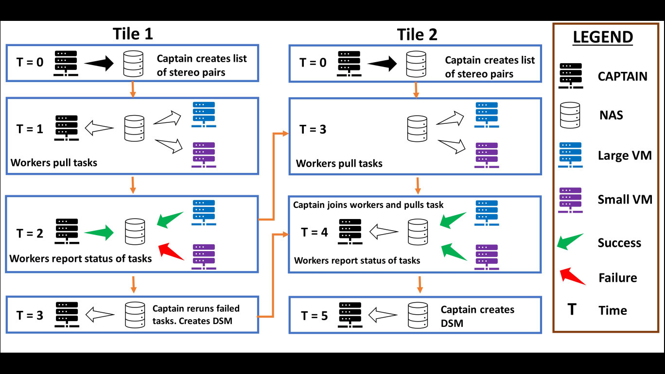
Figure 14: An example to illustrate our distributed stereo-matching and DSM-creation workflow. In this example, there are only 2 tiles and 3 selected stereo pairs for each tile. There are only 3 VMs, a captain, a small VM and a large VM. T indicates the time stamp. Notice how at T = 3, two of the VMs have moved onto Tile 2 whereas the captain stays back to finish processing Tile 1.

A graphic illustration of the above workflow is shown in Fig. 14. For the sake of clarity, in this illustration, we assume that there are only 2 tiles and that there are only 3 selected stereo pairs for each tile. We also assume that there are only 3 VMs, a captain, a small VM and a large VM.

F-A Advantages of this Distributed Workflow

• No VM remains idle except during the last processing stage of the very last tile.

• Failed pairs are processed twice to handle “out-of-memory” errors.

• The intensive process of creating a fused DSM is carried out on the most powerful captain VM.

• Note that we could have opted to use a simpler workflow where all the VMs wait for a fused DSM to be created before proceeding to the next tile. However, our workflow reduces the processing time by a number of days.

  For an example, assume that there are 10 VMs and 100 tiles. Also assume that each stereo pair takes 20 minutes to process, that we process 80 pairs per tile and that the point-cloud fusion takes 60 minutes. If all the workers waited for a tile-level DSM to be created before moving on to the next tile, then it would take $\frac{(\frac{80\times 20}{10}+60)}{60}\approx$ 3 hours and 40 minutes to finish processing a single tile. For 100 tiles it would take $\approx$ 15 days and 6 hours.

  Our workflow takes $\frac{(\frac{80\times 20}{10})}{60}\approx$ 2 hours and 40 minutes for a single tile. This is because while the captain is fusing the point clouds for a tile, the other VMs will be processing the next tile. For 100 tiles it would take $\approx$ 11 days and 2 hours, roughly saving us 4 days of processing time.

Bharath Comandur received the Bachelor of Technology degree in Electrical Engineering from the Indian Institute of Technology, Madras in 2012 and obtained his Ph.D. in Computer Engineering from the school of Electrical and Computer Engineering, Purdue University where he was affiliated with the Robot Vision Laboratory. His research interests include computer vision, machine learning, remote sensing and cloud computing.

Avinash C. Kak is a professor of electrical and computer engineering at Purdue University. His research focuses on algorithms, languages, and systems related to wired and wireless camera networks, robotics, computer vision, etc. His coauthored book Principles of Computerized Tomographic Imaging was republished as a classic in applied mathematics by the Society of Industrial and Applied Mathematics. His other coauthored book, Digital Picture Processing, also considered by many to be a classic in computer vision and image processing, was published by Academic Press in 1982. His more recent books were written for his “Objects Trilogy” project. All three books of the Trilogy have been published by John Wiley & Sons. the first, Programming with Objects, came out in 2003, the second, Scripting with Objects, in 2008, and the last, Designing with Objects, in 2015.

References

- [1] OpenStreetMap contributors, “Planet dump retrieved from https://planet.osm.org ,” https://www.openstreetmap.org, 2017.
- [2] “gwarp++,” https://github.com/shallowlearn/gwarp, accessed: 2020-11-25.
- [3] “Flyby Videos of Large-Area DSMs,” https://engineering.purdue.edu/RVL/CORE3D/DSM/, accessed: 2020-11-25.
- [4] “WorldView-3,” https://www.satimagingcorp.com/satellite-sensors/worldview-3/, accessed: 2018-08-06.
- [5] Z. Li, J. D. Wegner, and A. Lucchi, “Topological map extraction from overhead images,” in Proceedings of the IEEE International Conference on Computer Vision, 2019, pp. 1715–1724.
- [6] F. Bastani, S. He, S. Abbar, M. Alizadeh, H. Balakrishnan, S. Chawla, S. Madden, and D. DeWitt, “Roadtracer: Automatic extraction of road networks from aerial images,” in Proceedings of the IEEE Conference on Computer Vision and Pattern Recognition, 2018, pp. 4720–4728.
- [7] F. Bastani, S. He, S. Abbar, M. Alizadeh, H. Balakrishnan, S. Chawla, and S. Madden, “Machine-assisted map editing,” in Proceedings of the 26th ACM SIGSPATIAL International Conference on Advances in Geographic Information Systems, 2018, pp. 23–32.
- [8] H. Chu, D. Li, D. Acuna, A. Kar, M. Shugrina, X. Wei, M.-Y. Liu, A. Torralba, and S. Fidler, “Neural Turtle Graphics for Modeling City Road Layouts,” in The IEEE International Conference on Computer Vision (ICCV), October 2019.
- [9] X. Yang, X. Li, Y. Ye, R. Y. Lau, X. Zhang, and X. Huang, “Road Detection and Centerline Extraction Via Deep Recurrent Convolutional Neural Network U-Net,” IEEE Transactions on Geoscience and Remote Sensing, vol. 57, no. 9, pp. 7209–7220, 2019.
- [10] E. Park et al., “Refining inferred road maps using GANs,” Ph.D. dissertation, Massachusetts Institute of Technology, 2019.
- [11] A. V. Etten, “City-Scale Road Extraction from Satellite Imagery v2: Road Speeds and Travel Times,” in The IEEE Winter Conference on Applications of Computer Vision (WACV), March 2020.
- [12] A. Mosinska, M. Kozinski, and P. Fua, “Joint Segmentation and Path Classification of Curvilinear Structures,” IEEE transactions on pattern analysis and machine intelligence, 2019.
- [13] X. Yang, X. Li, Y. Ye, X. Zhang, H. Zhang, X. Huang, and B. Zhang, “Road Detection via Deep Residual Dense U-Net,” in 2019 International Joint Conference on Neural Networks (IJCNN). IEEE, 2019, pp. 1–7.
- [14] P. Kaiser, J. D. Wegner, A. Lucchi, M. Jaggi, T. Hofmann, and K. Schindler, “Learning Aerial Image Segmentation From Online Maps,” IEEE Transactions on Geoscience and Remote Sensing, vol. 55, no. 11, pp. 6054–6068, Nov 2017.
- [15] Z. Zhang, Q. Liu, and Y. Wang, “Road Extraction by Deep Residual U-Net,” IEEE Geoscience and Remote Sensing Letters, vol. 15, no. 5, pp. 749–753, May 2018.
- [16] S. Saito, Y. Yamashita, and Y. Aoki, “Multiple Object Extraction from Aerial Imagery with Convolutional Neural Networks,” vol. 60, pp. 10 402–1/10 402, 01 2016.
- [17] E. Maggiori, Y. Tarabalka, G. Charpiat, and P. Alliez, “Convolutional Neural Networks for Large-Scale Remote-Sensing Image Classification,” IEEE Transactions on Geoscience and Remote Sensing, vol. 55, no. 2, pp. 645–657, Feb 2017.
- [18] Y. Li, L. Guo, J. Rao, L. Xu, and S. Jin, “Road Segmentation Based on Hybrid Convolutional Network for High-Resolution Visible Remote Sensing Image,” IEEE Geoscience and Remote Sensing Letters, vol. 16, no. 4, pp. 613–617, April 2019.
- [19] J. Chen and A. Zipf, “DeepVGI: Deep Learning with Volunteered Geographic Information,” in WWW, 2017.
- [20] S. Kurath, “OSMDeepOD -Object Detection on Orthophotos with and for VGI,” vol. Volume 2, pp. 173–188, online available: http://www.austriaca.at/?arp=0x00373589 - Last access:12.8.2018. [Online]. Available: http://www.austriaca.at/?arp=0x00373589
- [21] “DeepOSM,” https://github.com/trailbehind/DeepOSM, accessed: 2018-08-06.
- [22] I. Goodfellow, J. Pouget-Abadie, M. Mirza, B. Xu, D. Warde-Farley, S. Ozair, A. Courville, and Y. Bengio, “Generative Adversarial Nets,” in Advances in Neural Information Processing Systems, Z. Ghahramani, M. Welling, C. Cortes, N. Lawrence, and K. Q. Weinberger, Eds., vol. 27. Curran Associates, Inc., 2014, pp. 2672–2680. [Online]. Available: https://proceedings.neurips.cc/paper/2014/file/5ca3e9b122f61f8f06494c97b1afccf3-Paper.pdf
- [23] G. Máttyus, W. Luo, and R. Urtasun, “DeepRoadMapper: Extracting Road Topology from Aerial Images,” in 2017 IEEE International Conference on Computer Vision (ICCV), Oct 2017, pp. 3458–3466.
- [24] L. Zhou, C. Zhang, and M. Wu, “D-LinkNet: LinkNet With Pretrained Encoder and Dilated Convolution for High Resolution Satellite Imagery Road Extraction,” in CVPR Workshops, 2018, pp. 182–186.
- [25] A. Batra, S. Singh, G. Pang, S. Basu, C. Jawahar, and M. Paluri, “Improved road connectivity by joint learning of orientation and segmentation,” in Proceedings of the IEEE Conference on Computer Vision and Pattern Recognition, 2019, pp. 10 385–10 393.
- [26] S. Singh, A. Batra, G. Pang, L. Torresani, S. Basu, M. Paluri, and C. Jawahar, “Self-Supervised Feature Learning for Semantic Segmentation of Overhead Imagery,” in BMVC, vol. 1, no. 2, 2018, p. 4.
- [27] G. Rotich, S. Aakur, R. Minetto, M. P. Segundo, and S. Sarkar, “Using Semantic Relationships among Objects for Geospatial Land Use Classification,” in 2018 IEEE Applied Imagery Pattern Recognition Workshop (AIPR). IEEE, 2018, pp. 1–7.
- [28] G. Rotich, R. Minetto, and S. Sarkar, “Resource-constrained simultaneous detection and labeling of objects in high-resolution satellite images,” arXiv preprint arXiv:1810.10110, 2018.
- [29] D. Costea, A. Marcu, E. Slusanschi, and M. Leordeanu, “Roadmap Generation Using a Multi-Stage Ensemble of Deep Neural Networks With Smoothing-Based Optimization.” in CVPR Workshops, 2018, pp. 220–224.
- [30] I. Demir, K. Koperski, D. Lindenbaum, G. Pang, J. Huang, S. Basu, F. Hughes, D. Tuia, and R. Raskar, “DeepGlobe 2018: A Challenge to Parse the Earth through Satellite Images,” CoRR, vol. abs/1805.06561, 2018. [Online]. Available: http://arxiv.org/abs/1805.06561
- [31] “SpaceNet on Amazon Web Services (AWS). ”Datasets.” The SpaceNet Catalog. Last modified April 30, 2018.” https://spacenetchallenge.github.io/datasets/datasetHomePage.html, accessed: 2018-08-06.
- [32] M. Bosch, K. Foster, G. Christie, S. Wang, G. D. Hager, and M. Brown, “Semantic stereo for incidental satellite images,” in 2019 IEEE Winter Conference on Applications of Computer Vision (WACV). IEEE, 2019, pp. 1524–1532.
- [33] H. R. Goldberg, S. Wang, G. A. Christie, and M. Z. Brown, “Urban 3D challenge: building footprint detection using orthorectified imagery and digital surface models from commercial satellites,” in Geospatial Informatics, Motion Imagery, and Network Analytics VIII, K. Palaniappan, P. J. Doucette, and G. Seetharaman, Eds., vol. 10645, International Society for Optics and Photonics. SPIE, 2018, pp. 12 – 31. [Online]. Available: https://doi.org/10.1117/12.2304682
- [34] M. Brown, H. Goldberg, K. Foster, A. Leichtman, S. Wang, S. Hagstrom, M. Bosch, and S. Almes, “Large-scale public lidar and satellite image data set for urban semantic labeling,” in Laser Radar Technology and Applications XXIII, M. D. Turner and G. W. Kamerman, Eds., vol. 10636, International Society for Optics and Photonics. SPIE, 2018, pp. 154 – 167. [Online]. Available: https://doi.org/10.1117/12.2304403
- [35] “IEEE Data Fusion Contest,” http://www.grss-ieee.org/community/technical-committees/data-fusion/data-fusion-contest/, accessed: 2018-08-06.
- [36] A. Lagrange, B. L. Saux, A. Beaupère, A. Boulch, A. Chan-Hon-Tong, S. Herbin, H. Randrianarivo, and M. Ferecatu, “Benchmarking classification of earth-observation data: From learning explicit features to convolutional networks,” in 2015 IEEE International Geoscience and Remote Sensing Symposium (IGARSS), July 2015, pp. 4173–4176.
- [37] “ISPRS-2D Dataset,” http://www2.isprs.org/commissions/comm3/wg4/semantic-labeling.html, accessed: 2018-08-06.
- [38] S. Wang, M. Bai, G. Máttyus, H. Chu, W. Luo, B. Yang, J. Liang, J. Cheverie, S. Fidler, and R. Urtasun, “TorontoCity: Seeing the World with a Million Eyes,” CoRR, vol. abs/1612.00423, 2016. [Online]. Available: http://arxiv.org/abs/1612.00423
- [39] G. Xia, X. Bai, J. Ding, Z. Zhu, S. J. Belongie, J. Luo, M. Datcu, M. Pelillo, and L. Zhang, “DOTA: A Large-scale Dataset for Object Detection in Aerial Images,” CoRR, vol. abs/1711.10398, 2017. [Online]. Available: http://arxiv.org/abs/1711.10398
- [40] “Geospatial Repository and Data Management System,” https://griduc.rsgis.erdc.dren.mil/griduc, accessed: 2018-08-06.
- [41] N. Yokoya, P. Ghamisi, J. Xia, S. Sukhanov, R. Heremans, I. Tankoyeu, B. Bechtel, B. Le Saux, G. Moser, and D. Tuia, “Open Data for Global Multimodal Land Use Classification: Outcome of the 2017 IEEE GRSS Data Fusion Contest,” IEEE Journal of Selected Topics in Applied Earth Observations and Remote Sensing, vol. 11, no. 5, pp. 1363–1377, May 2018.
- [42] L. Ma, J. Stückler, C. Kerl, and D. Cremers, “Multi-view deep learning for consistent semantic mapping with RGB-D cameras,” in 2017 IEEE/RSJ International Conference on Intelligent Robots and Systems (IROS), Sep. 2017, pp. 598–605.
- [43] J. Xiao and L. Quan, “Multiple view semantic segmentation for street view images,” in 2009 IEEE 12th International Conference on Computer Vision, Sep. 2009, pp. 686–693.
- [44] L. Ge, H. Liang, J. Yuan, and D. Thalmann, “Robust 3D Hand Pose Estimation in Single Depth Images: From Single-View CNN to Multi-View CNNs,” in The IEEE Conference on Computer Vision and Pattern Recognition (CVPR), June 2016.
- [45] H. Su, S. Maji, E. Kalogerakis, and E. Learned-Miller, “Multi-View Convolutional Neural Networks for 3D Shape Recognition,” in The IEEE International Conference on Computer Vision (ICCV), December 2015.
- [46] C. R. Qi, H. Su, M. Niessner, A. Dai, M. Yan, and L. J. Guibas, “Volumetric and Multi-View CNNs for Object Classification on 3D Data,” in The IEEE Conference on Computer Vision and Pattern Recognition (CVPR), June 2016.
- [47] A. Mortazi, R. Karim, K. Rhode, J. Burt, and U. Bagci, “CardiacNET: Segmentation of Left Atrium and Proximal Pulmonary Veins from MRI Using Multi-view CNN,” in Medical Image Computing and Computer-Assisted Intervention, MICCAI 2017, M. Descoteaux, L. Maier-Hein, A. Franz, P. Jannin, D. L. Collins, and S. Duchesne, Eds. Cham: Springer International Publishing, 2017, pp. 377–385.
- [48] G. Carneiro, J. Nascimento, and A. P. Bradley, “Unregistered Multiview Mammogram Analysis with Pre-trained Deep Learning Models,” in Medical Image Computing and Computer-Assisted Intervention – MICCAI 2015, N. Navab, J. Hornegger, W. M. Wells, and A. F. Frangi, Eds. Cham: Springer International Publishing, 2015, pp. 652–660.
- [49] J. Han, H. Chen, N. Liu, C. Yan, and X. Li, “CNNs-based RGB-D saliency detection via cross-view transfer and multiview fusion,” IEEE transactions on cybernetics, vol. 48, no. 11, pp. 3171–3183, 2017.
- [50] G. Kang, K. Liu, B. Hou, and N. Zhang, “3D multi-view convolutional neural networks for lung nodule classificationq,” PLOS ONE, vol. 12, no. 11, pp. 1–21, 11 2017. [Online]. Available: https://doi.org/10.1371/journal.pone.0188290
- [51] M. Elhoseiny, T. El-Gaaly, A. Bakry, and A. M. Elgammal, “A Comparative Analysis and Study of Multiview CNN Models for Joint Object Categorization and Pose Estimation,” in ICML, 2016.
- [52] F. P. S. Luus, B. P. Salmon, F. van den Bergh, and B. T. J. Maharaj, “Multiview Deep Learning for Land-Use Classification,” IEEE Geoscience and Remote Sensing Letters, vol. 12, no. 12, pp. 2448–2452, Dec 2015.
- [53] A. Dai and M. Niessner, “3DMV: Joint 3D-Multi-View Prediction for 3D Semantic Scene Segmentation,” in The European Conference on Computer Vision (ECCV), September 2018.
- [54] E. Kalogerakis, M. Averkiou, S. Maji, and S. Chaudhuri, “3D shape segmentation with projective convolutional networks,” in Proceedings of the IEEE Conference on Computer Vision and Pattern Recognition, 2017, pp. 3779–3788.
- [55] S. Saha, F. Bovolo, and L. Bruzzone, “Unsupervised Multiple-Change Detection in VHR Multisensor Images Via Deep-Learning Based Adaptation,” in IGARSS 2019 - 2019 IEEE International Geoscience and Remote Sensing Symposium, 2019, pp. 5033–5036.
- [56] Zhu, Jun-Yan and Park, Taesung and Isola, Phillip and Efros, Alexei A, “Unpaired Image-to-Image Translation using Cycle-Consistent Adversarial Networks,” in Computer Vision (ICCV), 2017 IEEE International Conference on, 2017.
- [57] P. d’Angelo, D. Cerra, S. M. Azimi, N. Merkle, J. Tian, S. Auer, M. Pato, R. de los Reyes, X. Zhuo, K. Bittner, T. Krauss, and P. Reinartz, “3D Semantic Segmentation from Multi-View Optical Satellite Images,” in IGARSS 2019 - 2019 IEEE International Geoscience and Remote Sensing Symposium, July 2019, pp. 5053–5056.
- [58] B. Le Saux, N. Yokoya, R. Hansch, M. Brown, and G. Hager, “2019 data fusion contest [technical committees],” IEEE Geoscience and Remote Sensing Magazine, vol. 7, no. 1, pp. 103–105, 2019.
- [59] M. J. Leotta, C. Long, B. Jacquet, M. Zins, D. Lipsa, J. Shan, B. Xu, Z. Li, X. Zhang, S.-F. Chang, M. Purri, J. Xue, and K. Dana, “Urban Semantic 3D Reconstruction From Multiview Satellite Imagery,” in The IEEE Conference on Computer Vision and Pattern Recognition (CVPR) Workshops, June 2019.
- [60] R. Qin, “Automated 3D recovery from very high resolution multi-view satellite images,” CoRR, vol. abs/1905.07475, 2019. [Online]. Available: http://arxiv.org/abs/1905.07475
- [61] G. Kuschk, “LARGE SCALE URBAN RECONSTRUCTION FROM REMOTE SENSING IMAGERY,” ISPRS - International Archives of the Photogrammetry, Remote Sensing and Spatial Information Sciences, vol. XL-5/W1, pp. 139–146, 2013. [Online]. Available: https://www.int-arch-photogramm-remote-sens-spatial-inf-sci.net/XL-5-W1/139/2013/
- [62] D. Shean, O. Alexandrov, Z. Moratto, B. Smith, I. Joughin, C. Porter, and P. Morin, “An automated, open-source pipeline for mass production of digital elevation models (DEMs) from very-high-resolution commercial stereo satellite imagery,” ISPRS Journal of Photogrammetry and Remote Sensing, vol. 116, pp. 101–117, 6 2016.
- [63] O. C. Ozcanli, Y. Dong, J. L. Mundy, H. Webb, R. Hammoud, and V. Tom, “A comparison of stereo and multiview 3-D reconstruction using cross-sensor satellite imagery,” in 2015 IEEE Conference on Computer Vision and Pattern Recognition Workshops (CVPRW), June 2015, pp. 17–25.
- [64] G. Facciolo, C. D. Franchis, and E. Meinhardt-Llopis, “Automatic 3D Reconstruction from Multi-date Satellite Images,” in 2017 IEEE Conference on Computer Vision and Pattern Recognition Workshops (CVPRW), July 2017, pp. 1542–1551.
- [65] S. Patil, T. Prakash, B. Comandur, and A. C. Kak, “A Comparative Evaluation of SGM Variants (including a New Variant, tMGM) for Dense Stereo Matching,” CoRR, vol. abs/1911.09800, 2019. [Online]. Available: http://arxiv.org/abs/1911.09800
- [66] K. Gong and D. Fritsch, “POINT CLOUD AND DIGITAL SURFACE MODEL GENERATION FROM HIGH RESOLUTION MULTIPLE VIEW STEREO SATELLITE IMAGERY,” ISPRS - International Archives of the Photogrammetry, Remote Sensing and Spatial Information Sciences, vol. XLII-2, pp. 363–370, 2018. [Online]. Available: https://www.int-arch-photogramm-remote-sens-spatial-inf-sci.net/XLII-2/363/2018/
- [67] R. Perko, H. Raggam, and P. M. Roth, “Mapping with Pléiades–End-to-End Workflow,” Remote Sensing, vol. 11, no. 17, 2019. [Online]. Available: https://www.mdpi.com/2072-4292/11/17/2052
- [68] S. Patil, B. Comandur, T. Prakash, and A. C. Kak, “A New Stereo Benchmarking Dataset for Satellite Images,” CoRR, vol. abs/1907.04404, 2019. [Online]. Available: http://arxiv.org/abs/1907.04404
- [69] R. S. Gargees and G. J. Scott, “Deep Feature Clustering for Remote Sensing Imagery Land Cover Analysis,” IEEE Geoscience and Remote Sensing Letters, vol. 17, no. 8, pp. 1386–1390, 2020.
- [70] M. Rothermel, “Development of a SGM-based multi-view reconstruction framework for aerial imagery,” Dissertation, University of Stuttgart, 2016.
- [71] O. Ronneberger, P.Fischer, and T. Brox, “U-Net: Convolutional Networks for Biomedical Image Segmentation,” in Medical Image Computing and Computer-Assisted Intervention (MICCAI), ser. LNCS, vol. 9351. Springer, 2015, pp. 234–241, (available on arXiv:1505.04597 [cs.CV]). [Online]. Available: http://lmb.informatik.uni-freiburg.de/Publications/2015/RFB15a
- [72] S. Ioffe and C. Szegedy, “Batch Normalization: Accelerating Deep Network Training by Reducing Internal Covariate Shift,” CoRR, vol. abs/1502.03167, 2015. [Online]. Available: http://arxiv.org/abs/1502.03167
- [73] Y. Zhu, K. Sapra, F. A. Reda, K. J. Shih, S. Newsam, A. Tao, and B. Catanzaro, “Improving Semantic Segmentation via Video Propagation and Label Relaxation,” in Proceedings of the IEEE Conference on Computer Vision and Pattern Recognition, 2019, pp. 8856–8865.
- [74] M. Cordts, M. Omran, S. Ramos, T. Rehfeld, M. Enzweiler, R. Benenson, U. Franke, S. Roth, and B. Schiele, “The Cityscapes Dataset for Semantic Urban Scene Understanding,” in Proc. of the IEEE Conference on Computer Vision and Pattern Recognition (CVPR), 2016.
- [75] J. Grodecki and G. Dial, “Block Adjustment of High-Resolution Satellite Images Described by Rational Polynomials,” Photogrammetric Engineering & Remote Sensing, vol. 69, no. 1, pp. 59–68, 2003. [Online]. Available: https://www.ingentaconnect.com/content/asprs/pers/2003/00000069/00000001/art00004
- [76] J. Oh, W. H. Lee, C. K. Toth, D. A. Grejner-Brzezinska, and C. Lee, “A piecewise approach to epipolar resampling of pushbroom satellite images based on RPC,” Photogrammetric Engineering & Remote Sensing, vol. 76, no. 12, pp. 1353–1363, 2010.
- [77] J. Zbontar and Y. LeCun, “Stereo matching by training a convolutional neural network to compare image patches,” Journal of Machine Learning Research, vol. 17, pp. 1–32, 2016.
- [78] “SRTM DEM,” https://www2.jpl.nasa.gov/srtm/, accessed: 2018-08-06.
- [79] A. F. Wolf, “Using WorldView-2 Vis-NIR multispectral imagery to support land mapping and feature extraction using normalized difference index ratios,” in Algorithms and Technologies for Multispectral, Hyperspectral, and Ultraspectral Imagery XVIII, S. S. Shen and P. E. Lewis, Eds., vol. 8390, International Society for Optics and Photonics. SPIE, 2012, pp. 188 – 195. [Online]. Available: https://doi.org/10.1117/12.917717
- [80] T. Prakash and A. C. Kak, “Active learning for designing detectors for infrequently occurring objects in wide-area satellite imagery,” Computer Vision and Image Understanding, vol. 170, pp. 92 – 108, 2018. [Online]. Available: http://www.sciencedirect.com/science/article/pii/S1077314218300390
- [81] W. Zhang, J. Qi, P. Wan, H. Wang, D. Xie, X. Wang, and G. Yan, “An Easy-to-Use Airborne LiDAR Data Filtering Method Based on Cloth Simulation,” Remote Sensing, vol. 8, no. 6, p. 501, Jun 2016. [Online]. Available: http://dx.doi.org/10.3390/rs8060501
- [82] “OpenMP,” https://www.openmp.org/, accessed: 2020-05-20.