Renyi entropy as a measure of cosmic homogeneity

Abstract

We propose a method for testing homogeneity in three dimensional spatial distributions using Renyi entropy. We apply the proposed method to data from cosmological N-body simulations and Monte Carlo simulations of homogeneous Poisson point process. We show that the method can effectively characterize the inhomogeneities and identify any transition scale to homogeneity, if present in such distributions. The proposed method can be used to study the cosmic homogeneity in present and future generation galaxy redshift surveys.

1 Introduction

The assumption of statistical homogeneity and isotropy of the Universe on sufficiently large scales, known as the Cosmological principle, is fundamental to modern cosmology. The principle can not be proved in a strictly mathematical sense and was introduced in cosmology largely due to its great aesthetic appeal and simplicity. It allows us to mathematically describe the global structure of the Universe using FRW space-time geometry. We rely on the FRW geometry while analyzing and interpreting data from various cosmological observations. So the assumption is of paramount importance for our current understanding of the Universe and the validity of this assumption must be tested with different observations. Besides, inhomogeneities may also play an important role in explaining the observed cosmic acceleration through the backreaction mechanism [1, 2, 3, 4, 5].

The isotropy of the Universe is supported by a multitude of observations such as CMBR [6, 7, 8], radio sources [9, 10], X-ray background [11, 12, 13], Gamma ray bursts [14, 15], supernovae [16, 17] and galaxies [18, 19, 20]. However these observations alone can not assert the large-scale statistical homogeneity of the Universe. Such a validation is only possible if we believe that our location in the Universe is not a special one.

The observed galaxy distribution is known to exhibit scale invariant features on small scales [21, 22, 23] which resembles fractals. A number of studies [21, 22, 24, 25, 26, 27, 28] claim that such scale-invariant behaviour continues on larger length scales extending out to the scale of the surveys, which indicates that there are no transition scale to homogeneity. Many other studies reaffirm the scale invariant nature of galaxy distribution on small scales but most of them [29, 30, 31, 32, 33, 34, 35, 36, 37, 38, 39, 40, 41] reported a transition to homogeneity on scales $70-150{\,h^{-1}\,{\rm Mpc}}$.

Various observations point out to the existence of structures in the Universe, which extend up to several hundreds of Mpc. The Sloan Great Wall (SGW) in the SDSS galaxy distribution is known to extend over length scales of $\sim 400$ Mpc [42]. The large quasar groups (LQG) in the quasar distribution at $z\sim 1.3$ is known to have a characteristic size of $\sim 500{\,h^{-1}\,{\rm Mpc}}$ [43]. The Eridanus supervoid is believed to stretch across a region, which extends up to $\sim 300$ Mpc [44]. The existence of such large-scale structures may challenge the validity of the cosmological principle and the standard cosmological model. Using Horizon Run 2 simulation, Park et al. [45] show that existence of high density and low density regions of such extent in observations are consistent with $\Lambda$CDM paradigm. It is also important to address the statistical significance of any such structures identified in observations. For instance, Nadathur [39] pointed out that the algorithm used for identification of LQGs yield even larger structures in simulations of a homogeneous Poisson point process.

Most of the traditional methods for testing homogeneity are based on the number counts in spheres centered around galaxies. Multi-fractal analysis [46, 22, 30, 33, 35] of galaxies is one of the most widely used method for testing cosmic homogeneity. It characterizes The scale of homogeneity by studying the scaling of different moments of number counts. In a multi-fractal, different moments of the distribution scale with different scaling exponent. The multi-fractals can be defined based on the Renyi dimension or generalized dimension [47, 48]. However $r\to 0$ limit in these definitions are not meaningful for observed galaxy distributions and it is difficult to measure them accurately [49]. Pandey [50] defined a statistical measure for homogeneity based on the Shannon entropy [51] and used it to measure the scale of homogeneity in the Main Galaxy sample [40], LRG sample [41] and BOSS sample [52] from the SDSS [53]. In information theory, Renyi entropy [54] is one of the families of functionals which quantify the uncertainty or randomness of a system. The Shannon entropy is the limiting case of the Renyi entropy. The Renyi entropies of higher order are more sensitive to the presence of inhomogeneities in a distribution. In the present work, we propose a more general statistical measure of homogeneity based on the Renyi entropy. We apply the proposed method to data from simulations of homogeneous Poisson point process and distributions of particles from N-body simulations. We explore the scope and limitations of the proposed method in studying cosmic homogeneity using the present generation and forthcoming galaxy surveys.

The outline of the paper is as follows: We explain the method of analysis in Section 2 and describe the data in Section 3. We discuss the results and present our conclusions in Section 4.

2 Method of Analysis

Information theory is an interdisciplinary branch of science which owes its origin to a seminal paper [51] by Claude Shannon.

Shannon entropy measures the average information content of a random variable. The Shannon entropy of a discrete random variable $X$ is defined as,

$$H(X) = -\sum^{n}_{i=1}\,p(x_{i})\,\log\,p(x_{i})$$ (2.1)

,where $p(x_{i})$ is the probability of $i^{th}$ event out of a total $n$ outcomes $\{x_{i}:i=1,....n\}$.

The Renyi entropy [54] generalizes Shannon entropy, which was originally proposed by Alfred Renyi in 1961. The Renyi entropy of order $q$ for a random variable $X$ is defined as,

$$S_{q}(X) = \frac{1}{1-q}\,\log\sum^{n}_{i=1}\,p^{q}(x_{i})$$ (2.2)

,where $q\in[0,\infty]$. For $q=0$, we get the maximum entropy which is the logarithm of the size of the support of $p$. The expression given in equation 2.2 is potentially undefined for $q=1$. Applying L’Hospital’s rule, one can show that the expression for Renyi entropy in equation 2.2 reduces to Shannon entropy for $q=1$.

$S_{q}$ is a weakly decreasing function of $q$. Renyi entropy weights the probabilities in a non-uniform manner. Regardless of their values, the probabilities are weighted more equally for lower values of $q$. On the other hand, Renyi entropy for higher values of $q$ are increasingly determined by the higher probability events. If all the probabilities are equal then Renyi entropies have the same value $S_{q}(X)=\log n$ irrespective of their order.

The Renyi dimension or the generalized dimension $D_{q}$ [47] of order $q$ is defined as,

$$D_{q}(X) = \lim_{\epsilon\to 0}\frac{S_{q}(X)}{\log\frac{1}{\epsilon}}$$ (2.3)

, where $\epsilon$ is the scaling factor.

One can define Shannon information dimension in an analogous manner by replacing Renyi entropy with Shannon entropy $H(X)$ in equation 2.3. It may be noted that Shannon information dimension reduces to fractal dimension for a discrete uniform distribution where $H(X)=\log n$.

Renyi dimension or generalized dimension are often used to test homogeneity in galaxy distributions. One particular disadvantage of the measure is that $\epsilon\to 0$ limit in these definitions are not meaningful for the observed galaxy distributions. So the spectrum of generalized dimensions obtained in this limit are not accurate. Further, these measures are usually evaluated using a finite number of galaxies. In reality, a stable and correct estimate of the spectrum requires a much larger number of galaxies than those are generally available in a volume limited sample.

In the present work, we propose a simple measure of homogeneity for galaxy distribution based on the fact that Renyi entropies of different order assumes the same value when the probabilities of all the outcomes are equal. Let us assume $N$ galaxies distributed within a volume $V$. We consider each of the galaxies and consider a sphere of radius $r$ centered on it. The number of galaxies $n_{i}(<r)$ within the sphere around the $i^{th}$ galaxy is given by,

$$n_{i}(<r)=\sum_{j=1}^{N}\Theta(r-\mid{\bf{x}}_{i}-\bf{x}_{j}\mid)$$ (2.4)

, where ${\bf{x}_{i}}$ and ${\bf{x}_{j}}$ in the Heaviside step function $\Theta$ are the radius vector of $i^{th}$ and $j^{th}$ galaxies respectively. We take into account the edge effects by discarding all the galaxies which lie closer than $r$ from the boundary of the volume. We define a random variable $X_{r}$ corresponding to radius $r$. Only a finite number of valid centres $M(r)$ would be available at a radius $r$ and the number of such valid centre would decrease with increasing radius due to the finite volume of the distribution. The probability of finding another galaxy within a distance $r$ from a galaxy is directly proportional to the number of galaxies within a sphere of radius $r$ around it. Now let us consider the subset of valid centres at a given radius. If a galaxy is randomly picked up from the $M(r)$ centres available at radius $r$, we have $M(r)$ possible outcomes for this event. The probability of randomly selecting the $i^{th}$ centre is given by, $f_{i,r}=\frac{\rho_{i,r}}{\sum^{M(r)}_{i=1}\,\rho_{i,r}}$ , where the density at the location of $i^{th}$ center is $\rho_{i,r}=\frac{n_{i}(<r)}{\frac{4}{3}\pi r^{3}}$. We can write $\sum^{M(r)}_{i=1}\,f_{i,r}=1$ which implies that the sum of the probabilities from all the outcomes of the event is 1.

The Renyi entropy of order $q$ associated with the random variable $X_{r}$ can be written as,

$$S_{q}(r) = \frac{1}{1-q}\log\sum_{i=1}^{M(r)}\,f^{q}_{i,r}$$ (2.5)

$$= \frac{1}{1-q}\log\frac{\sum_{i=1}^{M(r)}n_{i}^{q}(<r)}{(\sum^{M(r)}_{i=1}n_{i}(<r))^{q}}$$

We choose the base of the logarithm in the above formula to be $10$.

In an ideal homogeneous distribution, all the spheres around the $M(r)$ centres would contain exactly same number of galaxies within them. Such a distribution would maximize the uncertainty in the random variable $X_{r}$ as the probabilities of selection for each and every centre would be same. When $f_{i,r}=\frac{1}{M(r)}$ for all the centres then all the Renyi entropies of different orders reduce to $S_{q}(r)=\log\,M(r)$ which we label as $[S_{q}(r)]_{max}$. We calculate the ratio $\frac{S_{q}(r)}{[S_{q}(r)]_{max}}$ to normalize the Renyi entropies of different order by the maximum possible entropy at any given length scale. The Renyi entropy has a remarkable advantage over Shannon entropy as a measure of homogeneity. Since the Renyi entropies of higher order assign progressively greater weights to higher probabilities, they would be more sensitive to the presence of inhomogeneities in the distribution. In general, one can consider Renyi entropies up to any order. We use the Renyi entropies up to order of $10$ keeping in mind the finite and discrete nature of the distributions. The Renyi entropies of different orders may not be exactly equal as we are working with finite and discrete distributions. We define the scale of homogeneity as the scale at which all the Renyi entropies of different order are nearly equal and the quantity $1-\frac{S_{q}(r)}{[S_{q}(r)]_{max}}$ for all $q$ are smaller than $10^{-3}$.

3 Data

We apply the proposed method to data from N-body simulations and simulations of homogeneous Poisson point process. We describe the preparation of data in the following subsections.

3.1 N-body simulations

We analyze data from a set of N-body simulations of the present day ($z=0$) distributions of dark matter. These simulations were run for a previous study by Pandey [50]. A Particle-Mesh (PM) N-body code was used to simulate the distributions of $256^{3}$ particles on a $512^{3}$ mesh which occupy a comoving volume of $[921.6{\,h^{-1}\,{\rm Mpc}}]^{3}$. The simulations used $\Omega_{m0}=0.27,\Omega_{\Lambda 0}=0.73,h=0.71$ and a $\Lambda$CDM power spectrum with $n_{s}=0.96$ and $\sigma_{8}=0.812$ [55]. We run these simulations for 3 different realizations of the initial density perturbations. We also prepare a set of distributions which are biased relative to the dark matter distributions. We employ the “sharp cutoff” biasing scheme [56] to generate the biased distributions from the original dark matter distributions. Particles are selected by applying a sharp cut-off to the smoothed density field of dark matter distributions. One can label these selected particles as galaxies. The linear bias parameter $b$ of the simulated biased distributions is determined by,

$$b=\sqrt{\frac{\xi_{g}(r)}{\xi_{dm}(r)}}$$ (3.1)

, where $\xi_{g}(r)$ and $\xi_{dm}(r)$ are respectively the two-point correlation functions of galaxy and dark matter distributions. We simulate a set of biased distributions with linear bias parameter $b=2$. The original dark matter distributions are unbiased and have a linear bias of $b=1$.

For the present analysis, we identify three non overlapping spherical regions of radius $R=200{\,h^{-1}\,{\rm Mpc}}$ from each of the simulations and randomly extract $N=10^{5}$ particles within each of them. This gives us a total 9 such samples for each bias values.

3.2 Simulations of homogeneous Poisson point process

We generate a set of Monte Carlo realizations of a homogeneous Poisson point process. The homogeneous Poisson point process will have constant density everywhere. A radial density function can be mapped to a probability function by normalizing it to one within interval $r=0$ to $r=R$. The desired number of particles are enforced to be distributed within radius $R$. The probability of finding a particle at a given radius $r$ is proportional to the density at that radius, which can be expressed as, $P(r)=\frac{r^{2}\lambda(r)}{\int_{0}^{R}r^{2}\lambda(r)\,dr}$. Here $\lambda(r)$ describes the radial variation in density which can have different functional form for inhomogeneous Poisson point processes. For a homogeneous Poisson point process $\lambda(r)=1$ as the density is independent of location. The maxima of $P(r)$ in this case is at $r=R$, which we label as $P_{max}$. We randomly choose a radius within $0\leq r\leq R$ and calculate the probability of finding a particle at that radius using the expression for $P(r)$. We then randomly generate a probability value $P(r)$ in the range $0\leq P(r)\leq P_{max}$. We accept the radius $r$ only if the calculated value of $P(r)$ is greater than its randomly selected value. The selected radius is then assigned isotropically selected angular co-ordinates $\theta$ and $\phi$. We choose the radius of the spherical region to be $R=200{\,h^{-1}\,{\rm Mpc}}$ and number of points within to be $N=10^{5}$. We simulate $10$ such realizations for the present study.

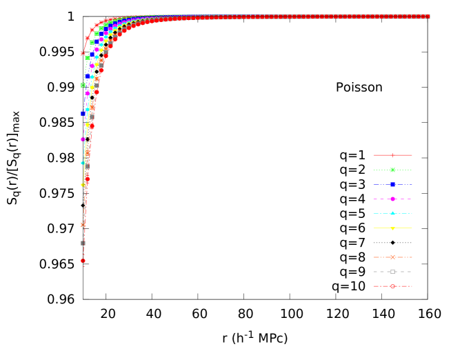
Figure 1: This shows $\frac{S_{q}(r)}{[S_{q}(r)]_{max}}$ as a function of length scale $r$ for a homogeneous Poisson point process. The results for different $q$ values are shown together for a comparison. The $1-\sigma$ errors bars at each data points are obtained from 10 different realizations.

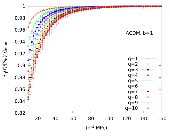
Figure 2: Same as Figure 1 but for unbiased $\Lambda$CDM model.

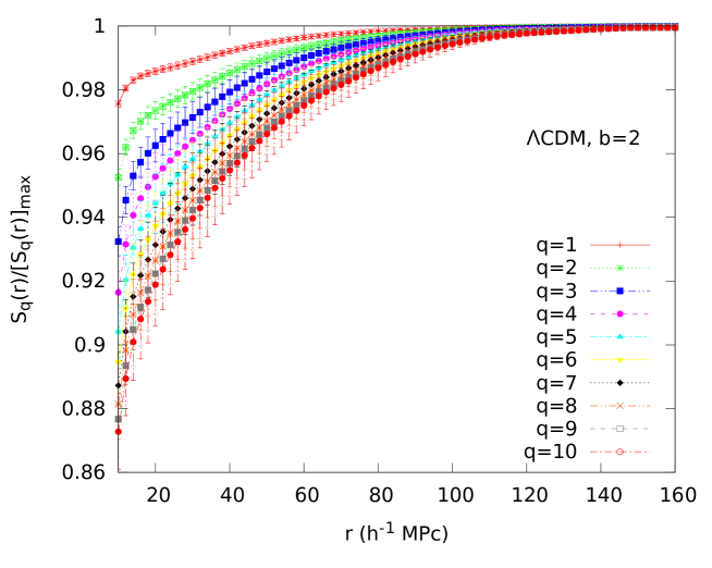
Figure 3: Same as Figure 1 but for $\Lambda$CDM model with $b=2$.

4 Results and Conclusions

We show the Renyi entropies of different order for a homogeneous Poisson point process in Figure 1. The ratio $\frac{S_{q}(r)}{[S_{q}(r)]_{max}}$ for $10$ different $q$ values are shown together as a function of length scale $r$. We see that the ratio deviates from $1$ for all the $q$ values at the smallest length scale $r=10{\,h^{-1}\,{\rm Mpc}}$, the deviation being largest for $q=10$. The larger deviation for higher $q$ values are related to the fact that Renyi entropy is a slowly decreasing function of $q$. The deviations indicate that the distribution is inhomogeneous on $10{\,h^{-1}\,{\rm Mpc}}$. The deviations gradually diminish with increasing radius $r$ for all the $q$ values and the quantity $1-\frac{S_{q}(r)}{[S_{q}(r)]_{max}}$ drops below $10^{-3}$ for all of them on a length scale of $50{\,h^{-1}\,{\rm Mpc}}$. These inhomogeneities are an outcome of the discrete nature of the distributions. All the Poisson distributions analyzed here show a transition to homogeneity on $50{\,h^{-1}\,{\rm Mpc}}$. The $1-\sigma$ errorbars shown at each data point are drawn from 10 different realizations.

We show the results for the unbiased $\Lambda$CDM model in Figure 2. The Figure 2 show a similar trend as observed in Figure 1. However, the degree of inhomogeneities and their variations with length scale in the $\Lambda$CDM model are noticeably different than observed in the Poisson distributions. In this figure, the ratio $\frac{S_{q}(r)}{[S_{q}(r)]_{max}}$ for each values of $q$ shows a larger deviation from 1, as compared to their values observed in Poisson distributions. Further, the inhomogeneities in the $\Lambda$CDM model decrease much slowly with radius $r$ as compared to Poisson distributions. The higher degree of inhomogeneities and their slower variations in the $\Lambda$CDM model arise due to the existence of real inhomogeneities in the distribution. We find that $\frac{S_{q}(r)}{[S_{q}(r)]_{max}}$ for all the $q$ values converges to 1 within $10^{-3}$ at a length scale of $120{\,h^{-1}\,{\rm Mpc}}$. The results indicate a transition to homogeneity at $120{\,h^{-1}\,{\rm Mpc}}$ for the $\Lambda$CDM model. The $1-\sigma$ errorbars at each data point are obtained from 9 different realizations.

We repeat our analysis with the data from the $\Lambda$CDM model with $b=2$ and show the corresponding results in Figure 3. We find that the observed inhomogeneities in the biased $\Lambda$CDM model also diminish with increasing length scales. Interestingly, the degree of inhomogeneities in the biased $\Lambda$CDM model are lower than the unbiased $\Lambda$CDM model for all $q$ values at smaller length scales. However, the inhomogeneities in the biased $\Lambda$CDM model are larger than its unbiased counterpart on larger length scales. The matter distribution is known to exhibit a weblike network of nodes, filaments and sheets surrounded by voids. A biased distribution is primarily composed of particles preferentially identified from rarer density peaks which represent similar environments. So there will be less disparity in the number counts around the centres located in such environments. This is particularly true on smaller length scales up to the physical extent of these regions. But the measurements around these centres would show a larger disparity beyond the extent of these environments On the other hand, the particles are distributed across diverse environments in the unbiased $\Lambda$CDM model. The measuring spheres centred on the particles in such a distribution trace diverse environments giving rise to a larger disparity in their measurements. The disparity in these measurements gradually decrease with increasing length scales until the measuring spheres include statistically similar number of nodes, filaments, sheets and voids. Figure 3 shows that the biased $\Lambda$CDM model show a slower variation of inhomogeneities with length scales than the unbiased model. Consequently, the inhomogeneities extend to a larger length scales in the biased model. We find that the quantity $\frac{S_{q}(r)}{[S_{q}(r)]_{max}}$ for all the $q$ values in the $\Lambda$CDM model with $b=2$ converges to 1 within $10^{-3}$ at a length scale of $140{\,h^{-1}\,{\rm Mpc}}$. We obtain the $1-\sigma$ errorbars at each data point using 10 different realizations.

One particular disadvantage of any number count based method is that the measuring centres progressively get confined towards the centre of the survey volume with increasing length scales. This confinement bias [50, 57] enforces overlaps between the measuring spheres leading towards an apparent homogeneity in any inhomogeneous distributions. The effects of confinement bias can be minimized by increasing the survey volume. However larger survey volume requires us to take in to account the evolution with look back time. This could make anti-Copernican void models to appear homogeneous on larger length scales. Fortunately, other observations like SNe, CMB and BAO can be used to constrain such models [58, 59, 60, 61].

The method proposed in this work has some similarities to the other studies on homogeneity that are based on multifractal analysis [35, 37, 38]. Both of these methods are based on the counts-in-spheres statistics. However, there are some important differences between the two approach. In the multifractal analysis, the Minkowski-Bouligand dimensions $D_{q}$ are estimated from the logarithmic slope of the generalised correlation integral. The generalized dimension $D_{q}$ is independent of $q$ for a mono fractal but depends on the values of $q$ in a multifractal. A monofractal is regarded as homogeneous when $D_{q}$ becomes equal to the ambient dimension irrespective of the order $q$. The positive values of $q$ assign greater weights to the overdense regions whereas negative values put more weights to the underdense regions. The generalized dimensions $D_{q}$ for $q<0$ are known to be very sensitive to the low density regions in finite datasets [63]. This makes it difficult to distinguish empty space from the space filled with matter at low probability, which may dramatically affect $D_{q}$ for the negative $q$ values. The Renyi entropy based method proposed in this work uses only positive values of $q$ where smaller $q$ values weights the probabilities in a more uniform manner and higher $q$ values puts more weights to higher probabilities. The measurements of the spectrum of generalized dimension requires us to calculate the derivative of the generalized correlation integral whereas the present method does not involve any numerical derivatives and hence bypasses the associated errors. The multifractal analysis determines the homogeneity scale based on the scaling of the different moments of galaxy counts, whereas the present method identifies the homogeneity scale based on the maximization of uncertainty in the random variable measuring the density of points. The Renyi entropy is a generalization of the Shannon entropy, which quantify the uncertainty or randomness of a system. The proposed method is based on the simple fact that all the Renyi entropies of different orders must have the same value when the probabilities are equal. We use the normalized Renyi entropies for our analysis which would be less susceptible to the survey geometry and incompleteness effects [40]. On the other hand, the generalized dimension $D_{q}$ is known to be more susceptive to these issues [38, 62].

The cosmological N-body simulations are performed with periodic boundary conditions to mimic the large-scale homogeneity of the matter distribution in the Universe. The periodicity in simulations are typically assumed on the scale of the box. In the present analysis, the simulations were carried out within a comoving volume of $[921.6\,h^{-1}\,{\rm Mpc}]^{3}$ and the scale of homogeneity measured in these simulations lie in the range $120-140\,h^{-1}\,{\rm Mpc}$. These are much smaller than the size of the simulation boxes. We note that the homogeneity scale measured in the homogeneous Poisson distributions are $\sim 50\,h^{-1}\,{\rm Mpc}$ which is significantly smaller than those measured in the unbiased and biased simulations of the $\Lambda$CDM model. Also, the degree of inhomogeneity in the Poisson distributions are reasonably smaller than the distributions derived from the N-body simulations. The Poisson distribution is homogeneous by construction and is expected to exhibit homogeneity on a smaller scale. The small inhomogeneities measured in the Poisson distributions are an outcome of the discreteness noise that diminishes with increasing length scales. Since the measured homogeneity scale in the simulations are significantly smaller than the assumed homogeneity scale, we can accept the measured homogeneity scales as reliable.

We show that the statistical measure proposed in this work can effectively quantify the inhomogeneities present in different types of distributions. The measure can also characterize the nature of inhomogeneities and detect the transition scale to homogeneity, if present in a given distribution. The proposed measure can be used to test the assumption of cosmic homogeneity in the present and future generation galaxy surveys.

References

- [1] T. Buchert, & J. Ehlers, A&A, 320, 1 (1997)
- [2] D. J. Schwarz, arXiv:astro-ph/0209584 (2002)
- [3] E. W. Kolb, S. Matarrese & A. Riotto, New Journal of Physics, 8, 322 (2006)
- [4] T. Buchert, General Relativity and Gravitation, 40, 467 (2008)
- [5] G. F. R. Ellis, Classical and Quantum Gravity, 28, 164001 (2011)
- [6] A. A. Penzias & R. W. Wilson, ApJ, 142, 419 (1965)
- [7] G. F. Smoot, C. L. Bennett, A. Kogut, et al., ApJ Letters, 396, L1 (1992)
- [8] D. J. Fixsen, E. S. Cheng, J. M. Gales, et al., ApJ, 473, 576 (1996)
- [9] R. W. Wilson & A. A. Penzias, Science, 156, 1100 (1967)
- [10] C. Blake & J. Wall, Nature, 416, 150 (2002)
- [11] P. J. E. Peebles, Principles of Physical Cosmology. Princeton, N.J., Princeton University Press (1993)
- [12] K. K. S. Wu, O. Lahav & M. J. Rees, Nature, 397, 225 (1999)
- [13] C. A. Scharf, K. Jahoda, M. Treyer, et al., ApJ, 544, 49 (2000)
- [14] C. A. Meegan, G. J. Fishman, , R. B. Wilson, et al., Nature, 355, 143 (1992)
- [15] M. S. Briggs, W. S. Paciesas, G. N. Pendleton, et al., ApJ, 459, 40 (1996)
- [16] S. Gupta & T. D. Saini, MNRAS, 407, 651 (2010)
- [17] H.-N. Lin, S. Wang, Z. Chang & X.Li,MNRAS, 456, 1881 (2016)
- [18] C. Marinoni, J. Bel & A. Buzzi, JCAP, 10, 036 (2012)
- [19] D. Alonso, A. I. Salvador, F. J. Sánchez, et al., MNRAS, 449, 670 (2015)
- [20] S. Sarkar, B. Pandey, R. Khatri, MNRAS, 483, 2453 (2019)
- [21] L. Pietronero, Physica A Statistical Mechanics and its Applications, 144, 257 (1987)
- [22] P. H. Coleman, L. Pietronero, Physics Reports, 213, 311 (1992)
- [23] B. B. Mandelbrot, Astrophysical Letters and Communications, 36, 1 (1997)
- [24] L. Amendola,& E. Palladino, ApJ Letters, 514, L1 (1999)
- [25] M. Joyce, M. Montuori & F. S. Labini, ApJ Letters, 514, L5 (1999)
- [26] F. Sylos Labini, N. L. Vasilyev & Y. V. Baryshev, A&A, 465, 23 (2007)
- [27] F. Sylos Labini, N. L. Vasilyev & Y. V. Baryshev, A&A, 508, 17 (2009)
- [28] F. Sylos Labini, Europhysics Letters, 96, 59001 (2011)
- [29] V. J. Martinez & P. Coles, ApJ, 437, 550 (1994)
- [30] S. Borgani, Physics Reports, 251, 1 (1995)
- [31] L. Guzzo, New Astronomy, 2, 517 (1997)
- [32] A. Cappi, C. Benoist, L. N. da Costa, & S. Maurogordato, A&A, 335, 779 (1998)
- [33] S. Bharadwaj, A. K. Gupta & T. R. Seshadri, A&A, 351, 405 (1999)
- [34] J. Pan & P. Coles, MNRAS, 318, L51 (2000)
- [35] J. Yadav, S. Bharadwaj, B. Pandey & T. R. Seshadri, MNRAS,364, 601 (2005)
- [36] D. W. Hogg, D. J. Eisenstein, M. R. Blanton, N. A. Bahcall, J. Brinkmann, J. E. Gunn & D. P. Schneider, ApJ, 624, 54 (2005)
- [37] P. Sarkar, J. Yadav, B. Pandey & S. Bharadwaj, MNRAS, 399, L128 (2009)
- [38] M. I. Scrimgeour, T. Davis, C. Blake, et al. 2012, MNRAS, 3412 (2012)
- [39] S. Nadathur, MNRAS, 434, 398 (2013)
- [40] B. Pandey, S. Sarkar, MNRAS, 454, 2647 (2015)
- [41] B. Pandey, S. Sarkar, MNRAS, 460, 1519 (2016)
- [42] J. R., III, Gott, M. Jurić, D. Schlegel, et al., ApJ, 624, 463 (2005)
- [43] R. G. Clowes, K. A. Harris, S. Raghunathan, et al., MNRAS, 429, 2910 (2013)
- [44] I. Szapudi, A. Kovács, B. R. Granett, et al., MNRAS, 450, 288 (2015)
- [45] C. Park, Y.-Y. Choi, J. Kim, J. R. Gott , S. S. Kim , K.-S. Kim, ApJL, 759, L7 (2012)
- [46] V. J. Martinez & B. J. T. Jones, MNRAS, 242, 517 (1990)
- [47] A. Renyi, Probability Theory, Published by North-Holland Publishing Company, Amsterdam (1970)
- [48] H.G.E. Hentschel, I. Procaccia, Physica 8D, 435 (1983)
- [49] W. C. Saslaw, The Distribution of the Galaxies. Published by Cambridge University Press, (1999)
- [50] B. Pandey, MNRAS, 430, 3376 (2013)
- [51] C. E. Shannon, Bell System Technical Journal, 27, 379 (1948)
- [52] S. Sarkar, B. Pandey, MNRAS, 463, L12 (2016)
- [53] D. G. York, et al., AJ, 120, 1579 (2000)
- [54] A. Renyi, Proceedings of the fourth Berkeley Symposium on Mathematics, Statistics and Probability, pp. 547-561 (1961)
- [55] E. Komatsu, et al., ApJS, 180, 330 (2009)
- [56] S. Cole, S. Hatton, D. H. Weinberg, , & C. S. Frenk, MNRAS, 300, 945 (1998)
- [57] D. Kraljic, MNRAS, 451, 3393 (2015)
- [58] J. P. Zibin, A. Moss & D. Scott, Physical Review Letters, 101, 251303 (2008)
- [59] T. Clifton, P. G.Ferreira, , & K. Land, Physical Review Letters, 101, 131302 (2008)
- [60] T. Biswas, A. Notari, & W. Valkenburg, JCAP, 11, 30 (2010)
- [61] C. Clarkson, Comptes Rendus Physique, 13, 682 (2012)
- [62] F. Avila, C. P. Novaes, A. Bernui, E. de Carvalho, J. P. Nogueira-Cavalcante, MNRAS, 488, 1481 (2019)
- [63] A. J. Roberts , 2005, arXiv, nlin/0512014