A Newton Tracking Algorithm with Exact Linear Convergence Rate for Decentralized Consensus Optimization

Abstract

This paper considers the decentralized consensus optimization problem defined over a network where each node holds a second-order differentiable local objective function. Our goal is to minimize the summation of local objective functions and find the exact optimal solution using only local computation and neighboring communication. We propose a novel Newton tracking algorithm, where each node updates its local variable along a local Newton direction modified with neighboring and historical information. We investigate the connections between the proposed Newton tracking algorithm and several existing methods, including gradient tracking and second-order algorithms. Under the strong convexity assumption, we prove that it converges to the exact optimal solution at a linear rate. Numerical experiments demonstrate the efficacy of Newton tracking and validate the theoretical findings.

I INTRODUCTION

In this paper, we focus on the decentralized consensus optimization problem defined over an undirected and connected network with $n$ nodes, in the form of

$${x}^{*}=\arg\min_{x\in\mathbb{R}^{p}}~{}\sum_{i=1}^{n}f_{i}(x).$$ (1)

Here, $f_{i}:\mathbb{R}^{p}\to\mathbb{R}\cup\{+\infty\}$ is a convex and second-order differentiable function privately owned by node $i$. Every agent aims to obtain an optimal solution ${x}^{*}$ to (1) via local computation and communication with its neighbors. Decentralized consensus optimization problem in the form of (1) arises in various applications, such as resource allocation [1, 2, 3], smart grid control [4, 5], federate learning [6, 7, 8], decentralized machine learning [9, 10, 11], and so on.

Decentralized consensus optimization methods have been extensively studied in the literature. Among the first-order methods, a popular algorithm is decentralized gradient descent (DGD) [12, 13, 14]. However, DGD has to employ a diminishing step size to obtain an exact optimal solution. With a fixed step size, DGD converges fast but only to a neighborhood of an optimal solution [14]. There are other first-order methods which use fixed step sizes but still converge to an exact optimal solution, including EXTRA [15], decentralized ADMM [16, 17], exact diffusion [18], NIDS [19], and gradient tracking [20, 21, 22, 23, 24]. Take gradient tracking as an example, each node maintains a local estimate of global gradient descent direction using neighboring and historical information, and uses it to correct the convergence error in DGD.

Although the first-order algorithms enjoy the advantage of low iteration-wise computational complexity, second-order methods are still attractive due to their faster convergence speeds, and hence lower communication costs. Some works such as [25, 26, 27] penalize the implicit consensus constraints to the objective function. Hence, these penalized second-order algorithms can employ unconstrained optimization techniques, but only converge to a neighborhood of an optimal solution. The penalty parameter trade-offs the convergence error and convergence speed. Primal-dual methods are effective to handle this accuracy-speed trade-off. This leads to the second-order methods operating in the primal-dual domain [28, 29, 30], which achieve exact convergence with linear rates. There exist other second-order methods with superlinear convergence rates under stricter conditions [31, 32]. For example, [31] proposes the distributed averaged quasi-Newton method for a master-slave network, but the initialization is required to be close enough to an optimal solution so as to guarantee locally superlinear convergence. The work of [32] runs a finite-time set-consensus inner loop at each iteration of the Polyak’s adaptive Newton method, and achieves globally superlinear convergence.

In this paper, we propose a novel second-order Newton tracking algorithm, in which each node updates its local variable along a local Newton direction modified with neighboring and historical information. As its name suggests, Newton tracking inherits the idea of gradient tracking, but improves its convergence speed through utilizing the second-order information. We investigate the connections between the proposed Newton tracking algorithm and several existing methods, including gradient tracking and second-order algorithms. Under the strong convexity assumption, we prove that it converges to the exact optimal solution at a linear rate. Numerical experiments demonstrate the efficacy of Newton tracking and validate the theoretical findings.

Notations. $\mathbf{I}\in\mathbb{R}^{np\times np}$, $I_{n}\in\mathbb{R}^{n\times n}$ and $I_{p}\in\mathbb{R}^{p\times p}$ denote identity matrices with different sizes. $\mathbf{0}\in\mathbb{R}^{np}$ and $0_{p}\in\mathbb{R}^{p}$ denote all-zero vectors with different sizes. $1_{n}\in\mathbb{R}^{n}$ is an all-one vector. $\lambda_{\max}(\cdot)$, $\lambda_{\min}(\cdot)$ and $\hat{\lambda}_{\min}(\cdot)$ denote the largest, smallest, and smallest nonzero eigenvalues of a matrix, respectively.

II Problem Formulation and Algorithm Development

In this section, we rewrite the decentralized consensus optimization problem (1) to an equivalent constrained form, and propose the Newton tracking algorithm to solve it.

II-A Problem Formulation

Consider a bidirectionally connected network of $n$ nodes. Two nodes are neighbors if they are connected with an edge. Define $\mathcal{N}_{i}$ as the set of neighbors of node $i$ and let ${x}_{i}\in\mathbb{R}^{p}$ be the local copy of decision variable $x$ kept at node $i$. Since the network is bidirectionally connected, the optimization problem in (1) is equivalent to

$$\left\{{x}_{i}^{*}\right\}_{i=1}^{n}:=\underset{\left\{{x}_{i}\right\}_{i=1}^{n}}{{\arg\min}} ~{}\sum_{i=1}^{n}f_{i}\left({x}_{i}\right),$$ (2)

s.t. $$~{}{x}_{i}={x}_{j},~{}\forall j\in\mathcal{N}_{i},~{}\forall i.$$

Indeed, the constraint in (2) enforces the consensus condition ${x}_{1}=\cdots={x}_{n}$ for any feasible solution of (2). When the consensus condition is satisfied, the objective functions in (1) and (2) are equivalent, such that the optimal local variables ${x}_{i}^{*}$ of (2) are all equal to the optimal argument $x^{*}$ of (1), i.e., ${x}_{1}^{*}=\cdots={x}_{n}^{*}=x^{*}$.

II-B Algorithm Development

Let us introduce a nonnegative mixing matrix ${W}\in\mathbb{R}^{n\times n}$ whose $(i,j)$-th element $w_{ij}\geq 0$ represents the weight that node $i$ assigns to node $j$. The weight $w_{ij}=0$ if and only if $j\notin$ $\mathcal{N}_{i}\cup\{i\}$. The mixing matrix $W$ is further required to satisfy the following assumption.

Assumption 1

The mixing matrix $W$ is symmetric and doubly stochastic, i.e., $W=W^{T}$ and $W1_{n}=1_{n}$. The null space of $I_{n}-W$ is $\operatorname{span}\left(1_{n}\right)$.

When the underlying network is bidirectionally connected, the mixing matrix $W$ satisfying Assumption 1 can be generated using various techniques, such as those introduced in [33]. According to the Perron-Frobenius theorem [34], Assumption 1 means that the eigenvalues of $W$ lie in $(-1,1]$ and $W$ has a single eigenvalue at 1.

At time $t$ of our proposed Newton tracking algorithm, each node $i$ keeps a local copy $x_{i}^{t}\in\mathbb{R}^{p}$ and a vector $u_{i}^{t}\in\mathbb{R}^{p}$ that estimates the negative Newton direction $u^{t}$, as

$$u_{i}^{t}\approx u^{t}\triangleq\left(\frac{1}{n}\sum_{i=1}^{n}\nabla^{2}f_{i}(\bar{x}^{t})\right)^{-1}\left(\frac{1}{n}\sum_{i=1}^{n}\nabla f_{i}(\bar{x}^{t})\right),$$

where $\bar{x}^{t}\triangleq\frac{1}{n}\sum_{i=1}^{n}x_{i}^{t}$ is the average of local copies. Each node $i$ updates $x_{i}^{t+1}$ from $x_{i}^{t}$ through descending along the direction $-u_{i}^{t}$ with unit step size. Since it is unaffordable to compute the exact Newton direction in a decentralized manner, we propose to estimate the Newton direction by a novel Newton tracking technique.

To be specific, the proposed Newton tracking algorithm starts with $x_{i}^{0}=0_{p}$ and $u_{i}^{0}=\left(\nabla^{2}f_{i}(0_{p})+\epsilon I_{p}\right)^{-1}\nabla f_{i}(0_{p})$, then proceeds with

$$x_{i}^{t+1}= x_{i}^{t}-u_{i}^{t},$$ (3)

$$u_{i}^{t+1}= (\nabla^{2}f_{i}(x_{i}^{t+1})+\epsilon I_{p})^{-1}$$ (4)

$$\big{[}(\nabla^{2}f_{i}(x_{i}^{t})+\epsilon I_{p})u_{i}^{t}+\nabla f_{i}(x_{i}^{t+1})-\nabla f_{i}(x_{i}^{t})$$

$$+2\alpha(x_{i}^{t+1}-\sum_{j\in\mathcal{N}_{i}}w_{ij}x_{j}^{t+1})-\alpha(x_{i}^{t}-\sum_{j\in\mathcal{N}_{i}}w_{ij}x_{j}^{t})\big{]},$$

where $\epsilon>0$ and $\alpha>0$ are parameters. Comparing $-u_{i}^{t+1}$ with the true Newton direction, we have two observations. (i) The exact global Hessian $\frac{1}{n}\sum_{i=1}^{n}\nabla^{2}f_{i}(\bar{x}^{t+1})$ is replaced by the regularized local Hessian $\nabla^{2}f_{i}(x_{i}^{t+1})+\epsilon I_{p}$. The regularization parameter $\epsilon$ is necessary because the local Hessian $\nabla^{2}f_{i}(x_{i}^{t+1})$ may be unreliable, especially in the beginning stage of the algorithm. (ii) The exact gradient $\frac{1}{n}\sum_{i=1}^{n}\nabla f_{i}(\bar{x}^{t})$ is replaced by three terms that are locally computable. The first term $(\nabla^{2}f_{i}(x_{i}^{t})+\epsilon I_{p})u_{i}^{t}$ involves the previous local Hessian and estimated Newton direction. The second term $\nabla f_{i}(x_{i}^{t+1})-\nabla f_{i}(x_{i}^{t})$ is the difference between the current and previous gradient directions. The third term $2\alpha(x_{i}^{t+1}-\sum_{j\in\mathcal{N}_{i}}w_{ij}x_{j}^{t+1})-\alpha(x_{i}^{t}-\sum_{j\in\mathcal{N}_{i}}w_{ij}x_{j}^{t})$ extrapolates the current and previous consensus errors.

Now we manipulate (4) to better illustrate the idea of Newton tracking. From (4) we have

$$(\nabla^{2}f_{i}(x_{i}^{t+1})+\epsilon I_{p})u_{i}^{t+1}$$ (5)

$$= (\nabla^{2}f_{i}(x_{i}^{t})+\epsilon I_{p})u_{i}^{t}+\nabla f_{i}(x_{i}^{t+1})-\nabla f_{i}(x_{i}^{t})$$

$$+2\alpha(x_{i}^{t+1}-\sum_{j\in\mathcal{N}_{i}}w_{ij}x_{j}^{t+1})-\alpha(x_{i}^{t}-\sum_{j\in\mathcal{N}_{i}}w_{ij}x_{j}^{t}).$$

Summing up (5) over $i=1,\ldots,n$ and invoking the double stochasticity of $W$, we have

$$\sum_{i=1}^{n}\left(\nabla^{2}f_{i}(x_{i}^{t+1})+\epsilon I_{p}\right)u_{i}^{t+1}$$ (6)

$$= \sum_{i=1}^{n}\left(\nabla^{2}f_{i}(x_{i}^{t})+\epsilon I_{p}\right)u_{i}^{t}+\sum_{i=1}^{n}\left(\nabla f_{i}(x_{i}^{t+1})-\nabla f_{i}(x_{i}^{t})\right).$$

When the algorithm is initialized such that $\sum_{i=1}^{n}\nabla f_{i}(x_{i}^{0})$ $=\sum_{i=1}^{n}\left(\nabla^{2}f_{i}(x_{i}^{0})+\epsilon I_{p}\right)u_{i}^{0}$, summing up (6) from time $0$ to time $t$ yields

$$\sum_{i=1}^{n}\left(\nabla^{2}f_{i}(x_{i}^{t})+\epsilon I_{p}\right)u_{i}^{t}=\sum_{i=1}^{n}\nabla f_{i}(x_{i}^{t}).$$

In comparison, the global Newton direction $-u^{t}$ satisfies

$$\sum_{i=1}^{n}\nabla^{2}f_{i}(\bar{x}^{t})u^{t}=\sum_{i=1}^{n}\nabla f_{i}(\bar{x}^{t}).$$

When the local variable pairs $(x_{i}^{t},u_{i}^{t})$ are similar across the nodes, we observe that $x_{i}^{t}$ is close to $\bar{x}^{t}$ and $u_{i}^{t}$ tracks a regularized Newton direction.

The recursion (3)-(4) can be written in a compact form. Define $\mathbf{x}\triangleq[{x}_{1};\ldots;{x}_{n}]\in\mathbb{R}^{np}$ and $\mathbf{u}\triangleq[u_{1};\ldots;u_{n}]\in\mathbb{R}^{np}$ as the stacks of local variables. Define the aggregate function $f:\mathbb{R}^{np}\rightarrow\mathbb{R}$ as $f(\mathbf{x})=f({x}_{1},\cdots,{x}_{n})=\sum_{i=1}^{n}f_{i}({x}_{i})$ that sums up all the local functions $f_{i}\left(x_{i}\right)$. The gradient of $f(\mathbf{x})$ is $\nabla f(\mathbf{x})=[\nabla f_{1}({x}_{1});\ldots;\nabla f_{n}({x}_{n})]\in\mathbb{R}^{np}$. The Hessian of $f(\mathbf{x})$, denoted by $\nabla^{2}f(\mathbf{x})\in\mathbb{R}^{np\times np}$, is a block diagonal matrix whose $i$-th diagonal block is $\nabla^{2}f_{i}(x)$. Define $\mathbf{H}\triangleq\nabla^{2}f(\mathbf{x})+\epsilon\mathbf{I}\in\mathbb{R}^{np\times np}$ and $\mathbf{W}\triangleq{W}\otimes I_{p}\in\mathbb{R}^{np\times np}$ as the Kronecker product of the weight matrix $W$ and the identity matrix $I_{p}$. The recursion (3)-(4) can be written as

$$\mathbf{x}^{t+1}= \mathbf{x}^{t}-\mathbf{u}^{t},$$ (7)

$$\mathbf{u}^{t+1}= ({\mathbf{H}^{t+1}})^{-1}\big{[}\mathbf{H}^{t}\mathbf{u}^{t}+\nabla f\left(\mathbf{x}^{t+1}\right)-\nabla f\left(\mathbf{x}^{t}\right)$$ (8)

$$+\alpha(\mathbf{I}-\mathbf{W})(2\mathbf{x}^{t+1}-\mathbf{x}^{t})\big{]}.$$

The algorithm is initialized as $\mathbf{x}^{0}=\mathbf{0}$ and $\mathbf{u}^{0}=(\nabla^{2}f(\mathbf{0})+\epsilon\mathbf{I})^{-1}\nabla f(\mathbf{0})$.

III Connections with Existing Approaches

This section investigates the connections of the proposed Newton tracking algorithm with several existing approaches, such as gradient tracking and primal-dual methods.

III-A Connection with Gradient Tracking

The recursion of gradient tracking [21] is given by

$$\mathbf{x}^{t+1}=\mathbf{W}\mathbf{x}^{t}-\alpha\mathbf{y}^{t},$$ (9)

$$\mathbf{y}^{t+1}=\mathbf{W}\mathbf{y}^{t}+\nabla{f}(\mathbf{x}^{t+1})-\nabla{f}(\mathbf{x}^{t}),$$ (10)

where $\mathbf{x},\mathbf{y}\in\mathbb{R}^{np}$. To see the connection between gradient tracking and Newton tracking, we rewrite (9)-(10). First, write $\mathbf{x}^{t+1}=\mathbf{W}\mathbf{x}^{t}-\alpha\mathbf{y}^{t}$ as $\mathbf{x}^{t+1}=\mathbf{x}^{t}-[(\mathbf{I}-\mathbf{W})\mathbf{x}^{t}+\alpha\mathbf{y}^{t}]$. Then, define $\mathbf{r}^{t}=(\mathbf{I}-\mathbf{W})\mathbf{x}^{t}+\alpha\mathbf{y}^{t}\in\mathbb{R}^{np}$. Replacing $\mathbf{y}$ with $\mathbf{r}$ shows that (9)-(10) are equivalent to

$$\mathbf{x}^{t+1}= \mathbf{x}^{t}-\mathbf{r}^{t},$$ (11)

$$\mathbf{r}^{t+1}= \mathbf{W}\mathbf{r}^{t}+\alpha[\nabla{f}(\mathbf{x}^{t+1})-\nabla{f}(\mathbf{x}^{t})]$$ (12)

$$+(\mathbf{I}-\mathbf{W})(\mathbf{x}^{t+1}-\mathbf{W}\mathbf{x}^{t}).$$

Similar to the update of $\mathbf{u}^{t+1}$ in (8), the update of $\mathbf{r}^{t+1}$ in (12) also involves three parts: the previous direction $\mathbf{r}^{t}$, the difference between current and previous gradient directions $\alpha[\nabla{f}(\mathbf{x}^{t+1})-\nabla{f}(\mathbf{x}^{t})]$, and the combination of current and previous consensus errors $(\mathbf{I}-\mathbf{W})(\mathbf{x}^{t+1}-\mathbf{W}\mathbf{x}^{t})$. The major difference between $\mathbf{u}^{t+1}$ and $\mathbf{r}^{t+1}$ is that the former utilizes the current and previous Hessians, which help improve the convergence speed, especially when the local objective functions are ill-conditioned.

III-B Connection with Primal-dual Algorithms

The proposed Newton tracking algorithm has a primal-dual interpretation. Note that the null space of $I_{n}-W$ is $\operatorname{span}\left(1_{n}\right)$, so is the null space of its square root $(I_{n}-W)^{\frac{1}{2}}$. Because $(\mathbf{I}-\mathbf{W})^{\frac{1}{2}}=(I_{n}-W)^{\frac{1}{2}}\otimes I_{p}$, $(\mathbf{I}-\mathbf{W})^{\frac{1}{2}}\mathbf{x}=\mathbf{0}$ if and only if $x_{1}=\cdots=x_{n}$. The optimization problem (2) is equivalent to

$$\mathbf{x}^{*}\triangleq\arg\min_{\mathbf{x}} ~{}f(\mathbf{x}),$$ (13)

s.t. $$~{}(\mathbf{I}-\mathbf{W})^{\frac{1}{2}}\mathbf{x}=\mathbf{0}.$$

The augmented Lagrangian $L(\mathbf{x},\mathbf{v})$ of (13) is

$$L(\mathbf{x},\mathbf{v})=f(\mathbf{x})+\langle\mathbf{v},(\mathbf{I}-\mathbf{W})^{\frac{1}{2}}\mathbf{x}\rangle+\frac{\alpha}{2}\mathbf{x}^{T}(\mathbf{I}-\mathbf{W})\mathbf{x},$$ (14)

where $\mathbf{v}\in\mathbb{R}^{np}$ is the dual variable. Therefore, the augmented Lagrangian method to solve (13) is given by

$$\mathbf{x}^{t+1} =\arg\min_{\mathbf{x}}~{}L(\mathbf{x},\mathbf{v}^{k}),$$ (15)

$$\mathbf{v}^{t+1} =\mathbf{v}^{t}+\alpha(\mathbf{I}-\mathbf{W})^{\frac{1}{2}}\mathbf{x}^{t+1}.$$ (16)

However, solving (15) is nontrivial. First, $f(\mathbf{x})$ is a general objective function such that (15) does not have a closed-form solution. Second, even if $f(\mathbf{x})$ is quadratic, the topology-dependent quadratic term $\frac{\alpha}{2}\mathbf{x}^{T}(\mathbf{I}-\mathbf{W})\mathbf{x}$ makes the closed-form solution not implementable in a decentralized manner. Motivated by these observations, we quadratically approximate $f(\mathbf{x})$ and linearly approximate $\frac{\alpha}{2}\mathbf{x}^{T}(\mathbf{I}-\mathbf{W})\mathbf{x}$ both around $\mathbf{x}^{t}$, and then add a proximal term $\frac{\epsilon}{2}\|\mathbf{x}-\mathbf{x}^{t}\|^{2}$ to the objective function of (15). This way, the update of $\mathbf{x}^{t+1}$ is given by the solution to

$$\min_{\mathbf{x}} ~{}\left\langle\triangledown f(\mathbf{x}^{t})\!+\!(\mathbf{I}-\mathbf{W})^{\frac{1}{2}}\mathbf{v}^{t}+\alpha(\mathbf{I}-\mathbf{W})\mathbf{x}^{t},\mathbf{x}-\mathbf{x}^{t}\!\right\rangle$$

$$~{}+\frac{1}{2}(\mathbf{x}-\mathbf{x}^{t})^{T}\triangledown^{2}f(\mathbf{x}^{t})(\mathbf{x}-\mathbf{x}^{t})+\frac{\epsilon}{2}\|\mathbf{x}-\mathbf{x}^{t}\|^{2},$$

which is

$$\mathbf{x}^{t+1}=\mathbf{x}^{t}$$ (17)

$$\hskip 10.00002pt-\left(\mathbf{H}^{t}\right)^{-1}\left[\nabla f\left(\mathbf{x}^{t}\right)+(\mathbf{I}-\mathbf{W})^{\frac{1}{2}}\mathbf{v}^{t}+\alpha(\mathbf{I}-\mathbf{W})\mathbf{x}^{t}\right].$$

Next, we show that (17) and (16) initialized by $\mathbf{x}^{0}=\mathbf{0}$ and $\mathbf{v}^{0}=\mathbf{0}$ are equivalent to (7)-(8) initialized by $\mathbf{x}^{0}=\mathbf{0}$ and $\mathbf{u}^{0}=(\nabla^{2}f(\mathbf{0})+\epsilon\mathbf{I})^{-1}\nabla f(\mathbf{0})$. By (17), the two recursions have the same $\mathbf{x}^{1}=-(\nabla^{2}f(\mathbf{0})+\epsilon\mathbf{I})^{-1}\nabla f(\mathbf{0})$. Also by (17), we have

$$\mathbf{H}^{t}\mathbf{x}^{t+1}=\mathbf{H}^{t}\mathbf{x}^{t}$$ (18)

$$\hskip 10.00002pt-\left[\nabla f\left(\mathbf{x}^{t}\right)+(\mathbf{I}-\mathbf{W})^{\frac{1}{2}}\mathbf{v}^{t}+\alpha(\mathbf{I}-\mathbf{W})\mathbf{x}^{t}\right],$$

$$\mathbf{H}^{t+1}\mathbf{x}^{t+2}=\mathbf{H}^{t+1}\mathbf{x}^{t+1}$$ (19)

$$\hskip 10.00002pt-\left[\nabla f\left(\mathbf{x}^{t+1}\right)+(\mathbf{I}-\mathbf{W})^{\frac{1}{2}}\mathbf{v}^{t+1}+\alpha(\mathbf{I}-\mathbf{W})\mathbf{x}^{t+1}\right],$$

Subtracting (18) from (19) and substituting the dual update (16) to eliminate the terms $(\mathbf{I}-\mathbf{W})^{\frac{1}{2}}\mathbf{v}^{t}$ and $(\mathbf{I}-\mathbf{W})^{\frac{1}{2}}\mathbf{v}^{t+1}$, we have

$$\mathbf{H}^{t+1}\mathbf{x}^{t+2}=\left[\mathbf{H}^{t}+\mathbf{H}^{t+1}-2\alpha(\mathbf{I}-\mathbf{W})\right]\mathbf{x}^{t+1}$$

$$-\left[\mathbf{H}^{t}-\alpha(\mathbf{I}-\mathbf{W})\right]\mathbf{x}^{t}-\left[\nabla f\left(\mathbf{x}^{t+1}\right)-\nabla f\left(\mathbf{x}^{t}\right)\right],$$

which is equivalent to

$$\mathbf{H}^{t+1}\mathbf{x}^{t+2}-\left[\mathbf{H}^{t+1}-\alpha(\mathbf{I}-\mathbf{W})\right]\mathbf{x}^{t+1}$$ (20)

$$= \mathbf{H}^{t}\mathbf{x}^{t+1}-\left[\mathbf{H}^{t}-\alpha(\mathbf{I}-\mathbf{W})\right]\mathbf{x}^{t}-\alpha(\mathbf{I}-\mathbf{W})\mathbf{x}^{t+1}$$

$$-\left[\nabla f\left(\mathbf{x}^{t+1}\right)-\nabla f\left(\mathbf{x}^{t}\right)\right].$$

Defining $\mathbf{s}^{t}\triangleq\mathbf{H}^{t}\mathbf{x}^{t+1}-\left[\mathbf{H}^{t}-\alpha(\mathbf{I}-\mathbf{W})\right]\mathbf{x}^{t}$, we rewrite (20) as

$$\mathbf{s}^{t+1}= \mathbf{s}^{t}-\alpha(\mathbf{I}-\mathbf{W})\mathbf{x}^{t+1}-\left[\nabla f\left(\mathbf{x}^{t+1}\right)-\nabla f\left(\mathbf{x}^{t}\right)\right].$$ (21)

From the definition of $\mathbf{s}^{t}$, it holds

$$\mathbf{x}^{t+1} =\mathbf{x}^{t}-({\mathbf{H}^{t}})^{-1}\left[\alpha(\mathbf{I}-\mathbf{W})\mathbf{x}^{t}-\mathbf{s}^{t}\right].$$ (22)

Further defining $\mathbf{q}^{t}\triangleq\alpha(\mathbf{I}-\mathbf{W})\mathbf{x}^{t}-\mathbf{s}^{t}=\mathbf{H}^{t}(\mathbf{x}^{t}-\mathbf{x}^{t+1})$, we rewrite (22) and (21) as

$$\mathbf{x}^{t+1}= \mathbf{x}^{t}-({\mathbf{H}^{t}})^{-1}\mathbf{q}^{t},$$ (23)

$$\mathbf{q}^{t+1}= \mathbf{q}^{t}+\nabla f\left(\mathbf{x}^{t+1}\right)-\nabla f\left(\mathbf{x}^{t}\right)$$ (24)

$$+\alpha(\mathbf{I}-\mathbf{W})(2\mathbf{x}^{t+1}-\mathbf{x}^{t}).$$

Observe that (23)-(24) are equivalent to (7)-(8) in the sense of $\mathbf{u}^{t}=({\mathbf{H}^{t}})^{-1}\mathbf{q}^{t}$.

Remark 1

There is an existing primal-dual second-order algorithm called ESOM that also quadratically approximates the augmented Lagrangian when solving (15) [29]. However, unlike the proposed Newton tracking algorithm, ESOM does not linearize the topology-dependent quadratic term $\frac{\alpha}{2}\mathbf{x}^{T}(\mathbf{I}-\mathbf{W})\mathbf{x}$, which, as we have indicated earlier, makes the closed-form solution not implementable in a decentralized manner. In fact, the primal update of ESOM is given by

$$\mathbf{x}^{t+1}= \mathbf{x}^{t}-\left(\triangledown^{2}f(\mathbf{x})+\alpha(\mathbf{I}-\mathbf{W})+\epsilon\mathbf{I}\right)^{-1}$$ (25)

$$\big{[}\nabla f\left(\mathbf{x}^{t}\right)+(\mathbf{I}-\mathbf{W})^{\frac{1}{2}}\mathbf{v}^{t}+\alpha(\mathbf{I}-\mathbf{W})\mathbf{x}^{t}\big{]}.$$

In (25), computing the inverse of $\triangledown^{2}f(\mathbf{x})+\alpha(\mathbf{I}-\mathbf{W})+\epsilon\mathbf{I}$ requires multiple rounds of communication and computation. Therefore, ESOM introduces an inner loop to approximately solve (25), which leads to extra communication and computation costs [29].

IV convergence analysis

Since the Newton tracking recursion (7)-(8) is equivalent to the primal-dual iteration in (17) and (16), once we show that the primal-dual iteration in (17) and (16) exhibits a linear convergence rate, then so does the Newton tracking recursion (7)-(8). In the analysis, we need the following assumption.

Assumption 2

The local objective functions $f_{i}(x_{i})$ are twice differentiable. The eigenvalues of Hessians $\nabla^{2}f_{i}(x_{i})$ are bounded by positive constants $\mu_{f},L_{f}\in(0,\infty)$, i.e.

$$\mu_{f}I_{p}\preceq\nabla^{2}f_{i}\left(x_{i}\right)\preceq L_{f}I_{p},$$ (26)

for all $x_{i}\in\mathbb{R}^{p}$ and $i=1,\ldots,n$.

The lower bound in (26) implies that the local objective functions $f_{i}(x)$ are strongly convex with constant $\mu_{f}>0$. The upper bound implies that the local gradients $\nabla f_{i}(x)$ are Lipschitz continuous with constant $L_{f}$. Note that the aggregate objective function $\nabla^{2}f(\mathbf{x})$ is a block diagonal matrix whose $i$-th diagonal block is $\nabla^{2}f_{i}(x)$. Therefore, the bounds on the eigenvalues of Hessians $\nabla^{2}f_{i}(x)$ in (26) also hold for the aggregate Hessian, i.e.

$$\mu_{f}\mathbf{I}\preceq\nabla^{2}f(\mathbf{x})\preceq L_{f}\mathbf{I},$$

for all $\mathbf{x}\in\mathbb{R}^{np}$. Thus, the aggregate objective function $f(\mathbf{x})$ is also strongly convex with constant $\mu_{f}$ and its gradients $\nabla f(\mathbf{x})$ are Lipschitz continuous with constant $L_{f}$.

Our analysis involves the optimal primal-dual pair $(\mathbf{x}^{*},\mathbf{v}^{*})$ of (13). According to the KKT condition of (13), we have

$$\triangledown f(\mathbf{x}^{*})+(\mathbf{I}-\mathbf{W})^{\frac{1}{2}}\mathbf{v}^{*}=\mathbf{0},$$ (27)

$$(\mathbf{I}-\mathbf{W})^{\frac{1}{2}}\mathbf{x}^{*}=0\quad\text{or}\quad(\mathbf{I}-\mathbf{W})\mathbf{x}^{*}=\mathbf{0}.$$ (28)

Lemma 1

Consider the equivalent Newton tracking iteration in (17) and (16). The primal-dual iterate satisfies

$$\nabla f\left(\mathbf{x}^{t+1}\right) -\nabla f\left(\mathbf{x}^{*}\right)+(\mathbf{I}-\mathbf{W})^{\frac{1}{2}}\left(\mathbf{v}^{t+1}-\mathbf{v}^{*}\right)$$ (29)

$$+\epsilon\left(\mathbf{x}^{t+1}-\mathbf{x}^{t}\right)+\mathbf{e}^{t}=\mathbf{0},$$

where $\mathbf{e}^{t}$ is defined as

$$\mathbf{e}^{t}\triangleq \nabla f\left(\mathbf{x}^{t}\right)-\nabla f\left(\mathbf{x}^{t+1}\right)+\nabla^{2}f\left(\mathbf{x}^{t}\right)\left(\mathbf{x}^{t+1}-\mathbf{x}^{t}\right)$$ (30)

$$-\alpha(\mathbf{I}-\mathbf{W})(\mathbf{x}^{t+1}-\mathbf{x}^{t}).$$

The result in Lemma 1 shows the relationship of the primal-dual pairs $(\mathbf{x}^{t},\mathbf{v}^{t})$ and $(\mathbf{x}^{t+1},\mathbf{v}^{t+1})$ with the optimal primal-dual pair $(\mathbf{x}^{*},\mathbf{v}^{*})$. The arguments used in the proof of Lemma 1 are similar to ones used in [29].

Proof 1

By the definition of $\mathbf{e}^{t}$, (17) can be rewritten as

$${\nabla f\left(\mathbf{x}^{t+1}\right)+(\mathbf{I}-\mathbf{W})^{\frac{1}{2}}\mathbf{v}^{t}}+\alpha(\mathbf{I}-{\mathbf{W}})\mathbf{x}^{t+1}$$ (31)

$$\quad+\epsilon\left(\mathbf{x}^{t+1}-\mathbf{x}^{t}\right)+\mathbf{e}^{t}=\mathbf{0}.$$

Combining (27) and (28) with (31), we have

$${\nabla f\left(\mathbf{x}^{t+1}\right)-\nabla f\left(\mathbf{x}^{*}\right)+(\mathbf{I}-\mathbf{W})^{\frac{1}{2}}\left(\mathbf{v}^{t}-\mathbf{v}^{*}\right)}$$ (32)

$$\quad+\alpha(\mathbf{I}-\mathbf{W})\left(\mathbf{x}^{t+1}-\mathbf{x}^{*}\right)+\epsilon\left(\mathbf{x}^{t+1}-\mathbf{x}^{t}\right)+\mathbf{e}^{t}=\mathbf{0}.$$

Observe that $\mathbf{v}^{t}$ in (32) can be further replaced by $\mathbf{v}^{t+1}$. To be specific, substituting (28) into (16) and then regrouping terms, we know that $\mathbf{v}^{t}$ can be represented as

$$\mathbf{v}^{t}=\mathbf{v}^{t+1}-\alpha(\mathbf{I}-\mathbf{W})^{\frac{1}{2}}\left(\mathbf{x}^{t+1}-\mathbf{x}^{*}\right).$$ (33)

Substituting (33) into (32) yields (29).

Observe that the term $\mathbf{e}^{t}$ can be interpreted as the error introduced by approximation at time $t$, which motivates us to find an upper bound for $\|\mathbf{e}^{t}\|$. In the following lemma, we provide an upper bound for $\left\|\mathbf{e}^{t}\right\|$ in terms of $\left\|\mathbf{x}^{t+1}-\mathbf{x}^{t}\right\|$.

Lemma 2

Consider the equivalent Newton tracking iteration in (17) and (16), and recall the definition of the error vector $\mathbf{e}^{t}$ in (30). If Assumption 2 holds, then $\|\mathbf{e}^{t}\|$ is bounded by

$$\left\|\mathbf{e}^{t}\right\|\leq\kappa\left\|\mathbf{x}^{t+1}-\mathbf{x}^{t}\right\|.$$ (34)

where $\kappa\triangleq 2L_{f}+\alpha\lambda_{\max}(\mathbf{I}-\mathbf{W})$.

Proof 2

By the triangle inequality, $\|\mathbf{e}^{t}\|$ is bounded by

$$\|\mathbf{e}^{t}\|\leq\|\nabla f\left(\mathbf{x}^{t}\right)-\nabla f\left(\mathbf{x}^{t+1}\right)\|$$ (35)

$$+\|\nabla^{2}f\left(\mathbf{x}^{t}\right)\left(\mathbf{x}^{t+1}-\mathbf{x}^{t}\right)\|+\|\alpha(\mathbf{I}-\mathbf{W})(\mathbf{x}^{t+1}-\mathbf{x}^{t})\|.$$

By Assumption 2, $\|\nabla f\left(\mathbf{x}^{t}\right)-\nabla f\left(\mathbf{x}^{t+1}\right)\|\leq L_{f}\|\mathbf{x}^{t+1}-\mathbf{x}^{t}\|$. As the largest eigenvalue of $\nabla^{2}f\left(\mathbf{x}^{t}\right)$ and $\mathbf{I}-\mathbf{W}$ are $L_{f}$ and $\lambda_{\max}(\mathbf{I}-\mathbf{W})$, respectively, we know $\|\nabla^{2}f\left(\mathbf{x}^{t}\right)\left(\mathbf{x}^{t+1}\right.$ $\left.-\mathbf{x}^{t}\right)\|\leq L_{f}\|\mathbf{x}^{t+1}-\mathbf{x}^{t}\|$ and $\|\alpha(\mathbf{I}-\mathbf{W})(\mathbf{x}^{t+1}-\mathbf{x}^{t})\|\leq\lambda_{\max}(\mathbf{I}-\mathbf{W})\|\mathbf{x}^{t+1}-\mathbf{x}^{t}\|$. Substituting these inequalities into (35) completes the proof.

The result in (34) demonstrates that the error $\mathbf{e}^{t}$ introduced by approximation becomes zero as the sequence of iterates $\mathbf{x}^{t}$ approaches the optimal solution $\mathbf{x}^{*}$, which will be shown in Theorem 1.

Given the preliminary results in Lemmas 1 and 2, we are ready to establish the linear convergence of the proposed Newton tracking method. To do so, we define vectors $\mathbf{\zeta},\mathbf{\zeta}^{*}\in\mathbb{R}^{2np}$ and a matrix $\mathbf{G}\in\mathbb{R}^{np\times np}$ as

$$\mathbf{\zeta}^{t}=\left[\begin{array}[]{l}{\mathbf{x}^{t}}\\ {\mathbf{v}^{t}}\end{array}\right],~{}\mathbf{\zeta}^{*}=\left[\begin{array}[]{l}{\mathbf{x}^{*}}\\ {\mathbf{v}^{*}}\end{array}\right],~{}\mathbf{G}=\left[\begin{array}[]{cc}\mathbf{Q}&\mathbf{0}\\ \mathbf{0}&{\frac{1}{\alpha}\mathbf{I}}\end{array}\right],$$

where $\mathbf{Q}\triangleq\epsilon\mathbf{I}-\alpha(\mathbf{I}-\mathbf{W})$. Note that $\mathbf{Q}$ is positive definite when $\epsilon-\alpha\lambda_{\max}(\mathbf{I}-\mathbf{W})>0$. In the following theorem, we show that the sequence $\|\mathbf{\zeta}^{t}-\mathbf{\zeta}^{*}\|_{\mathbf{G}}$ converges to zero at a linear rate.

Theorem 1

Consider the equivalent Newton tracking iteration in (17) and (16). Suppose that the parameters $\epsilon$ and $\alpha$ satisfy $\lambda_{\min}(\mathbf{Q})=\epsilon-\alpha\lambda_{\max}(\mathbf{I}-\mathbf{W})>\frac{4L_{f}^{2}}{\mu_{f}}$. Then, the sequence of $\left\|\mathbf{\zeta}^{t}-\mathbf{\zeta}^{*}\right\|_{\mathbf{G}}^{2}$ satisfies

$$\left\|\mathbf{\zeta}^{t+1}-\mathbf{\zeta}^{*}\right\|_{\mathbf{G}}^{2}\leq\frac{1}{1+{\delta}^{\prime}}\left\|\mathbf{\zeta}^{t}-\mathbf{\zeta}^{*}\right\|_{\mathbf{G}}^{2},$$ (36)

where

$${\delta}^{\prime}= \min\left\{\frac{\mu_{f}\delta}{(1+\delta)\left[\epsilon+\frac{\beta\phi L_{f}^{2}}{{\alpha\hat{\lambda}_{\min}(\mathbf{I}-\mathbf{W})}}\right]},\right.$$

$$\left.\frac{\alpha\delta^{2}(\epsilon-\alpha\lambda_{\max}(\mathbf{I}-\mathbf{W})){\hat{\lambda}_{\min}(\mathbf{I}-\mathbf{W})}}{\frac{\beta\epsilon^{2}}{(\beta-1)}+\frac{\beta\phi(2L_{f}+\alpha\lambda_{\max}(\mathbf{I}-\mathbf{W}))^{2}}{(\phi-1)}}\right\}.$$ (37)

Therein, $\beta>1$ and $\phi>1$ are arbitrary constants, and

$$\delta\triangleq 1-\frac{4L_{f}^{2}}{\mu_{f}{\lambda_{\min}({\mathbf{Q}})}}=1-\frac{4L_{f}^{2}}{\mu_{f}(\epsilon-\alpha\lambda_{\max}(\mathbf{I}-\mathbf{W}))}>0.$$

Proof 3

Step 1. By reorganizing (17), we get

$$\epsilon(\mathbf{x}^{t}-\mathbf{x}^{t+1})+\triangledown^{2}f(\mathbf{x}^{t})\left(\mathbf{x}^{t}-\mathbf{x}^{t+1}\right)$$

$$-\left[\nabla f\left(\mathbf{x}^{t}\right)+(\mathbf{I}-\mathbf{W})^{\frac{1}{2}}\mathbf{v}^{t}+\alpha(\mathbf{I}-\mathbf{W})\mathbf{x}^{t}\right]=\mathbf{0}.$$

Thus, it holds

$$\left\langle\mathbf{x}^{*}-\mathbf{x}^{t+1},\epsilon(\mathbf{x}^{t}-\mathbf{x}^{t+1})+\triangledown^{2}f(\mathbf{x}^{t})\left(\mathbf{x}^{t}-\mathbf{x}^{t+1}\right)\right.$$ (38)

$$\left.-\left[\nabla f\left(\mathbf{x}^{t}\right)+(\mathbf{I}-\mathbf{W})^{\frac{1}{2}}\mathbf{v}^{t}+\alpha(\mathbf{I}-\mathbf{W})\mathbf{x}^{t}\right]\right\rangle={0}.$$

Substituting the dual update $\mathbf{v}^{t}=\mathbf{v}^{t+1}-\alpha(\mathbf{I}-\mathbf{W})^{\frac{1}{2}}\mathbf{x}^{t+1}$ and regrouping the terms, we can rewrite (38) to

$$\left\langle\mathbf{x}^{*}-\mathbf{x}^{t+1},\underbrace{\left(\epsilon\mathbf{I}-\alpha(\mathbf{I}-\mathbf{W})\right)}_{\triangleq\mathbf{Q}}(\mathbf{x}^{t}-\mathbf{x}^{t+1})\right\rangle$$ (39)

$$-\left\langle\mathbf{x}^{*}-\mathbf{x}^{t+1},\nabla f\left(\mathbf{x}^{t}\right)\right\rangle-\left\langle\mathbf{x}^{*}-\mathbf{x}^{t+1},(\mathbf{I}-\mathbf{W})^{\frac{1}{2}}\mathbf{v}^{t+1}\right\rangle$$

$$+\left\langle\mathbf{x}^{*}-\mathbf{x}^{t+1},\triangledown^{2}f(\mathbf{x}^{t})(\mathbf{x}^{t}-\mathbf{x}^{t+1})\right\rangle={0}.$$

For the first term at the left-hand side of (39), we have

$$\left\langle\mathbf{x}^{*}-\mathbf{x}^{t+1},\mathbf{Q}(\mathbf{x}^{t}-\mathbf{x}^{t+1})\right\rangle$$ (40)

$$= \frac{1}{2}\big{(}\|\mathbf{x}^{*}-\mathbf{x}^{t+1}\|_{\mathbf{Q}}^{2}+\|\mathbf{x}^{t}-\mathbf{x}^{t+1}\|_{\mathbf{Q}}^{2}-\|\mathbf{x}^{*}-\mathbf{x}^{t}\|_{\mathbf{Q}}^{2}\big{)}.$$

For the second term at the left-hand side of (39), according to the $\mu_{f}$-strong convexity of $f$, we have

$$\left\langle\mathbf{x}^{*}-\mathbf{x}^{t+1},\nabla f\left(\mathbf{x}^{t}\right)\right\rangle$$ (41)

$$= \left\langle\mathbf{x}^{*}-\mathbf{x}^{t+1},\nabla f\left(\mathbf{x}^{t+1}\right)\right\rangle$$

$$+\left\langle\mathbf{x}^{*}-\mathbf{x}^{t+1},\nabla f\left(\mathbf{x}^{t}\right)-\nabla f\left(\mathbf{x}^{t+1}\right)\right\rangle$$

$$\leq f(\mathbf{x}^{*})-f\left(\mathbf{x}^{t+1}\right)-\frac{\mu_{f}}{2}\left\|\mathbf{x}^{*}-\mathbf{x}^{t+1}\right\|^{2}$$

$$+\left\langle\mathbf{x}^{*}-\mathbf{x}^{t+1},\nabla f\left(\mathbf{x}^{t}\right)-\nabla f\left(\mathbf{x}^{t+1}\right)\right\rangle.$$

Substituting (41) and (40) into (39), we get

$$\frac{1}{2}\big{(}\|\mathbf{x}^{*}-\mathbf{x}^{t+1}\|_{\mathbf{Q}}^{2}+\|\mathbf{x}^{t}-\mathbf{x}^{t+1}\|_{\mathbf{Q}}^{2}-\|\mathbf{x}^{*}-\mathbf{x}^{t}\|_{\mathbf{Q}}^{2}\big{)}$$ (42)

$$- f(\mathbf{x}^{*})+f\left(\mathbf{x}^{t+1}\right)+\frac{\mu_{f}}{2}\left\|\mathbf{x}^{*}-\mathbf{x}^{t+1}\right\|^{2}$$

$$+ \left\langle\mathbf{x}^{*}-\mathbf{x}^{t+1},\nabla f\left(\mathbf{x}^{t+1}\right)-\nabla f\left(\mathbf{x}^{t}\right)+\triangledown^{2}f(\mathbf{x}^{t})(\mathbf{x}^{t}-\mathbf{x}^{t+1})\right\rangle$$

$$- \left\langle\mathbf{x}^{*}-\mathbf{x}^{t+1},(\mathbf{I}-\mathbf{W})^{\frac{1}{2}}\mathbf{v}^{t+1}\right\rangle\leq 0.$$

After being regrouped, (42) becomes

$$\underbrace{f(\mathbf{x}^{*})-f\left(\mathbf{x}^{t+1}\right)}_{(i)}+\underbrace{\left\langle\mathbf{x}^{*}-\mathbf{x}^{t+1},(\mathbf{I}-\mathbf{W})^{\frac{1}{2}}\mathbf{v}^{t+1}\right\rangle}_{(ii)}$$ (43)

$$-\frac{1}{2}\big{(}\|\mathbf{x}^{*}-\mathbf{x}^{t+1}\|_{\mathbf{Q}}^{2}-\|\mathbf{x}^{*}-\mathbf{x}^{t}\|_{\mathbf{Q}}^{2}\big{)}$$

$$\geq \frac{1}{2}\|\mathbf{x}^{t}-\mathbf{x}^{t+1}\|_{\mathbf{Q}}^{2}+\frac{\mu_{f}}{2}\left\|\mathbf{x}^{*}-\mathbf{x}^{t+1}\right\|^{2}$$

$$+ \left\langle\mathbf{x}^{*}-\mathbf{x}^{t+1},\nabla f\left(\mathbf{x}^{t+1}\right)-\nabla f\left(\mathbf{x}^{t}\right)+\triangledown^{2}f(\mathbf{x}^{t})(\mathbf{x}^{t}-\mathbf{x}^{t+1})\right\rangle.$$

Step 2. We proceed to simplify (43). According to the dual update (16), $\mathbf{v}^{t+1}=\mathbf{v}^{t}+\alpha(\mathbf{I}-\mathbf{W})^{\frac{1}{2}}\mathbf{x}^{t+1}$ and consequently

$$\big{\langle}{\mathbf{v}^{*}}-{\mathbf{v}^{t+1}},-(\mathbf{I}-\mathbf{W})^{\frac{1}{2}}\mathbf{x}^{t+1}\big{\rangle}$$

$$= \left\langle\mathbf{v}^{*}-\mathbf{v}^{t+1},\frac{\mathbf{v}^{t}-\mathbf{v}^{t+1}}{\alpha}\right\rangle$$

$$= \frac{1}{2\alpha}\left(\|\mathbf{v}^{t+1}-\mathbf{v}^{t}\|^{2}-\|\mathbf{v}^{*}-\mathbf{v}^{t}\|^{2}+\|\mathbf{v}^{*}-\mathbf{v}^{t+1}\|^{2}\right).$$

Reorganizing the terms, we have

$$\underbrace{\big{\langle}{\mathbf{v}^{*}},-(\mathbf{I}-\mathbf{W})^{\frac{1}{2}}\mathbf{x}^{t+1}\big{\rangle}}_{(i^{\prime})}+\underbrace{\big{\langle}{\mathbf{v}^{t+1}},(\mathbf{I}-\mathbf{W})^{\frac{1}{2}}\mathbf{x}^{t+1}\big{\rangle}}_{(ii^{\prime})}$$ (44)

$$+\frac{1}{2\alpha}\left(\|\mathbf{v}^{*}-\mathbf{v}^{t}\|^{2}-\|\mathbf{v}^{*}-\mathbf{v}^{t+1}\|^{2}\right)$$

$$= \frac{1}{2\alpha}\|\mathbf{v}^{t+1}-\mathbf{v}^{t}\|^{2}.$$

Next, we sum up (43) and (44). The summation of $(i)$ and $(i^{\prime})$ can be simplified as

$$f(\mathbf{x}^{*})-f(\mathbf{x}^{t+1})+\big{\langle}\mathbf{v}^{*},-(\mathbf{I}-\mathbf{W})^{\frac{1}{2}}\mathbf{x}^{t+1}\big{\rangle}$$ (45)

$$= \hat{L}(\mathbf{x}^{*},\mathbf{v}^{*})-\hat{L}(\mathbf{x}^{t+1},\mathbf{v}^{*})\leq 0,$$

where $\hat{L}(\mathbf{x},\mathbf{v})=f(\mathbf{x})+\langle\mathbf{v},(\mathbf{I}-\mathbf{W})^{\frac{1}{2}}\mathbf{x}\rangle$ is the Lagrangian of (13). The inequality holds because $(\mathbf{x}^{*},\mathbf{v}^{*})$ is the saddle point of $\hat{L}(\mathbf{x},\mathbf{v})$. The summation of $(ii)$ and $(ii^{\prime})$ is

$$\big{\langle}\mathbf{x}^{*}-\mathbf{x}^{t+1},(\mathbf{I}-\mathbf{W})^{\frac{1}{2}}\mathbf{v}^{t+1}\big{\rangle}+\big{\langle}\mathbf{v}^{t+1},(\mathbf{I}-\mathbf{W})^{\frac{1}{2}}\mathbf{x}^{t+1}\big{\rangle}$$

$$= \big{\langle}\mathbf{x}^{*},(\mathbf{I}-\mathbf{W})^{\frac{1}{2}}\mathbf{v}^{t+1}\big{\rangle}=0.$$ (46)

Note that in deriving both (45) and (3), we utilize the consensus condition $(\mathbf{I}-\mathbf{W})^{\frac{1}{2}}\mathbf{x}^{*}=\mathbf{0}$. With (45) and (3), the summation of (43) and (44) is

$$\frac{1}{2}\left(\|\mathbf{x}^{*}\!-\!\mathbf{x}^{t}\|_{\mathbf{Q}}^{2}-\|\mathbf{x}^{*}\!-\!\mathbf{x}^{t+1}\|_{\mathbf{Q}}^{2}\right)$$ (47)

$$+\frac{1}{2\alpha}\left(\|\mathbf{v}^{*}-\mathbf{v}^{t}\|^{2}-\|\mathbf{v}^{*}-\mathbf{v}^{t+1}\|^{2}\right)$$

$$\geq \frac{1}{2}\|\mathbf{x}^{t}\!-\!\mathbf{x}^{t+1}\|_{\mathbf{Q}}^{2}+\frac{1}{2\alpha}\|\mathbf{v}^{t+1}-\mathbf{v}^{t}\|^{2}+\frac{\mu_{f}}{2}\left\|\mathbf{x}^{*}-\mathbf{x}^{t+1}\right\|^{2}$$

$$+ \left\langle\mathbf{x}^{*}-\mathbf{x}^{t+1},\nabla f\left(\mathbf{x}^{t+1}\right)-\nabla f\left(\mathbf{x}^{t}\right)+\triangledown^{2}f(\mathbf{x}^{t})(\mathbf{x}^{t}-\mathbf{x}^{t+1})\right\rangle.$$

It is the $\mu_{f}$-strong convexity of $f$ that brings the quadratic term $\frac{\mu_{f}}{2}\|\mathbf{x}^{*}-\mathbf{x}^{t+1}\|^{2}$ in (47), which enables us to establish the linear convergence. Indeed, by Cauchy-Schwarz inequality, for any $\theta>0$ we have

$$\left\langle\mathbf{x}^{*}-\mathbf{x}^{t+1},\nabla f\left(\mathbf{x}^{t+1}\right)-\nabla f\left(\mathbf{x}^{t}\right)+\triangledown^{2}f(\mathbf{x}^{t})(\mathbf{x}^{t}-\mathbf{x}^{t+1})\right\rangle$$

$$\geq-\frac{1}{\theta}\|\nabla f\left(\mathbf{x}^{t+1}\right)-\nabla f\left(\mathbf{x}^{t}\right)+\triangledown^{2}f(\mathbf{x}^{t})(\mathbf{x}^{t}-\mathbf{x}^{t+1})\|^{2}$$

$$\quad-\theta\|\mathbf{x}^{*}-\mathbf{x}^{t+1}\|^{2}.$$ (48)

By Lipschitz continuity of $\nabla f$, it holds

$$-\frac{1}{\theta}\|\nabla f\left(\mathbf{x}^{t+1}\right)-\nabla f\left(\mathbf{x}^{t}\right)+\triangledown^{2}f(\mathbf{x}^{t})(\mathbf{x}^{t}-\mathbf{x}^{t+1})\|^{2}$$

$$\geq -\frac{2}{\theta}\|\nabla f\left(\mathbf{x}^{t+1}\right)-\nabla f\left(\mathbf{x}^{t}\right)\|^{2}-\frac{2}{\theta}\|\triangledown^{2}f(\mathbf{x}^{t})(\mathbf{x}^{t}-\mathbf{x}^{t+1})\|^{2}$$

$$\geq -\frac{4L_{f}^{2}}{\theta}\|\mathbf{x}^{t}-\mathbf{x}^{t+1}\|^{2}.$$ (49)

Thus, combining (3) and (3) yields

$$\left\langle\mathbf{x}^{*}-\mathbf{x}^{t+1},\nabla f\left(\mathbf{x}^{t+1}\right)-\nabla f\left(\mathbf{x}^{t}\right)+\triangledown^{2}f(\mathbf{x}^{t})(\mathbf{x}^{t}-\mathbf{x}^{t+1})\right\rangle$$

$$\geq-\theta\|\mathbf{x}^{*}-\mathbf{x}^{t+1}\|^{2}-\frac{4L_{f}^{2}}{\theta}\|\mathbf{x}^{t}-\mathbf{x}^{t+1}\|^{2}.$$ (50)

substituting (3) into (47), we obtain

$$\|\mathbf{x}^{*}\!-\!\mathbf{x}^{t}\|_{\mathbf{Q}}^{2}-\|\mathbf{x}^{*}\!-\!\mathbf{x}^{t+1}\|_{\mathbf{Q}}^{2}$$ (51)

$$+\frac{1}{\alpha}\left(\|\mathbf{v}^{*}-\mathbf{v}^{t}\|^{2}-\|\mathbf{v}^{*}-\mathbf{v}^{t+1}\|^{2}\right)$$

$$\geq \|\mathbf{x}^{t}\!-\!\mathbf{x}^{t+1}\|_{\mathbf{Q}}^{2}+\frac{1}{\alpha}\|\mathbf{v}^{t+1}-\mathbf{v}^{t}\|^{2}+{\mu_{f}}\left\|\mathbf{x}^{*}-\mathbf{x}^{t+1}\right\|^{2}$$

$$-\theta\|\mathbf{x}^{*}-\mathbf{x}^{t+1}\|^{2}-\frac{4L_{f}^{2}}{\theta}\|\mathbf{x}^{t}-\mathbf{x}^{t+1}\|^{2}$$

$$= \|\mathbf{x}^{t}\!-\!\mathbf{x}^{t+1}\|_{({\mathbf{Q}}-\frac{4L_{f}^{2}}{\theta}\mathbf{I})}^{2}+\frac{1}{\alpha}\|\mathbf{v}^{t+1}-\mathbf{v}^{t}\|^{2}$$

$$+({\mu_{f}-\theta})\left\|\mathbf{x}^{*}-\mathbf{x}^{t+1}\right\|^{2}.$$

Step 3. To prove the linear convergence, the parameters in (51) are required to satisfy

$$\left\{\begin{aligned} &{\lambda_{\min}({\mathbf{Q}})}-\frac{4L_{f}^{2}}{\theta}>0,\\ &\mu_{f}-\theta>0.\\ \end{aligned}\right.$$ (52)

Hence, (52) is attainable when

$$\delta\triangleq 1-\frac{4L_{f}^{2}}{\mu_{f}{\lambda_{\min}({\mathbf{Q}})}}>0,$$ (53)

which holds since ${\lambda_{\min}({\mathbf{Q}})}=\epsilon-\alpha\lambda_{\max}(\mathbf{I}-\mathbf{W})>\frac{4L_{f}^{2}}{\mu_{f}}$ by hypothesis.

When $\delta>0$, then (52) holds true if we choose $\theta=\frac{\mu_{f}}{1+\delta}$. Substituting this specific $\theta$ and the definition of $\delta$, we can rewrite (51) to

$$\|\mathbf{x}^{*}\!-\!\mathbf{x}^{t}\|_{\mathbf{Q}}^{2}-\|\mathbf{x}^{*}\!-\!\mathbf{x}^{t+1}\|_{\mathbf{Q}}^{2}$$ (54)

$$+\frac{1}{\alpha}\left(\|\mathbf{v}^{*}-\mathbf{v}^{t}\|^{2}-\|\mathbf{v}^{*}-\mathbf{v}^{t+1}\|^{2}\right)$$

$$\geq \delta^{2}{\lambda_{\min}({\mathbf{Q}})}\|\mathbf{x}^{t}\!-\!\mathbf{x}^{t+1}\|^{2}+\frac{1}{\alpha}\|\mathbf{v}^{t+1}-\mathbf{v}^{t}\|^{2}$$

$$+\frac{\mu_{f}\delta}{1+\delta}\left\|\mathbf{x}^{*}-\mathbf{x}^{t+1}\right\|^{2}.$$

To establish the linear convergence in (36), we need to show that $\left\|\mathbf{\zeta}^{t}-\mathbf{\zeta}^{*}\right\|_{\mathbf{G}}^{2}-\left\|\mathbf{\zeta}^{t+1}-\mathbf{\zeta}^{*}\right\|_{\mathbf{G}}^{2}\geq\delta^{\prime}\left\|\mathbf{\zeta}^{t+1}-\mathbf{\zeta}^{*}\right\|_{\mathbf{G}}^{2}$. Given (54), it is enough to show that

$$\frac{\delta^{\prime}}{\alpha}\left\|\mathbf{v}^{t+1}-\mathbf{v}^{*}\right\|^{2}+\delta^{\prime}\left\|\mathbf{x}^{t+1}-\mathbf{x}^{*}\right\|_{\mathbf{Q}}^{2}$$ (55)

$$\leq \delta^{2}{\lambda_{\min}({\mathbf{Q}})}\|\mathbf{x}^{t}\!-\!\mathbf{x}^{t+1}\|^{2}+\frac{1}{\alpha}\|\mathbf{v}^{t+1}-\mathbf{v}^{t}\|^{2}$$

$$+\frac{\mu_{f}\delta}{1+\delta}\left\|\mathbf{x}^{*}-\mathbf{x}^{t+1}\right\|^{2}.$$

We proceed to find an upper bound for $\left\|\mathbf{v}^{t+1}-\mathbf{v}^{*}\right\|^{2}$ in terms of the summands at the right-hand side of (55). For $\nabla f\left(\mathbf{x}^{t+1}\right)-\nabla f\left(\mathbf{x}^{*}\right)+(\mathbf{I}-\mathbf{W})^{\frac{1}{2}}\left(\mathbf{v}^{t+1}-\mathbf{v}^{*}\right)+\epsilon\left(\mathbf{x}^{t+1}-\mathbf{x}^{t}\right)+\mathbf{e}^{t}=\mathbf{0}$ in (29), we utilize Cauchy-Schwarz inequality twice to obtain

$$\left\|\mathbf{v}^{t+1}-\mathbf{v}^{*}\right\|_{\mathbf{I}-\mathbf{W}}^{2}\leq\frac{{\beta}\epsilon^{2}}{\beta-1}\|\mathbf{x}^{t+1}-\mathbf{x}^{t}\|^{2}$$ (56)

$$\hskip 40.00006pt+\beta\phi\|\nabla f\left(\mathbf{x}^{t+1}\right)-\nabla f\left(\mathbf{x}^{*}\right)\|^{2}+\frac{\beta{\phi}}{\phi-1}\|\mathbf{e}^{t}\|^{2},$$

where $\beta>1$ and $\phi>1$ are parameters introduced in using Cauchy-Schwarz inequality. By Lipschitz continuity of $\nabla f$, it holds that $\|\nabla f\left(\mathbf{x}^{t+1}\right)-\nabla f\left(\mathbf{x}^{*}\right)\|^{2}\leq L_{f}^{2}\|\mathbf{x}^{t+1}-\mathbf{x}^{*}\|^{2}$. By (35), we have $\|\mathbf{e}^{t}\|^{2}\leq\kappa^{2}\left\|\mathbf{x}^{t+1}-\mathbf{x}^{t}\right\|^{2}$. Therefore, (56) implies that

$$\left\|\mathbf{v}^{t+1}-\mathbf{v}^{*}\right\|_{\mathbf{I}-\mathbf{W}}^{2}$$

$$\leq \left(\frac{{\beta}\epsilon^{2}}{\beta-1}+\frac{\beta\phi\kappa^{2}}{\phi-1}\right)\|\mathbf{x}^{t+1}-\mathbf{x}^{t}\|^{2}+\beta\phi L_{f}^{2}\|\mathbf{x}^{t+1}-\mathbf{x}^{*}\|^{2}.$$

Further, considering that $\mathbf{v}^{t+1}$ and $\mathbf{v}^{*}$ both lie in the column space of $(\mathbf{I}-\mathbf{W})^{\frac{1}{2}}$, we have

$$\left\|\mathbf{v}^{t+1}-\mathbf{v}^{*}\right\|^{2}\leq\frac{1}{\hat{\lambda}_{\min}(\mathbf{I}-\mathbf{W})}$$ (57)

$$\left\{\left(\frac{{\beta}\epsilon^{2}}{\beta-1}+\frac{\beta\phi\kappa^{2}}{\phi-1}\right)\|\mathbf{x}^{t+1}-\mathbf{x}^{t}\|^{2}+\beta\phi L_{f}^{2}\|\mathbf{x}^{t+1}-\mathbf{x}^{*}\|^{2}\right\}.$$

Note that $\hat{\lambda}_{\min}(\mathbf{I}-\mathbf{W})>0$ because $\mathbf{I}-\mathbf{W}\succeq 0$. We also find an upper bound for $\left\|\mathbf{x}^{t+1}-\mathbf{x}^{*}\right\|_{\mathbf{Q}}^{2}$ as

$$\left\|\mathbf{x}^{t+1}-\mathbf{x}^{*}\right\|_{\mathbf{Q}}^{2}\leq\lambda_{\max}(\mathbf{Q})\left\|\mathbf{x}^{t+1}-\mathbf{x}^{*}\right\|^{2}.$$ (58)

By substituting the upper bounds in (57) and (58) into (55), we obtain a sufficient condition for (36), given by

$$\lambda_{\max}(\mathbf{Q}){\delta}^{\prime}\left\|\mathbf{x}^{t+1}-\mathbf{x}^{*}\right\|^{2}+\frac{{\delta}^{\prime}}{\alpha\hat{\lambda}_{\min}(\mathbf{I}-\mathbf{W})}\!$$

$$\left\{\!\left(\frac{{\beta}\epsilon^{2}}{\beta-1}+\frac{\beta\phi\kappa^{2}}{\phi-1}\right)\|\mathbf{x}^{t+1}-\mathbf{x}^{t}\|^{2}+\beta\phi L_{f}^{2}\|\mathbf{x}^{t+1}-\mathbf{x}^{*}\|^{2}\right\}\!$$

$$\leq \delta^{2}{\lambda_{\min}({\mathbf{Q}})}\|\mathbf{x}^{t}\!-\!\mathbf{x}^{t+1}\|^{2}+\frac{1}{\alpha}\|\mathbf{v}^{t+1}-\mathbf{v}^{t}\|^{2}$$

$$+\frac{\mu_{f}\delta}{1+\delta}\left\|\mathbf{x}^{*}-\mathbf{x}^{t+1}\right\|^{2}.$$ (59)

Regrouping the terms, we know that (3) is equivalent to

$$\left(\frac{\mu_{f}\delta}{1+\delta}-{\delta}^{\prime}\lambda_{\max}({\mathbf{Q}})-\frac{{\delta}^{\prime}\beta\phi L_{f}^{2}}{\alpha\hat{\lambda}_{\min}(\mathbf{I}-\mathbf{W})}\right)\left\|\mathbf{x}^{t+1}-\mathbf{x}^{*}\right\|^{2}$$

$$+\left(\delta^{2}\lambda_{\min}(\mathbf{Q})-\frac{{\delta}^{\prime}\beta\epsilon^{2}/(\beta-1)}{{\alpha\hat{\lambda}_{\min}(\mathbf{I}-\mathbf{W})}}-\frac{{\delta}^{\prime}\beta\phi\kappa^{2}/(\phi-1)}{{\alpha\hat{\lambda}_{\min}(\mathbf{I}-\mathbf{W})}}\right)$$

$$\quad\left\|\mathbf{x}^{t+1}-\mathbf{x}^{t}\right\|^{2}+\frac{1}{\alpha}\left\|\mathbf{v}^{t+1}-\mathbf{v}^{t}\right\|^{2}\geq 0.$$ (60)

Recall that if (3) is satisfied, then (3) holds, and hence (55) and (36) are also true. To get (3), we need to make sure that the coefficients in (3) are non-negative. Thus, (3) holds if ${\delta}^{\prime}$ satisfies

$${\delta}^{\prime}\leq\min\left\{\frac{\mu_{f}\delta}{(1+\delta)\left[\lambda_{\max}(\mathbf{Q})+\frac{\beta\phi L_{f}^{2}}{{\alpha\hat{\lambda}_{\min}(\mathbf{I}-\mathbf{W})}}\right]},\right.$$ (61)

$$\left.\frac{\alpha\delta^{2}\lambda_{\min}(\mathbf{Q}){\hat{\lambda}_{\min}(\mathbf{I}-\mathbf{W})}}{\frac{\beta\epsilon^{2}}{(\beta-1)}+\frac{\beta\phi\kappa^{2}}{(\phi-1)}}\right\}.$$

By the definition of $\mathbf{Q}=\epsilon\mathbf{I}-\alpha(\mathbf{I}-\mathbf{W})$, we have

$${\lambda_{\min}({\mathbf{Q}})}=\epsilon-\alpha\lambda_{\max}(\mathbf{I}-\mathbf{W})>\frac{4L_{f}^{2}}{\mu_{f}}>0,$$

$${\lambda_{\max}({\mathbf{Q}})}=\epsilon-\alpha\lambda_{\min}(\mathbf{I}-\mathbf{W})=\epsilon>0.$$

Substituting these connections and the definition of $\kappa=2L_{f}$ $+\alpha\lambda_{\max}(\mathbf{I}-\mathbf{W})$ to (61), we eventually find the largest ${\delta}^{\prime}$ to satisfy (61), as in (1).

Theorem 1 establishes the linear convergence of sequence $\left\|\mathbf{\zeta}^{t}-\mathbf{\zeta}^{*}\right\|_{\mathbf{G}}^{2}$, where the factor of linear convergence is $\frac{1}{1+{\delta}^{\prime}}$. When $\lambda_{\max}(\mathbf{I}-\mathbf{W})$ increases, $\delta$ monotonically decreases and $\delta^{\prime}$ monotonically decreases. On the other hand, when $\hat{\lambda}_{\min}(\mathbf{I}-\mathbf{W})$ increases, $\delta^{\prime}$ also monotonically increase. These observations indicate the impact of network topology on the convergence speed. Since $\mathbf{Q}$ is positive definite under the parameter setting, $\mathbf{G}$ is also positive definite such that $\mathbf{x}^{t}$ converges linearly to $\mathbf{x}^{*}$.

V Numerical Experiments

We consider the application of Newton tracking for solving a decentralized logistic regression problem in the form of

$${{x}}^{*}=\underset{{x}\in\mathbb{R}^{p}}{\operatorname{argmin}}~{}\frac{\rho}{2}\|{x}\|^{2}+\sum_{i=1}^{n}\sum_{j=1}^{m_{i}}\ln\left(1+\exp\left(-\left(\mathbf{o}_{ij}^{T}{x}\right)\mathbf{p}_{ij}\right)\right),$$

where node $i$ has access to $m_{i}$ training samples $(\mathbf{o}_{ij},\mathbf{p}_{ij})\in\mathbb{R}^{p}\times\{-1,+1\}$; $j=1,\ldots,m_{i}$. We add a regularization term $\frac{\rho}{2}\|{x}\|^{2}$ with $\rho>0$ to the loss function for avoiding overfitting. In the numerical experiments, we randomly generate the elements in $\mathbf{o}_{ij}$ following the normal distribution and the elements in $\mathbf{p}_{ij}$ following the uniform distribution. We randomly generate $\frac{\tau n(n-1)}{2}$ undirected edges for the network of $n$ nodes, where $\tau\in(0,1]$ is the connectivity ratio, while guarantee that the network is connected.

To evaluate performance of the compared algorithms, the optimal logistic classifier $x^{*}$ is pre-computed through centralized gradient descent. The performance metric is relative error, defined as $\left\|\mathbf{x}^{t}-\mathbf{x}^{*}\right\|/\left\|\mathbf{x}^{0}-\mathbf{x}^{*}\right\|$. We conducted the experiments with Matlab R2016b, running on a laptop with Intel(R) Core(TM) i7 CPU@1.80GHz, 16.0 GB of RAM, and Windows 10 operating system.

V-A Comparison with Second-order Methods

We compare Newton tracking with second-order algorithms including NN-$K$ [25], ESOM-$K$ [29] and DQM [28]. In every iteration of NN-$K$ and ESOM-$K$, the nodes need to execute a $K+1$-round inner loop to compute the inverse of a topology-dependent matrix in the forms of $\alpha\triangledown^{2}f(\mathbf{x})+(\mathbf{I}-\mathbf{W})$ and $\triangledown^{2}f(\mathbf{x})+\alpha(\mathbf{I}-\mathbf{W})+\epsilon\mathbf{I}$, respectively.

In the first experiment, we set the number of nodes as $n=10$ and the connectivity ratio as $\tau=0.5$. Each node holds $12$ samples, i.e., $m_{i}=12$, for all $i$. The dimension of sample vectors $\mathbf{o}_{ij}$ is $p=8$. We set the regularization parameter $\rho=0.001$.

We run NN-$K$, ESOM-$K$, and DQM with fixed hand-optimized step sizes. The step sizes of DQM is $\alpha=0.3$. The parameters of ESOM-0, ESOM-1 and ESOM-2 are $\alpha=3.3$ and $\epsilon=3$. For NN-$K$, a smaller step size improves accuracy but leads to slow convergence, while a larger step size accelerates the convergence at the cost of low accuracy. Therefore, for NN-0, NN-1 and NN-2 we set $\alpha=0.001$, $\alpha=0.008$, and $\alpha=0.02$, respectively. For Newton tracking, we set the parameters the same as ESOM, i.e., $\alpha=3.3$ and $\epsilon=3$.

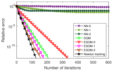
Figure 1: Relative errors of Newton tracking, DQM, NN-$K$, and ESOM-$K$ versus number of iterations.

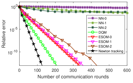
Figure 2: Relative errors of Newton tracking, NN-$K$, ESOM-$K$ and DQM versus rounds of communications.

Fig. 1 illustrates the relative error versus the number of iterations. Observe that NN-$K$ converges to the neighborhoods of optimal argument. Among the exact decentralized algorithms, the proposed Newton tracking algorithm has the best performance compared with the other algorithms and converges linearly, which validates the theoretical result in Theorem 1.

Newton tracking and DQM require one round of communication per iteration. For other algorithms, NN-$K$ and ESOM-$K$ require $K+1$ rounds. Fig. 2 illustrates the relative error versus the rounds of communication. Observe that although ESOM-1 and ESOM-2 perform well as depicted in Fig. 1, they become worse in Fig. 2 because more rounds of communication are required in each iteration. In terms of the communication cost, the proposed Newton tracking algorithm is still the best.

V-B Comparison with First-order Methods

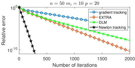
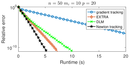
Figure 3: Relative errors of Newton tracking, gradient tracking, EXTRA and DLM when $n=50$, $m_{i}=10$ and $p=20$.

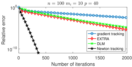
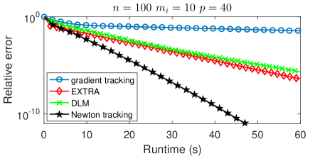
Figure 4: Relative errors of Newton tracking, gradient tracking, EXTRA and DLM when $n=100$, $m_{i}=10$ and $p=40$.

We compare Newton tracking with the first-order algorithms, including gradient tracking [21], EXTRA [15] and DLM [17]. We respectively rewrite these three algorithms as their equivalent updates: (gradient tracking) $\mathbf{x}^{t+2}=2\mathbf{W}\mathbf{x}^{t+1}-\mathbf{W}^{2}\mathbf{x}^{t}-\alpha\left[\nabla f\left(\mathbf{x}^{t+1}\right)-\nabla f\left(\mathbf{x}^{t}\right)\right]$, (EXTRA) $\mathbf{x}^{t+2}=(\mathbf{I}+\mathbf{W})\mathbf{x}^{t+1}-(\mathbf{I}+\mathbf{W})\mathbf{x}^{t}/2-\alpha\left[\nabla f\left(\mathbf{x}^{t+1}\right)-\nabla f\left(\mathbf{x}^{t}\right)\right]$ and (DLM) $\mathbf{x}^{t+2}=\left(\mathbf{I}-\alpha DL_{o}\right)(2\mathbf{x}^{t+1}-\mathbf{x}^{t})-D\left[\nabla f\left(\mathbf{x}^{t+1}\right)-\nabla f\left(\mathbf{x}^{t}\right)\right]$, where $D=\text{diag}\{1/(2\alpha d_{i}+\epsilon)\}$, and $d_{i}$ is the degree of node $i$. $L_{o}$ is the oriented Laplacian defined in [17].

In this section we conduct the experiments under two larger networks. In the second (third) experiments we set the number of nodes as $n=50\;(100)$, the number of samples on each agent as $m_{i}=10\;(10)$ for all $i$ and the dimension of sample vectors as $p=20\;(40)$. The other settings are the same as subsection V-A.

We run all the algorithms with fixed hand-optimized step sizes. The step sizes of gradient tracking and EXTRA in the second (third) experiments are $\alpha=0.16\;(0.6)$ and $\alpha=0.07\;(1.6)$, respectively. The parameters of DLM in the second (third) experiments are $\alpha=0.1\;(0.008)$ and $\epsilon=0.1\;(0.001)$. For Newton tracking, the parameters in the second (third) experiments are $\alpha=1.1\;(0.08)$ and $\epsilon=1.2\;(0.08)$.

Fig. 3 illustrates the relative error versus the number of iterations and runtime, respectively. Observe that the proposed Newton tracking outperforms the first-order algorithms in terms of either the number of iterations or runtime. Although Newton tracking computes the inverse of estimated Hessian $\nabla^{2}f_{i}(x_{i})+\epsilon I_{p}\in\mathbb{R}^{p\times p}$ in each iteration, it calls for relatively smaller number of iterations compared with the first-order algorithms, which leads to the shorter runtime. We get similar results in the third experiments, see Fig. 4.

V-C Effect of Network Topology

This section investigates the performance of Netwon tracking in four different topologies including line graph, cycle graph, random graphs with $\tau=\{0.3,0.5,0.7\}$, and complete graph. The parameters of Newton tracking are set as $\alpha=2.3$ and $\epsilon=2.4$. All the other settings are the same as those in subsection V-A.

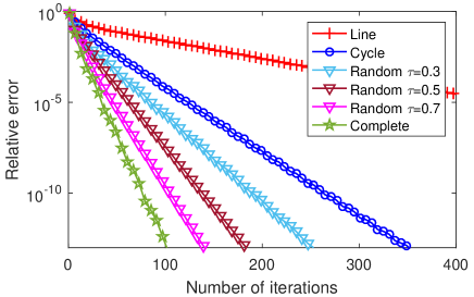
Figure 5: Relative errors of Newton tracking versus number of iterations for line graph, cycle graph, random graphs with $\tau=\{0.3,0.5,0.7\}$, and complete graph.

Fig. 5 illustrates the relative errors versus the number of iterations. Observe that the proposed Newton tracking algorithm has linear convergence rates in all types of graphs. Among them, complete graph yields the fastest speed. This observation confirms the convergence rate developed in Theorem 1. To be specific, for line graph, cycle graph, random graphs with $\tau=\{0.3,0.5,0.7\}$, and complete graph, we have $\hat{\lambda}_{\min}(\mathbf{I}-\mathbf{W})=\{0.03,0.12,0.17,0.34,0.43,1.00\}$ and ${\lambda}_{\max}(\mathbf{I}-\mathbf{W})=\{1.30,1.33,1.16,1.15,1.10,1.00\}$, respectively. According to the definition of $\delta^{\prime}$ in (61), the complete graph with the largest $\hat{\lambda}_{\min}(\mathbf{I}-\mathbf{W})$ and the smallest ${\lambda}_{\max}(\mathbf{I}-\mathbf{W})$ has the largest $\delta^{\prime}$, and hence the fastest convergence speed.

VI CONCLUSIONS

This paper proposed a novel Newton tracking algorithm to solve the decentralized consensus optimization problem. Each node updates its local variable along a modified local Newton direction, which is calculated with neighboring and historical information. Newton tracking employs a fixed step size and, yet, converges to an exact solution. The connections between Newton tracking and several existing methods, including gradient tracking and second-order algorithms were investigated. We proved that the proposed algorithm converges at a linear rate under the strongly convex assumption. Numerical experiments demonstrated the efficacy of Newton tracking, compared with existing algorithms such as gradient tracking, NN, ESOM, and DQM.

References

• [1] S. Pu, W. Shi, J. Xu, and A. Nedić, “A push-pull gradient method for distributed optimization in networks,” in IEEE Conference on Decision and Control, 2018, pp. 3385–3390.
• [2] Y. Liu, F. R. Yu, X. Li, H. Ji, and V. C. Leung, “Decentralized resource allocation for video transcoding and delivery in blockchain-based system with mobile edge computing,” IEEE Transactions on Vehicular Technology, vol. 68, no. 11, pp. 11 169–11 185, 2019.
• [3] D.-T. Ta, K. Khawam, S. Lahoud, C. Adjih, and S. Martin, “LoRa-MAB: A flexible simulator for decentralized learning resource allocation in IoT networks,” in IFIP Wireless and Mobile Networking Conference, 2019, pp. 55–62.
• [4] E. Dall’Anese, H. Zhu, and G. B. Giannakis, “Distributed optimal power flow for smart microgrids,” IEEE Transactions on Smart Grid, vol. 4, no. 3, pp. 1464–1475, 2013.
• [5] H. J. Liu, W. Shi, and H. Zhu, “Hybrid voltage control in distribution networks under limited communication rates,” IEEE Transactions on Smart Grid, vol. 10, no. 3, pp. 2416–2427, 2019.
• [6] A. Lalitha, S. Shekhar, T. Javidi, and F. Koushanfar, “Fully decentralized federated learning,” in Advances in Neural Information Processing Systems Workshop on Bayesian Deep Learning, 2018.
• [7] T. Li, A. K. Sahu, A. Talwalkar, and V. Smith, “Federated learning: Challenges, methods, and future directions,” arXiv preprint arXiv:1908.07873, 2019.
• [8] Y. Zhao, J. Zhao, L. Jiang, R. Tan, and D. Niyato, “Mobile edge computing, blockchain and reputation-based crowdsourcing IoT federated learning: A secure, decentralized and privacy-preserving system,” arXiv preprint arXiv:1906.10893, 2019.
• [9] X. Lian, C. Zhang, H. Zhang, C.-J. Hsieh, and J. Liu, “Can decentralized algorithms outperform centralized algorithms? A case study for decentralized parallel stochastic gradient descent,” in Advances in Neural Information Processing Systems, 2017.
• [10] A. Koppel, S. Paternain, C. Richard, and A. Ribeiro, “Decentralized online learning with kernels,” IEEE Transactions on Signal Processing, vol. 66, no. 12, pp. 3240–3255, 2018.
• [11] D. Lee, N. He, P. Kamalaruban, and V. Cevher, “Optimization for reinforcement learning: From single agent to cooperative agents,” arXiv preprint arXiv:1912.00498, 2019.
• [12] A. Nedic and A. Ozdaglar, “Distributed subgradient methods for multi-agent optimization,” IEEE Transactions on Automatic Control, vol. 54, no. 1, pp. 48–61, 2009.
• [13] K. Yuan, Q. Ling, and W. Yin, “On the convergence of decentralized gradient descent,” SIAM Journal on Optimization, vol. 26, no. 3, pp. 1835–1854, 2016.
• [14] D. Jakovetić, J. Xavier, and J. M. Moura, “Fast distributed gradient methods,” IEEE Transactions on Automatic Control, vol. 59, no. 5, pp. 1131–1146, 2014.
• [15] W. Shi, Q. Ling, G. Wu, and W. Yin, “EXTRA: An exact first-order algorithm for decentralized consensus optimization,” SIAM Journal on Optimization, vol. 25, no. 2, pp. 944–966, 2015.
• [16] W. Shi, Q. Ling, K. Yuan, G. Wu, and W. Yin, “On the linear convergence of the ADMM in decentralized consensus optimization,” IEEE Transactions on Signal Processing, vol. 62, no. 7, pp. 1750–1761, 2014.
• [17] Q. Ling, W. Shi, G. Wu, and A. Ribeiro, “DLM: Decentralized linearized alternating direction method of multipliers,” IEEE Transactions on Signal Processing, vol. 63, no. 15, pp. 4051–4064, 2015.
• [18] K. Yuan, B. Ying, X. Zhao, and A. H. Sayed, “Exact diffusion for distributed optimization and learning – Part I: Algorithm development,” IEEE Transactions on Signal Processing, vol. 67, no. 3, pp. 708–723, 2018.
• [19] Z. Li, W. Shi, and M. Yan, “A decentralized proximal-gradient method with network independent step-sizes and separated convergence rates,” IEEE Transactions on Signal Processing, vol. 67, no. 17, pp. 4494–4506, 2019.
• [20] J. Xu, S. Zhu, Y. C. Soh, and L. Xie, “Augmented distributed gradient methods for multi-agent optimization under uncoordinated constant stepsizes,” in IEEE Conference on Decision and Control, 2015, pp. 2055–2060.
• [21] G. Qu and N. Li, “Harnessing smoothness to accelerate distributed optimization,” IEEE Transactions on Control of Network Systems, vol. 5, no. 3, pp. 1245–1260, 2017.
• [22] R. Xin and U. A. Khan, “A linear algorithm for optimization over directed graphs with geometric convergence,” IEEE Control Systems Letters, vol. 2, no. 3, pp. 315–320, 2018.
• [23] Y. Sun, A. Daneshmand, and G. Scutari, “Convergence rate of distributed optimization algorithms based on gradient tracking,” arXiv preprint arXiv:1905.02637, 2019.
• [24] R. Xin, S. Kar, and U. A. Khan, “Gradient tracking and variance reduction for decentralized optimization and machine learning,” arXiv preprint arXiv:2002.05373, 2020.
• [25] A. Mokhtari, Q. Ling, and A. Ribeiro, “Network Newton distributed optimization methods,” IEEE Transactions on Signal Processing, vol. 65, no. 1, pp. 146–161, 2016.
• [26] D. Bajovic, D. Jakovetic, N. Krejic, and N. K. Jerinkic, “Newton-like method with diagonal correction for distributed optimization,” SIAM Journal on Optimization, vol. 27, no. 2, pp. 1171–1203, 2017.
• [27] F. Mansoori and E. Wei, “A fast distributed asynchronous Newton-based optimization algorithm,” arXiv preprint arXiv:1901.01872, 2019.
• [28] A. Mokhtari, W. Shi, Q. Ling, and A. Ribeiro, “DQM: Decentralized quadratically approximated alternating direction method of multipliers,” IEEE Transactions on Signal Processing, vol. 64, no. 19, pp. 5158–5173, 2016.
• [29] ——, “A decentralized second-order method with exact linear convergence rate for consensus optimization,” IEEE Transactions on Signal and Information Processing over Networks, vol. 2, no. 4, pp. 507–522, 2016.
• [30] M. Eisen, A. Mokhtari, and A. Ribeiro, “A primal-dual quasi-Newton method for exact consensus optimization,” IEEE Transactions on Signal Processing, vol. 67, no. 23, pp. 5983–5997, 2019.
• [31] S. Soori, K. Mischenko, A. Mokhtari, M. M. Dehnavi, and M. Gurbuzbalaban, “DAve-QN: A distributed averaged quasi-Newton method with local superlinear convergence rate,” arXiv preprint arXiv:1906.00506, 2019.
• [32] J. Zhang, K. You, and T. Başar, “Distributed adaptive Newton methods with globally superlinear convergence,” arXiv preprint arXiv:2002.07378, 2020.
• [33] S. Boyd, P. Diaconis, and L. Xiao, “Fastest mixing Markov chain on a graph,” SIAM Review, vol. 46, no. 4, pp. 667–689, 2004.
• [34] S. U. Pillai, T. Suel, and S. Cha, “The Perron-Frobenius theorem: Some of its applications,” IEEE Signal Processing Magazine, vol. 22, no. 2, pp. 62–75, 2005.