Learning Dynamical Systems with Side Information$\dagger$

Abstract

We present a mathematical and computational framework for the problem of learning a dynamical system from noisy observations of a few trajectories and subject to side information. Side information is any knowledge we might have about the dynamical system we would like to learn besides trajectory data. It is typically inferred from domain-specific knowledge or basic principles of a scientific discipline. We are interested in explicitly integrating side information into the learning process in order to compensate for scarcity of trajectory observations. We identify six types of side information that arise naturally in many applications and lead to convex constraints in the learning problem. First, we show that when our model for the unknown dynamical system is parameterized as a polynomial, one can impose our side information constraints computationally via semidefinite programming. We then demonstrate the added value of side information for learning the dynamics of basic models in physics and cell biology, as well as for learning and controlling the dynamics of a model in epidemiology. Finally, we study how well polynomial dynamical systems can approximate continuously-differentiable ones while satisfying side information (either exactly or approximately). Our overall learning methodology combines ideas from convex optimization, real algebra, dynamical systems, and functional approximation theory, and can potentially lead to new synergies between these areas.

1 Motivation and problem formulation

In several safety-critical applications, one has to learn the behavior of an unknown dynamical system from noisy observations of a very limited number of trajectories. For example, to autonomously land an airplane that has just gone through engine failure, limited time is available to learn the modified dynamics of the plane before appropriate control action can be taken. Similarly, when a new infectious disease breaks out, few observations are initially available to understand the dynamics of contagion. In situations of this type where data is limited, it is essential to exploit “side information”—e.g. physical laws or contextual knowledge—to assist the task of learning.

More formally, our interest in this paper is to learn a continuous-time dynamical system of the form

(1) $$\dot{x}(t)=f(x(t)),$$

over a given compact set $\Omega\subset\mathbb{R}^{n}$ from noisy observations of a limited number of its trajectories. Here, $\dot{x}(t)$ denotes the time derivative of the state $x(t)\in\mathbb{R}^{n}$ at time $t$. We assume that the unknown vector field $f$ that is to be learned is continuously differentiable over an open set containing $\Omega$, an assumption that is often met in applications. In our setting, we have access to a training set of the form

(2) $$\mathcal{D}\coloneqq\{(x_{i},{y}_{i}),\quad i=1,\ldots,N\},$$

where $x_{i}\in\Omega$ (resp. ${y}_{i}\in\mathbb{R}^{n}$) is a possibly noisy measurement of the state of the dynamical system (resp. of $f(x_{i})$). Typically, this training set is obtained from observation of a few trajectories of (1). The vectors $y_{i}$ could be either directly accessible (e.g., from sensor measurements) or approximated from the state variables using a finite-difference scheme.

Finding a vector field $f_{\mathcal{F}}$ that best agrees with the training set $\mathcal{D}$ among a particular class $\mathcal{F}$ of continuously-differentiable functions amounts to solving the optimization problem

(3) $$f_{\mathcal{F}}\in\underset{p\in\mathcal{F}}{\arg\min}\sum_{(x_{i},{y}_{i})\in\mathcal{D}}\ell(p(x_{i}),{y}_{i}),$$

where $\ell(\cdot,\cdot)$ is some loss function that penalizes deviation of $p(x_{i})$ from $y_{i}$. For instance, $\ell(\cdot,\cdot)$ could simply be the $\ell_{2}$ loss function

$$\ell_{2}(u,v)\coloneqq\|u-v\|_{2}\quad\forall u,v\in\mathbb{R}^{n},$$

though the computational machinery that we propose can readily handle various other convex loss functions (see Section 3).

In addition to fitting the training set $\mathcal{D}$, we desire for our learned vector field $f_{\mathcal{F}}$ to generalize well, i.e., to be consistent as much as possible with the behavior of the unknown vector field $f$ on all of $\Omega$. Indeed, the optimization problem in (3) only dictates how the candidate vector field should behave on the training data. This could easily lead to overfitting, especially if the function class $\mathcal{F}$ is large and the observations are limited. Let us demonstrate this phenomenon by a simple example.

Example 1.

Consider the two-dimensional vector field

(4) $$f(x_{1},x_{2})\coloneqq(-x_{2},x_{1})^{T}.$$

The trajectories of the system $\dot{x}(t)=f(x(t))$ from any initial condition are given by circular orbits. In particular, if started from the initial condition $x_{\text{init}}=(1,0)^{T}$, the trajectory is given by $x(t,x_{\text{init}})=(\cos(t),\sin(t))^{T}$. Hence, for any function $g:\mathbb{R}^{2}\rightarrow\mathbb{R}^{2},$ the vector field

(5) $$h(x)\coloneqq f(x)+(x_{1}^{2}+x_{2}^{2}-1)g(x)$$

agrees with $f$ on the sample trajectory $x(t,x_{\text{init}})$. However, the behavior of the trajectories of $h$ depends on the arbitrary choice of the function $g$. If $g(x)=x$ for instance, the trajectories of $h$ starting outside of the unit disk diverge to infinity. See Fig. 1 for an illustration.

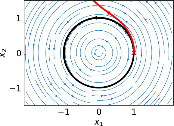
Figure 1: Streamplot of the vector field $f$ in (4) (in blue), together with two sample trajectories of the vector field $h$ in (5) with $g(x)=x$ when started from $(1,0)^{T}$ (drawn in black) and from $(1.01,0)^{T}$ (drawn in red). The trajectories of $f$ and $h$ match exactly when started from $(1,0)^{T}$, but get arbitrarily far from each other when started from $(1.01,0)^{T}$.

To address the issue of insufficiency of data and to avoid overfitting, we would like to exploit the fact that in many applications, one may have contextual information about the vector field $f$ without knowing $f$ precisely. We call such contextual information side information. Formally, every side information is a subset $S$ of the set of all continuously-differentiable functions that the vector field $f$ is known to belong to. Equipped with a list of side information $S_{1},\ldots,S_{k}$, our goal is to replace the optimization problem in (3) with

(6) $$f_{\mathcal{F}\cap S_{1}\cap\dots\cap S_{k}}\in\underset{p\in\mathcal{F}\cap S_{1}\cap\dots\cap S_{k}}{\arg\min}\sum_{(x_{i},{y}_{i})\in\mathcal{D}}\ell(p(x_{i}),{y}_{i}),$$

i.e., to find a vector field $f_{\mathcal{F}\cap S_{1}\cap\dots\cap S_{k}}\in\mathcal{F}$ that is closest to $f$ on the training set $\mathcal{D}$ and also satisfies the side information $S_{1},\ldots,S_{k}$ that $f$ is known to satisfy.

1.1 Outline and contributions of the paper

In the remainder of this paper, we build on the mathematical formalism we have introduced thus far and make problem (6) more concrete and amenable to computation. In Section 2, we identify six notions of side information that are commonly encountered in practice and that have attractive convexity properties, therefore leading to a convex optimization formulation of problem (6). In Section 3, we show that when the function class $\mathcal{F}$ is chosen as the set of polynomial functions of a given degree, then any combination of our six notions of side information can be enforced by semidefinite programming. The derivation of these semidefinite programs leverages ideas from sum of squares optimization, a concept that we briefly review in the same section for the convenience of the reader. In Section 4, we demonstrate the applicability of our approach on three examples from epidemiology, classical mechanics, and cell biology. In each example, we show how common sense and contextual knowledge translate to the notions of side information we present in this paper. Furthermore, in each case, we show that by imposing side information via semidefinite programming, we can learn the behavior of the unknown dynamics from a very limited set of observations. In our epidemiology example, we also show the benefits of our approach for a downstream task of optimal control (Section 4.5). In Section 5, we study the question of how well trajectories of a continuously differentiable vector field that satisfies some side information can be approximated by trajectories of a polynomial vector field that satisfies the same side information either exactly or approximately. We end the paper with a discussion of future research directions in Section 6.

We emphasize that our aim in this paper is not to propose our framework as an alternative to other learning algorithms, but rather to present a road map for incorporating side information in the problem of learning dynamical systems from data in general. We make this road map more explicit by focusing on the common problem of fitting a polynomial vector field to data. However, our hope is that this work stimulates future research on incorporating side information in many other approaches to learning dynamical systems.

1.2 Related work

The idea of using sum of squares and semidefinite optimization for verifying various properties of a known dynamical system has been the focus of much research in the control and optimization communities [38, 9, 31, 11]. Our work borrows some of these techniques to instead impose a desired set of properties on a candidate dynamical system that is to be learned from data.

Learning dynamical systems from data is an important problem in the field of system identification; see e.g. [12, 26, 5] and references therein. Various classes of vector fields have been proposed throughout the years as candidates for the function class $\mathcal{F}$ in (3); e.g., reproducing kernel Hilbert spaces [45, 47, 14], Guassian mixture models [28], and neural networks [55, 19]. Some recent approaches to learning dynamical systems from data impose additional properties on the candidate vector field. These properties include contraction  [45, 18], stabilizability  [46], and stability [29], and can be thought of as side information. In contrast to our work, imposing these properties requires formulation of nonconvex optimization problems, which can be hard to solve to global optimality. Furthermore, these references impose the desired properties only on sample trajectories (as opposed to the entire space where the properties are known to hold), or introduce an additional layer of nonconvexity to impose the constraints globally.

We also note that the problem of fitting a polynomial vector field to data has appeared e.g. in [44], though the focus there is on imposing sparsity of the coefficients of the vector field as opposed to side information. More generally, the problem of finding sparse representations of dynamical systems form data has been studied in [13], where an algorithm for sparse identification of nonlinear dynamics is introduced. The closest work in the literature to our work is that of Hall on shape-constrained regression [22, Chapter 8], where similar algebraic techniques are used to impose constraints such as convexity and monotonicity on a polynomial regressor. See also [16] for some statistical properties of these regressors and several applications. Our work can be seen as an extension of this approach to a dynamical system setting.

2 Side information

In this section, we identify six types of side information which we believe are useful in practice (see, e.g., Section 4) and that lead to a convex formulation of problem (6). For example, we will see in Section 3 that semidefinite programming can be used to impose any list of side information constraints of the six types below on a candidate vector field that is parameterized as a polynomial function. The set $\Omega$ that appears in these definitions is a compact subset of $\mathbb{R}^{n}$ over which we would like to learn an unknown vector field $f$. Throughout this paper, the notation $f\in{C_{1}^{\circ}(\Omega)}$ denotes that $f$ is continuously differentiable over an open set containing $\Omega$.

• Interpolation at a finite set of points. For a set of points $\{(x_{i},{y}_{i})\in\Omega\times\mathbb{R}^{n}\}_{i=1}^{m},$ we denote by $\operatorname{{\bf Interp}}(\{(x_{i},y_{i})\}_{i=1}^{m})$ the set of vector fields $f\in{C_{1}^{\circ}(\Omega)}$ that satisfy $f(x_{i})~{}=~{}y_{i}$ for $i=1,\dots,m$. An important special case is the setting where the vectors $y_{i}$ are equal to $0$. In this case, the side information is the knowledge of certain equilibrium points of the vector field $f$.

• Group symmetry. For two given linear representations $\sigma,\rho:G\rightarrow\mathbb{R}^{n\times n}$ of a finite group $G$, with $\sigma(g)x\in\Omega\;\forall(x,g)\in\Omega\times G$, we define $\operatorname{{\bf Sym}}(G,\sigma,\rho)$ to be the set of vector fields $f\in{C_{1}^{\circ}(\Omega)}$ that satisfy the symmetry condition

  $$f(\sigma(g)x)=\rho(g)f(x)\;\forall x\in\Omega,\;\forall g\in G.$$

  For example, let $\Omega$ be the unit ball in $\mathbb{R}^{n}$ and consider the group $F_{2}=\{1,-1\}$, with scalar multiplication as the group operation. If we take $\sigma_{F_{2}}$ to be the linear representation of $F_{2}$ defined by $\sigma_{F_{2}}(1)=-\sigma_{F_{2}}(-1)=I$, where $I$ denotes the $n\times n$ identity matrix, then a vector field $f\in{C_{1}^{\circ}(\Omega)}$ is in $\operatorname{{\bf Sym}}(F_{2},\sigma_{F_{2}},\sigma_{F_{2}})$ if and only if

  $$f(\sigma_{F_{2}}(1)x)=\sigma_{F_{2}}(1)f(x)\text{ and }f(\sigma_{F_{2}}(-1)x)=\sigma_{F_{2}}(-1)f(x)\;\forall x\in\Omega,$$

  that is

  $$f(x)=-f(x)\;\forall x\in\Omega.$$

  In other words, the set $\operatorname{{\bf Sym}}(F_{2},\sigma_{F_{2}},\sigma_{F_{2}})$ is exactly the set of even vector fields in ${C_{1}^{\circ}(\Omega)}$. Similarly, if we take $\rho_{F_{2}}$ to be the linear representation of $F_{2}$ defined by $\rho_{F_{2}}(1)=\rho_{F_{2}}(-1)=I$, then $\operatorname{{\bf Sym}}(F_{2},\sigma_{F_{2}},\rho_{F_{2}})$ is the set of odd vector fields in ${C_{1}^{\circ}(\Omega)}$. As another example, consider the group $S_{n}$ of all permutations of the set $\{1,\ldots,n\}$, with composition as the group operation. If we take $\sigma_{S_{n}}$ to be the map that assigns to an element $p\in S_{n}$ the permutation matrix $P$ obtained by shuffling the columns of the identity matrix according to $p$, and $\rho_{S_{n}}$ to be the constant map that assigns the identity matrix to every $p~{}\in~{}S_{n}$, then the set $\operatorname{{\bf Sym}}(S_{n},\sigma_{S_{n}},\rho_{S_{n}})$ is the set of symmetric functions in ${C_{1}^{\circ}(\Omega)}$, i.e., functions in ${C_{1}^{\circ}(\Omega)}$ that are invariant under permutations of their arguments. We remark that a finite combination of side information of type $\operatorname{{\bf Sym}}$ can often be written equivalently as a single side information of type $\operatorname{{\bf Sym}}$. For example, the set $\operatorname{{\bf Sym}}(F_{2},\sigma_{F_{2}},\rho_{F_{2}})\cap\operatorname{{\bf Sym}}(S_{n},\sigma_{S_{n}},\rho_{S_{n}})$ of even symmetric functions in ${C_{1}^{\circ}(\Omega)}$ is equal to $\operatorname{{\bf Sym}}(F_{2}\times S_{n},\sigma,\rho)$, where $F_{2}\times S_{n}$ is the direct product of $F_{2}$ and $S_{n}$, $\sigma$ is given by $\sigma(g,g^{\prime})=\sigma_{F_{2}}(g)\sigma_{S_{n}}(g^{\prime})\,\forall(g,g^{\prime})\in F_{2}\times S_{n}$, and $\rho$ is the constant map that assigns the identity matrix to every element in $F_{2}\times S_{n}$.

• Coordinate nonnegativity. For given sets $P_{i},N_{i}\subseteq{\Omega}$, $i=1,\ldots,n$, we denote by $\operatorname{{\bf Pos}}(\{(P_{i},N_{i})\}_{i=1}^{n})$ the set of vector fields $f\in{C_{1}^{\circ}(\Omega)}$ that satisfy

  $$f_{i}(x)\geq 0\;\forall x\in P_{i},\text{ and }f_{i}(x)\leq 0\;\forall x\in N_{i},\;\forall i\in\{1,\dots,n\}.$$

  These constraints are useful when we know that certain components of the state vector are increasing or decreasing functions of time in some regions of the state space.

• Coordinate directional monotonicity. For given sets $P_{ij},N_{ij}\subseteq\Omega$, $i,j=1,\ldots,n$, we denote by $\operatorname{{\bf Mon}}(\{(P_{ij},N_{ij})\}_{i,j=1}^{n})$ the set of vector fields $f\in{C_{1}^{\circ}(\Omega)}$ that satisfy

  $$\frac{\partial f_{i}}{\partial x_{j}}(x)\geq 0\;\forall x\in P_{ij},\text{ and }\frac{\partial f_{i}}{\partial x_{j}}(x)\leq 0\;\forall x\in N_{ij},\;\forall i,j\in\{1,\dots,n\}.$$

  See Fig. 2 for an illustration of a simple example.

  Figure 2: An example of the behavior of a vector field $f:\mathbb{R}^{2}\rightarrow\mathbb{R}^{2}$ satisfying $\operatorname{{\bf Mon}}(\{(P_{ij},N_{ij})\}_{i,j=1}^{2})$ with $P_{21}=N_{11}=[0,1]\times\{0\}$ (i.e., $\frac{\partial f_{2}}{\partial x_{1}}(x_{1},0)~{}\geq~{}0\text{ and }\frac{\partial f_{1}}{\partial x_{1}}(x_{1},0)\leq 0\;\forall x_{1}\in[0,1]$), and with the rest of the sets $P_{ij}$ and $N_{ij}$ equal to the empty set.

  In the special case where $P_{ij}=\mathbb{R}^{n}$ and $N_{ij}=\emptyset$ for all $i,j\in\{1,\ldots,n\}$ with $i\neq j$, and $P_{ii}=N_{ii}=\emptyset$ for all $i\in\{1,\ldots,n\}$, the side information is the knowledge of the following property of the vector field $f$ which appears frequently in the literature on monotone systems [49]:

  $$\forall x_{\text{init}},\tilde{x}_{\text{init}}\in\mathbb{R}^{n},\quad x_{\text{init}}\leq\tilde{x}_{\text{init}}\implies x(t,x_{\text{init}})\leq x(t,\tilde{x}_{\text{init}})\;\forall t\geq 0.$$

  Here, the inequalities are interpreted elementwise, and the notation $x(t,x_{\text{init}})$ is used as before to denote the trajectory of the vector field $f$ starting from the initial condition $x_{\text{init}}$.

• Invariance of a set. A set $B\subseteq\Omega$ is invariant under a vector field $f$ if any trajectory of the dynamical system $\dot{x}(t)=f(x(t))$ which starts in $B$ stays in $B$ forever. In particular, if $B=\{x\in\mathbb{R}^{n}\;|\;h_{j}(x)\geq 0,\;j=1,,\dots,m\}$ for some differentiable functions $h_{j}:\mathbb{R}^{n}\rightarrow\mathbb{R}$, then invariance of the set $B$ under the vector field $f$ implies the following constraints (see Figure 3 for an illustration):

  (7) $$\forall j\in\{1,\ldots,m\},\;\forall x\in B,\quad\left[h_{j}(x)=0\implies\langle f(x),\nabla h_{j}(x)\rangle\geq 0\right].$$

  Indeed, suppose for some $\tilde{x}\in B$ and for some $j\in\{1,\ldots,m\}$, we had $h_{j}(\tilde{x})=0$ but $\langle f(\tilde{x}),\nabla h_{j}(\tilde{x})\rangle=\dot{h}(\tilde{x})<0$, then $h(x(t,\tilde{x}))<0$ for $t$ small enough, implying that $x(t,\tilde{x})\not\in B$ for $t$ small enough. It is also straightforward to verify that if the “$\geq$” in (7) were replaced with a “$>$”, then the resulting condition would be sufficient for invariance of the set $B$ under $f$. In fact, it follows from a theorem of Nagumo [37, 8] that condition (7) is necessary and sufficient for invariance of the set $B$ under $f$ if $B$ is convex, the functions $h_{1},\ldots,h_{m}$ are continuously-differentiable, and for every point $x$ on the boundary of $B$, the vectors $\{\nabla h_{j}(x)\;|\;j\in\{1,\ldots,m\},h_{j}(x)=0\}$ are linearly independent. Given sets $B_{i}=\{x\in\mathbb{R}^{n}\;|\;h_{ij}(x)\geq 0,\;j=1,,\dots,m_{i}\}$, $i=1,\ldots,r$, defined by differentiable functions $h_{ij}:\mathbb{R}^{n}\rightarrow\mathbb{R}$, we denote by $\operatorname{{\bf Inv}}(\{B_{i}\}_{i=1}^{r})$ the set of all vector fields $f\in{C_{1}^{\circ}(\Omega)}$ that satisfy (7) for $B\in\{B_{1},\ldots,B_{r}\}$.

  Figure 3: An example of the behavior of a vector field $f:\mathbb{R}^{2}\rightarrow\mathbb{R}^{2}$ satisfying $\operatorname{{\bf Inv}}(\{B\})$, where $B\coloneqq\{x\in\mathbb{R}^{2}\;|\;h_{1}(x)\geq 0,\ldots,h_{m}(x)\geq 0\}$ is the set shaded in gray.

• Gradient and Hamiltonian systems. A vector field $f\in{C_{1}^{\circ}(\Omega)}$ is said to be a gradient vector field if there exists a differentiable, scalar-valued function $V:\mathbb{R}^{n}\rightarrow\mathbb{R}$ such that

  (8) $$f(x)=-\nabla V(x)\;\forall x\in\Omega.$$

  Typically, the function $V$ is interpreted as a notion of potential or energy associated with the dynamical system $\dot{x}(t)=f(x(t))$. Note that the value of the function $V$ decreases along the trajectories of this dynamical system. We denote by $\operatorname{{\bf Grad}}$ the subset of ${C_{1}^{\circ}(\Omega)}$ consisting of gradient vector fields.

  A vector field $f\in{C_{1}^{\circ}(\Omega)}$ over $n$ state variables $(x_{1},\ldots,x_{n})$ is said to be Hamiltonian if $n$ is even and there exists a differentiable scalar-valued function $H:\mathbb{R}^{n}\rightarrow\mathbb{R}$ such that

  $$f_{i}(p,q)=-\frac{\partial H}{\partial q_{i}}(p,q),f_{\frac{n}{2}+i}(p,q)=\frac{\partial H}{\partial p_{i}}(p,q),\;{\forall(p,q)\in\Omega},\;\forall i\in\left\{1,\ldots,\frac{n}{2}\right\},$$

  where $p\coloneqq(x_{1},\ldots,x_{\frac{n}{2}})^{T}$ and $q\coloneqq(x_{\frac{n}{2}+1},\ldots,x_{n})^{T}$. The states ${p}$ and ${q}$ are usually referred to as generalized momentum and generalized position respectively, following terminology from physics. Note that a Hamiltonian system conserves the quantity $H$ along its trajectories. We denote by $\operatorname{{\bf Ham}}$ the subset of ${C_{1}^{\circ}(\Omega)}$ consisting of Hamiltonian vector fields. For related work on learning Hamiltonian systems, see [3, 21].

3 Learning Polynomial Vector Fields Subject to Side Information

In this paper, we take the function class $\mathcal{F}$ in (6) to be the set of polynomial vector fields of a given degree $d$, i.e., polynomial vector fields whose monomials have degree at most $d$. We denote this function class by

$${\mathcal{P}_{d}}\coloneqq\{p:\mathbb{R}^{n}\rightarrow\mathbb{R}^{n}\;|\;p_{i}\text{ is a (scalar-valued) polynomial of degree $d$ for $i=1,\ldots,n$}\}.$$

Furthermore, we assume that the set $\Omega$ over which we would like to learn the unknown dynamical system, the sets $P_{i},N_{i}$ in the definition of $\operatorname{{\bf Pos}}(\{(P_{i},N_{i})\}_{i=1}^{n})$, the sets $P_{ij},N_{ij}$ in the definition of $\operatorname{{\bf Mon}}(\{P_{ij},N_{ij}\}_{i,j=1}^{n})$, and the sets $B_{i}$ in the definition of $\operatorname{{\bf Inv}}(\{B_{i}\}_{i=1}^{r})$ are all closed semialgebraic. We recall that a closed basic semialgebraic set is a set of the form

(9) $$\Lambda\coloneqq\{x\in\mathbb{R}^{n}|\ g_{i}(x)\geq 0,i=1,\ldots,m\},$$

where $g_{1},\ldots,g_{m}$ are (scalar-valued) polynomial functions, and that a closed semialgebraic set is a finite union of closed basic semialgebraic sets.

Our choice of working with polynomial functions to describe the vector field and the sets that appear in the side information definitions are motivated by two reasons. The first is that polynomial functions are expressive enough to represent or approximate a large family of functions and sets that appear in applications. The second reason, which shall be made clear shortly, is that because of some connections between real algebra and semidefinite optimization, several side information constraints that are commonly available in practice can be imposed on polynomial vector fields in a numerically tractable fashion.

With our aforementioned choices, the optimization problem in (6) has as decision variables the coefficients of a candidate polynomial vector field $p:\mathbb{R}^{n}\rightarrow\mathbb{R}^{n}$. When the notion of side information is restricted to the six types presented in Section 2, and under the mild assumptions that $\Omega$ is full dimensional (i.e, that it contains an open set), the constraints of (6) are of the following two types:

1. Affine constraints in the coefficients of $p$.

2. Constraints of the type

   (10) $$q(x)\geq 0\ \forall x\in\Lambda,$$

   where $\Lambda$ is a given closed basic semialgebraic set of the form (9), and $q$ is a (scalar-valued) polynomial whose coefficients depend affinely on the coefficients of the vector field $p$.

For example, membership to $\operatorname{{\bf Interp}}(\{(x_{i},y_{i})\}_{i=1}^{m})$, $\operatorname{{\bf Sym}}(G,\sigma,\rho)$, $\operatorname{{\bf Grad}}$, or $\operatorname{{\bf Ham}}$ can be enforced by affine constraints, while membership to $\operatorname{{\bf Pos}}(\{(P_{i},N_{i})\}_{i=1}^{n})$, $\operatorname{{\bf Inv}}(\{B_{i}\}_{i=1}^{r})$, or $\operatorname{{\bf Mon}}(\{(P_{ij},N_{ij})\}_{i,j=1}^{n})$ can be cast as constraints of the type (10). Unfortunately, imposing the latter type of constraints is NP-hard already when $q$ is a quartic polynomial and $\Lambda=\mathbb{R}^{n}$, or when $q$ is quadratic and $\Lambda$ is a polytope (see, e.g., [36]).

An idea pioneered to a large extent by Lasserre [30] and Parrilo [39] has been to write algebraic sufficient conditions for (10) based on the concept of sum of squares polynomials. We say that a polynomial $h$ is a sum of squares (sos) if it can be written as $h=\sum_{i}q_{i}^{2}$ for some polynomials $q_{i}$. Observe that if we succeed in finding sos polynomials $\sigma_{0},\sigma_{1},\ldots,\sigma_{m}$ such that the polynomial identity

(11) $$q(x)=\sigma_{0}(x)+\sigma_{1}(x)g_{1}(x)+\ldots+\sigma_{m}(x)g_{m}(x)$$

holds (for all $x\in\mathbb{R}^{n}$), then, clearly, the constraint in (10) must be satisfied. When the degrees of the sos polynomials $\sigma_{i}$ are bounded above by an integer $r$, we refer to the identity in (11) as the $\text{degree-}r$ sos certificate of the constraint in (10). Conversely, the following celebrated result in algebraic geometry [42] states that if $g_{1},\ldots,g_{m}$ satisfy the so-called “Archimedean property” (a condition slightly stronger than compactness of the set $\Lambda$), then positivity of $q$ on $\Lambda$ guarantees existence of a $\text{degree-}r$ sos certificate for some integer $r$ large enough.

Theorem 3.1 (Putinar’s Positivstellensatz [42]).

Let

$$\Lambda=\{x\in\mathbb{R}^{n}~{}|~{}g_{1}(x)\geq 0,\ldots,g_{m}(x)\geq 0\}$$

and assume that the collection of polynomials $\{g_{1},\ldots,g_{m}\}$ satisfies the Archimedean property, i.e., there exists a positive scalar $R$ such that

$$R^{2}-\sum_{i=1}^{n}x_{i}^{2}=s_{0}(x)+s_{1}(x)g_{1}(x)+\ldots+s_{m}(x)g_{m}(x),$$

where $s_{0},\ldots,s_{m}$ are sos polynomials. For any polynomial $q$, if $q(x)>0\;\forall~{}x~{}\in~{}\Lambda$, then

$$q(x)=\sigma_{0}(x)+\sigma_{1}(x)g_{1}(x)+\ldots+\sigma_{m}(x)g_{m}(x),$$

for some sos polynomials $\sigma_{0},\ldots,\sigma_{m}$.

The computational appeal of the sum of squares approach stems from its connection to semidefinite programming (SDP). We recall that semidefinite programming is the problem of minimizing a linear function of a symmetric matrix over the intersection of the cone of positive semidefinite matrices with an affine subspace. Semidefinite programs can be solved to arbitrary accuracy in time that scales polynomially with their input size; see [53] for a survey of the theory and applications of this subject.

To make the connection between Theorem 3.1 and SDP more clear, we remark that the search for sos polynomials $\sigma_{0},\sigma_{1},\ldots,\sigma_{m}$ of a given degree that verify the polynomial identity in (11) can be automated via SDP. This is true even when some coefficients of the polynomial $q$ are left as decision variables. This claim is a straightforward consequence of the following well-known fact (see, e.g., [38]): A polynomial $h$ of degree $2d$ is a sum of squares if and only if there exists a symmetric matrix $Q$ which is positive semidefinite and verifies the identity

(12) $$h(x)=z(x)^{T}Qz(x),$$

where $z(x)$ denotes the vector of all monomials in $x$ of degree less than or equal to $d$. The size of the matrix $Q$ is ${n+d\choose d}$, which is polynomial in $n$ (resp. $d$) if $d$ (resp. $n$) is fixed. Identity (12) can be written in an equivalent manner as a system of ${n+2d\choose 2d}$ linear equations involving the entries of the matrix $Q$ and the coefficients of the polynomial $h$. These equations come from equating the coefficients of the polynomials appearing on the left and right hand sides of (12). The problem of finding a positive semidefintie matrix $Q$ whose entries satisfy these linear equations is a semidefinite program. For implementation purposes, there exist modeling languages, such as YALMIP [33], SOSTOOLS [40], or SumOfSquares.jl [54], that accept sos constraints on polynomials directly and do the conversion to a semidefinite program in the background. See e.g. [32, 9, 23] for more background on sum of squares techniques.

To end up with a semidefinite programming formulation of problem (6), we also need to take the loss function $\ell$ that appears in the objective function to be semidefinite representable (i.e., we need its epigraph to be the projection of the feasible set of a semidefinite program; see [7, Chapter 3.2] for a discussion on semidefinite representability and several examples). Luckily, many common loss functions in machine learning are semidefinite representable. Examples of such loss functions include (i) any $\ell_{p}$ norm for a rational number $p\geq 1$, or for $p=\infty$, (ii) any convex piece-wise linear function, (iii) any sos-convex polynomial (see e.g. [25] for a definition), and (iv) any positive integer power of the previous three function classes.

4 Illustrative Experiments

In this section, we present numerical experiments from four application domains to illustrate our methodology. The first three applications are learning experiments and the last one involves an optimal control component. In all of our experiments, we use the SDP-based approach explained in Section 3 to tackle problem (6) and take our loss function $\ell(\cdot,\cdot)$ in (6) to be $\ell(u,v)=\|u-v\|_{2}^{2}\quad\forall u,v\in\mathbb{R}^{n}.$ The added value of side information for learning dynamical systems from data will be demonstrated in these experiments.

4.1 Diffusion of a contagious disease

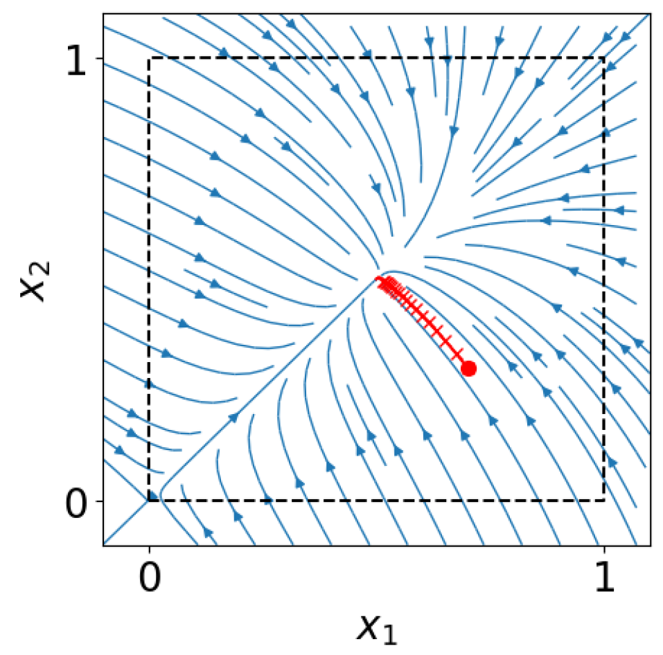
Figure 4: Streamplot of the vector field in (13). We consider this vector field to be the ground truth and unknown to us. We would like to learn it over $[0,1]^{2}$ from noisy snapshots of a single trajectory starting from $(0.7,0.3)^{T}$ (plotted inred).

The following dynamical system has appeared in the epidemiology literature (see, e.g., [4]) as a model for the spread of a sexually transmitted disease in a heterosexual population:

(13) $$\dot{x}(t)=f(x(t)),\text{where}\;x(t)\in\mathbb{R}^{2}\text{ and }f(x)=\left(\begin{array}[]{l}-a_{1}x_{1}+b_{1}(1-x_{1})x_{2}\\ -a_{2}x_{2}+b_{2}(1-x_{2})x_{1}\end{array}\right).$$

Here, the quantity $x_{1}(t)$ (resp. $x_{2}(t)$) represents the fraction of infected males (resp. females) in the population. The parameter $a_{i}$ (resp. $b_{i}$) denotes the recovery rate (resp. the infection rate) in the male population when $i=1$, and in the female population when $i=2$. We take

(14) $$(a_{1},b_{1},a_{2},b_{2})=(0.05,0.1,0.05,0.1)$$

and plot the resulting vector field $f$ in Fig. 4. We suppose that this vector field is unknown to us, and our goal is to learn it over $\Omega\coloneqq[0,1]^{2}$ from a few noisy snapshots of a single trajectory. More specifically, we have access to the training data set

(15) $$\mathcal{D}\coloneqq\left\{\left(x(t_{i},x_{\text{init}}),f(x(t_{i},x_{\text{init}}))+10^{-4}\begin{pmatrix}\varepsilon_{i,1}\\ \varepsilon_{i,2}\end{pmatrix}\right)\right\}_{i=1}^{20},$$

where $x(t,x_{\text{init}})$ is the trajectory of the system (13) starting from the initial condition

$$x_{\text{init}}=(0.7,0.3)^{T},$$

the scalars $t_{i}\coloneqq i$ represent a uniform subdivision of the time interval $[0,20]$, and the scalars $\varepsilon_{1,1},\varepsilon_{1,2},\ldots,\varepsilon_{20,1},\varepsilon_{20,2}$ are independently sampled from the standard normal distribution.

Following our approach in Section 3, we parameterize our candidate vector field

$$p:~{}\mathbb{R}^{2}~{}\rightarrow~{}\mathbb{R}^{2}$$

as a polynomial function. We choose the degree of this polynomial to be $d=3$. The degree $d$ is taken to be larger than $2$ because we do not want to assume knowledge of the degree of the true vector field in (13). This makes the task of learning more difficult; see the end of this subsection where we also learn a vector field of degree $2$ for comparison.

In absence of any side information, one could solve the least-squares problem

(16) $$\min_{p\in\mathcal{P}_{d}}\sum_{(x_{i},{y}_{i})\in\mathcal{D}}\|p(x_{i})-{y}_{i}\|_{2}^{2}$$

to find a polynomial of degree $d$ that best agrees with the training data. For this experiment only, and for educational purposes, we include a template code using the library SumOfSquares.jl [54] of the Julia programming language and demonstrate how the code changes as we impose side information constraints. We initiate our template with the following code that solves optimization problem Eq. 16.

⬇

# Input: vectors $X_{1}$, $X_{2}$, $Y_{1}$, $Y_{2}$ $\in\mathbb{R}^{20}$ representing the training set in (15),

#     where $X_{1}=\{x_{1}(t_{i},x_{\text{init}})\}_{i=1}^{20}$, $X_{2}=\{x_{2}(t_{i},x_{\text{init}})\}_{i=1}^{20}$,

#     $Y_{1}=\{f_{1}(x(t_{i},x_{\text{init}}))+10^{-4}\varepsilon_{i,1}\}_{i=1}^{20}$, and $Y_{2}=\{f_{2}(x(t_{i},x_{\text{init}}))+10^{-4}\varepsilon_{i,2}\}_{i=1}^{20}$

model = SOSModel(solver) # solver could be any SDP solver,

# e.g., Mosek [1], SDPT3 [52], CSDP [10]

@polyvar $x_{1}$ $x_{2}$ # Define state variables $x_{1}$, $x_{2}$

d = 3 # Construct vector of monomials

z = monomials([$x_{1}$, $x_{2}$], 0:d) # in ($x_{1}$, $x_{2}$) up to degree $d$

@variable(model, $p_{1}$, Poly(z)) # Declare a polynomial vector field

@variable(model, $p_{2}$, Poly(z)) # whose coefficients are decision variables

error_vec = [p[1].($X_{1}$, $X_{2}$) - $Y_{1}$; # Vector of individual terms appearing

p[2].($X_{1}$, $X_{2}$) - $Y_{2}$] # in the objective of Eq. 16

@objective model Min error_vec^′ * error_vec

# Side information constraints go here

# …

optimize!(model) # Solve the optimization problem

Julia template code for learning dynamical systems with side information.

The solution to problem (16) returned by the solver MOSEK [1] is plotted in Fig. 5(a). Observe that while the learned vector field replicates the behavior of the true vector field $f$ on the observed trajectory, it differs significantly from $f$ on the rest of the unit square. To remedy this problem, we leverage the following list of side information that is available from the context without knowing the exact structure of $f$.

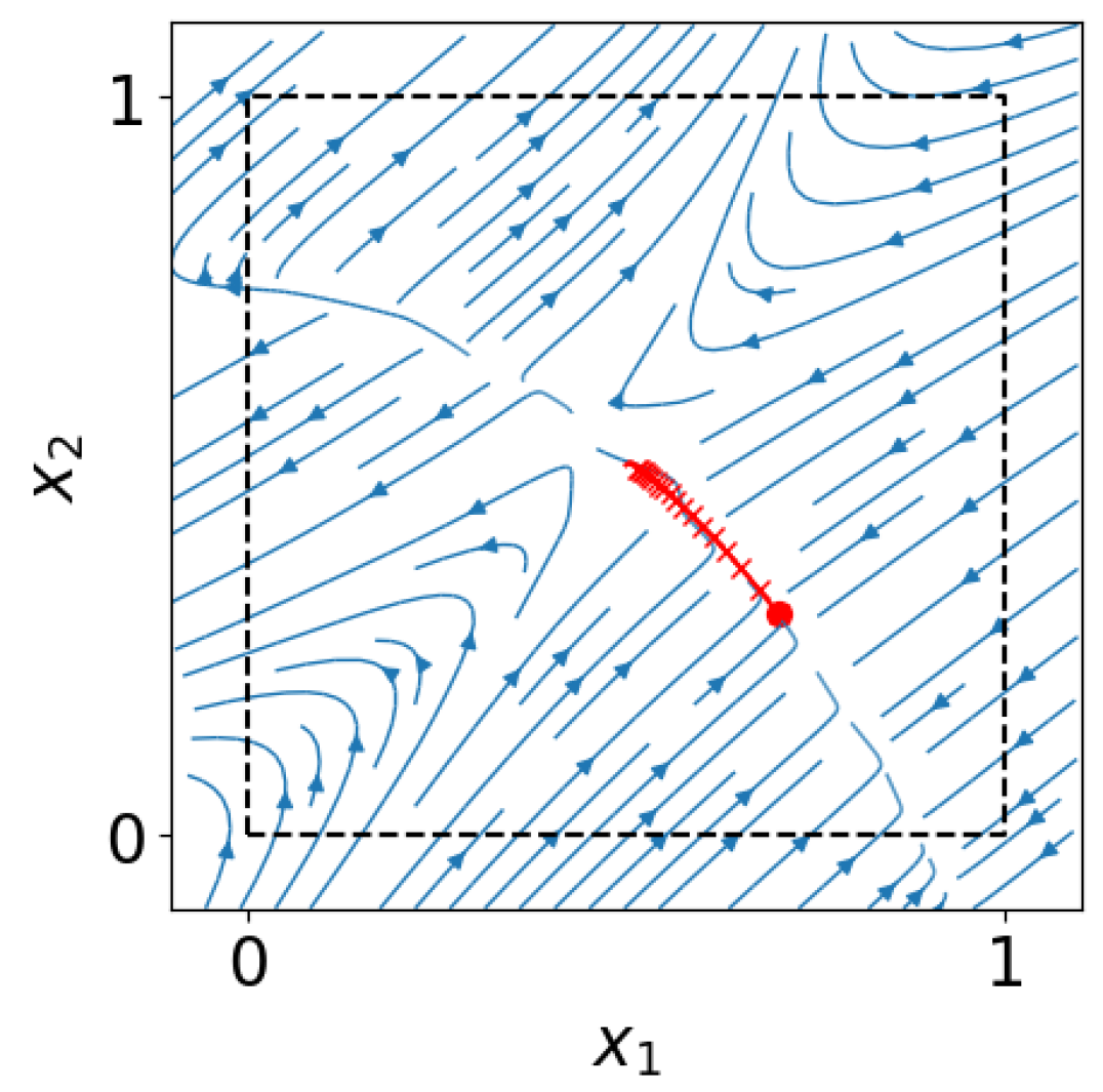
(a) No side information

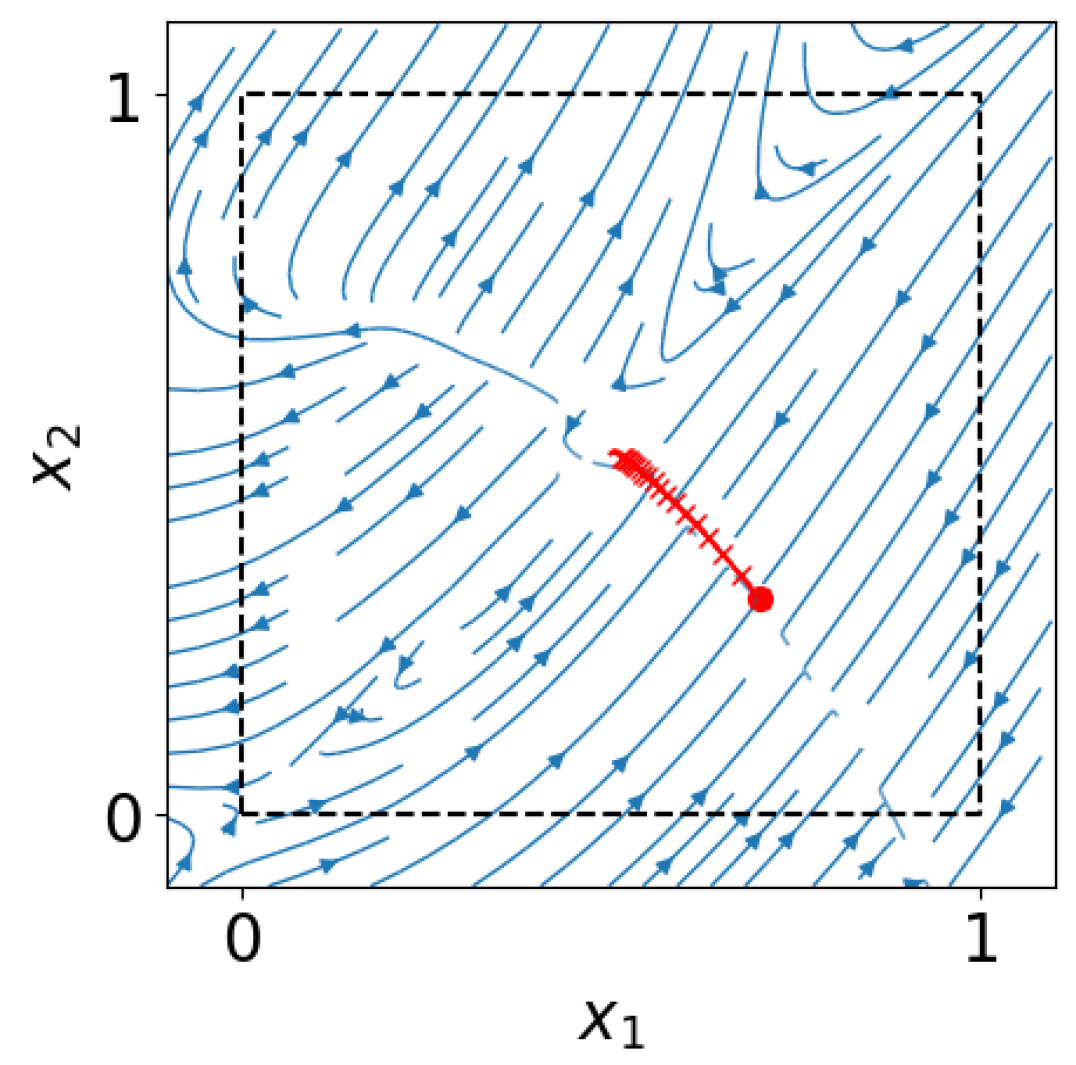
(b) $\operatorname{{\bf Interp}}$

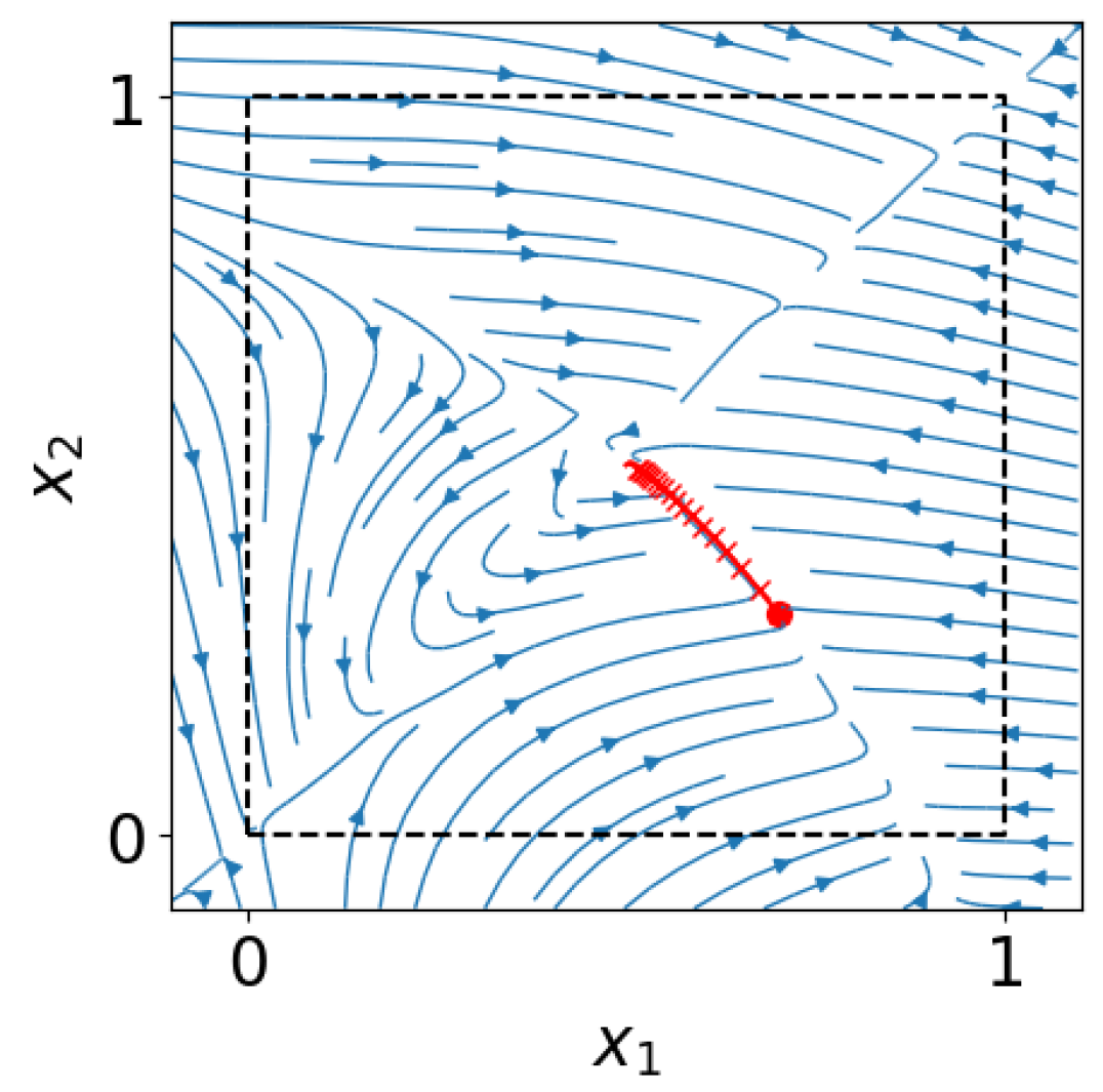
(c) $\operatorname{{\bf Interp}}\cap\operatorname{{\bf Inv}}$

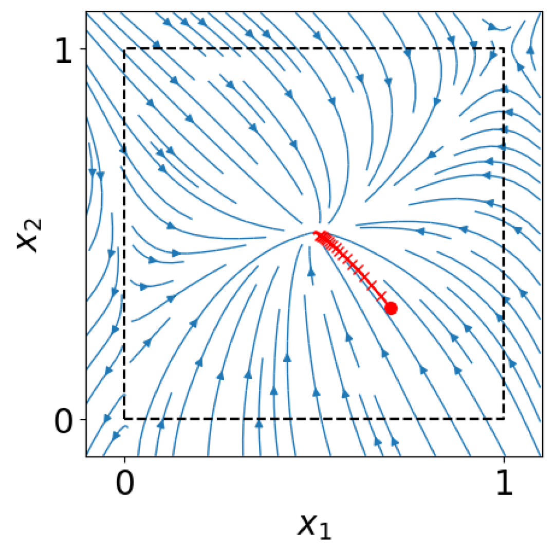
(d) $\operatorname{{\bf Interp}}\cap\operatorname{{\bf Inv}}\cap\operatorname{{\bf Mon}}$

Figure 5: Streamplots of polynomial vector fields of degree $3$ that are optimal to (16) with different side information constraints appended to it.

• Equilibrium point at the origin ($\operatorname{{\bf Interp}}$). Naturally, if no male or female is infected, there would be no contagion and the number of infected individuals will remain at zero. This side information corresponds to our vector field $p$ having an equilibrium point at the origin, i.e., $p(0,0)=0$. Note from Figs. 4 and 5(a) that the true vector field $f$ in (13) satisfies this constraint, but the vector field learned by solving the least-squares problem in (16) does not. We can impose this linear constraint by simply adding the following lines of code to our template:

  ⬇

  @constraint model $p_{1}(0,0)$ == 0

  @constraint model $p_{2}(0,0)$ == 0

  The vector field resulting from solving this new problem is plotted in Fig. 5(b).

• Invariance of the box $[0,1]^{2}$ ($\operatorname{{\bf Inv}}$). The state variables $(x_{1},x_{2})$ of the dynamics in (13) represent fractions of infected individuals and as such, the vector $x(t)$ should be contained in the box $[0,1]^{2}$ at all times $t\geq 0$. Note that this property is violated by the vector fields learned in Figs. 5(a) and 5(b). Mathematically, the invariance of the unit box is equivalent to the four (univariate) polynomial nonnegativity constraints

  $$p_{2}(x_{1},0)\geq 0,p_{2}(x_{1},1)\leq 0\;\forall x_{1}\in[0,1],$$

  $$p_{1}(0,x_{2})\geq 0,p_{1}(1,x_{2})\leq 0\;\forall x_{2}\in[0,1].$$

  These constraints imply that the vector field points inwards on the four edges of the unit box. We replace each one of these four constraints with the corresponding $\text{degree-}2$ sos certificate of the type in (11). For instance, we replace the constraint

  $$p_{2}(x_{1},0)\geq 0\;\forall x_{1}\in[0,1]$$

  with linear and semidefinite constraints obtained from equating the coefficients of the two sides of the polynomial identity

  (17) $$p_{2}(x_{1},0)=x_{1}s_{0}(x_{1})+(1-x_{1})s_{1}(x_{1}),$$

  and requiring that the newly-introduced (univariate) polynomials $s_{0}$ and $s_{1}$ be quadratic and sos. Obviously, the algebraic identity (17) is sufficient for nonnegativity of $p_{2}(x_{1},0)$ over $[0,1]$; in this case, it also happens to be necessary [34]. The code in Julia for imposing the $\text{degree-}2$ sos certificate in (17) is as follows:

  ⬇

  @variable(model, $s_{1}$, Poly([$1,x_{1},x_{1}^{2}$])) # Declare decision polynomial $s_{1}$

  @variable(model, $s_{2}$, Poly([$1,x_{1},x_{1}^{2}$])) # Declare decision polynomial $s_{2}$

  @constraint(model, $s_{1}$, in SOSCone()) # Enforce $s_{1}$ to be sos

  @constraint(model, $s_{2}$, in SOSCone()) # Enforce $s_{2}$ to be sos

  polynomial_identity = # Enfroce polynomial

  $\quad p_{2}((x_{1},x_{2})\Rightarrow(0,x_{2}))$ - $x_{1}$*$s_{1}$-(1-$x_{1}$)*$s_{2}$ # identity in Eq. 17

  @constraint(model,coefficients(polynomial_identity).== 0)

  The output of the semidefinite program which imposes the invariance of the unit box and the equilibrium point at the origin is plotted in Fig. 5(c).

• Coordinate directional monotonicity ($\operatorname{{\bf Mon}}$). Naturally, one would expect that if the fraction of infected males rises in the population, the rate of infection of females should increase. Mathematically, this observation is equivalent to the constraint that

  $$\frac{\partial p_{2}}{\partial x_{1}}(x)\geq 0\;\forall x\in[0,1]^{2}.$$

  Similarly, swapping the roles played by males and females leads to the constraint

  $$\frac{\partial p_{1}}{\partial x_{2}}(x)\geq 0\;\forall x\in[0,1]^{2}.$$

  Note that this property is violated by the vector fields learned in Figs. 5(a), 5(b) and 5(c). Just as in the previous bullet point, we replace each of the above two nonnegativity constraints with its corresponding $\text{degree-}2$ sos certificate. To do this, we represent the closed basic semialgebraic set $[0,1]^{2}$ with the polynomial inequalities

  $$x_{1}\geq 0,x_{2}\geq 0,1-x_{1}\geq 0,1-x_{2}\geq 0.$$

  The Julia code for imposing this side information is similar to the one of the previous bullet point and therefore omitted. Fig. 5(d) demonstrates the vector field learned by our semidefinite program when all side information constraints discussed thus far are imposed.

Note from Figs. 5(a), 5(b), 5(c) and 5(d) that as we add more side information, the learned vector field respects more and more properties of the true vector field $f$. In particular, the learned vector field in Fig. 5(d) is quite similar qualitatively to the true vector field in Fig. 4 even though only noisy snapshots of a single trajectory are used for learning.

It is interesting to observe what would happen if we try to learn a $\text{degree-}2$ vector field from the same training set using the list of side information discussed in this subsection. The outcome of this experiment is plotted in Fig. 6. Note that with the equilibrium-at-the-origin side information, the behavior of the learned vector field of degree $2$ is already quite close to that of the true vector field. Fig. 6(d) shows that when we impose all side information, the learned vector field is almost indistinguishable from the true vector field (even though, once again, only noisy snapshots of a single trajectory are used for learning). The vector field plotted in Fig. 6(d) is given by

$$\small p_{{\operatorname{{\bf Interp}}\cap\operatorname{{\bf Inv}}\cap\operatorname{{\bf Mon}},\text{deg}\;2}}(x_{1},x_{2})=\begin{pmatrix}0.038x_{1}^{2}-0.100x_{1}x_{2}-0.009x_{2}^{2}-0.084x_{1}+0.119x_{2}\\ -0.101x_{1}x_{2}+0.003x_{2}^{2}+0.101x_{1}-0.052x_{2}\end{pmatrix},$$

which is indeed very close to the vector field in (13). For experiments with other degrees and noise levels, see the appendix.

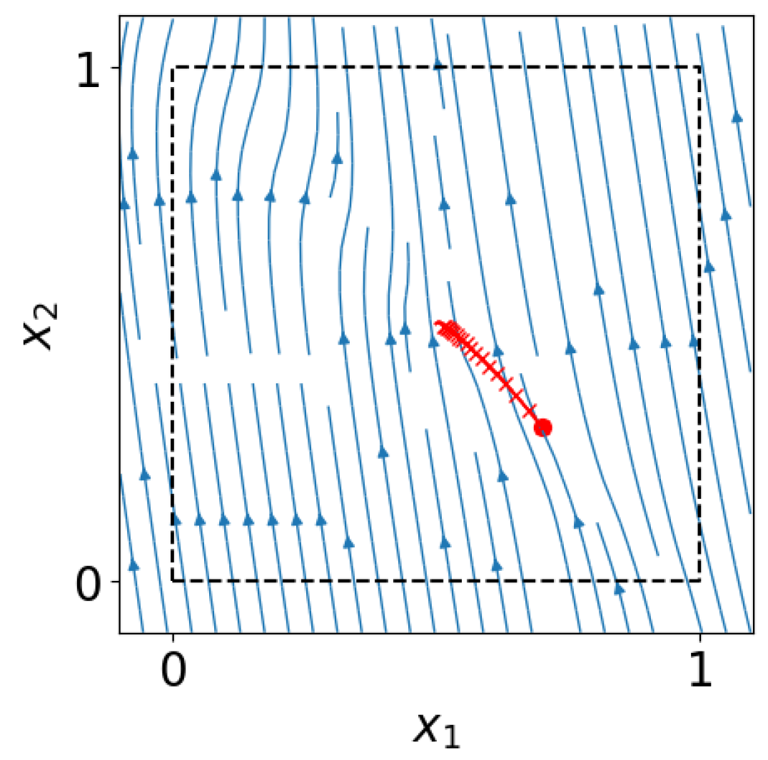
(a) No side information

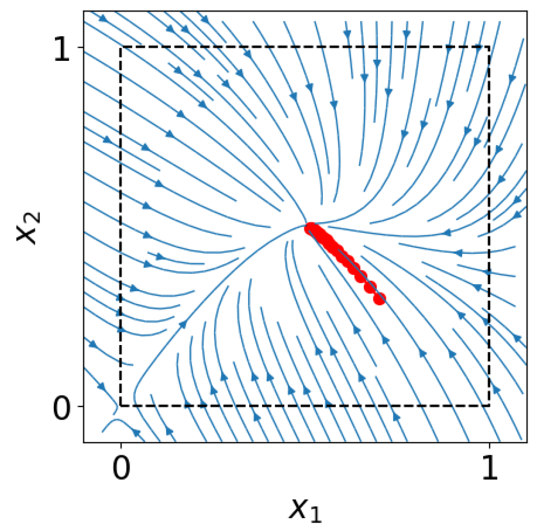
(b) $\operatorname{{\bf Interp}}$

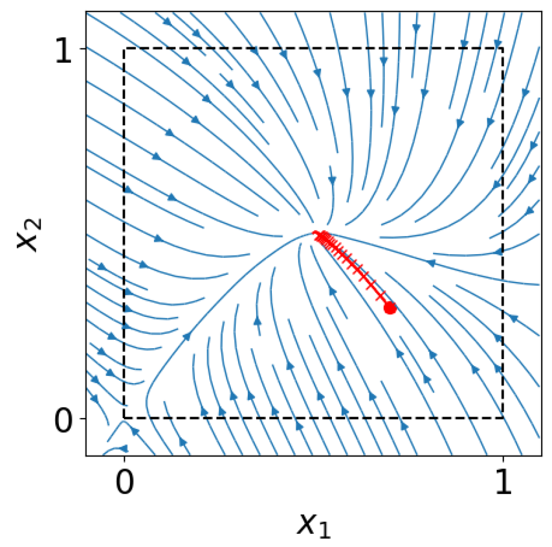
(c) $\operatorname{{\bf Interp}}\cap\operatorname{{\bf Inv}}$

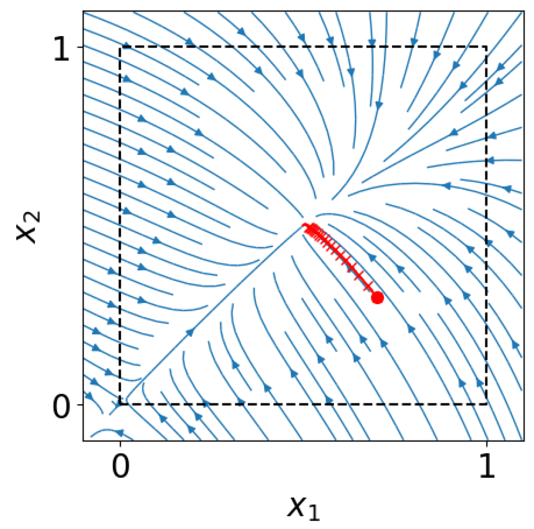
(d) $\operatorname{{\bf Interp}}\cap\operatorname{{\bf Inv}}\cap\operatorname{{\bf Mon}}$

Figure 6: Streamplots of polynomial vector fields of degree $2$ that are optimal to (16) with different side information constraints appended to it.

4.2 Dynamics of the simple pendulum

In this subsection, we consider the dynamics of the simple pendulum, i.e., a mass $m$ hanging from a massless rod of length $\ell$ (see Fig. 7). The state variables of this system are given by $x=(\theta,\dot{\theta})$, where $\theta$ is the angle that the rod makes with the vertical axis and $\dot{\theta}$ is the time derivative of this angle. By convention, the angle $\theta\in[-\pi,\pi]$ is positive when the mass is to the right of the vertical axis, and negative otherwise. By applying Newton’s second law of motion, the equation

$$\ddot{\theta}(t)=-\frac{g}{\ell}\sin(\theta(t))$$

for the dynamics of the pendulum can be derived, where $g$ here is the acceleration due to gravity. This is a one-dimensional second-order system that we convert to a first-order system as follows:

(18) $$\dot{x}(t)=f(x(t))\quad\text{where }\quad x(t)\coloneqq\begin{pmatrix}\theta(t)\\ \dot{\theta}(t)\end{pmatrix}\text{ and }f(\theta,\dot{\theta})\coloneqq\begin{pmatrix}\dot{\theta}\\ -\frac{g}{\ell}\sin\theta\end{pmatrix}.$$

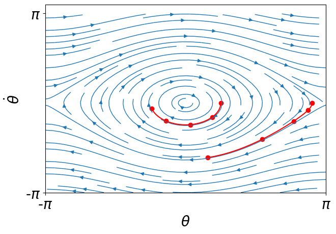
Figure 7: The simple pendulum and the streamplot of its vector field. We would like to learn this vector field over $[-\pi,\pi]^{2}$ from 10 noisy snapshots coming from two trajectories.

We take the vector field in (18) with $g=\ell=1$ to be the ground truth. We observe from this vector field a noisy version of two trajectories $x(t,x_{\text{init}}^{1})$ and $x(t,x_{\text{init}}^{2})$ sampled at times $t_{i}=\frac{3i}{5}$, where $i\in\{0,\ldots,4\}$, with $x_{\text{init}}^{1}=(\frac{\pi}{4},0)^{T}$ and $x_{\text{init}}^{2}=(\frac{9\pi}{10},0)^{T}$ (see Fig. 7). More precisely, we assume that our training set (with a slightly different representation of its elements) is given by

(19) $$\mathcal{D}\coloneqq\bigcup_{k=1}^{2}\left\{\begin{pmatrix}\theta(t_{i},x_{\text{init}}^{k})\\ \dot{\theta}(t_{i},x_{\text{init}}^{k})\\ \ddot{\theta}(t_{i},x_{\text{init}}^{k})\end{pmatrix}+10^{-2}\varepsilon_{i,k}\right\}_{i=0}^{4},$$

where the $\varepsilon_{i,k}$ (for $k=1,2$ and $i=0,\ldots,4$) are independent $3\times 1$ standard normal vectors.

We are interested in learning the vector field $f$ over the set $\Omega\coloneqq[-\pi,\pi]^{2}$ from the training data in (19). We parameterize our candidate vector field $p:\mathbb{R}^{2}\rightarrow\mathbb{R}^{2}$ as a $\text{degree-}5$ polynomial. Note that $p_{1}(\theta,\dot{\theta})=\dot{\theta}$, just from the meaning of our state variables. The only unknown is therefore the polynomial $p_{2}(\theta,\dot{\theta})$.

In absence of side information, one can solve a least-squares problem that finds a polynomial of degree $5$ that best agrees with the training data. As it can be seen in Fig. 8(a), the resulting vector field is very far from the true vector field and is unable to even replicate the observed trajectories when started from the same two initial conditions. To learn a better model, we describe a list of side information which could be derived from contextual knowledge without knowing the true vector field $f$.

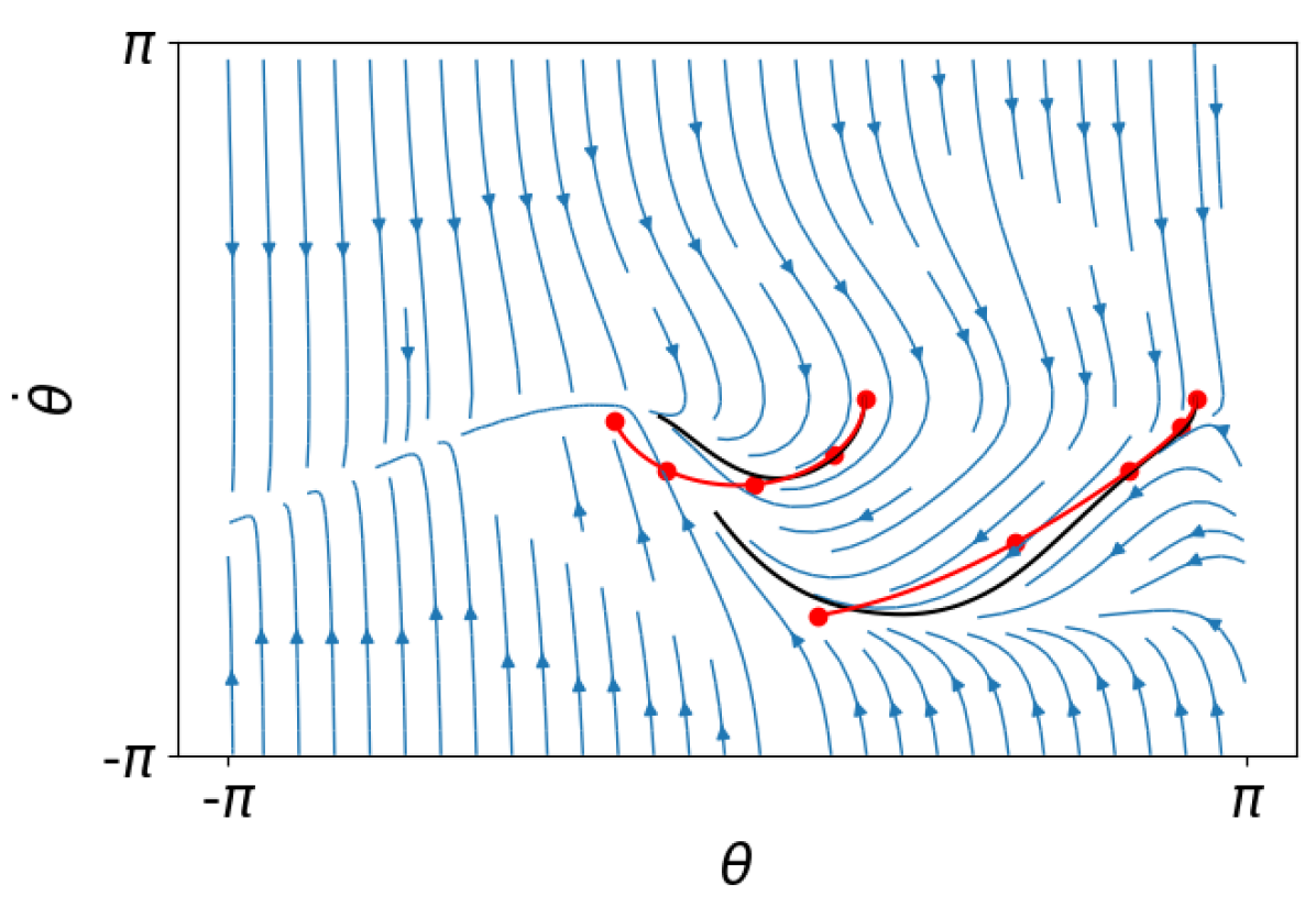
(a) No side information

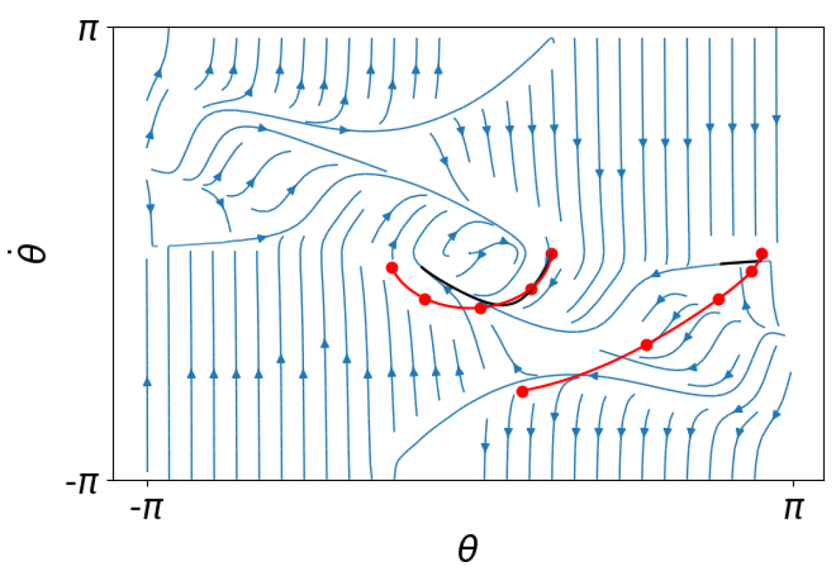
(b) $\operatorname{{\bf Sym}}$

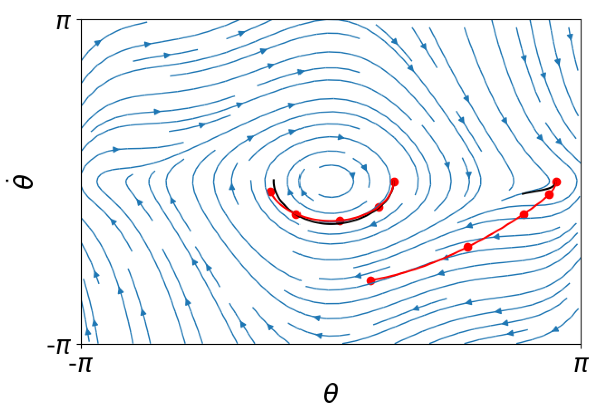
(c) $\operatorname{{\bf Sym}}\cap\operatorname{{\bf Pos}}$

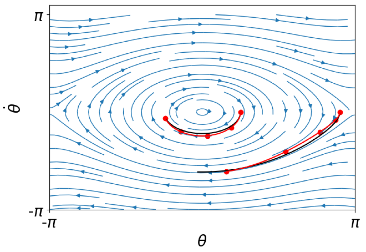
(d) $\operatorname{{\bf Sym}}\cap\operatorname{{\bf Pos}}\cap\operatorname{{\bf Ham}}$

Figure 8: Streamplots of polynomial vector fields of degree $5$ that best agree with the data (in the least-squares sense) and obey an increasing number of side information constraints. In each case, the trajectories of the learned vector field starting from the same two initial conditions as the trajectories observed in the training set are plotted in black.

Figure 9: Comparison of the trajectory of the simple pendulum in (18) starting from $(\frac{\pi}{4},0)^{T}$ (dotted) with the trajectory from the same initial condition of the polynomial vector field of degree 5 that best agrees with the data (in the least-squares solution) in the absence of side information (left), and subject to side information constraints $\operatorname{{\bf Sym}}\cap\operatorname{{\bf Pos}}\cap\operatorname{{\bf Ham}}$ (right).

• Sign symmetry ($\operatorname{{\bf Sym}}$). The pendulum obviously behaves symmetrically with respect to the vertical axis (plotted with a dotted line in Fig. 7). We therefore require our candidate vector field $p$ to satisfy the same symmetry condition

  $$p(-\theta,-\dot{\theta})=-p(\theta,\dot{\theta})\quad\forall(\theta,\dot{\theta})\in\Omega.$$

  Note that this is an affine constraint in the coefficients of the polynomial $p$, and that the true vector field $f$ in (18) satisfies this constraint.

• Coordinate nonnegativity ($\operatorname{{\bf Pos}}$). We know that the force of gravity pulls the pendulum’s mass down and pushes the angle $\theta$ towards $0$. This means that the angular velocity $\dot{\theta}$ decreases when $\theta$ is positive and increases when $\theta$ is negative. Mathematically, we must have

  $$p_{2}(\theta,\dot{\theta})\leq 0\;\forall(\theta,\dot{\theta})\in[0,\pi]\times[-\pi,\pi]\text{ and }p_{2}(\theta,\dot{\theta})\geq 0\;\forall(\theta,\dot{\theta})\in[-\pi,0]\times[-\pi,\pi].$$

  We replace each one of these constraints with their corresponding $\text{degree-}4$ sos certificate (see the definition following equation (11)). (Note that, because of the previous symmetry side information, we actually only need to impose one of these two constraints.)

• Hamiltonian ($\operatorname{{\bf Ham}}$). In the simple pendulum model, there is no dissipation of energy (through friction for example), so the total energy

  (20) $$E(\theta,\dot{\theta})=\frac{1}{2}ml^{2}{\dot{\theta}}^{2}+mgl(1-\cos(\theta))$$

  is conserved. The two terms appearing in this equation can be interpreted physically as the kinetic and the potential energy of the system. Furthermore, the total energy $E$ satisfies

  $$\dot{\theta}(t)=\frac{1}{m\ell^{2}}\frac{\partial E}{\partial\dot{\theta}}(\theta(t),\dot{\theta}(t)),\text{ and }\ddot{\theta}(t)=-\frac{1}{m\ell^{2}}\frac{\partial E}{\partial\theta}(\theta(t),\dot{\theta}(t)).$$

  The simple pendulum system is therefore a Hamiltonian system, with the associated Hamiltonian function $\frac{E}{m\ell^{2}}$. Note that neither the vector field in (18) describing the dynamics of the simple pendulum nor the associated Hamiltonian are polynomial functions. In our learning procedure, we use only the fact that the system is Hamiltonian, i.e., that there exists a function $H$ such that

  (21) $$p_{1}(\theta,\dot{\theta})=\frac{\partial H}{\partial\dot{\theta}}(\theta,\dot{\theta}),\text{ and }p_{2}(\theta,\dot{\theta})=-\frac{\partial H}{\partial\theta}(\theta,\dot{\theta}),$$

  but not the exact form of this Hamiltonian. Since we are parameterizing the candidate vector field $p$ as a $\text{degree-}5$ polynomial, the function $H$ must be a (scalar-valued) polynomial of degree $6$. The Hamiltonian structure can thus be imposed by adding affine constraints on the coefficients of $p$, or by directly learning $H$ and obtaining $p$ from (21).

Observe from Fig. 8 that as more side information is added, the behavior of the learned vector field gets closer to the truth. In particular, the solution returned by our semidefinite program in Fig. 8(d) is almost identical to the true dynamics in Fig. 7 even though it is obtained only from $10$ noisy samples on two trajectories. Fig. 9 shows that even if we start from an initial condition from which we have made partial trajectory observations, using side information can lead to better predictions for the future of the trajectory.

4.3 Growth of cancerous tumor cells

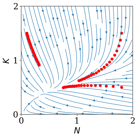
Figure 10: Streamplot of the vector field in Eq. 23 describing the time evolution of the volume $N$ of a cancerous tumor and the host’s carrying capacity $K$ (in cubic centimeters). We consider this vector field to be the ground truth and unkown to us. We try to learn it over $[0,2]^{2}$ from noisy measurements of three trajectories (plotted in red).

In this subsection, we consider a model governing the time evolution of the volume $N$ of a cancerous tumor inside a human body [43]. Cancerous tumors depend for their development on availability of the so-called Endothelial cells, the supply of which is characterized by a quantity called the carrying capacity $K$. Intuitively, $K$, which has the same unit as $N$, is proportional to the physical and energetic resources available for cell growth.

Two common modeling assumptions in cancer cell biology are that (i) the growth rate of the tumor decreases as the tumor grows, and (ii) that the volume of the tumor increases (resp. decreases) if it is below (resp. above) the carrying capacity. We follow the dynamics proposed in [43], which in contrast to prior works in that literature, also models the time evolution of the carrying capacity. The dynamics reads

(22) $$\begin{pmatrix}\dot{N}(t)\\ \dot{K}(t)\end{pmatrix}=f(N(t),K(t)),$$

where $f:\mathbb{R}^{2}\rightarrow\mathbb{R}^{2}$ is given by

(23) $$f_{1}(N,K)\coloneqq\frac{\mu N}{\nu}\left[1-\left(\frac{N}{K}\right)^{\nu}\right],\quad f_{2}(N,K)\coloneqq\omega N-\gamma N^{\frac{2}{3}}K.$$

Here, $\mu,\nu,\gamma$ and $\omega$ are positive parameters. The dynamics of $N$ is motivated by the so-called generalized logistic differential equation; the term $\omega N$ models the influence of the tumor on the Endothelial cells via short-range stimulators, and the term $-\gamma N^{\frac{2}{3}}K$ models this same influence via long-range inhibitors. See [43] for more details.

Having an accurate model of the growth dyanmics of cancerous tumors is crucial for the follow-up task of designing treatment plans, e.g., via radiation therapy. We hope that in the future leveraging side information can lead to learning more accurate models directly from patient data (as opposed to postulating an exact functional form such as (23)). For the moment however, we take (23) with the following parameters to be the ground truth:

$$(\mu,\nu,\gamma,\omega)=\frac{1}{10}(1,5,1,2).$$

See Fig. 10 for a streamplot of the corresponding vector field.

We consider the task of learning the vector field $f$ over the compact set $\Omega\coloneqq[0,2]^{2}$ from noisy snapshots of three trajectories. Each trajectory was started from a random initial conditions $x_{\text{init}}^{k}\coloneqq(N_{\text{init}}^{k},K_{\text{init}}^{k})$ (with $k=1,2,3$) inside $\Omega$ and sampled at times $t_{i}=i/{20}$, with $i=0,\ldots,19$ (see Fig. 10). More precisely, we have access to the following training data:

(24) $$\scriptsize\mathcal{D}\coloneqq\left\{\left((N(t_{i},x_{\text{init}}^{k}),K(t_{i},x_{\text{init}}^{k})),(\dot{N}(t_{i},x_{\text{init}}^{k})+10^{-4}\varepsilon_{i,k,1},\dot{K}(t_{i},x_{\text{init}}^{k})+10^{-4}\varepsilon_{i,k,2})\right)\right\}_{0\leq i<20,1\leq k\leq 3},$$

where the $\varepsilon_{i,k,l}$ (for $i=0,\ldots,19$, $k=1,\ldots,3$, and $l=1,2$) are independent standard normal variables. We parameterize our candidate vector field $p$ as a $\text{degree-}5$ polynomial. Without any side infromation, fitting this candidate vector field to the data in Eq. 24 via a least-squares problem leads to the vector field plotted in Fig. 11(a). Once again, the vector field obtained in this way is very far from the true vector field.

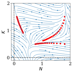
(a) No side information

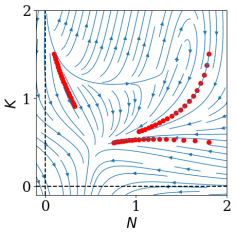
(b) $\operatorname{{\bf Pos}}\text{-}\operatorname{{\bf Mon}}$

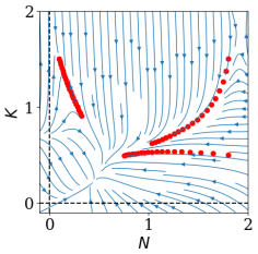
(c) $\operatorname{{\bf Pos}}\text{-}\operatorname{{\bf Mon}}\cap\operatorname{{\bf Inv}}$

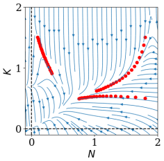
(d) $\operatorname{{\bf Pos}}\text{-}\operatorname{{\bf Mon}}\cap\operatorname{{\bf Inv}}\cap\operatorname{{\bf Pos}}$

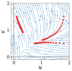
(e) $\operatorname{{\bf Pos}}\text{-}\operatorname{{\bf Mon}}\cap\operatorname{{\bf Inv}}\cap\operatorname{{\bf Pos}}$
$\cap\operatorname{{\bf Interp}}$

Figure 11: Streamplots of polynomial vector fields of degree $5$ that best agree with the data (in the least-squares sense) and obey an increasing number of side information constraints.

To do a better job at learning, we impose the side information constraints listed below that come from expert knowledge in the tumor growth literature (see, e.g., [43, 48, 24]):

• A mix between coordinate nonnegativity and coordinate directional monotonicity ($\operatorname{{\bf Pos}}\text{-}\operatorname{{\bf Mon}}$). As stated in [43], “one of the few near-universal observations about solid tumors is that almost all decelerate, i.e., reduce their specific growth rate $\frac{\dot{N}}{N}$, as they grow larger.”

  Based on this contextual knowledge, our candidate vector field $p$ should satisfy

  $$\frac{1}{N}\frac{\partial p_{1}}{\partial N}(N,K)-\frac{1}{N^{2}}p_{1}(N,K)\leq 0\quad\forall N\in(0,2],\;\forall K\in[0,2].$$

  Since the state variable $N$ is nonnegative at all times, we can clear denominators to obtain the constraint

  $$N\frac{{\partial}p_{1}}{{\partial}N}(N,K)-p_{1}(N,K)\leq 0\;\forall(N,K)\in[0,2]^{2}.$$

  This is a polynomial nonnegativity constraint over a closed basic semialgebraic set.

• Invariance of the nonnegative orthant ($\operatorname{{\bf Inv}}$). The state variables $N$ and $K$ quantify volumes, and as such, should be nonnegative at all times. This corresponds to the nonnegativity constraints

  $$p_{2}(N,0)\geq 0\;\forall N\in[0,2],\quad p_{1}(0,K)\geq 0\;\forall K\in[0,2].$$

• Coordinate nonnegativity ($\operatorname{{\bf Pos}}$). As mentioned before, the rate of change $\dot{N}$ in the tumor volume is nonnegative when the carrying capacity $K$ exceeds $N$, and nonpositive otherwise [43]. Mathematically, we must have

  $$p_{1}(N,K)\geq 0\quad\forall N\in[0,2],\;\forall K\in[N,2],$$

  $$p_{1}(N,K)\leq 0\quad\forall N\in[0,2],\;\forall K\in[0,N].$$

• Equilibrium point at the origin ($\operatorname{{\bf Interp}}$). The tumor does not grow if the volume of cancerous cells and the carrying capacity are both zero. This corresponds to the constraint $p(0,0)=0$.

We observe from Fig. 11 that as more side information is added, the behavior of the learned vector field gets closer and closer to the ground truth. In particular, the solution returned by our semidefinite program in Fig. 11(e) is very close to the true dynamics in Fig. 10.

4.4 Learning the Lorenz system

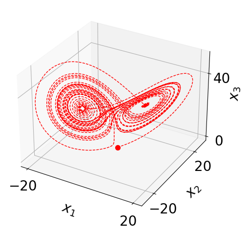
Figure 12: Sample trajectory of the system in (25) starting from $x(0)=(1,1,1)^{T}$.

In this subsection, we consider the classical Lorenz system (see, e.g., [50]) that is known for the chaotic properties of its solutions:

(25) $$\dot{x}(t)=f(x(t)),\text{where}\;x(t)\in\mathbb{R}^{3}\text{ and }f(x)=\left(\begin{array}[]{l}\sigma(x_{2}-x_{1})\\ x_{1}(\rho-x_{3})-x_{2}\\ x_{1}x_{2}-\beta x_{3}\end{array}\right).$$

Here, we work with the commonly used parameter values

$$\rho=2,\sigma=10,\text{ and }\beta=\frac{8}{3}.$$

We consider the task of learning the Lorenz system in (25) from 20 noisy snapshots of $N_{t}$ trajectories. More precisely, our data is $\mathcal{D}^{1}\cup\ldots\cup\mathcal{D}^{N_{t}}$, where for $k=1,\ldots,N_{t}$,

(26) $$\mathcal{D}^{k}\coloneqq\left\{\left(x(t_{i},x_{\text{init}}^{k}),f(x(t_{i},x_{\text{init}}^{k}))+10^{-1}\begin{pmatrix}\varepsilon^{k}_{i,1}\\ \varepsilon^{k}_{i,2}\\ \varepsilon^{k}_{i,3}\end{pmatrix}\right)\right\}_{i=1}^{20}.$$

Here, $x_{\text{init}}^{k}$ is generated uniformly at random from the box $[0,10]^{3}$, and the scalars $\varepsilon^{k}_{i,l}$ (for $i=1,\ldots,20$, and $l=1,\ldots,3$) are independent standard normal variables. We parameterize our candidate vector field $p:\mathbb{R}^{3}\rightarrow\mathbb{R}^{3}$ as a polynomial of degree $3$. The degree is taken to be larger than $2$ because we do not want to assume knowledge of the degree of the true vector field in Eq. 25. We assume access to the following list of side information:

• Equilibrium point at the origin ($\operatorname{{\bf Interp}}$). This corresponds to the constraint $p(0)~{}=~{}0$.

• Coordinate nonnegativity ($\operatorname{{\bf Pos}}$). The state variable $x_{1}$ should increase when $x_{2}~{}\geq~{}x_{1}$ and decrease otherwise. In other words,

  $$p_{1}(x)\geq 0\;\forall x\in S,\quad p_{1}(x)\leq 0\;\forall x\in S^{\prime},$$

  where $S\coloneqq\{x\in\mathbb{R}^{3}\;|\;x_{2}-x_{1}\geq 0\}$ and $S^{\prime}\coloneqq\{x\in\mathbb{R}^{3}\;|\;x_{2}-x_{1}\leq 0\}.$

• Monotonicity ($\operatorname{{\bf Mon}}$). The rate of change of any state variable decreases as the variable gets larger. In other words,

  $$\frac{\partial p_{i}}{\partial x_{i}}(x)\leq 0\quad\forall x\in\mathbb{R}^{3},\quad i=1,2,3.$$

Since a 3-dimensional streamplot is too clutered to be insightful, we instead report in Table 1 the test error of the polynomial vector field of degree $d=3$ learned from the side information and the data described above. Here, the test error of the vector field $p$ is measured as

$$\frac{1}{1000}\sum_{x\in D}\|p(x)-f(x)\|,$$

where $D$ is a uniform discretization of the box $[-10,10]^{3}$ with 1000 samples. As one can observe, the test error is reduced most of the time as more side information constraints are incorporated. For experiments with other degrees, noise levels, and a different notion of test error, see the appendix.

Side information:	$\emptyset$	$\operatorname{{\bf Interp}}$	$\operatorname{{\bf Interp}}\cap\operatorname{{\bf Pos}}$	$\operatorname{{\bf Interp}}\cap\operatorname{{\bf Pos}}\cap\operatorname{{\bf Mon}}$
$N_{t}=1$	1.47e+03	516	664	54.9
$N_{t}=2$	4.61	2.51	2.25	0.963
$N_{t}=3$	1.38	0.943	0.787	0.352

Table 1: Test error of cubic vector fields learned from side information and noisy snapshots of $N_{t}$ trajectories of the Lorenz system.

4.5 Following learning with optimal control

In this subsection, we revisit the contagion dynamics (13) and study the effect of side information on policy decisions to contain an outbreak. Suppose that by an initial screening of a random subset of the population, it is estimated that a fraction $0.5$ (resp. $0.4$) of males (resp. females) are infected with the disease. We would like to contain the outbreak by performing daily widespread testing of the population. We introduce two control decision variables $u_{1}$ and $u_{2}$, representing respectively the fraction of the population of males and females that are tested per unit of time. We suppose that testing slows down the spread of the disease (due e.g. to appropriate action that can be taken on the positive cases) as follows:

(27) $$\dot{x}(t)=f(x(t))-\begin{pmatrix}u_{1}x_{1}\\ u_{2}x_{2}\end{pmatrix},$$

where $f(x(t))$ is the unknown dynamics of the spread of the disease in the absence of any control.

We suppose that the monetary cost of testing a fraction $u_{1}$ of males and $u_{2}$ of females is given by $\alpha(u_{1}+u_{2})$ for some known positive scalar $\alpha$. Our goal is to minimize the sum

(28) $$c(u_{1},u_{2})\coloneqq x_{1}(T,\hat{x}_{\text{init}})+x_{2}(T,\hat{x}_{\text{init}})+\alpha(u_{1}+u_{2}),$$

of the total number $x_{1}(T,\hat{x}_{\text{init}})+x_{2}(T,\hat{x}_{\text{init}})$ of infected individuals at the end of a desired time period $T$, and the monetary cost $\alpha(u_{1}+u_{2})$ of our control law. Here, $x_{1}(t,\hat{x}_{\text{init}})$ and $x_{2}(t,\hat{x}_{\text{init}})$ evolve according to (27) when started from the point $\hat{x}_{\text{init}}=(0.5,0.4)^{T}$. In our experiments, we take $T=20$, $\alpha=0.4$, and $f$ to be the vector field in (13) with parameters in (14).

Given access to the vector field $f$, one could simply design an optimal control law $(u_{1}^{*},u_{2}^{*})$ that minimizes the cost function $c(u_{1},u_{2})$ in (28) by gridding the control space $[0,1]^{2}$, and computing $c(u_{1},u_{2})$ for every point of the grid. Indeed, for a given $(u_{1},u_{2})$, $c(u_{1},u_{2})$ can be computed by simulating the dynamics in (27) from the initial condition $\hat{x}_{\text{init}}$. The optimal control law obtained by following this strategy is depicted in Figure 13 together with the graph of the function $c(u_{1},u_{2})$.

We now consider the same setup as Section 4.1, where we do not know the vector field $f$, but have observed $20$ noisy samples of a single trajectory of it starting from $(0.7,0.3)^{T}$ (c.f. (15)). We design our control laws instead for the four polynomial vector fields of degree $3$ that were learned in Section 4.1 with no side information, with $\operatorname{{\bf Interp}}$, with $\operatorname{{\bf Interp}}\cap\operatorname{{\bf Inv}}$, and with $\operatorname{{\bf Interp}}\cap\operatorname{{\bf Inv}}\cap\operatorname{{\bf Mon}}$. This is done by following the procedure described in the previous paragraph, but using the learned vector field instead of $f$. The corresponding four control laws are depicted in Figure 13 with black arrows. We emphasize that while the control laws are computed from the learned vector fields, their associated costs in Figure 13 are computed by applying them to the true vector field. It is interesting to observe that adding side information constraints during the learning phase leads to the design of better control laws.

From Table 2, we see that if we had access to the true vector field, an optimal control law would lead to the eradication of the disease by time $T$. The first four rows of this table demonstrate the fraction of infected males and females at time $T$ when control laws that are optimal for dynamics learned with different side information constraints are applied to the true vector field. It is interesting to note that with no side information, a large fraction of the population remains infected, whereas control laws computed with three side information constraints are able to eradicate the disease almost completely.

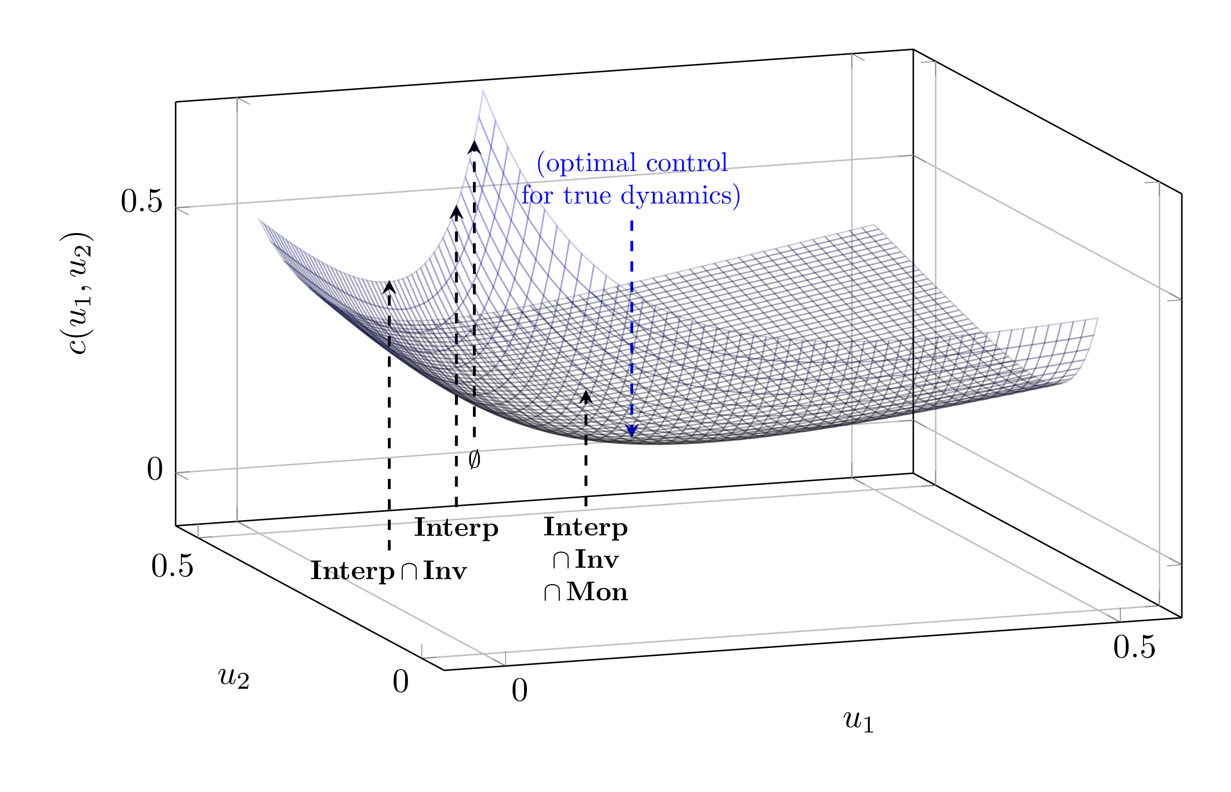
Figure 13: The graph of the function $c(u_{1},u_{2})$ in (28) with $T~{}=~{}20$, $\alpha=0.4$, and $f$ as in (13) with parameters in (14). The minimizer of the function $c(u_{1},u_{2})$, which corresponds to the optimal control law, is indicated with a blue arrow. The control laws that are optimal for dynamics learned from a single trajectory of $f$ with different side information constraints are indicated with black arrows.

Side information	$x_{1}(T,\hat{x}_{\text{init}})$	$x_{2}(T,\hat{x}_{\text{init}})$
None	0.45	0.40
$\operatorname{{\bf Interp}}$	0.41	0.29
$\operatorname{{\bf Interp}}\cap\operatorname{{\bf Inv}}$	0.31	0.12
$\operatorname{{\bf Interp}}\cap\operatorname{{\bf Inv}}\cap\operatorname{{\bf Mon}}$	0.01	0.01
True vector field	0.00	0.00

Table 2: The first four rows indicate the fraction of infected males and females at the end of the period $T$ when a control law, optimal for dynamics learned from a single trajectory with different side information constraints, is applied to the true vector field. The last row indicates the fraction of infected males and females at time $T$ resulting from applying the optimal control law computed with access to the true dynamics.

5 Approximation Results

In this section, we present some density results for polynomial vector fields that obey side information. This provides some theoretical justification for our choice of parameterizing our candidate vector fields as polynomial functions.

More precisely, we are interested in the following question: Given a continuously-differentiable vector field $f$ satisfying a list of side information constraints from Section 2, is there a polynomial vector field that is “close” to $f$ and satisfies the same list of side information constraints? For the purpose of learning dynamical systems, arguably the most relevant notion of “closeness” between two vector fields is one that measures how differently their corresponding trajectories can behave when started from the same initial condition. More formally, we fix a compact set $\Omega\subset\mathbb{R}^{n}$ and a time horizon $T$, and we define the following notion of distance between any two vector fields $f,g\in{C_{1}^{\circ}(\Omega)}$:

(29) $$d_{\Omega,T}(f,g)\coloneqq\sup_{(t,x_{\text{init}})\in\mathcal{S}}\max\left\{\|x_{f}(t,x_{\text{init}})-x_{g}(t,x_{\text{init}})\|_{2},\|\dot{x}_{f}(t,x_{\text{init}})-\dot{x}_{g}(t,x_{\text{init}})\|_{2}\right\},$$

where $x_{f}(t,x_{\text{init}})$ (resp. $x_{g}(t,x_{\text{init}})$) is the trajectory starting from $x_{\text{init}}\in\Omega$ and following the dynamics of $f$ (resp. $g$), and

(30) $$\mathcal{S}\coloneqq\{(t,x_{\text{init}})\in[0,T]\times\Omega\;|\;x_{f}(s,x_{\text{init}}),x_{g}(s,x_{\text{init}})\in\Omega\;\forall s\in[0,t]\}.$$

The reason why in the definition of $d_{\Omega,T}$, we take the supremum over $\mathcal{S}$ instead of over $[0,T]\times\Omega$ is to ensure that the trajectories that appear in (29) are well defined.

In Section 5.1, we show that under some assumptions that are often met in practice, polynomial vector fields can be made arbitrarily close to any continuously-differentiable vector field $f$ (in the sense of (29)), even if they are required to satisfy one side information constraint that $f$ is known to satisfy. In Section 5.2, we drop our assumptions and generalize this approximation result to any list of side information constraints at the price of allowing an arbitrarily small error in the satisfaction of these constraints. Furthermore, we show that the approximate satisfaction of side information can be certified by a sum of squares proof.

5.1 Approximating a vector field while (exactly) satisfying one side information constraint

The following theorem is the main result of this section. We will need the following definition for a subcase of this theorem: Given a collection of sets $A_{1},\ldots,A_{r}$, we define $\mathcal{G}(A_{1},\ldots,A_{r})$ to be the graph on $r$ vertices labeled by the sets $A_{1},\ldots,A_{r}$, where two vertices $A_{i}$ and $A_{j}$ are connected if $A_{i}\cap A_{j}\neq\emptyset$.

Theorem 5.1.

For any compact set $\Omega\subset\mathbb{R}^{n}$, time horizon $T>0$, desired accuracy $\varepsilon>0$, and vector field $f\in{C_{1}^{\circ}(\Omega)}$ which satisfies one of the following side information constraints (see Section 2):

1. $\operatorname{{\bf Interp}}(\{(x_{i},y_{i})\}_{i=1}^{m})$, where $x_{1},\ldots,x_{m}\in\Omega$,

2. $\operatorname{{\bf Sym}}(G,\sigma,\rho)$,

3. $\operatorname{{\bf Pos}}(\{(P_{i},N_{i})\}_{i=1}^{n})$, where for each $i\in\{1,\ldots,n\}$, $P_{i}\cap N_{i}=\emptyset$,

4. $\operatorname{{\bf Mon}}(\{(P_{ij},N_{ij})\}_{i,j=1}^{n})$, where for each $i,j\in\{1,\ldots,n\}$, the sets $P_{ij}$ and $N_{ij}$ belong to different connected components of the graph $\mathcal{G}(P_{i1},N_{i1},\ldots,P_{in},N_{in})$,

5. $\operatorname{{\bf Inv}}(\{B_{i}\}_{i=1}^{r})$, where the sets $B_{i}$ are pairwise nonintersecting, and defined as $B_{i}\coloneqq\{x\in\mathbb{R}^{n}\;|\;h_{ij}(x)\geq 0,\;j=1,\dots,m_{i}\}$ for some concave continuously-differentiable functions $h_{ij}$ that satisfy

   $$\forall i\in\{1,\ldots,r\},\;\exists x^{i}\in B_{i}\text{ such that }h_{ij}(x^{i})>0\text{ for }j=1,\ldots,m_{i},$$

6. $\operatorname{{\bf Grad}}$,

7. $\operatorname{{\bf Ham}}$,

there exists a polynomial vector field $p:\mathbb{R}^{n}\rightarrow\mathbb{R}^{n}$ that satisfies the same side information constraint as $f$ and has $d_{\Omega,T}(f,p)\leq\varepsilon.$

Before we present the proof, we recall the classical Stone-Weierstrass approximation theorem. Note that while the theorem is stated here for scalar-valued functions, it readily extends to vector-valued ones.

Theorem 5.2.

(see, e.g., [51]) For any compact set $\Omega\subset\mathbb{R}^{n}$, scalar $\varepsilon>0$, and continuous function $f:\Omega\rightarrow\mathbb{R}$, there exists a polynomial $p:\mathbb{R}^{n}\rightarrow\mathbb{R}$ such that

$$\max_{x\in\Omega}|f(x)-p(x)|\leq\varepsilon.$$

For two vector fields $f,g:\mathbb{R}^{n}\rightarrow\mathbb{R}^{n}$ and a set $\Omega\subseteq\mathbb{R}^{n}$, let us define

$$\|f-g\|_{\Omega}\coloneqq\max_{x\in\Omega}\|f(x)-g(x)\|_{2}.$$

The following proposition relates this quantity to the notion of distance $d_{\Omega,T}(f,g)$ defined in (29). We recall that for a scalar $L\geq 0$, a vector field $f$ is said to be $L\text{-Lipschitz}$ over $\Omega$ if

$$\|f(x)-f(y)\|_{2}\leq L\|x-y\|_{2}\quad\forall x,y\in\Omega.$$

Note that any vector field $f\in{C_{1}^{\circ}(\Omega)}$ is $L\text{-Lipschitz}$ over a compact set $\Omega$ for some nonnegative scalar $L$.

Proposition 5.3.

For any compact set $\Omega\subset\mathbb{R}^{n}$, any finite time horizon $T>0$, and any two vector fields $f,g\in{C_{1}^{\circ}(\Omega)}$, we have

$$\|f-g\|_{\Omega}\leq d_{\Omega,T}(f,g)\leq\max\{Te^{LT},1+LTe^{LT}\}\|f-g\|_{\Omega},$$

where $L\geq 0$ is any scalar for which either $f$ or $g$ is $L\text{-Lipschitz}$ over $\Omega$.

We note that the dependence of the right-most term on $T$ cannot be avoided. (For example, for $n=1$, $\Omega=[0,1]$, $f(x)=0$, $g_{\varepsilon}(x)=\varepsilon x$, we have $\|f-g_{\varepsilon}\|_{\Omega}=\varepsilon$, but $d_{\Omega,T}(f,g_{\varepsilon})\geq\frac{1}{2}$ for all $T\geq\frac{\log 2}{\varepsilon}$.) To present the proof of this proposition, we need to recall the Grönwall-Bellman inequality.

Lemma 5.4 (Grönwall-Bellman inequality [6, 27]).

Let $I=[a,b]$ denote a nonempty interval on the real line. Let $u$, $\alpha$, $\beta:I\rightarrow\mathbb{R}$ be continuous functions satisfying

$$u(t)\leq\alpha(t)+\int_{a}^{t}\beta(s)u(s)\;{\rm d}s\quad\forall t\in I.$$

If $\alpha$ is nondecreasing and $\beta$ is nonnegative, then

$$u(t)\leq\alpha(t)e^{\int_{a}^{t}\beta(s)\;{\rm d}s}\quad\forall t\in I.$$

Proof 5.5 (Proof of Proposition 5.3).

We fix a compact set $\Omega\subset\mathbb{R}^{n}$, a time horizon $T>0$, and vector fields $f,g\in{C_{1}^{\circ}(\Omega)}$, with $f$ being $L\text{-Lipschitz}$ over $\Omega$ for some scalar $L\geq 0$. To see that the first inequality holds, note that for any $x_{\text{init}}\in\Omega$, $\dot{x}_{f}(0,x_{\text{init}})=f(x_{\text{init}})$ and $\dot{x}_{g}(0,x_{\text{init}})=g(x_{\text{init}})$. Therefore, $\|f-g\|_{\Omega}\leq d_{\Omega,T}(f,g)$.

For the second inequality, fix $(t,x_{\text{init}})\in\mathcal{S}$, where $\mathcal{S}$ is defined in (30). Let us first bound $\|x_{f}(t,x_{\text{init}})-x_{g}(t,x_{\text{init}})\|_{2}$. By definition of $x_{f}$ and $x_{g}$, we have

$$x_{f}(t,x_{\text{init}})-x_{g}(t,x_{\text{init}}) =\int_{0}^{t}f(x_{f}(s,x_{\text{init}}))-g(x_{g}(s,x_{\text{init}})){\rm d}s$$

$$=\int_{0}^{t}f(x_{f}(s,x_{\text{init}}))-f(x_{g}(s,x_{\text{init}}))\;{\rm d}s$$

$$+\int_{0}^{t}f(x_{g}(s,x_{\text{init}}))-g(x_{g}(s,x_{\text{init}}))\;{\rm d}s.$$

Using the triangular inequality, we get

(31) $$\begin{split}\|x_{f}(t,x_{\text{init}})-x_{g}(t,x_{\text{init}})\|_{2}&\leq\int_{0}^{t}\|f(x_{f}(s,x_{\text{init}}))-f(x_{g}(s,x_{\text{init}}))\|_{2}\;{\rm d}s\\ &+\int_{0}^{t}\|f(x_{g}(s,x_{\text{init}}))-g(x_{g}(s,x_{\text{init}}))\|_{2}\;{\rm d}s.\end{split}$$

Because the function $f$ is $L\text{-Lipschitz}$ over $\Omega$, we have

$$\|f(x_{f}(s,x_{\text{init}}))-f(x_{g}(s,x_{\text{init}}))\|_{2}\leq L\|x_{f}(s,x_{\text{init}})-x_{g}(s,x_{\text{init}})\|_{2}\quad\forall s\in[0,t].$$

Furthermore, we know that for all $s\in[0,t]$, $x_{g}(s,x_{\text{init}})\in\Omega$, and therefore

$$\|f(x_{g}(s,x_{\text{init}}))-g(x_{g}(s,x_{\text{init}}))\|_{2}\leq\|f-g\|_{\Omega}.$$

We can hence further bound the left hand side of (31) as

$$\|x_{f}(t,x_{\text{init}})-x_{g}(t,x_{\text{init}})\|_{2} \leq L\int_{0}^{t}\|x_{f}(s,x_{\text{init}})-x_{g}(s,x_{\text{init}})\|_{2}\;{\rm d}s+t\|f-g\|_{\Omega}.$$

By Lemma 5.4, we get

(32) $$\|x_{f}(t,x_{\text{init}})-x_{g}(t,x_{\text{init}})\|_{2}\leq te^{Lt}\|f-g\|_{\Omega}.$$

Next, we bound the quantity$\|\dot{x}_{f}(t,x_{\text{init}})-\dot{x}_{g}(t,x_{\text{init}})\|_{2}$, which can be expressed in terms of the vector fields $f$ and $g$ as $\|f(x_{f}(t,x_{\text{init}}))-g(x_{g}(t,x_{\text{init}}))\|_{2}$. We have

(33) $$\begin{split}\|f(x_{f}(t,x_{\text{init}}))-g(x_{g}(t,x_{\text{init}}))\|_{2}&\leq\|f(x_{f}(t,x_{\text{init}}))-f(x_{g}(t,x_{\text{init}}))\|_{2}\\ &+\|f(x_{g}(t,x_{\text{init}}))-g(x_{g}(t,x_{\text{init}}))\|_{2}\\ &\leq L\|x_{f}(t,x_{\text{init}})-x_{g}(t,x_{\text{init}})\|_{2}+\|f-g\|_{\Omega}\\ &\leq(1+Lte^{Lt})\|f-g\|_{\Omega},\end{split}$$

where the first inequality follows from the triangular inequality, the second from the definition of $\|\cdot\|_{\Omega}$ and the fact that $f$ is $L\text{-Lipschitz}$ over $\Omega$, and the third one from (32).

Putting (32) and (33) together, and using the fact that $t\leq T$, we have

$$\max \left\{\|x_{f}(t,x_{\text{init}})-x_{g}(t,x_{\text{init}})\|_{2},\|f(x_{f}(t,x_{\text{init}}))-g(x_{g}(t,x_{\text{init}}))\|_{2}\right\}$$

$$\quad\quad\quad\quad\leq\max\{te^{Lt},1+Lte^{Lt}\}\|f-g\|_{\Omega}$$

$$\quad\quad\quad\quad\leq\max\{Te^{LT},1+LTe^{LT}\}\|f-g\|_{\Omega}.$$

Taking the supremum over $(t,x_{\text{init}})\in\mathcal{S}$, we get

$$d_{\Omega,T}(f,g)\leq\max\{Te^{LT},1+LTe^{LT}\}\|f-g\|_{\Omega}.$$

Proof 5.6 (Proof of Theorem 5.1).

Let us fix a compact set $\Omega\subset\mathbb{R}^{n}$, a time horizon $T>0$, and a desired accuracy $\varepsilon>0$. Let $f\in{C_{1}^{\circ}(\Omega)}$ be a vector field that satisfies any one of the side information constraints stated in the theorem. Note that $f$ is $L\text{-Lipschitz}$ over $\Omega$ for some $L\geq 0$. We claim that for any $\delta>0$, there exists a polynomial vector field $p:\mathbb{R}^{n}\rightarrow\mathbb{R}^{n}$ that satisfies the same side information constraint as $f$ and the inequality

$$\|f-p\|_{\Omega}\leq\delta.$$

By Proposition 5.3, if we take

(34) $$\delta=\varepsilon/\max\{Te^{LT},1+LTe^{LT}\},$$

this shows that there exists a polynomial vector field $p:\mathbb{R}^{n}\rightarrow\mathbb{R}^{n}$ that satisfies the same side information as $f$ and the inequality

$$d_{\Omega,T}(f,p)\leq\varepsilon.$$

We now give a case-by-case proof of our claim above depending on which side information $f$ satisfies. Throughout the rest of the proof, the constant $\delta$ is fixed as in (34).

•  Case (i): Suppose $f\in\operatorname{{\bf Interp}}(\{(x_{i},y_{i})\}_{i=1}^{m})$, where $x_{1},\ldots,x_{m}\in\Omega$. Without loss of generality, we assume that the points $x_{i}$ are all different, or else we can discard the redundant constraints. Let $\delta^{\prime}$ be a positive constant that will be fixed later. By Theorem 5.2, there exists a polynomial vector field $q$ that satisfies $\|f-q\|_{\Omega}\leq\delta^{\prime}$. We claim that there exists a polynomial ${\tilde{q}}$ of degree $m-1$ such that

(35) $$(q+{\tilde{q}})(x_{i})=y_{i}\quad i=1,\ldots,m,$$

and $\|{\tilde{q}}\|_{\Omega}\leq C\delta^{\prime}$, where $C$ is a constant depending only on the points $x_{i}$ and the set $\Omega$. Indeed, (35) can be viewed as a linear system of equations where the unknowns are the coefficients of $\tilde{q}$ in some basis. For example, if we let $N={n+m-1\choose n}$ and ${\tilde{q}}_{\text{coeff}}\in\mathbb{R}^{N\times n}$ be the matrix whose $j\text{-th}$ column is the vector of coefficients of $\tilde{q}_{j}$ in the standard monomial basis, then (35) can be written as

(36) $$A\;{\tilde{q}}_{\text{coeff}}=\Delta,$$

where $\Delta\in\mathbb{R}^{m\times n}$ is the matrix whose $i\text{-th}$ row is given by $y_{i}^{T}-q(x_{i})^{T}$, and $A\in\mathbb{R}^{m\times N}$ is the matrix whose $i\text{-th}$ row is the vector of all standard monomials in $n$ variables and of degree up to $m-1$ evaluated at the point $x_{i}$. One can verify that the rows of the matrix $A$ are linearly independent (see, e.g., [15, Corollary 4.4]), and so the matrix $AA^{T}$ is invertible. If we let $A^{+}=A^{T}(AA^{T})^{-1}$, then ${\tilde{q}}_{\text{coeff}}=A^{+}\Delta$ is a solution to (36). Since the matrix $A^{+}$ only depends on the points $x_{i}$, and since all the entries of the matrix $\Delta$ are bounded in absolute value by $\delta^{\prime}$, there exists a constant $c$ such that all the entries of the matrix ${\tilde{q}}_{\text{coeff}}$ are bounded in absolute value by $c\delta^{\prime}$. Since the set $\Omega$ is compact, there exists a constant $C$ depending only on the points $x_{i}$ and the set $\Omega$ such that $\|{\tilde{q}}\|_{\Omega}\leq C\delta^{\prime}$.

Finally, by taking $p\coloneqq q+{\tilde{q}}$, we get $p\in\operatorname{{\bf Interp}}(\{(x_{i},y_{i})\}_{i=1}^{m}),$ and

$$\|f-p\|_{\Omega}\leq\delta^{\prime}(1+C).$$

We take $\delta^{\prime}=\frac{\delta}{1+C}$ to conclude the proof for this case.

•  Case (ii): Suppose $f\in\operatorname{{\bf Sym}}(G,\sigma,\rho)$, where $G$ is a finite group. Let $\delta^{\prime}$ be a positive constant that will be fixed later. By Theorem 5.2, there exists a polynomial vector field $p$ that satisfies $\|f-p\|_{\Omega}\leq\delta^{\prime}$. Let $p^{G}:\mathbb{R}^{n}\rightarrow\mathbb{R}^{n}$ be the polynomial defined as

$$p^{G}(x)\coloneqq\frac{1}{|G|}\sum_{g\in G}\rho(g^{-1})p(\sigma(g)x)\quad\forall x\in\mathbb{R}^{n},$$

where $|G|$ is the size of the group $G$. We claim that $p^{G}\in\operatorname{{\bf Sym}}(G,\sigma,\rho)$. Indeed, for any $h\in G$ and $x\in\Omega$, using the fact that $\sigma$ is a group homomorphism, we get

$$p^{G}(\sigma(h)x)=\frac{1}{|G|}\sum_{g\in G}\rho(g^{-1})p(\sigma(gh)x).$$

By doing the change of variables $g^{\prime}=gh$ in the sum above, and using the fact that $\rho$ is a group homomorphism, we get

$$p^{G}(\sigma(h)x) =\frac{1}{|G|}\sum_{g^{\prime}\in G}\rho(hg^{\prime-1})p(\sigma(g^{\prime})x)$$

$$=\frac{1}{|G|}\sum_{g^{\prime}\in G}\rho(h)\rho(g^{\prime-1})p(\sigma(g^{\prime})x).$$

$$=\rho(h)p^{G}(x).$$

We now claim that by by taking $\delta^{\prime}=\delta\left(\frac{1}{|G|}\sum_{g\in G}\|\rho(g^{-1})\|\right)^{-1}$, where $\|\cdot\|$ denotes the operator norm of its matrix argument, we get $\|f-p^{G}\|_{\Omega}\leq\delta$. Indeed,

$$f(x)-p^{G}(x) =\frac{1}{|G|}\sum_{g\in G}\left(f(x)-\rho(g^{-1})p(\sigma(g)x)\right)$$

$$=\frac{1}{|G|}\sum_{g\in G}\rho(g^{-1})\left(\rho(g)f(x)-p(\sigma(g)x)\right)$$

$$=\frac{1}{|G|}\sum_{g\in G}\rho(g^{-1})\left(f(\sigma(g)x)-p(\sigma(g)x)\right),$$

where in the last equation, we used the fact that $f\in\operatorname{{\bf Sym}}(G,\sigma,\rho)$. Therefore,

$$\|f(x)-p^{G}(x)\| \leq\frac{1}{|G|}\sum_{g\in G}\|\rho(g^{-1})\|\|f(\sigma(g)x)-p(\sigma(g)x)\|_{2}$$

$$\leq\left(\frac{1}{|G|}\sum_{g\in G}\|\rho(g^{-1})\|\right)\delta^{\prime}=\delta.$$

•  Case (iii): If $f\in\operatorname{{\bf Pos}}(\{(P_{i},N_{i})\}_{i=1}^{n})$, where for each $i\in\{1,\ldots,n\}$, the sets $P_{i}$ and $N_{i}$ are subsets of $\Omega$ and satisfy $P_{i}\cap N_{i}=\emptyset$.

For $i=1,\ldots,n$, let $d_{i}$ denote the distance between the sets $P_{i}$ and $N_{i}$:

$$d_{i}\coloneqq\min_{x\in P_{i},x^{\prime}\in N_{i}}\|x-x^{\prime}\|_{2}.$$

Since $P_{i}$ and $N_{i}$ are compact sets with empty intersection, the scalar $d_{i}$ is positive. Fix $\gamma$ to be any positive scalar smaller than $\min_{i=1,\ldots,n}d_{i}$. For $i=1,\ldots,n$, let

$$P_{i}^{\gamma}\coloneqq\{x+\frac{\gamma}{2}z\;|\;x\in P_{i},z\in\mathbb{R}^{n},\text{ and }\|z\|_{2}\leq 1\},$$

$$N_{i}^{\gamma}\coloneqq\{x+\frac{\gamma}{2}z\;|\;x\in N_{i},z\in\mathbb{R}^{n},\text{ and }\|z\|_{2}\leq 1\}.$$

With our choice of $\gamma$, $P_{i}^{\gamma}\cap N_{i}^{\gamma}=\emptyset\text{ for }i=1,\ldots,n.$ Let $\psi:\mathbb{R}^{n}\rightarrow\mathbb{R}^{n}$ be the piecewise-constant function defined as

$$\psi_{i}(x)=\left\{\begin{array}[]{cc}1&\text{if }x\in P_{i}^{\gamma}\\ -1&\text{if }x\in N_{i}^{\gamma}\\ 0&\text{otherwise}\end{array}\right.\quad\text{for }i=1,\ldots,n,$$

and $\phi^{\gamma}:\mathbb{R}^{n}\rightarrow\mathbb{R}$ be the “bump-like” function that is equal to $e^{-\frac{1}{1-\|z\|^{2}}}$ when $\|z\|_{2}\leq\frac{\gamma}{2}$ and $0$ elsewhere. Let $\psi^{\text{conv}}:\mathbb{R}^{n}\rightarrow\mathbb{R}^{n}$ be the normalized convolution of $\psi$ with $\phi^{\gamma}$ , i.e.,

$$\psi^{\text{conv}}(x)\coloneqq\frac{1}{\int_{z\in\mathbb{R}^{n}}\phi^{\gamma}(z){\rm d}z}\int_{z\in\mathbb{R}^{n}}\psi(x+z)\phi^{\gamma}(z){\rm d}z.$$

Note that $\psi^{\text{conv}}$ is a continuous function as it is the convolution of a piecewise-constant function $\psi$ with a continuous function $\phi^{\gamma}$. Moreover, for each $i\in\{1,\ldots,n\}$, $\psi^{\text{conv}}_{i}$ satisfies

$$\psi^{\text{conv}}_{i}(x)=1\;\forall x\in P_{i},\;\psi^{\text{conv}}_{i}(x)=-1\;\forall x\in N_{i},\;\text{and }|\psi^{\text{conv}}_{i}(x)|\leq 1\;\forall x\in\Omega.$$

Now let $f^{\delta}\in{C_{1}^{\circ}(\Omega)}$ be the vector field defined component-wise by

$$f^{\delta}_{i}(x)=f_{i}(x)+\frac{\delta}{2\sqrt{n}}\psi_{i}^{\text{conv}}(x)\quad i=1,\ldots,n.$$

Note that for $i=1,\ldots,n$, the function $f^{\delta}_{i}$ is continuous, bounded below by $\frac{\delta}{2\sqrt{n}}$ on $P_{i}$, and bounded above by $\frac{-\delta}{2\sqrt{n}}$ on $N_{i}$. Moreover $\|f-f^{\delta}\|_{\Omega}\leq\frac{\delta}{2}$. Theorem 5.2 guarantees the existence of a polynomial vector field $p$ such that $\|f^{\delta}-p\|_{\Omega}\leq\frac{\delta}{2\sqrt{n}}$. In particular, $p\in\operatorname{{\bf Pos}}(\{(P_{i},N_{i})\}_{i=1}^{n})$ and satisfies $\|f-p\|_{\Omega}\leq\delta$.

•  Case (iv): If $f\in\operatorname{{\bf Mon}}(\{(P_{ij},N_{ij})\}_{i,j=1}^{n})$, where for each $i,j\in\{1,\ldots,n\}$, the sets $P_{ij}$ and $N_{ij}$ are subsets of $\Omega$ and belong to different connected components of the graph $\mathcal{G}(P_{i1},N_{i1},\ldots,P_{in},N_{in})$. (Recall the definition of this graph from the first paragraph of Section 5.1.)

Consider an index $i\in\{1,\ldots,n\}$, and let $C_{i1},\ldots,C_{ir_{i}}$ be the connected components of the graph $\mathcal{G}(P_{i1},N_{i1},\ldots,P_{in},N_{in})$. Let $U_{il}$ be the union of the sets in component $C_{il}$. Since the sets $U_{i1},\ldots,U_{ir_{i}}$ are compact and pairwise non-intersecting, the minimum distance $d_{i}\coloneqq\min_{x\in U_{il},x^{\prime}\in U_{il^{\prime}},l\neq\l^{\prime}}\|x-x^{\prime}\|_{2}$ between any two of them is positive. Fix $\gamma_{i}$ to be a positive scalar smaller than $d_{i}$, and for each $l\in\{1,\ldots,r_{i}\}$, let

$$U_{il}^{\gamma_{i}}\coloneqq\{x+\frac{\gamma_{i}}{2}z\;|\;x\in U_{il},z\in\mathbb{R}^{n},\text{ and }\|z\|_{2}\leq 1\}.$$

Define $\psi_{i}:\mathbb{R}^{n}\rightarrow\mathbb{R}$ to be the piecewise-linear function defined as

$$\psi_{i}(x)=\left\{\begin{array}[]{cc}\sum_{j:P_{ij}\in C_{l}}x_{j}-\sum_{j:N_{ij}\in C_{l}}x_{j}&\text{if }x\in U_{il}^{\gamma_{i}}\text{ for some }l\in\{1,\ldots,r_{i}\}\\ 0&\text{otherwise.}\end{array}\right.$$

Let $\psi_{i}^{\text{conv}}:\mathbb{R}^{n}\rightarrow\mathbb{R}$ be the normalized convolution of $\psi_{i}$ with the “bump-like” function $\phi^{\gamma_{i}}:\mathbb{R}^{n}\rightarrow\mathbb{R}$ that is equal to $e^{-\frac{1}{1-\|z\|^{2}}}$ when $\|z\|_{2}\leq\frac{\gamma_{i}}{2}$ and $0$ elsewhere; that is

$$\psi_{i}^{\text{conv}}(x)\coloneqq\frac{1}{\int_{z\in\mathbb{R}^{n}}\phi^{\gamma_{i}}(z){\rm d}z}\int_{z\in\mathbb{R}^{n}}\psi_{i}(x+z)\phi^{\gamma_{i}}(z){\rm d}z.$$

The function $\psi_{i}^{\text{conv}}$ is continuously differentiable (because $\phi^{\gamma_{i}}$ is continuously differentiable) and satisfies

$$\frac{\partial\psi_{i}^{\text{conv}}}{\partial x_{j}}(x)=1\;\forall x\in P_{ij},\;\frac{\partial\psi_{i}^{\text{conv}}}{\partial x_{j}}(x)=-1\;\forall x\in N_{ij},$$

$$|\psi^{\text{conv}}_{i}(x)|\leq\sup_{x\in\Omega}|\psi_{i}(x)|\quad\forall x\in\Omega.$$

Now, let $\psi^{\text{conv}}\coloneqq(\psi^{\text{conv}}_{1},\ldots,\psi^{\text{conv}}_{n})^{T}$ and $f^{\delta^{\prime}}(x)\coloneqq f(x)+\delta^{\prime}\psi^{\text{conv}}(x)$ for a constant $\delta^{\prime}>0$ that will be fixed later. Note that $\|f^{\delta^{\prime}}-f\|_{\Omega}\leq\delta^{\prime}\|\psi^{\text{conv}}\|_{\Omega}$, and for each pair of indices $i,j\in\{1,\ldots,n\}$,

$$\frac{\partial f^{\delta^{\prime}}_{i}}{\partial x_{j}}(x)\geq\delta^{\prime}\;\forall x\in P_{ij},\;\frac{\partial f^{\delta^{\prime}}_{i}}{\partial x_{j}}(x)\leq-\delta^{\prime}\;\forall x\in N_{ij}.$$

A generalization of the Stone-Weierstrass approximation result stated in Theorem 5.2 to continuously-differentiable functions (see, e.g., [41]) guarantees the existence of a polynomial $p:\mathbb{R}^{n}\rightarrow\mathbb{R}^{n}$ such that

$$\|f^{\delta^{\prime}}-p\|_{\Omega}\leq\delta^{\prime},\quad\sup_{x\in\Omega}\left|\frac{\partial f_{i}^{\delta^{\prime}}}{\partial x_{j}}(x)-\frac{\partial p_{i}}{\partial x_{j}}(x)\right|\leq\delta^{\prime}/2\quad\forall i,j\in\{1,\ldots,n\}.$$

In particular, $p\in\operatorname{{\bf Mon}}(\{P_{ij},N_{ij}\}_{i,j=1}^{n})$ and satisfies $\|f-p\|_{\Omega}\leq\delta^{\prime}(1+\|\psi^{\text{conv}}\|_{\Omega})$. We conclude the proof by taking $\delta^{\prime}=\frac{\delta}{1+\|\psi^{\text{conv}}\|_{\Omega}}$.

•  Case (v): If $f\in\operatorname{{\bf Inv}}(\{B_{i}\}_{i=1}^{r})$, where the sets $B_{i}$ are subsets of $\Omega$, pairwise nonintersecting, and defined as $B_{i}\coloneqq\{x\in\mathbb{R}^{n}\;|\;h_{ij}(x)\geq 0,\;j=1,\dots,m_{i}\}$ for some continuously-differentiable concave functions $h_{ij}:\mathbb{R}^{n}\rightarrow\mathbb{R}$ that satisfy

(37) $$\forall i\in\{1,\ldots,r\},\;\exists x^{i}\in B_{i}\text{ such that }h_{ij}(x^{i})>0\text{ for }j=1,\ldots,m_{i}.$$

By the same argument as that for Case (iii), for each $i\in\{1,\ldots,r\}$, there exists a continuous function $\psi_{i}^{\text{conv}}:\mathbb{R}^{n}\rightarrow\mathbb{R}$ that satisfies

$$\psi_{i}^{\text{conv}}(x)=1\;\forall x\in B_{i},\psi_{i}^{\text{conv}}(x)=0\;\forall x\in\cup_{i^{\prime}\neq i}B_{i^{\prime}},\;|\psi_{i}^{\text{conv}}(x)|\leq 1\;\forall x\in\Omega.$$

Let $\delta^{\prime}\coloneqq\frac{\delta}{2r(1+\max_{x,x^{\prime}\in\Omega}\|x-x^{\prime}\|_{2})}$, and for $i=1\ldots,r$, let $x^{i}\in B_{i}$ be any point satisfying $h_{ij}(x^{i})>0\text{ for }j=1,\ldots,m_{i}$. Consider the continuous vector field

$$f^{\delta^{\prime}}(x)\coloneqq f(x)-\delta^{\prime}\sum_{i=1}^{r}\psi_{i}^{\text{conv}}(x)(x-x^{i}).$$

For every $x\in\Omega$, the triangular inequality gives

$$\|f(x)-f^{\delta^{\prime}}(x)\|_{2} \leq\delta^{\prime}\sum_{i=1}^{r}\|x-x^{i}\|_{2}$$

$$\leq r\delta^{\prime}\max_{x^{\prime}\in\Omega}\|x-x^{\prime}\|_{2}=\frac{\delta}{2},$$

and so $\|f-f^{\delta^{\prime}}\|_{\Omega}\leq\delta/2$. Furthermore, for each $i\in\{1,\ldots,r\}$, for each $j~{}\in~{}\{1,\ldots,m_{i}\}$, and for each $x\in B_{i}$ satisfying $h_{ij}(x)=0$,

(38) $$\langle f^{\delta^{\prime}}(x),\nabla h_{ij}(x)\rangle =\langle f(x),\nabla h_{ij}(x)\rangle-\delta^{\prime}\sum_{k=1}^{r}\phi_{k}^{\text{conv}}(x)\langle x-x^{k},\nabla h_{ij}(x)\rangle$$

$$=\langle f(x),\nabla h_{ij}(x)\rangle-\delta^{\prime}\langle x-x^{i},\nabla h_{ij}(x)\rangle$$

$$\geq-\delta^{\prime}\langle x-x^{i},\nabla h_{ij}(x)\rangle$$

$$\geq\delta^{\prime}(h_{ij}(x^{i})-h_{ij}(x))$$

$$=\delta^{\prime}h_{ij}(x^{i}),$$

where the second equality follows from the definition of $\psi_{i}^{\text{conv}}$ and the fact that $x\in B_{i}$, the first inequality from the fact that$f\in\operatorname{{\bf Inv}}(\{B_{i}\}_{i=1}^{r})$, the second inequality from concavity of the function $h_{ij}$, and the last equality from the fact that $h_{ij}(x)=0$.

For a constant $\delta^{\prime\prime}>0$ that will be fixed later, Theorem 5.2 guarantees the existence of a polynomial vector field $p$ such that $\|f^{\delta^{\prime}}-p\|_{\Omega}\leq\delta^{\prime\prime}$. By triangular inequality we have $\|f-p\|_{\Omega}\leq\delta/2+\delta^{\prime\prime}$. Furthermore, for each $i\in\{1,\ldots,r\}$, for each $j\in\{1,\ldots,m_{i}\}$, and for each $x\in B_{i}$ satisfying $h_{ij}(x)=0$, we have

$$\langle p(x),\nabla h_{ij}(x)\rangle =\langle p(x)-f^{\delta^{\prime}}(x),\nabla h_{ij}(x)\rangle+\langle f^{\delta^{\prime}}(x),\nabla h_{ij}(x)\rangle$$

$$\geq-\delta^{\prime\prime}\|\nabla h_{ij}(x)\|_{2}+\delta^{\prime}h_{ij}(x^{i})$$

due to (38) and the Cauchy-Schwarz inequality. Let

$$\delta^{\prime\prime}\coloneqq\min\left\{\frac{\delta}{2},\min_{i\in\{1,\ldots,r\}}\min_{j\in\{1,\ldots,m_{i}\},x\in B_{i}}\delta^{\prime}\frac{h_{ij}(x^{i})}{\|\nabla h_{ij}(x)\|_{2}}\right\},$$

and note that $\delta^{\prime\prime}>0$ as we needed before because $h_{ij}(x^{i})>0$ for each $i\in\{1,\ldots,r\}$ and $j\in\{1,\ldots,m_{i}\}$. With this choice of $\delta^{\prime\prime}$, we get that $p\in\operatorname{{\bf Inv}}(\{B_{i}\}_{i=1}^{r})$ and $\|f-p\|_{\Omega}\leq\delta$.

•  Case (vi): If $f\in\operatorname{{\bf Grad}}$. In this case, there exists a continuously-differentiable function $V:\mathbb{R}^{n}\rightarrow\mathbb{R}$ such that $f(x)=-\nabla V(x)$. A generalization of the Stone-Weierstrass theorem to continuously-differentiable functions (see, e.g., [41]) guarantees the existence of a polynomial $W:\mathbb{R}^{n}\rightarrow\mathbb{R}$ such that

$$\max_{x\in\Omega}\left\|\nabla V(x)-\nabla W(x)\right\|_{2}\leq\delta.$$

Letting $p(x)=-\nabla W(x)$, we get that $p\in\operatorname{{\bf Grad}}$ and $\|f-p\|_{\Omega}\leq\delta$.

•  Case (vi’): If $f\in\operatorname{{\bf Ham}}$. The proof for this case is analogous to Case (vi).

5.2 Approximating a vector field while approximately satisfying multiple side information constraints

It is natural to ask whether Theorem 5.1 can be generalized to allow for polynomial approximation of vector fields satisfying multiple side information constraints. It turns out that our proof idea of “smoothing by convolution” can be used to show that the answer is positive if the following three conditions hold: (i) the side information constraints are of type $\operatorname{{\bf Interp}},\operatorname{{\bf Pos}},\operatorname{{\bf Mon}},\operatorname{{\bf Inv}}$, or $\operatorname{{\bf Sym}}$, (ii) each side information constraint satisfies the assumptions of Theorem 5.1, and (iii) the regions of the space where the first four types of side information constraints are imposed are pairwise nonintersecting. In absence of condition (iii), the answer is no longer positive as the next example shows.

Example 2.

Consider the univariate vector field $f:\mathbb{R}\rightarrow\mathbb{R}$ given by

$$f(x)\coloneqq\begin{cases}0&x\geq 0\\ -e^{-\frac{1}{x^{2}}}&x<0.\end{cases}$$

This vector field is continuously differentiable over $\mathbb{R}$ and satisfies the following combination of side information constraints:

(39) $$\operatorname{{\bf Interp}}(\{(0,0),(1,0)\})\text{ and }\operatorname{{\bf Mon}}(\{([-1,1],\emptyset)\}).$$

In other words, $f$ is nondecreasing on the interval $[-1,1]$ and satisfies $f(0)=f(1)=0$. Yet, the only polynomial vector field that satisfies the constraints in Eq. 39 is the identically zero polynomial. As a result, the vector field $f$ cannot be approximated arbitrarily well over $[-1,1]$ by polynomial vector fields that satisfy the side information constraints in Eq. 39.

Side information $S$	Functional ${L_{S,\Omega}}(f)$
$\operatorname{{\bf Interp}}(\{(x_{i},y_{i})\})_{i=1}^{m})$ with $x_{i}\in\Omega$ for $i=1\ldots,m$	$\displaystyle\max_{i=1,\ldots,m}\|f(x_{i})-y_{i}\|_{2}$
$\operatorname{{\bf Sym}}(G,\sigma,\rho)$	$\displaystyle\max_{g\in G}\max_{\begin{subarray}{c}i=1,\ldots,n\\ x\in\Omega\end{subarray}}|f_{i}(\sigma(g)x)-(\rho(g)f(x))_{i}|$
$\operatorname{{\bf Pos}}(\{(P_{i},N_{i})\}_{i=1}^{n})$ with $P_{i},N_{i}\subseteq\Omega$ for $i=1,\ldots,n$	$\displaystyle\max_{i=1,\ldots,n}\max\left\{0,\max_{x\in P_{i}}-f_{i}(x),\max_{x\in N_{i}}f_{i}(x)\right\}$
$\operatorname{{\bf Mon}}(\{(P_{ij},N_{ij})\}_{i,j=1}^{n})$ with $P_{ij},N_{ij}\subseteq\Omega$ for $i,j=1,\ldots,n$	$\displaystyle\max_{i,j=1,\ldots,n}\max\left\{0,\max_{x\in P_{ij}}-\frac{\partial f_{i}}{\partial x_{j}}(x),\max_{x\in N_{ij}}\frac{\partial f_{i}}{\partial x_{j}}(x)\right\}$
$\operatorname{{\bf Inv}}(\{B_{i}\}_{i=1}^{r})$ where $B_{i}\coloneqq\{x\;|\;h_{ij}(x)\geq 0$ $\;\forall j\in\{1,\ldots,m_{i}\}\}\subseteq\Omega$ for $i=1,\ldots,r$	$\displaystyle\max_{i=1\ldots,r}\max_{\begin{subarray}{c}x\in B_{i}\\ j\in\{1,\ldots,m_{i}\}\\ h_{ij}(x)=0\end{subarray}}\max\left\{0,-\langle f(x),\nabla h_{ij}(x)\rangle\right\}$
$\operatorname{{\bf Grad}}$	$\displaystyle\inf_{\begin{subarray}{c}V:\mathbb{R}^{n}\rightarrow\mathbb{R}\end{subarray}}\;\max_{\begin{subarray}{c}i=1,\ldots,n\\ x\in\Omega\end{subarray}}\left|f_{i}(x)+\frac{\partial V}{\partial x_{i}}(x)\right|$
$\operatorname{{\bf Ham}}$	$\displaystyle\inf_{\begin{subarray}{c}H:\mathbb{R}^{n}\rightarrow\mathbb{R}\end{subarray}}\max_{\begin{subarray}{c}(p,q)\in\Omega,\\ i=1\ldots,n/2\end{subarray}}\max\left\{\left|f_{i}(p,q)+\frac{\partial H}{\partial q_{i}}(p,q)\right|,\right.$ $\quad\quad\quad\quad\quad\quad\quad\left.\left|f_{i+n/2}(p,q)-\frac{\partial H}{\partial p_{i}}(p,q)\right|\right\}$

Table 3: For each side information $S$, the functional ${L_{S,\Omega}}:{C_{1}^{\circ}(\Omega)}\rightarrow\mathbb{R}$ quantifies how close a vector field $f\in{C_{1}^{\circ}(\Omega)}$ is to satisfying $S$.

To overcome difficulties associated with such examples, we introduce the notion of approximate satisfiability of side information over a compact set $\Omega\subset\mathbb{R}^{n}$. Before we give a formal definition of this notion, for each side information constraint $S$, we present in Table 3 a functional ${L_{S,\Omega}}:{C_{1}^{\circ}(\Omega)}\rightarrow\mathbb{R}$ that measures how close a vector field in ${C_{1}^{\circ}(\Omega)}$ is to satisfying the side information $S$. One can verify that the functional ${L_{S,\Omega}}$ has the following two properties: (i) for any vector field $f\in{C_{1}^{\circ}(\Omega)}$,

(40) $${L_{S,\Omega}}(f)=0\text{ if and only if }f\text{ satisfies }S,$$

and (ii) for any $\delta>0$, there exists $\gamma>0$, such that for any two vector fields $f,\hat{f}\in{C_{1}^{\circ}(\Omega)}$,

(41) $$\|f-{\hat{f}}\|_{\Omega}\leq\gamma\text{ and }\max_{\begin{subarray}{c}x\in\Omega,\\ i,j=1,\ldots,n\end{subarray}}\left|\frac{\partial f_{i}}{\partial x_{j}}(x)-\frac{\partial{\hat{f}}_{i}}{\partial x_{j}}(x)\right|\leq\gamma\implies|{L_{S,\Omega}}(f)-{L_{S,\Omega}}({\hat{f}})|\leq\delta.$$

Indeed, take e.g. $S=\operatorname{{\bf Inv}}(\{B_{i}\}_{i=1}^{r})$, where $B_{i}\coloneqq\{x\in\mathbb{R}^{n}\;|\;h_{ij}(x)\geq 0,\;j=1,\ldots,m_{i}\}$. It is clear from condition Eq. 7 that ${L_{S,\Omega}}(f)=0$ if and only if $f\in\operatorname{{\bf Inv}}(\{B_{i}\}_{i=1}^{r})$. To verify the second property, let $\delta>0$ be given. If we take

$$\gamma=\delta\left\{\max_{\begin{subarray}{c}x\in\Omega,\\ i=1\ldots,r\\ j=1\ldots,m_{i}\end{subarray}}\|\nabla h_{ij}(x)\|\right\}^{-1},$$

it is easy to see that for any two vector fields $f,\hat{f}\in{C_{1}^{\circ}(\Omega)}$ satisfying $\|f-{\hat{f}}\|_{\Omega}\leq\gamma$, we must have $|L_{S}(f)-L_{S}(\hat{f})|\leq\delta$. Indeed, let $i\in\{1,\ldots,r\}$ and $x\in B_{i}$ be such that $h_{ij}(x)=0$ for some $j\in\{1,\ldots,m_{i}\}$. Then, the Cauchy-Schwarz inequality and our choice of $\gamma$ give

$$|\langle f(x),\nabla h_{ij}(x)\rangle-\langle\hat{f}(x),\nabla h_{ij}(x)\rangle|\leq\|f-\hat{f}\|_{\Omega}\|\nabla h_{ij}(x)\|\leq\delta.$$

The desired result follows by taking the maximum over $i$, $j$, and $x$.

Definition 1 ($\delta\text{-satisfiability}$).

Let $\Omega\subset\mathbb{R}^{n}$ be a compact set and consider any side information $S$ presented in Table 3 together with its corresponding functional ${L_{S,\Omega}}$. For a scalar $\delta>0$, we say that a vector field $f\in{C_{1}^{\circ}(\Omega)}$ $\delta\text{-satisfies}$ $S$ if ${L_{S,\Omega}}(f)\leq\delta$.

From a practical standpoint, for small values of $\delta$, it is reasonable to substitute the requirement of exact satisfiability of side information for $\delta\text{-satisfiability}$. This is especially true since most optimization solvers return an approximate numerical solution anyway. The following theorem shows that polynomial vector fields can approximate any continuously-differentiable vector field $f$ and satisfy the same side information as $f$ up to an arbitrarily small error tolerance $\delta$. It also shows that in the context of learning a vector field from trajectory data, one can always impose $\delta\text{-satisfiability}$ on a candidate polynomial vector field via semidefinite programming.

Theorem 5.7.

For any compact set $\Omega\subset\mathbb{R}^{n}$, time horizon $T>0$, desired approximation accuracy $\varepsilon>0$, desired side information satisfiability accuracy $\delta>0$, and for any vector field $f\in{C_{1}^{\circ}(\Omega)}$ that satisfies any combination of the side information constraints from the first column of Table 3, there exists a polynomial vector field $p:\mathbb{R}^{n}\rightarrow\mathbb{R}^{n}$ that $\delta\text{-satisfies}$ the same combination of side information as $f$ and has $d_{\Omega,T}(f,p)\leq\varepsilon$.

Moreover, if the set $\Omega$, the sets $P_{i},N_{i}$ in the definition of $\operatorname{{\bf Pos}}(\{(P_{i},N_{i})\}_{i=1}^{n})$, the sets $P_{ij},N_{ij}$ in the definition of $\operatorname{{\bf Mon}}(\{P_{ij},N_{ij}\}_{i,j=1}^{n})$, and the sets $B_{i}$ in the definition of $\operatorname{{\bf Inv}}(\{B_{i}\}_{i=1}^{r})$) are all closed basic semialgebraic and their defining polynomials satisfy the Archimedian property, then $\delta\text{-satisfiability}$ of all side information constraints by the polynomial vector field $p$ has a sum of squares certificate.

Proof 5.8.

Let $f\in{C_{1}^{\circ}(\Omega)}$ satisfy a list $S_{1},\ldots,S_{k}$ of side information constraints from the first column of Table 3, and let the scalars $T$, $\varepsilon,\delta>0$ be fixed. A generalization of the Stone-Weierstrass approximation theorem to continuously-differentiable functions (see, e.g., [41]) guarantees that for any $\gamma>0$, there exists a polynomial $p^{\gamma}:\mathbb{R}^{n}\rightarrow\mathbb{R}^{n}$ such that

(42) $$\|f-p^{\gamma}\|_{\Omega}\leq\gamma\text{ and }\max_{\begin{subarray}{c}x\in\Omega\\ i,j=1,\ldots,n\end{subarray}}\left|\frac{\partial f_{i}}{\partial x_{j}}(x)-\frac{\partial p^{\gamma}_{i}}{\partial x_{j}}(x)\right|\leq\gamma.$$

For the rest of this paragraph, for any $\gamma>0$, we fix an (arbitrary) choice for the polynomial $p^{\gamma}$. Since for each $i\in\{1,\ldots,k\}$, the functional ${L_{S_{i},\Omega}}$ satisfies (41), there exists a scalar $\gamma_{i}>0$ for which ${L_{S_{i},\Omega}}(p^{\gamma})\leq\delta/2$ for any $\gamma\in(0,\gamma_{i}]$. If we let

$$\bar{\gamma}\coloneqq\min\{\varepsilon/\max\{Te^{LT},1+LTe^{LT}\},\gamma_{1},\ldots,\gamma_{k}\},$$

where $L>0$ is any scalar for which $f$ is $L\text{-Lipschitz}$ over $\Omega$, then the polynomial $p\coloneqq p^{\bar{\gamma}}$ $\delta/2\text{-satisfies}$ $S_{1},\ldots,S_{k}$ (and hence $\delta\text{-satisfies}$ $S_{1},\ldots,S_{k}$), and because of Proposition 5.3, also satisfies $d_{\Omega,T}(f,p)\leq\varepsilon$.

To prove the second claim of the theorem, observe that for each $\ell\in\{1,\ldots,k\}$, the fact that $p$ $\delta/2\text{-satisfies}$ $S_{\ell}$ implies the following inequalities:

• If $S_{\ell}=\operatorname{{\bf Sym}}(G,\sigma,\rho)$,

  $$p_{i}(\sigma(g)x)-(\rho(g)p(x))_{i}+\delta>0\text{ and }(\rho(g)p(x))_{i}-p_{i}(\sigma(g)x)+\delta>0\;\forall x\in\Omega,$$

  for $g\in G$ and $i=1,\ldots,n$;

• If $S_{\ell}=\operatorname{{\bf Pos}}(\{(P_{i},N_{i})\}_{i=1}^{n})$,

  $$p_{i}(x)+\delta>0\;\forall x\in P_{i}\text{ and }-p_{i}(x)+\delta>0\;\forall x\in N_{i},$$

  for $i=1,\ldots,n$;

• If $S_{\ell}=\operatorname{{\bf Mon}}(\{(P_{ij},N_{ij})\}_{i,j=1}^{n}),$

  $$\frac{\partial p_{i}}{\partial x_{j}}(x)+\delta>0\;\forall x\in P_{ij},\text{ and }-\frac{\partial p_{i}}{\partial x_{j}}(x)+\delta>0\;\forall x\in N_{ij},$$

  for $i,j=1,\ldots,n$;

• If $S_{\ell}=\operatorname{{\bf Inv}}(\{B_{i}\}_{i=1}^{r})$,

  $$\langle p(x),\nabla h_{ij}(x)\rangle+\delta>0\;\forall x\in B_{i}\cap\{x\in\mathbb{R}^{n}\;|\;h_{ij}(x)=0\},$$

  for $i=1\ldots,r$, $j=1,\ldots,m_{i}$;

• If $S_{\ell}=\operatorname{{\bf Grad}}$,

  $$p_{i}(x)+\frac{\partial V}{\partial x_{i}}(x)+\delta>0\text{ and }-p_{i}(x)-\frac{\partial V}{\partial x_{i}}(x)+\delta>0\quad\forall x\in\Omega,$$

  for $i=1\ldots,n$, where $V:\mathbb{R}^{n}\rightarrow\mathbb{R}$ is a polynomial function. (The fact that $V$ can be taken to be a polynomial function follows from an other application of the generalization of Stone-Weierstrass approximation theorem that was used at the beginning of this proof.)

Observe that each of the above inequalities states that a certain polynomial is positive over a certain closed basic semialgebraic set whose defining polynomials satisfy the Archimedian property by assumption. Therefore, by Putinar’s Positivstellesatz (Theorem 3.1), there exists a nonnegative integer $d$ such that each one of these inequalities has a $\text{degree-}d$ sos-certificate (see Eq. 11). Therefore, $\delta\text{-satisfiability}$ of each side information $S_{1},\ldots,S_{k}$ by the vector field $p$ can be proven by a sum of squares certificate.

An interesting corollary of Theorem 5.7 is that given a list of side information that an unknown vector field $f$ is known to satisfy, and a training dataset that is large enough, one can find a polynomial vector field $p$, which approximately satisfies the same combination of side information and is close to $f$, by solving a finite sequence of semidefinite programs. More formally, consider a compact set $\Omega\subset\mathbb{R}^{n}$, time horizon $T>0$, desired approximation accuracy $\varepsilon>0$, desired side information satisfiability accuracy $\delta>0$, and a vector field $f\in{C_{1}^{\circ}(\Omega)}$ that satisfies any combination of the side information constraints from the first column of Table 3. Let

$$L\coloneqq\sup_{x\in\Omega}\|J_{f}(x)\|,$$

where $J_{f}$ is the Jacobian of the vector field $f$. Let $D$ be any finite subset of $\Omega$ that satisfies

$$\sup_{x\in\Omega}\min_{x_{i}\in D}\|x-x_{i}\|\leq\frac{\varepsilon}{4(L+1)\max\{Te^{LT},1+LTe^{LT}\}}.$$

Furthermore, assume that the set $\Omega$, the sets $P_{i},N_{i}$ in the definition of $\operatorname{{\bf Pos}}(\{(P_{i},N_{i})\}_{i=1}^{n})$, the sets $P_{ij},N_{ij}$ in the definition of $\operatorname{{\bf Mon}}(\{P_{ij},N_{ij}\}_{i,j=1}^{n})$, and the sets $B_{i}$ in the definition of $\operatorname{{\bf Inv}}(\{B_{i}\}_{i=1}^{r})$) are all closed basic semialgebraic and their defining polynomials satisfy the Archimedian property. Consider the sequence of semidefinite programs $\text{SDP}_{d}$ indexed by a nonnegative integer $d$:

$$\min_{p\in\mathcal{P}_{d}} \max_{x_{i}\in D}\|p(x_{i})-f(x_{i})\|$$

s.t. $$p\ \text{ has a $\text{degree-}d$ sos-certificate }$$

$$\text{ of the inequality }\|J_{p}(x)\|\leq L+1\;\forall x\in\Omega$$

$$\text{ as well as of $\delta\text{-satisfiability}$ of the side information of $f$}.$$

We claim that for $d$ large enough, $\text{SDP}_{d}$ is feasible with optimal value at most

$$\varepsilon^{\prime}\coloneqq{\frac{\varepsilon}{4\max\{Te^{LT},1+LTe^{LT}\}}},$$

and that any of its feasible solutions $\tilde{p}$ with objective value at most $2\varepsilon^{\prime}$ would $\delta\text{-satisfy}$ the same side information as $f$, and have $d_{\Omega,T}(f,\tilde{p})\leq\varepsilon$. We know from Theorem 5.7 (and its proof) that for $d$ large enough, there exists a polynomial vector field $\hat{p}$ of degree $d$ that $\delta\text{-satisfies}$ the same side informationas $f$ with $\text{degree-}d$ sos-certificates of $\delta\text{-satisfaction}$ and has

(43) $$\max_{\begin{subarray}{c}x\in\Omega\\ i,j=1,\ldots,n\end{subarray}}\left|\frac{\partial f_{i}}{\partial x_{j}}(x)-\frac{\partial\hat{p}_{i}}{\partial x_{j}}(x)\right|\leq\frac{1}{2n}\text{ and }d_{\Omega,T}(f,\hat{p})\leq\varepsilon^{\prime}.$$

In particular, $\hat{p}$ is feasible to $\text{SDP}_{d}$ (because of the first inequality) and has objective value no larger than $\varepsilon^{\prime}$ since $\|\hat{p}(x)-f(x)\|\leq d_{\Omega,T}(f,\hat{p})\;\forall x\in\Omega$.

Let $\tilde{p}$ be a feasible solution to $\text{SDP}_{d}$ (for some $d\in\mathbb{N}$) with objective value at most $2\varepsilon^{\prime}$. Then, $\tilde{p}$ $\delta\text{-satisfies}$ the same side information as $f$ by construction. Moreover, for any $x\in\Omega$ and $x_{i}\in D$, the triangular inequality gives

$$\|\tilde{p}(x)-f(x)\|\leq\|\tilde{p}(x)-\tilde{p}(x_{i})\|+\|\tilde{p}(x_{i})-f(x_{i})\|+\|f(x_{i})-f(x)\|.$$

Observe that $\|\tilde{p}(x_{i})-f(x_{i})\|\leq 2\varepsilon^{\prime}.$ Moreover, since $\tilde{p}$ and $f$ are $L+1$ Lipschitz, we have

$$\|\tilde{p}(x)-\tilde{p}(x_{i})\|\leq(L+1)\|x-x_{i}\|\text{ and }\|f(x)-f(x_{i})\|\leq(L+1)\|x-x_{i}\|.$$

Therefore,

$$\|\tilde{p}(x)-f(x)\|\leq 2(L+1)\|x-x_{i}\|+2\varepsilon^{\prime}\;\forall x_{i}\in D,\;\forall x\in\Omega.$$

It follows that

$$\|\tilde{p}(x)-f(x)\|\leq\frac{\varepsilon}{\max\{Te^{LT},1+LTe^{LT}\}}\;\forall x\in\Omega,$$

Proposition 5.3 therefore gives $d_{\Omega,T}(f,\tilde{p})\leq\varepsilon$.

We remark that the SDP construction depends on the possibly unknown Lipschitz constant $L$ of the vector field $f$. However, any upper bound on $L$ would suffice for the SDP construction and the convergence guarantee established above. Note that without an upper bound on $L$ to be imposed on the Lipschitz constant of our candidate vector fields, no algorithm could learn the vector field $f$ based on the values that it takes on a finite dataset $D$ alone. Indeed, for any finite training dataset $D$, there always exists another vector field $\tilde{f}\in C_{1}^{\circ}(\Omega)$ that is equal to $f$ on $D$, and arbitrarily far from $f$ outside of $D$.

6 Discussion and future research directions

From a computational perspective, our approach to learning dynamical systems from trajectory data while leveraging side information relies on convex optimization. If the side information of interest is $\operatorname{{\bf Interp}}$, $\operatorname{{\bf Sym}}$, $\operatorname{{\bf Grad}}$, or $\operatorname{{\bf Ham}}$, then our approach leads to a least-squares problem, and thus can be implemented at large scale. For side information constraints of $\operatorname{{\bf Pos}}$, $\operatorname{{\bf Mon}}$, or $\operatorname{{\bf Inv}}$, our approach requires solutions to semidefinite programs. Classical interior-point methods for SDP come with polynomial-time solvability guarantees (see e.g. [53]), and in practice scale to problems of moderate sizes. In the field of dynamical systems, many applications of interest involve a limited number of state variables, and therefore our approach to learning such systems leads to semidefinite programs that off-the-shelf interior-point method solvers can readily handle. For instance, each semidefinite program that was considered in the numerical applications of Section 4 was solved in under a second on a standard personal machine by the solver MOSEK [1]. An active and exciting area of research is focused on developing algorithms for large-scale semidefinite programs (see e.g. [35, 17]), and we believe that this effort can extend our learning approach to large-scale dynamical systems.

The size of our semidefinite programs is also affected by the degree of our candidate polynomial vector field and the degrees of the sos multipliers in (11) that result from the application of Putinar’s Positivstellesatz. In practice, these degrees can be chosen using a statistical model validation technique, such as cross validation. For example, one can split the available data into training and testing, use the training data for learning a vector field of degree $d\in\{1,2,\ldots\}$, and choose the degree that achieves the lowest generalization error on the test data.

These techniques take into account the fact that lower degrees can sometimes have a model regularization effect and lead to better generalization on unobserved parts of the state space.

We end by mentioning some questions that are left for future research.

• While the framework presented in this paper deals with continuous-time dynamical systems, we believe that most of the ideas could be extended to the discrete-time setting. It would be interesting to see how the definitions of side information, the approximation results, and the computational aspects contrast with the continuous-time case. Extending our framework to the problems of learning partial differential equations and stochastic differential equations with side information would also be interesting research directions.

• We have shown that for any $\delta>0$, polynomial vector fields can approximate to arbitrary accuracy any vector field $f\in{C_{1}^{\circ}(\Omega)}$ while $\delta\text{-satisfying}$ any list of side information that $f$ is known to satisfy. Even though from a practical standpoint, $\delta\text{-satisfiability}$ is sufficient (when $\delta$ is small), it is an interesting mathematical question in approximation theory to see which combinations of side information can be imposed exactly on polynomial vector fields while preserving an arbitrarily tight approximation guarantee to functions in ${C_{1}^{\circ}(\Omega)}$.

• We have presented a list of six types of side information that arise naturally in many applications and that lead to a convex formulation (meaning that a convex combination of two vector fields that satisfy any one of the six side information constraints will also satisfy the same side information constraint). There are of course other interesting side information constraints that do not lead to a convex formulation. Examples include the knowledge that an equilibirum point is locally or globally stable/stabilizable, and the knowledge that trajectories of the system starting in a set $A\subseteq\mathbb{R}^{n}$ avoid/reach another set $B\subseteq\mathbb{R}^{n}$. It is an interesting research direction to extend our approximation results and our sos-based approach to handle some of these nonconvex side information constraints.

• Finally, from a statistical and information-theoretic point of view, it is an interesting question to quantify the benefit of a particular side information constraint in reducing the number of trajectory observations needed to learn a good approximation of the unknown vector field.

Aknowledgments: The authors are grateful to two anonymous referees, Charles Fefferman, Georgina Hall, Frederick Leve, Clancey Rowley, Vikas Sindhwani, and Ufuk Topcu for insightful questions and comments.

Appendix A Additional numerical experiments

Description of the experiments

For the first and last learning experiments of this paper (Sections 4.1 and 4.4), we conduct additional numerical tests here to show the effects of varying the degree of the learned polynomial vector field, the noise level, and the number of trajectories used in learning.

For the first (resp. last) learning application, we simulate $N_{t}$ trajectories starting from initial conditions picked uniformly at random from the box $B=[0,1]^{2}$ (resp. $B=[-10,10]^{3}$) up to time $T=30$, and collect $20$ noisy samples from each trajectory at times evenly spaced on the interval $[0,T]$. Each sample has the form $(x,f(x)+\varepsilon)$, where $\varepsilon$ is a $2\times 1$ (resp. $3\times 1$) Gaussian variable with mean $0$ and covariance $\sigma^{2}I$, with $\sigma=10^{-3},10^{-2},10^{-1}$. The noise terms added to samples are independent from each other. We experiment with learning polynomial vector fields $p(x)$ with degree $d=2,3,4$ either with no side information, or with the three side information constraints presented in Sections 4.1 and 4.4.

For each combination of $N_{t},\sigma,d$, we report the following metrics related to the learned vector field $p$:

• The training error: The average value over all training sample points $(x,f(x)+\varepsilon)$ of the quantity $\|p(x)-(f(x)+\varepsilon)\|$.

• The vector field test error: The average value of $\|p(x)-f(x)\|$, where $x$ runs over a regular discretization of the box $B$, where each dimension has size $10$. Therefore, the test set includes 100 points in our two-dimensional example and 1000 points in our three-dimensional one.

• The trajectory test error: The average value of $\|x_{f}(t_{i};x_{0})-x_{p}(t_{i};x_{0})\|$, where $x_{f}(t;x_{0})$ (resp. $x_{p}(t;x_{0})$) is the trajectory of $f$ (resp. $p$) starting from $x_{0}$. Here, the average is over $10$ random choices of $x_{0}$ from the box $B$, and $100$ scalars $t_{i}$ that form a regular subdivision of the interval $[0,30]$.

The value $\infty$ in our table entries indicates that the trajectory of the learned vector field (as simulated by our ODE solver) is diverging.

Observations

We make some observations on the patterns that arise in the tables below. As expected, the training error is always higher in presence of the side information because the underlying optimization problems involve more constraints. However, the test error (both in the vector field and the trajectory sense) is lower in more than $90\%$ of the experiments. This indicates that side information helps with generalization and overfitting to the noise. On average, the improvement in test error is more pronounced when model complexity is high (i.e., for higher values of $d$), the noise level is high, and the number of trajectories is low. For example, the vector-field test error of the polynomial vector field of degree $2$ learned from $3$ trajectories with noise level $\sigma=10^{-3}$ does not improve when one considers the side information constraints. However, the vector field test error of the polynomial vector field of degree $4$ learned from $1$ trajectory with noise level $\sigma=10^{-1}$ improves by $3$ orders of magnitudes when the side information constraints are added.

Diffusion of a contagious disease, degree = $2$

		training error		test error (vector field)		test error (trajectories)
	side information used? $\rightarrow$	no	yes	no	yes	no	yes
noise	# trajectories $\downarrow$
0.001	1	0.001	0.001	189	0.068	$\infty$	0.008
	2	0.001	0.002	0.044	0.081	0.004	0.005
	3	0.001	0.002	0.018	0.083	0.002	0.005
0.010	1	0.008	0.009	1.89e+03	0.071	$\infty$	0.012
	2	0.008	0.009	0.444	0.061	0.031	0.004
	3	0.009	0.009	0.179	0.074	$\infty$	0.006
0.100	1	0.08	0.087	1.89e+04	0.075	$\infty$	0.02
	2	0.085	0.088	4.44	0.068	$\infty$	0.019
	3	0.086	0.088	1.78	0.11	$\infty$	0.016

Diffusion of a contagious disease, degree = $3$

		training error		test error (vector field)		test error (trajectories)
	side information used? $\rightarrow$	no	yes	no	yes	no	yes
noise	# trajectories $\downarrow$
0.001	1	0.001	0.001	229	4.22	$\infty$	0.065
	2	0.001	0.001	21.8	0.248	$\infty$	0.005
	3	0.001	0.001	1.65	0.151	$\infty$	0.004
0.010	1	0.008	0.008	2.29e+03	43.4	$\infty$	0.581
	2	0.008	0.009	218	0.47	$\infty$	0.013
	3	0.008	0.009	16.5	0.292	$\infty$	0.007
0.100	1	0.079	0.084	2.29e+04	435	$\infty$	5.8
	2	0.082	0.087	2.18e+03	2.64	$\infty$	0.079
	3	0.084	0.087	165	0.982	$\infty$	0.023

Diffusion of a contagious disease, degree = $4$

		training error		test error (vector field)		test error (trajectories)
	side information used? $\rightarrow$	no	yes	no	yes	no	yes
noise	# trajectories $\downarrow$
0.001	1	0.001	0.001	1.63e+04	21.7	$\infty$	0.092
	2	0.001	0.001	2.58e+03	0.726	$\infty$	0.004
	3	0.001	0.001	421	0.575	$\infty$	0.002
0.010	1	0.008	0.008	1.62e+05	191	$\infty$	0.822
	2	0.008	0.009	2.58e+04	1.83	$\infty$	0.046
	3	0.008	0.009	4.21e+03	1.53	$\infty$	0.031
0.100	1	0.076	0.083	1.57e+06	1.92e+03	$\infty$	8.22
	2	0.079	0.087	2.58e+05	8.01	$\infty$	0.018
	3	0.081	0.087	4.21e+04	7.99	$\infty$	0.017

Lorenz, degree = $2$

		training error		test error (vector field)		test error (trajectories)
	side information used? $\rightarrow$	no	yes	no	yes	no	yes
noise	# trajectories $\downarrow$
0.001	1	0.001	0.001	0.049	0.001	0.028	0.002
	2	0.001	0.001	0.002	0.001	0.002	0.001
	3	0.001	0.001	0.002	0.001	0.003	0.001
0.010	1	0.007	0.008	0.491	0.009	0.285	0.018
	2	0.008	0.009	0.02	0.007	0.018	0.008
	3	0.008	0.009	0.018	0.007	0.025	0.005
0.100	1	0.068	0.083	4.91	0.09	3.01	0.17
	2	0.079	0.086	0.202	0.074	0.185	0.064
	3	0.083	0.088	0.185	0.071	0.251	0.052

Lorenz, degree = $3$

		training error		test error (vector field)		test error (trajectories)
	side information used? $\rightarrow$	no	yes	no	yes	no	yes
noise	# trajectories $\downarrow$
0.001	1	0	0	110	10.9	$\infty$	13.7
	2	0.001	0.001	0.046	0.008	0.016	0.005
	3	0.001	0.001	0.014	0.044	0.006	0.034
0.010	1	0.003	0.005	192	10.9	57.9	14.2
	2	0.006	0.007	0.461	0.063	0.157	0.05
	3	0.008	0.008	0.138	0.035	0.058	0.019
0.100	1	0.032	0.057	1.47e+03	54.9	237	23.6
	2	0.064	0.071	4.61	0.963	1.59	0.461
	3	0.075	0.078	1.38	0.352	0.576	0.279

Lorenz, degree = $4$

		training error		test error (vector field)		test error (trajectories)
	side information used? $\rightarrow$	no	yes	no	yes	no	yes
noise	# trajectories $\downarrow$
0.001	1	0	0	167	532	82.7	94.4
	2	0	0	46.1	0.479	51.8	0.832
	3	0.001	0	0.283	0.205	0.047	0.421
0.010	1	0	0.001	858	6.22e+03	$\infty$	286
	2	0.003	0.004	461	1.71	$\infty$	1.97
	3	0.006	0.005	2.83	0.407	0.468	0.179
0.100	1	0	0.031	8.92e+03	2.55e+03	$\infty$	120
	2	0.028	0.057	4.61e+03	6.21	$\infty$	5.15
	3	0.061	0.069	28.3	2.47	4.84	0.939

References

- [1] Introducing the MOSEK optimization suite. 2018. URL https://docs.mosek.com/8.1/intro/index.html.
- [2] A. A. Ahmadi and B. El Khadir. Learning dynamical systems with side information (short version). In Proceedings of the Conference on Learning for Dynamics and Control, volume 120, pages 718–727. Proceedings of Machine Learning Research, 2020.
- [3] M. Ahmadi, U. Topcu, and C. Rowley. Control-oriented learning of Lagrangian and Hamiltonian systems. In Annual American Control Conference, pages 520–525, 2018.
- [4] R. M. Anderson, B. Anderson, and R. M. May. Infectious Diseases of Humans: Dynamics and Control. Oxford University Press, 1992.
- [5] K. J. Åström and P. Eykhoff. System identification—a survey. Automatica, 7(2):123–162, 1971.
- [6] R. Bellman. The stability of solutions of linear differential equations. Duke Mathematical Journal, 10(4):643–647, 1943.
- [7] A. Ben-Tal and A. Nemirovski. Lectures on Modern Convex Optimization: Analysis, Algorithms, and Engineering Applications, volume 2. Siam, 2001.
- [8] F. Blanchini. Set invariance in control. Automatica, 35(11):1747–1767, 1999.
- [9] G. Blekherman, P. A. Parrilo, and R. Thomas. Semidefinite Optimization and Convex Algebraic Geometry. SIAM Series on Optimization, 2013.
- [10] B. Borchers. CSDP, a C library for semidefinite programming. Optimization Methods and Software, 11(1-4):613–623, 1999.
- [11] S. Boyd, L. El Ghaoui, E. Feron, and V. Balakrishnan. Linear Matrix Inequalities In System And Control Theory. SIAM, 1994.
- [12] S. L. Brunton and J. N. Kutz. Data-Driven Science and Engineering: Machine learning, Dynamical Systems, and Control. Cambridge University Press, 2019.
- [13] S. L. Brunton, J. L. Proctor, and J. N. Kutz. Discovering governing equations from data by sparse identification of nonlinear dynamical systems. Proceedings of the national academy of sciences, 113(15):3932–3937, 2016.
- [14] C.-A. Cheng and H.-P. Huang. Learn the Lagrangian: A vector-valued RKHS approach to identifying Lagrangian systems. IEEE Transactions on Cybernetics, 46(12):3247–3258, 2015.
- [15] P. Comon, G. Golub, L.-H. Lim, and B. Mourrain. Symmetric tensors and symmetric tensor rank. SIAM Journal on Matrix Analysis and Applications, 30(3):1254–1279, 2008.
- [16] M. Curmei and G. Hall. Shape-constrained regression using sum of squares polynomials. Preprint available at arXiv:2004.03853, 2020.
- [17] L. Ding, A. Yurtsever, V. Cevher, J. A. Tropp, and M. Udell. An optimal-storage approach to semidefinite programming using approximate complementarity. Preprint available at arXiv:1902.03373, 2019.
- [18] B. El Khadir, J. Varley, and V. Sindhwani. Teleoperator imitation with continuous-time safety. Robotics Science and Systems, 2019.
- [19] D. J. Foster, A. Rakhlin, and T. Sarkar. Learning nonlinear dynamical systems from a single trajectory. Preprint available at arXiv:2004.14681, 2020.
- [20] W. Fulton and J. Harris. Representation Theory: A First Course, volume 129. Springer Science & Business Media, 2013.
- [21] S. Greydanus, M. Dzamba, and J. Yosinski. Hamiltonian neural networks. In Advances in Neural Information Processing Systems, pages 3240–3249, 2019.
- [22] G. Hall. Optimization over nonnegative and convex polynomials with and without semidefinite programming. PhD thesis, Princeton University, 2018.
- [23] G. Hall. Engineering and business applications of sum of squares polynomials. Preprint available at arXiv:1906.07961, 2019.
- [24] D. Hart, E. Shochat, and Z. Agur. The growth law of primary breast cancer as inferred from mammography screening trials data. British Journal of Cancer, 78(3):382–387, 1998.
- [25] J. W. Helton and J. Nie. Semidefinite representation of convex sets. Mathematical Programming, 122(1):21–64, 2010.
- [26] K. J. Keesman and K. J. Keesman. System Identification: An Introduction, volume 2. Springer, 2011.
- [27] H. K. Khalil. Nonlinear Systems. Prentice-Hall, 2002.
- [28] S. M. Khansari-Zadeh and A. Billard. Learning stable nonlinear dynamical systems with Gaussian mixture models. IEEE Transactions on Robotics, 27(5):943–957, 2011.
- [29] J. Z. Kolter and G. Manek. Learning stable deep dynamics models. In Advances in Neural Information Processing Systems, pages 11126–11134, 2019.
- [30] J. B. Lasserre. Global optimization with polynomials and the problem of moments. SIAM Journal on Optimization, 11(3):796–817, 2001.
- [31] J. B. Lasserre. Moments, Positive Polynomials And Their Applications, volume 1. World Scientific, 2010.
- [32] M. Laurent. Sums of squares, moment matrices and optimization over polynomials. In Emerging applications of algebraic geometry, pages 157–270. Springer, 2009.
- [33] J. Löfberg. Yalmip: a toolbox for modeling and optimization in matlab. In Proceedings of the CACSD Conference, Taipei, Taiwan, 2004.
- [34] F. Lukács. Verschärfung des ersten Mittelwertsatzes der Integralrechnung für rationale Polynome. Mathematische Zeitschrift, 2(3):295–305, 1918.
- [35] A. Majumdar, G. Hall, and A. A. Ahmadi. A survey of recent scalability improvements for semidefinite programming with applications in machine learning, control, and robotics. Preprint available at arXiv:1908.05209, 2019.
- [36] K. G. Murty and S. N. Kabadi. Some NP-complete problems in quadratic and nonlinear programming. Mathematical Programming, 39:117–129, 1985.
- [37] M. Nagumo. Über die Lage der Integralkurven gewöhnlicher Differentialgleichungen. Proceedings of the Physico-Mathematical Society of Japan., 24:551–559, 1942.
- [38] P. A. Parrilo. Structured semidefinite programs and semialgebraic geometry methods in robustness and optimization. PhD thesis, California Institute of Technology, May 2000.
- [39] P. A. Parrilo. Semidefinite programming relaxations for semialgebraic problems. Mathematical Programming, 96(2, Ser. B):293–320, 2003.
- [40] S. Prajna, A. Papachristodoulou, and P. A. Parrilo. SOSTOOLS: Sum of squares optimization toolbox for MATLAB, 2002. Available from http://www.cds.caltech.edu/sostools and http://www.mit.edu/~parrilo/sostools.
- [41] J. B. Prolla and C. S. Guerreiro. An extension of Nachbin’s theorem to differentiable functions on Banach spaces with the approximation property. Arkiv för Matematik, 14(1-2):251, 1976.
- [42] M. Putinar. Positive polynomials on compact semi-algebraic sets. Indiana University Mathematics Journal, 42(3):969–984, 1993.
- [43] R. Sachs, L. Hlatky, and P. Hahnfeldt. Simple ODE models of tumor growth and anti-angiogenic or radiation treatment. Mathematical and Computer Modelling, 33(12-13):1297–1305, 2001.
- [44] H. Schaeffer, G. Tran, R. Ward, and L. Zhang. Extracting structured dynamical systems using sparse optimization with very few samples. SIAM Journal on Multiscale Modeling & Simulation, 18(4):1435–1461, 2020.
- [45] V. Sindhwani, S. Tu, and M. Khansari. Learning contracting vector fields for stable imitation learning. Preprint available at arXiv:1804.04878, 2018.
- [46] S. Singh, S. M. Richards, V. Sindhwani, J.-J. E. Slotine, and M. Pavone. Learning stabilizable nonlinear dynamics with contraction-based regularization. Preprint available at arXiv:1907.13122, 2019.
- [47] S. Singh, V. Sindhwani, J.-J. Slotine, and M. Pavone. Learning stabilizable dynamical systems via control contraction metrics. In Workshop on Algorithmic Foundations of Robotics, 2018.
- [48] P. Skehan. On the normality of growth dynamics of neoplasms in vivo: a data base analysis. Growth, 50(4):496—515, 1986.
- [49] H. L. Smith. Monotone Dynamical Systems: An Introduction to the Theory of Competitive and Cooperative Systems. Number 41. American Mathematical Soc., 2008.
- [50] C. Sparrow. The Lorenz Equations: Bifurcations, Chaos, and Strange Attractors, volume 41. Springer Science & Business Media, 2012.
- [51] M. H. Stone. The generalized Weierstrass approximation theorem. Mathematics Magazine, 21(5):237–254, 1948.
- [52] K. C. Toh, R. H. Tütüncü, and M. J. Todd. SDPT3 - a MATLAB software package for semidefinite-quadratic-linear programming. URL http://www.math.cmu.edu/~reha/sdpt3.html.
- [53] L. Vandenberghe and S. Boyd. Semidefinite programming. SIAM Review, 38(1):49–95, 1996.
- [54] T. Weisser, B. Legat, C. Coey, L. Kapelevich, and J. P. Vielma. Polynomial and moment optimization in Julia and JuMP. In JuliaCon, 2019.
- [55] Y. Yang, K. Caluwaerts, A. Iscen, T. Zhang, J. Tan, and V. Sindhwani. Data efficient reinforcement learning for legged robots. In Conference on Robot Learning, pages 1–10, 2020.