Self-generated persistent random forces drive phase separation in growing tumors

Abstract

A single solid tumor, composed of nearly identical cells, exhibits heterogeneous dynamics. Cells dynamics in the core is glass-like whereas those in the periphery undergo diffusive or super-diffusive behavior. Quantification of heterogeneity using the mean square displacement or the self-intermediate scattering function, which involves averaging over the cell population, hides the complexity of the collective movement. Using the t-distributed stochastic neighbor embedding (t-SNE), a popular unsupervised machine learning dimensionality reduction technique, we show that the phase space structure of an evolving colony of cells, driven by cell division and apoptosis, partitions into nearly disjoint sets composed principally of core and periphery cells. The non-equilibrium phase separation is driven by the differences in the persistence of self-generated active forces induced by cell division. Extensive heterogeneity revealed by t-SNE paves way towards understanding the origins of intratumor heterogeneity using experimental imaging data.

Intratumor heterogeneity (ITH), a pervasive phenomena across cancers, is a major hurdle in developing effective treatment Heppner, Miller et al. (1983); McGranahan and Swanton (2015). ITH refers to the coexistence of genetically or phenotypically distinct cells within a single tumor Hinohara and Polyak (2019). A source of ITH is genetic variations. Indeed, multi-region sequencing have revealed widespread genetic diversity within tumors Gerlinger et al. (2012, 2014); Harbst et al. (2016); de Bruin et al. (2014); Zhang et al. (2014); Cao et al. (2015). Stochastic variations due to differences in cancer microenvironment, which results in vastly different dynamics of cells in distinct regions of an evolving solid tumor, could also give rise to ITH. Evidence for the dynamically-driven ITH have emerged recently from several imaging studies, which have mapped out the phenotypic properties (such as shape and size) in three dimensional tumors spheroids Richards et al. (2018); Valencia et al. (2015); Kang et al. (2020); Han et al. (2019). The growth of tumor spheroids are monitored by embedding them in a collagen matrix Richards et al. (2018); Valencia et al. (2015); Kang et al. (2020); Han et al. (2019); Palamidessi et al. (2019). Direct imaging reveals that the dynamics of cells in the tumor core differs dramatically compared to cells in the periphery Valencia et al. (2015); Kang et al. (2020); Sinha et al. (2020); Han et al. (2019), a clear signature of dynamical ITH, which we abbreviate as DITH. A characteristic of DITH is that the material properties of the cells are unaltered, implying that heterogeneity arises solely from microenvironment fluctuations. In this sense, DITH is reminiscent of dynamic heterogeneity in supercooled liquids that undergo glass transition Kirkpatrick and Thirumalai (2015); Berthier and Barrat (2002).

Previously we showed that the cell dynamics in a growing multicellular spheroid (MCS) is spatially heterogeneous Malmi-Kakkada et al. (2018); Sinha et al. (2020), which implies that cells in the core (periphery) exhibit sub-diffusive (super-diffusive) motion. These characteristics were first observed in imaging experiments tracking the displacement of cells moving in a collagen matrix, and recently in other studies as well Kang et al. (2020); Han et al. (2019). However, characterizing the dynamics using conventional ensemble average measures, such as mean squared displacement or the self-intermediate scattering function, hide the rich dynamics, the cause of DITH.

Can we infer DITH directly from the cell trajectories in an evolving tumor? Computer simulations of physical models for evolving cells, and more importantly, direct imaging can be used to generate the needed trajectories. Here, we show that the t-distributed stochastic neighbor embedding (t-SNE), a popular unsupervised machine learning technique for analyzing big data, is ideally suited to answer the question posed above. The t-SNE method is among the best dimensionality reduction technique Maaten and Hinton (2008); Van Der Maaten (2009); Van der Maaten and Hinton (2012); Van Der Maaten (2014), allowing us to visualize the emergent heterogeneous dynamics without any inherent bias in the trajectory analysis. It has been extensively used in various areas ranging from genomics Kobak and Berens (2019); Linderman et al. (2019), neuroscience Dimitriadis, Neto, and Kampff (2018) to condensed matter physics Carrasquilla and Melko (2017); Ch’ng, Vazquez, and Khatami (2018); Day et al. (2019).

We performed t-SNE on data generated using simulations of an expanding tumor spheroid model Malmi-Kakkada et al. (2018, 2019); Sinha et al. (2020); Samanta, Sinha, and Thirumalai (2020). The results revealed massive dynamical heterogeneity that depends on the radial distance from the tumor center, which accords well with the conclusions in recent experiments Valencia et al. (2015); Kang et al. (2020); Han et al. (2019). t-SNE also resolves the dynamical phase space structure of cells in the core and periphery. Division of the dynamical phase space structure primarily into two disjoint sets is a consequence of differences in the persistence of self generated active force (SGAF), which our model is dynamically generated due to an imbalance in the cell division and apoptosis rates. The cells in the periphery experience highly persistent forces that is predominantly radially outward.

t-SNE: For completeness, we provide a brief description of the t-SNE method Maaten and Hinton (2008); Van Der Maaten (2009); Van der Maaten and Hinton (2012); Van Der Maaten (2014). Let us consider a $n$ dimensional vector, $\{{\bf x}_{1},{\bf x}_{2}.....{\bf x}_{n}\}$, which in our case are the time dependent cell positions or forces experienced by the cells. The components of ${\bf x}_{i}$s are $\{x_{i,1},x_{i,2}.....x_{i,D}\}$ with $D\gg 1$). The t-SNE projects ${\bf x}_{i}$s onto a low dimensional (usually 2 or 3) space ${\bf y}_{i}$s while being faithful to the information content in the high dimensional space.

To determine the ${\bf y}$s, a joint probability $p_{ij}$ in high dimensional space, measuring the likelihood that points ${\bf x}_{i}$ and ${\bf x}_{j}$ are close to each other, is constructed. Following the standard practice, we take $p_{ij}=\frac{p_{i|j}+p_{j|i}}{2n}$ where the conditional probabilities $p_{j|i}\propto exp({-\frac{||{\bf x}_{i}-{\bf x}_{j}||^{2}}{2\sigma_{i}^{2}}})$, where ||….|| is a measure of distance, $\sum_{i,j}p_{ij}=1$, and $p_{i|i}$ is set to zero. The variance $\sigma_{i}^{2}$ is chosen such that the perplexity ($\mathcal{P}_{i}$) of the distribution is given by,

$$\mathcal{P}_{i}=2^{-\sum_{j\neq i}p_{j|i}log_{2}p_{j|i}}.$$ (1)

The perplexity is independent of $i$ ($\mathcal{P}_{i}=\mathcal{P}$). The maximum perplexity can be $(n-1)$ which resulting in $\sigma_{i}=\infty$, which would lead to a uniform distribution (i.e $P_{j|i}=\frac{1}{n-1}$). The perplexity value, which can be interpreted as the number of effective neighbors, influences the outcome of t-SNE Wattenberg, Viégas, and Johnson (2016).

The joint probability $q_{ij}$, measuring the likelihood that points ${\bf y}_{i}$ and ${\bf y}_{j}$ are in proximity, is t-distributed (i.e $q_{ij}\propto[1+||{\bf y}_{i}-{\bf y}_{j}||^{2}]^{-1}$) with $q_{ii}=0$ and $\sum_{i,j}q_{ij}=1$. To compute the ${\bf y}$s, we use the Kullback-Leibler divergence ($\mathcal{L}=\sum_{i}\sum_{j}p_{ij}log\frac{p_{ij}}{q_{ij}}$) as a loss function ($\mathcal{L}$) to minimize the difference between $p_{ij}$ and $q_{ij}$. We determine ${\bf y}_{i}$s by minimizing $\mathcal{L}$ using a gradient method. The gradient minimization is numerically implemented using the updating scheme,

$${\bf y}_{i}[t]={\bf y}_{i}[t-1]+\eta\frac{\partial\mathcal{L}}{\partial{\bf y}_{i}}+\alpha(t)\bigg{(}{\bf y}_{i}[t-1]-{\bf y}_{i}[t-2]\bigg{)}.$$ (2)

In eq.2 $\eta$ is the learning rate, and $\alpha(t)$ is the momentum term that is included to speed up the optimization. The ${\bf y}_{i}[0]$s are sampled from a normal distribution of mean 0 and variance 0.0001.

The parameters in the the t-SNE algorithm are $\mathcal{P}$, $\eta$, the momentum ($\alpha$), and number of iterations. We used $\eta$=200, $\alpha(t)=0.5$ for $t\leq 250$ and $\alpha=0.8$ for $t\geq 250$. We performed 2,000 iterations. The perplexity is varied depending on the situation. We projected three large data sets onto two dimensions with coordinates tSNE1 and tSNE2.

Position data: We collected the time traces of $\approx 5,000$ cells (x, y and z coordinates) between time interval $T_{w1}=\tau\leq t\leq 11\tau$, where $\tau=15\leavevmode\nobreak\ hrs$ represents the cell cycle time (see Malmi-Kakkada et al. (2018); Sinha et al. (2020) for details). The cell positions were recorded every $500\leavevmode\nobreak\ s$. The sampling rate was chosen to roughly mimic the frame rate (one per $14\leavevmode\nobreak\ mins$) of microscopy measurements in experiments Valencia et al. (2015); Han et al. (2019). The trajectory obtained from simulations were divided into 1,080 ($\frac{T_{w1}}{500s}$) time windows. Each time window can be thought of as a dimension. Therefore, the trajectories of each cell resides in 1,080 dimensions. In each time window $t_{i}$, a cell is displaced by $|\delta x(t_{i})|=|x(t_{i+1})-x(t_{i})|$ (similarly for y and z coordinates). Here, $|...|$ represents the absolute sign. Thus, for each cell we have $1080\leavevmode\nobreak\ (t_{i},|\delta x_{i}|)$ pairs. Before applying the t-SNE, for each cell, $1080|\delta x_{i}|$s were sorted from the smallest to the largest value.

Force data: We also used time traces of forces on individual cells ($\approx 5,000$ cells) in the t-SNE analysis. Forces, with $F_{x},F_{y}$ and $F_{z}$, were recorded every $\approx 10\leavevmode\nobreak\ mins$ between time interval $T_{w1}=\tau\leq t\leq 11\tau$.

Interpenetration data: This data set contains the interpenetration distances for $\approx 5,000$ cells that were present in the simulation for time interval $T_{w1}$. The interpenetration of the $i^{th}$ cell at time $t_{k}$ is given by, $h_{i}(t_{k})=\frac{1}{NN(i,t_{k})}\sum_{j=1}^{NN(i,t_{k})}h_{ij}(t_{k})$, where $h_{ij}(t_{k})=max\{0,R_{i}(t_{k})+R_{j}(t_{k})-|{\bf r}_{i}(t_{k})-{\bf r}_{j}(t_{k})|\}$. Here, $R_{j}(t_{k})$ (${\bf r}_{j}(t_{k})$) is the radius (position) of the $j^{th}$ cell at time $t_{k}$. $NN(i,t_{k})$ is the number of nearest neighbors of the $i^{th}$ cell at time $t_{k}$. For each cell we have $1080\leavevmode\nobreak\ (t_{k},h_{k})$ pairs.

[figure]style=plain,subcapbesideposition=top

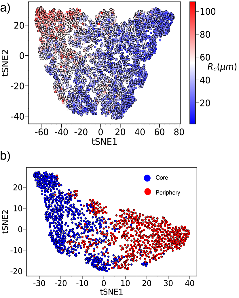
Figure 1: Heterogeneity is radially dependent in an evolving tumor spheroid. (a) Cell trajectories ($\approx 5,000$ ) projected onto tSNE1 and tSNE2. Each dot represents a cell. The cell label depends on the radial distance from the center of the tumor ($R_{c}$). The color gradient is suggestive of extensive dynamical heterogeneity. The blue color represents cells closer to the center whereas cells colored in red are farther away from the center (see the $R_{c}$ scale on the right). (b) Cell trajectories sampled from the core ( blue dots) and periphery ( red dots). There are 1580 (946) core (periphery) cells. Projection of cell trajectories onto t-SNE coordinates shows that the cells in the two regions have resolvable dynamical phase space structure, by which we mean that the data cluster according the motilities of the cells. This is easily seen from the separation of the red and the blue dots.

Results: Figure 1a shows the clustering obtained when the trajectories of cells ($1080\leavevmode\nobreak\ (t_{i},|\delta x_{i}|)$) are projected onto tSNE1 and tSNE2 ($\mathcal{P}=100$). In figure 1, each dot represents a single cell and are colored depending on their distance from the center of the tumor, $R_{c}$. It should be emphasized that in performing t-SNE we did not use the information of the cell distance from the tumor center. The colors aid to visualize the cells. The results in figure 1a show that there is pattern in the way the dots are arranged. Majority of the red dots (cells farthest from tumor core) are at one end, with blue dots at the other end (cells closer to the core). In the other words, there is a dynamic phase separation, which we show below is consequence of cell division and apoptosis. The partitioning into two disjoint patterns in figure 1a implies that the dynamics of the cells is dependent on their distance from the center of tumor as noted in experiments Valencia et al. (2015); Kang et al. (2020). However, the boundary between the two regions (roughly high and low density) is not sharp. The t-SNE method, based on machine learning, is able to delineate massive heterogeneity in a single tumor with identical cells, which is hidden in observables like mean squared displacement or self-intermediate scattering function Malmi-Kakkada et al. (2018); Sinha et al. (2020). Thus, unbiased analyses of the cell trajectories are required to shed light on the origin of DITH in solid tumors Kirkpatrick and Thirumalai (2015); Almendro, Marusyk, and Polyak (2013); Li and Thirumalai (2019).

In a recent experiment Kang et al. (2020), the solid tumor was divided into two core and periphery regions. It was shown that the tumor core (periphery) exhibits sub-diffusive (super-diffusive) dynamics, implying that the cells explore distinct non-overlapping regions of phase space dynamically. In order to assess if t-SNE separates the dynamics in the two regions, we collected position data of core ($R_{c}<30\leavevmode\nobreak\ \mu m$) and periphery ($R_{c}>60\leavevmode\nobreak\ \mu m$). We applied the SNE algorithm on this mixed data set. The figure 1b shows the t-SNE clustering of cells belonging to core (blue dots) and periphery (red dots) ($\mathcal{P}=100$). It is clear from figure 1b that the red and blue cells are approximately phase separated. The distinct dynamical phase space explored by the cells in the core and periphery, as illustrated by figure 1b, sheds light on the non-equilibrium phase separation between tumor core and periphery Kang et al. (2020).

[figure]style=plain,subcapbesideposition=top

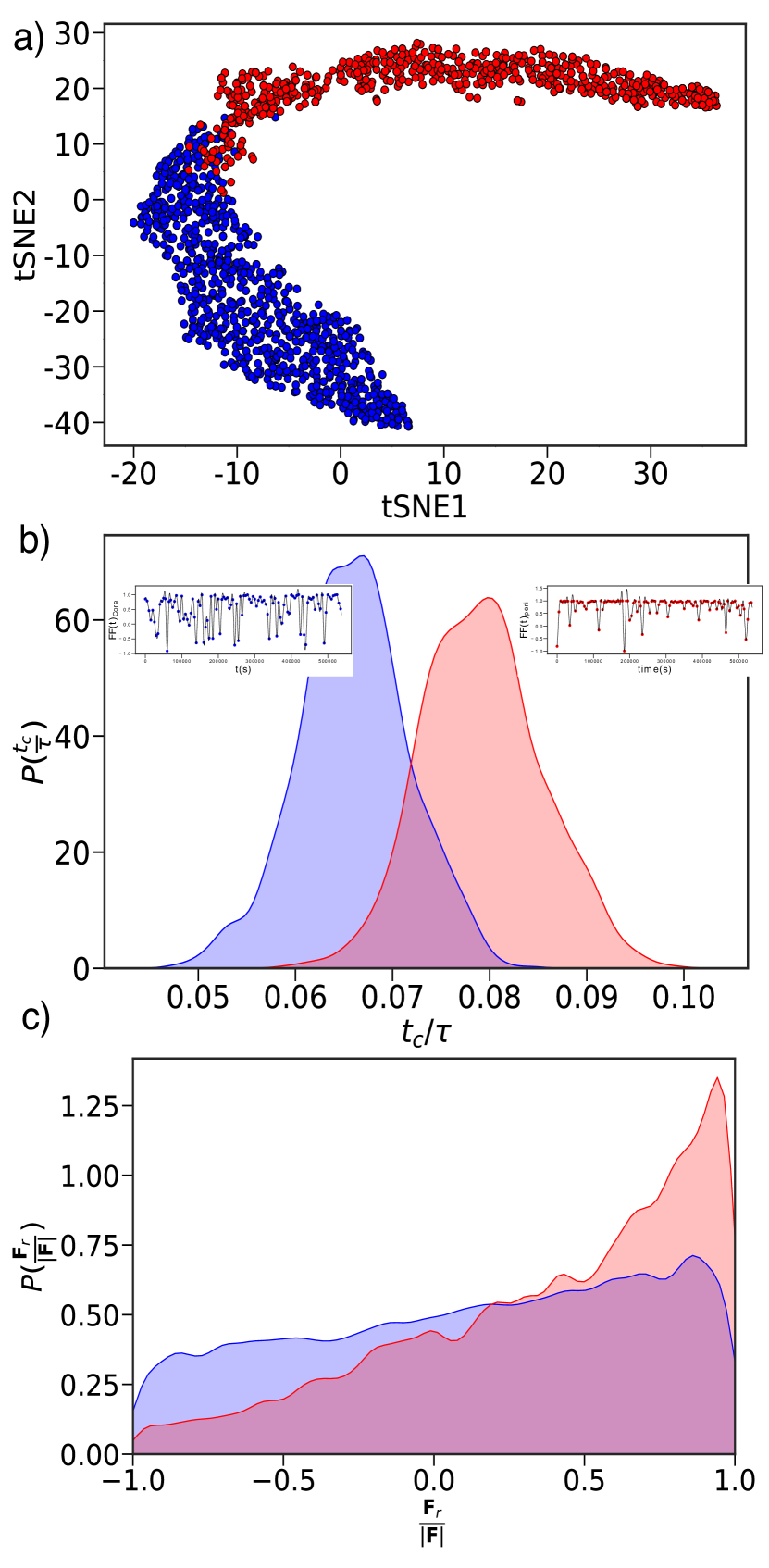
Figure 2: Self generated force due to cell division and apoptosis. (a) t-SNE projection of $FF(t)$ for cells in the core (blue) and periphery (red). The cells in the two regions cluster into distinct regions. (b) Distribution of $\frac{t_{c}}{\tau}$ obtained using Gaussian Process Regression for cells in the core (blue) and periphery (red). Cells in the periphery have higher persistence times (mean value is $\frac{t_{c}}{\tau}=0.08$) compared to cells in the core (average is $\frac{t_{c}}{\tau}=0.06$). Inset on the left (right) shows the FF(t) fit using GPR for cells in core (periphery). The blue (red) dots correspond to cells in the core (periphery) and the solid black line is the GPR fit. (c) Probability distribution of $\frac{{\bf F}_{r}}{|{\bf F}|}$ for cells in the core (blue) and periphery (red). Cells in the periphery experience force predominantly in the radial direction.

Phase separation of cells into core and periphery is a consequence of self-generated active forces (SGAFs) arising from cell division. The SGAF is spatially dependent, leading to distinct cell motility in the core and periphery. In order to understand the dynamical phase space structure of cells predicted by t-SNE, we probed the nature of forces exerted on the cells. We first calculated force-force persistence of the $i^{th}$ cell, $FF_{i}(t)=\frac{{\bf F}_{i}(t+\delta t)\cdot{\bf F}_{i}(t)}{|{\bf F}_{i}(t+\delta t)||{\bf F}_{i}(t)|}$ where ${\bf F}_{i}(t)$ ($|{\bf F}_{i}(t)|$) is the force (force magnitude) on the $i^{th}$ cell at time $t$ and $\delta t=0.05\leavevmode\nobreak\ \tau$ or $40\leavevmode\nobreak\ mins$. $FF_{i}(t)$ is a measure of force persistence an $i^{th}$ cell experiences and takes on values [-1,1]. If $FF(t)=1$ ($FF(t)=-1$), a cell experiences force in the same (opposite) direction at time $t$ and $t+\delta t$. We calculated $FF_{i}(t)$, with $\tau\leq t\leq 11\tau$, for all the cells that belong to core and periphery and performed t-SNE analysis. The t-SNE projection of the $FF(t)$ data in Figure 2a reveals contrasting force persistence for cells in the core and periphery. $FF(t)$ in the two regions partition into two disjoint sets, which is vividly illustrated in Figure 2a. The distinct behavior of force persistence is indicative of the super-diffusive and sub-diffusive behavior of cells in the periphery and core respectively Valencia et al. (2015); Kang et al. (2020). The contrasting force behavior in core and periphery is intrinsically related to spatial propensity for cell division. The increased stress (due to jamming) in the core suppresses cell division whereas cells on the periphery can readily divide Dolega et al. (2017); Alessandri et al. (2013). This imbalance in cell division in the two regions, leads to contrasting force persistence.

We calculated the $\frac{t_{c}}{\tau}$ distribution to quantify how long SGAF is persistent in the two regions. In order to extract $\frac{t_{c}}{\tau}$, we fit $FF_{i}(t)$ using Gaussian process regression (GPR) with the standard RBF kernel ($k(t,t^{\prime})\sim e^{-\frac{(t-t^{\prime})^{2}}{2t_{c}^{2}}}$). Figure 2b shows that the distribution of $\frac{t_{c}}{\tau}$ for cells in the core and periphery are resolvable. Furthermore, we find that the mean persistence time in the periphery ($\frac{t_{c}}{\tau}=0.08$) is greater than in the core ($\frac{t_{c}}{\tau}=0.06$). Increased persistence of forces in the periphery results in greater directed movement. Inset in figure 2b show FF(t) fit using GPR for one cell in core and periphery. Experiments have noted that the cells in the periphery move predominantly radially outward Valencia et al. (2015). Therefore, we calculated the radial force $\frac{{\bf F_{i}}_{r}}{|{\bf F_{i}}|}$ exerted on the cells in the two regions. Here, ${\bf F}_{i,r}={\bf F}_{i}\cdot\hat{{\bf r}_{i}}$, $\hat{{\bf r}_{i}}$ is the radial unit vector, $\hat{{\bf r}_{i}}=\frac{{\bf r}_{i}-{\bf r}_{com}}{|{\bf r}_{i}-{\bf r}_{com}|}$, and ${\bf r}_{com}$ is the center of mass of the tumor. If $\frac{{\bf F_{i}}_{r}}{|{\bf F_{i}}|}=1$, the force is radially directed outward whereas $\frac{{\bf F_{i}}_{r}}{|{\bf F_{i}}|}=-1$ implies inwardly directed force. The probability distribution of $\frac{{\bf F_{i}}_{r}}{|{\bf F_{i}}|}$ for cells in the core is predominantly skewed more towards unity (Figure 2c) than the core cells. The radially outward force explains the invasive characteristics of the cells at the tumor boundary Valencia et al. (2015). These forces originate solely due to the imbalance in cell division in the core and peripheral region of the tumor. Cell division as a source of active stress has been reported before Doostmohammadi et al. (2015), but the emergence of highly persistent nature of forces adds new insights into the physics of tumor expansion.

[figure]style=plain,subcapbesideposition=top

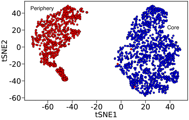
Figure 3: Core and Periphery cells have resolvable interpenetration. Interpenetration, $h_{ij}$ (defined in text), based classification for core and periphery cells using t-SNE. Cells in the core (periphery) are represented using blue (red) dots. The t-SNE algorithm resolves the interpenetration data for cells in the core and periphery.

Armed with the unbiased identification of the cells in the core and the periphery, we set out to find out if these features are manifested in other characteristics as well. Experiments have established that the core cells are tightly packed or jammed Puliafito et al. (2012). Therefore, we expected that the inter-cellular distance can be used to differentiate between the cells in the two regions. We recorded the interpenetration ($h_{ij}$) distances ($h_{ij}$s) for cells in the time window $T_{w1}=\tau_{min}<t<11\tau_{min}$. Figure 3 shows the result of t-SNE clustering based on $h_{ij}$ data for cells in the core and periphery ($\mathcal{P}=50$). To our surprise, the t-SNE algorithm clustered the cells remarkably well with clear phase separation between the cells in the core and the periphery. These results imply that the density in the two regions differ greatly, because the interior cells are jammed whereas the motility of the cells near the periphery is high. The emergence of the radially-dependent density, with jamming in the interior, is consistent with experiments that that show that pressure is higher in the core than at the periphery Dolega et al. (2017).

In order to provide a geometrical interpretation of the SGAF-driven phase separation, we followed Merkel and Manning Merkel and Manning (2018) who predicted that $S=\frac{A}{V^{\frac{2}{3}}}$ could serve as an order parameter for the rigidity transition in 3D confluent tissues. The variables $A$ and $V$ are, respectively, the surface area and volume of the cell. The rigidity transition occurs at $S=5.41$ in three dimensions (see Bi et al. (2016) for results in two dimensions). Because the core (periphery) is solid-like (fluid-like), we expected that the shape parameter would reveal the observed differences in the motilities within a single tumor. We calculated the voronoi volume and area of the cells in at time $\approx 11\tau$. We excluded the cells at the boundary as their voronoi volume is not defined. Figure 4 shows the distributions of the shape parameter distribution in the interior and the periphery. Remarkably, the distribution for cells in the core is narrow with a peak at 5.41, close to the predicted Merkel and Manning (2018) solid to fluid transition value for confluent tissues. However, the packing of cells in the interior in our simulations is qualitatively different, and does not reach confluency. In contrast, the distribution in the boundary are broadly peaked with a mean around 5.6. The inset in figure 4 shows that the cells in boundary have a bigger voronoi volume as compared to cells in the core. We should emphasize the variations in the shape parameter is observed in a tumor in which the low motile and high motile cells are simultaneously present. It appears that the shape parameter is good predictor of the transition from a jammed to a motile (super diffusive) state even in a continuously growing tumor whose dynamics is determined by cell division and apoptosis.

[figure]style=plain,subcapbesideposition=top

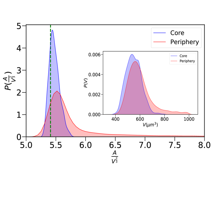
Figure 4: Distribution of the shape parameter in the core and the periphery. Blue curve shows the distribution for the cells in the core and red is for the cells in the periphery. The green line demarcates the solid to fluid boundary at $\frac{A}{V^{\frac{2}{3}}}=5.41$. The inset shows the distributions of the voronoi volume of cells in the core and the periphery.

We used the unsupervised clustering technique (t-SNE)Maaten and Hinton (2008); Van Der Maaten (2014); Van der Maaten and Hinton (2012) to elucidate the extent of heterogeneity in an evolving solid tumor consisting of nearly identical cells. The unbiased t-SNE analysis of the simulation data shows unambiguously that the dynamical behavior of cells in a growing tumor spheroid depends on the distance from the tumor core. The gradual change in the dynamical behavior from a jammed state in the tumor interior to highly motile (super-diffusive) behavior at the periphery is due to the generation of self-generated persistent forces that arises dynamically due to the inequality between cell division and apoptosis rates. The t-SNE method resolves the dynamical phase space structure of identical cells, revealing a plausible mechanism for non-equilibrium phase separation Kang et al. (2020). Our results, establishing dynamic heterogeneity in a single tumor consisting of nearly identical cells, imply that average properties in non-equilibrium systems may have little physical meaning Altschuler and Wu (2010).

We would like to thank Xin Li and Mauro Mugnai for valuable comments on the manuscript. This work was supported by grants from National Science Foundation (PHY 17-08128, PHY-1522550). Additional support was provided by the Collie-Welch Reagents Chair (F-0019).

DATA AVAILABILITY

The data that support the findings of this study are available from the corresponding author upon reasonable request.

References

- Heppner, Miller et al. (1983) G. H. Heppner, B. E. Miller, et al., “Tumor subpopulation interactions in neoplasms,” Biochimica et Biophysica Acta (BBA)-Reviews on Cancer 695, 215–226 (1983).
- McGranahan and Swanton (2015) N. McGranahan and C. Swanton, “Biological and therapeutic impact of intratumor heterogeneity in cancer evolution,” Cancer cell 27, 15–26 (2015).
- Hinohara and Polyak (2019) K. Hinohara and K. Polyak, “Intratumoral heterogeneity: more than just mutations,” Trends in cell biology (2019).
- Gerlinger et al. (2012) M. Gerlinger, A. J. Rowan, S. Horswell, J. Larkin, D. Endesfelder, E. Gronroos, P. Martinez, N. Matthews, A. Stewart, P. Tarpey, et al., “Intratumor heterogeneity and branched evolution revealed by multiregion sequencing,” New England journal of medicine 366, 883–892 (2012).
- Gerlinger et al. (2014) M. Gerlinger, S. Horswell, J. Larkin, A. J. Rowan, M. P. Salm, I. Varela, R. Fisher, N. McGranahan, N. Matthews, C. R. Santos, et al., “Genomic architecture and evolution of clear cell renal cell carcinomas defined by multiregion sequencing,” Nature genetics 46, 225 (2014).
- Harbst et al. (2016) K. Harbst, M. Lauss, H. Cirenajwis, K. Isaksson, F. Rosengren, T. Torngren, A. Kvist, M. C. Johansson, J. Vallon-Christersson, B. Baldetorp, et al., “Multi-region whole-exome sequencing uncovers the genetic evolution and mutational heterogeneity of early-stage metastatic melanoma,” Cancer research , canres–3476 (2016).
- de Bruin et al. (2014) E. C. de Bruin, N. McGranahan, R. Mitter, M. Salm, D. C. Wedge, L. Yates, M. Jamal-Hanjani, S. Shafi, N. Murugaesu, A. J. Rowan, et al., “Spatial and temporal diversity in genomic instability processes defines lung cancer evolution,” Science 346, 251–256 (2014).
- Zhang et al. (2014) J. Zhang, J. Fujimoto, J. Zhang, D. C. Wedge, X. Song, J. Zhang, S. Seth, C.-W. Chow, Y. Cao, C. Gumbs, et al., “Intratumor heterogeneity in localized lung adenocarcinomas delineated by multiregion sequencing,” Science 346, 256–259 (2014).
- Cao et al. (2015) W. Cao, W. Wu, M. Yan, F. Tian, C. Ma, Q. Zhang, X. Li, P. Han, Z. Liu, J. Gu, et al., “Multiple region whole-exome sequencing reveals dramatically evolving intratumor genomic heterogeneity in esophageal squamous cell carcinoma,” Oncogenesis 4, e175 (2015).
- Richards et al. (2018) R. Richards, D. Mason, R. Levy, R. Bearon, and V. See, “4d imaging and analysis of multicellular tumour spheroid cell migration and invasion,” bioRxiv , 443648 (2018).
- Valencia et al. (2015) A. M. J. Valencia, P.-H. Wu, O. N. Yogurtcu, P. Rao, J. DiGiacomo, I. Godet, L. He, M.-H. Lee, D. Gilkes, S. X. Sun, et al., “Collective cancer cell invasion induced by coordinated contractile stresses,” Oncotarget 6, 43438 (2015).
- Kang et al. (2020) W. Kang, J. Ferruzzi, C.-P. Spatarelu, Y. L. Han, Y. Sharma, S. Koehler, J. P. Butler, D. Roblyer, M. H. Zaman, M. Guo, et al., “Tumor invasion as non-equilibrium phase separation,” bioRxiv (2020).
- Han et al. (2019) Y. L. Han, A. F. Pegoraro, H. Li, K. Li, Y. Yuan, G. Xu, Z. Gu, J. Sun, Y. Hao, S. K. Gupta, et al., “Cell swelling, softening and invasion in a three-dimensional breast cancer model,” Nature Physics , 1–8 (2019).
- Palamidessi et al. (2019) A. Palamidessi, C. Malinverno, E. Frittoli, S. Corallino, E. Barbieri, S. Sigismund, G. V. Beznoussenko, E. Martini, M. Garre, I. Ferrara, C. Tripodo, F. Ascione, E. A. Cavalcanti-Adam, Q. Li, P. P. Di Fiore, D. Parazzoli, F. Giavazzi, R. Cerbino, and G. Scita, “Unjamming overcomes kinetic and proliferation arrest in terminally differentiated cells and promotes collective motility of carcinoma,” Nature Materials 18, 1252–1263 (2019).
- Sinha et al. (2020) S. Sinha, A. N. Malmi-Kakkada, X. Li, H. S. Samanta, and D. Thirumalai, “Spatially heterogeneous dynamics of cells in a growing tumor spheroid: Comparison between theory and experiments,” Soft Matter 16, 5294–5304 (2020).
- Kirkpatrick and Thirumalai (2015) T. Kirkpatrick and D. Thirumalai, “Colloquium: Random first order transition theory concepts in biology and physics,” Reviews of Modern Physics 87, 183 (2015).
- Berthier and Barrat (2002) L. Berthier and J.-L. Barrat, “Nonequilibrium dynamics and fluctuation-dissipation relation in a sheared fluid,” The Journal of Chemical Physics 116, 6228–6242 (2002).
- Malmi-Kakkada et al. (2018) A. N. Malmi-Kakkada, X. Li, H. S. Samanta, S. Sinha, and D. Thirumalai, “Cell growth rate dictates the onset of glass to fluidlike transition and long time superdiffusion in an evolving cell colony,” Physical Review X 8, 021025 (2018).
- Maaten and Hinton (2008) L. v. d. Maaten and G. Hinton, “Visualizing data using t-sne,” Journal of machine learning research 9, 2579–2605 (2008).
- Van Der Maaten (2009) L. Van Der Maaten, “Learning a parametric embedding by preserving local structure,” in Artificial Intelligence and Statistics (2009) pp. 384–391.
- Van der Maaten and Hinton (2012) L. Van der Maaten and G. Hinton, “Visualizing non-metric similarities in multiple maps,” Machine learning 87, 33–55 (2012).
- Van Der Maaten (2014) L. Van Der Maaten, “Accelerating t-sne using tree-based algorithms,” The Journal of Machine Learning Research 15, 3221–3245 (2014).
- Kobak and Berens (2019) D. Kobak and P. Berens, “The art of using t-sne for single-cell transcriptomics,” Nature communications 10, 1–14 (2019).
- Linderman et al. (2019) G. C. Linderman, M. Rachh, J. G. Hoskins, S. Steinerberger, and Y. Kluger, “Fast interpolation-based t-sne for improved visualization of single-cell rna-seq data,” Nature methods 16, 243–245 (2019).
- Dimitriadis, Neto, and Kampff (2018) G. Dimitriadis, J. P. Neto, and A. R. Kampff, “T-sne visualization of large-scale neural recordings,” Neural computation 30, 1750–1774 (2018).
- Carrasquilla and Melko (2017) J. Carrasquilla and R. G. Melko, “Machine learning phases of matter,” Nature Physics 13, 431–434 (2017).
- Ch’ng, Vazquez, and Khatami (2018) K. Ch’ng, N. Vazquez, and E. Khatami, “Unsupervised machine learning account of magnetic transitions in the hubbard model,” Physical Review E 97, 013306 (2018).
- Day et al. (2019) A. G. Day, M. Bukov, P. Weinberg, P. Mehta, and D. Sels, “Glassy phase of optimal quantum control,” Physical review letters 122, 020601 (2019).
- Malmi-Kakkada et al. (2019) A. Malmi-Kakkada, X. Li, S. Sinha, and D. Thirumalai, “Dual role of cell-cell adhesion in tumor suppression and proliferation,” arXiv preprint arXiv:1906.11292 (2019).
- Samanta, Sinha, and Thirumalai (2020) H. S. Samanta, S. Sinha, and D. Thirumalai, “Far from equilibrium dynamics of tracer particles embedded in a growing multicellular spheroid,” arXiv preprint arXiv:2003.12941 (2020).
- Wattenberg, Viégas, and Johnson (2016) M. Wattenberg, F. Viégas, and I. Johnson, “How to use t-sne effectively,” Distill 1, e2 (2016).
- Almendro, Marusyk, and Polyak (2013) V. Almendro, A. Marusyk, and K. Polyak, “Cellular Heterogeneity and Molecular Evolution in Cancer,” Ann. Rev. Pathol. Med. Dis. 8, 277–302 (2013).
- Li and Thirumalai (2019) X. Li and D. Thirumalai, “Share, but unequally: a plausible mechanism for emergence and maintenance of intratumour heterogeneity,” Journal of the Royal Society Interface 16, 20180820 (2019).
- Dolega et al. (2017) M. E. Dolega, M. Delarue, F. Ingremeau, J. Prost, A. Delon, and G. Cappello, “Cell-like pressure sensors reveal increase of mechanical stress towards the core of multicellular spheroids under compression,” Nature Communications 8, 14056 (2017).
- Alessandri et al. (2013) K. Alessandri, B. R. Sarangi, V. V. Gurchenkov, B. Sinha, T. R. Kießling, L. Fetler, F. Rico, S. Scheuring, C. Lamaze, A. Simon, et al., “Cellular capsules as a tool for multicellular spheroid production and for investigating the mechanics of tumor progression in vitro,” Proceedings of the National Academy of Sciences 110, 14843–14848 (2013).
- Doostmohammadi et al. (2015) A. Doostmohammadi, S. P. Thampi, T. B. Saw, C. T. Lim, B. Ladoux, and J. M. Yeomans, “Celebrating soft matter’s 10th anniversary: cell division: a source of active stress in cellular monolayers,” Soft Matter 11, 7328–7336 (2015).
- Puliafito et al. (2012) A. Puliafito, L. Hufnagel, P. Neveu, S. Streichan, A. Sigal, D. K. Fygenson, and B. I. Shraiman, “Collective and single cell behavior in epithelial contact inhibition,” Proceedings of the National Academy of Sciences 109, 739–744 (2012).
- Merkel and Manning (2018) M. Merkel and M. L. Manning, “A geometrically controlled rigidity transition in a model for confluent 3d tissues,” New Journal of Physics 20, 022002 (2018).
- Bi et al. (2016) D. Bi, X. Yang, M. C. Marchetti, and M. L. Manning, “Motility-driven glass and jamming transitions in biological tissues,” Physical Review X 6, 021011 (2016).
- Altschuler and Wu (2010) S. J. Altschuler and L. F. Wu, “Cellular heterogeneity: do differences make a difference?” Cell 141, 559–563 (2010).