Terahertz field induced near-cutoff even-order harmonics in femtosecond laser

Abstract

High-order harmonic generation by femtosecond laser pulse in the presence of a moderately strong terahertz (THz) field is studied under the strong field approximation, showing a simple proportionality of near-cutoff even-order harmonic (NCEH) amplitude to the THz electric field. The formation of the THz induced-NCEHs is analytically shown for both continuous wave and Gaussian pulse. The perturbation analysis with regard to the frequency ratio of the THz field to the femtosecond pulse shows the THz-induced NCEHs originates from its first-order correction, and the available parametric conditions for the phenomenon is also clarified. As the complete characterization of the time-domain waveform of broadband THz field is essential for a wide variety of applications, the work provides an alternative time-resolved field-detection technique, allowing for a robust broadband characterization of pulses in THz spectral range.

I Introduction

The development of terahertz (THz) technology has motivated a broad range of scientific studies and applications in material science, chemistry and biology. The THz light is especially featured by the availability to access low-energy excitations, providing a fine tool to probe and control quasi-particles and collective excitations in solids, to drive phase transitions and associated changes in material properties, and to study rotations and vibrations in molecular systems Salén et al. (2019).

In THz science, the capabilities of ultra-broadband detection are essential to the diagnostics of THz field of a wide spectral range. The most common detection schemes are based on the photoconductive switches (PCSs) Jepsen et al. (1996); van Exter and Grischkowsky (1990) or the electro-optic sampling (EOS) Wu and Zhang (1995). Especially the EOS technique, which uses part of the laser pulse generating the THz field to sample the latter, has been widely applied in the THz time-domain spectroscopy, pump-probe experiments and dynamic matter manipulation Lee (2009). Nevertheless, both PCSs and EOS require particular mediums — photoconductive antenna for the former and electro-optic crystal for the latter. Due to inherent limitations of the detection media, including dispersion, absorption, long carrier lifetime, and lattice resonances Ferguson and Zhang (2002), the typical accessible bandwidth of detected THz is limited below 7 THz Shen et al. (2003); Somma et al. (2015); Kübler et al. (2005); Wu and Zhang (1997); Zhang et al. (2016).

On the other hand, gas-based schemes, including air-breakdown coherent detection Dai et al. (2006), air-biased coherent detection (ABCD) Karpowicz et al. (2008), optically biased coherent detection Li et al. (2015), THz radiation enhanced emission of fluorescence Liu et al. (2010) et al., allow for ultra-broadband detections since gases being continuously renewable show no appreciable dispersion or phonon absorption Lu and Zhang (2014), thus effectively extending the accessible spectral range beyond 10 THz. In particular, the ABCD utilizes the THz-field-induced second harmonics (TFISH) Cook et al. (1999) to sense the THz transient through a third-order nonlinear process. The THz field mixed with a bias electric field breaks the symmetry of air and induces the frequency doubling of the propagating probe beam. Such a nonlinear mixing results in a signal of the intensity proportional to the THz electric field, allowing for the coherent detection by which both amplitude and phase of the THz transient can be reconstructed.

The air-based broadband THz detection utilizing the laser induced air plasma as the sensor medium is essentially an inverse process of THz wave generation (TWG) in femtosecond laser gas breakdown plasma. Both involve rather complicated processes dominated by the strong field photoionization. From the perspective of single-atom based strong field theory, the TWG has been interpreted as the near-zero-frequency radiation due to the continuum-continuum transition of photoelectron Zhou et al. ; Zhang et al. (2020a, b), complementary to the widely acknowledged mechanism for high-order harmonic generation (HHG) — the continuum-bound transition that emits high energy photons when the released electron after the ionization recollides with the parent ion Lewenstein et al. (1994).

Under the same nonperturbative theoretical framework depicting the strong-field induced radiation, the TWG and the HHG within one atom, however, present different facets of dynamics of electron wave packet, providing potential strategies to either characterize the system or to profile external light fields. For example, the synchronized measurements on angle-resolved TWG and HHG from aligned molecules allow for reliable descriptions of molecular structures Huang et al. (2015). On the other hand, the presence of THz or static fields may drastically affect the photoionization dynamics and reshape electron trajectories, eventually altering photoelectron spectra and HHG radiations. Applying the widely used streaking technique, the influence on photoelectron spectra from an additional THz transient can help characterize the time structure of an attosecond pulse train, e.g., pulse duration of individual harmonic Ardana-Lamas et al. (2016). The altered HHG spectral features by THz or static fields include the increased odd-order harmonic intensity in the low end of the plateau, the significant production of even-order harmonics Bao and Starace , the double-plateau structure Wang et al. (1998) and high-frequency extension Taranukhin and Shubin (2000); Hong et al. (2009). The substantially extended HHG cutoff in combined fields creates ultrabroad supercontinuum spectrum, allowing for the generation of single attosecond pulses. For example, the combination of a chirped laser and static electric field has been proposed to obtain isolated pulse as short as 10 attoseconds Xiang et al. (2009).

In this work, we study the influence of an additional moderately strong THz field on the HHG by femtosecond laser pulse. By "moderately" we mean the THz field is easily attainable in nowadays laboratories — its intensity is not as high as to modify global harmonic features as considered in previous theoretical works. Instead, we focus on the more subtle THz-induced even-order harmonics. The dependence of all-order HHG on time delay between the THz field and the femtosecond pulse is studied, showing the near-cutoff even-order harmonics (NCEHs) are of particular synchronicity with the external THz field. Accordingly, the measurement of THz induced NCEHs, similar to the widely used TFISH, is supposed to provide an alternative all-optical ultrabroad bandwidth method to characterize the time-domain THz transient. The influence of the THz field on NCEHs is theoretically investigated under the strong field approximation, showing a direct link inbetween, further confirming the availability of the detection scheme.

The paper is organized as follows: In Sec. II, we present time-delay dependent all-order HHG calculations and show the significant correlation between NCEHs and the external THz field, illustrating the possible schematics to reconstruct the time-domain THz field using NCEHs. In Sec. III, the detailed analysis of the NCEHs is presented. A brief retrospect of the analytical derivation for odd-order harmonics is given in Sec. III.1, followed by the discussion in Sec. III.2 on the simplest case, the NCEHs in fields of continuous wave. When a femtosecond laser has a finite pulse width, the influence from pulse envelope is shown in Sec. III.3, where the action for a Gaussian envelope is explicitly derived. In Sec. III.4, a complete description of the THz-induced NCEHs in femtosecond pulse is presented, showing the relation between the NCEH and the THz field at the center of the femtosecond laser pulse. In the end, exemplary reconstruction schematics are shown with parametric conditions discussed for the applicability.

II Scheme of Coherent Detection and Numerical Simulations

We consider an atom subject to combined fields including a linearly polarized femtosecond laser pulse $E_{0}(t)$ and a THz field $E_{1}(t)$. With both polarizations along the same direction, the total fields read $E(t)=E_{0}(t)+E_{1}(t)$. Denoting the associated vector potentials by $A(t)=A_{0}(t)+A_{1}(t)$, we evaluate the harmonics using the Lewenstein model Lewenstein et al. (1994) under the strong field approximation Keldysh (1965); Faisal (1973); Reiss (1980), which is usually applicable in the tunneling regimes, providing a reasonable and intuitive description of harmonic radiation from highly energetic recolliding electrons. The time-dependent dipole moment $d(t)$ in Ref. Lewenstein et al. (1994) as an integration over the intermediate momentum can be dramatically simplified by applying the stationary phase approximation, yielding

$$d(t) = \text{i}\int_{0}^{\infty}\mathrm{d}\tau\left(\frac{\pi}{\epsilon+\text{i}\tau/2}\right)^{3/2}\mu^{\ast}[p_{\operatorname{st}}(t,\tau)+A(t)]$$ (1)

$$\times\mu[p_{\operatorname{st}}(t,\tau)+A(t-\tau)]E(t-\tau)\mathrm{e}^{-\text{i}S(t,\tau)}+\text{c.c.},$$

where integration variable $\tau$ is the return time of the electron, i.e., the interval between the instants of ionization and rescattering. In this work, atomic units are used unless noted otherwise. The dipole matrix element $\mu(k)=\langle k|\hat{x}|\Psi_{0}\rangle$ between bound state $|\Psi_{0}\rangle$ and continuum state $|k\rangle$ of momentum $k$ is given by $\mathrm{i}\partial_{k}\langle k|\Psi_{0}\rangle$ along the polarization direction. Taking $|\Psi_{0}\rangle$ the $1s$ state of a hydrogen-like atom for example, $\mu(k)=-\text{i}2^{7/2}(2I_{p})^{5/4}k/[\pi(k^{2}+2I_{p})^{3}]$, where $I_{p}$ is the ionization potential. In Eq. (1), the action reads

$$S(t,\tau) = \int_{t-\tau}^{t}\mathrm{d}t^{\prime}\left(\frac{1}{2}[p_{\operatorname{st}}(t,\tau)-A(t^{\prime})]^{2}+I_{p}\right),$$ (2)

and the stationary momentum $p_{\operatorname{st}}(t,\tau)=-[\alpha(t)-\alpha(t-\tau)]/\tau$ is determined by the electron excursion $\alpha(t)=\int^{t}\mathrm{d}t^{\prime}A(t^{\prime})$ after the electron is released by external light fields. The subsequent spread of the continuum electron wave packet is depicted by $\left[\pi/\left(\epsilon+\text{i}\tau/2\right)\right]^{3/2}$ in the integral of Eq. (1) with an infinitesimal $\epsilon$.

Evaluating $d(t)$ of Eq. (1) and $|\tilde{d}(\omega)|$ from its Fourier transform, we demonstrate in Fig. 1 the all-order harmonics as a function of the time delay between a near-infrared pulse and a THz field. The near-infrared pulse has the vector potential of a Gaussian envelope, $A_{0}(t)=(E_{0}/\omega_{0})\mathrm{e}^{-t^{2}/(2\sigma^{2})}\sin(\omega_{0}t)$, with $\omega_{0}=0.0353$ (1.3 $\mu$m), $E_{0}=0.06$ (intensity $I=1.3\times 10^{14}$ W/cm²), $\sigma=2106$ (FWHM of 120 fs). The THz field is modeled by $A_{1}(t)\propto-(E_{1}/\omega_{1})(\omega_{1}t)^{-10}/[\exp(a/\omega_{1}t)-1]\sin(\omega_{1}t+\phi)$ with $a=50$, $E_{1}=2\times 10^{-5}$ (100 kV/cm), $\omega_{1}=2\times 10^{-4}$ (1 THz) and $\phi=0.3\pi$, and the corresponding electric field $E_{1}(t)=-\partial_{t}A_{1}(t)$ is shown in Fig. 1(a).

Figure 1: Schematics of the reconstruction of THz field with near-cutoff even-order harmonics, which uses a femtosecond laser pulse to scan over a THz field and to record the generated harmonics as a function of the time delay between the fields. Panel (a) shows an exemplary THz field with $\omega_{1}=2\times 10^{-4}$ (1 THz), and $E_{1}=2\times 10^{-5}$ (100 kV/cm). Without the THz field, panel (b) shows the harmonics generated by a femtosecond pulse with  $\omega_{0}=0.0353$ (1.3 $\mu$m), $E_{0}=0.06$ ($I=1.3\times 10^{14}$ W/cm²) and $\sigma=2106$ (FWHM of 120 fs). With the THz field, panel (c) shows the all-order harmonics versus the time delay. The difference $\Delta|\tilde{d}(\omega)|$ between the harmonics with THz field, as given in (c), and the one without THz field, as shown in (b), is presented in panel (d) in the linear scale. All near-cutoff even-order harmonics, as indicated by the box around $E_{\text{cutoff}}=I_{p}+3.17U_{p}$, exhibits synchronous change with the intensity of the THz field.

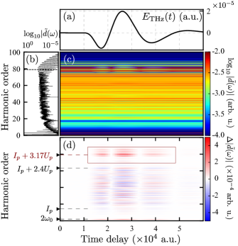
When the THz field is absent, Fig. 1(b) shows $|\tilde{d}(\omega)|$ in the logarithmic scale with a typical plateau structure between the 20th- and 80th-order. The harmonic yield dramatically decreases beyond the cutoff around 80th-order, as depicted by the maximum kinetic energy of a recolliding electron, $E_{\text{cutoff}}=I_{p}+3.17U_{p}$, where $U_{p}=E_{0}^{2}/4\omega_{0}^{2}$ is the ponderomotive energy of the electron.

When the THz field is present, the full scope of all-order $|\tilde{d}(\omega)|$ in the logarithmic scale versus the time delay is presented in Fig. 1(c). To better observe the influence from the accompanied THz field, the difference between $|\tilde{d}(\omega)|$ with and without THz field, $\Delta|\tilde{d}(\omega)|$, is shown in Fig. 1(d) in the linear scale, with positive and negative values indicated by distinct colors. A close scrutiny reveals most of the nonvanishing $\Delta|\tilde{d}(\omega)|$ shown in (d) appear at even orders. In the low-order region, the second-order harmonic follows the change of THz intensity similar to the phenomenon utilized by TFISH, though the applicability of the model in this low-order region is dubious. As the harmonic order increases, the delay dependence of harmonics loses the regularity and the distribution seems rather chaotic. When the harmonic order increases up to the near-cutoff region, the delay-dependent harmonic yields, however, again follow the time profile of $|E_{1}(t)|$. Such a concurrence is noteworthy, since it provides an alternative detection strategy to characterize an arbitrary time-domain THz waveform.

III Analysis of near-cutoff even-order harmonics

III.1 Monochromatic light field

Before the analysis of THz induced modulation on NCEHs, we retrospect the simplest case where the HHG is induced by a monochromatic field of continuous wave $E(t)=E_{0}\cos(\omega_{0}t)$ and the vector potential $A(t)=A_{0}\sin(\omega_{0}t)$ with $E_{0}=-A_{0}\omega_{0}$ Lewenstein et al. (1994). For concision, defining phases $\varphi_{t}=\omega_{0}t$ and $\varphi_{\tau}=\omega_{0}\tau$, we have $p_{\operatorname{st}}(\varphi_{t},\varphi_{\tau})=A_{0}[\cos\varphi_{t}-\cos(\varphi_{t}-\varphi_{\tau})]/\varphi_{\tau}$, and the action in Eq. (2) reads

$$S_{0}(\varphi_{t},\varphi_{\tau}) = F_{0}(\varphi_{\tau})-\left(\frac{U_{p}}{\omega_{0}}\right)C_{0}(\varphi_{\tau})\cos(2\varphi_{t}-\varphi_{\tau})$$ (3)

with the ponderomotive potential $U_{p}=E_{0}^{2}/4\omega_{0}^{2}=A_{0}^{2}/4$, $F_{0}(\varphi_{\tau})=[(I_{p}+U_{p})/\omega_{0}]\varphi_{\tau}-(2U_{p}/\omega_{0})(1-\cos\varphi_{\tau})/\varphi_{\tau}$, and

$$C_{0}(\varphi_{\tau}) = \sin\varphi_{\tau}-\frac{4\sin^{2}(\varphi_{\tau}/2)}{\varphi_{\tau}}.$$ (4)

Here, subscript "0" in $S_{0}$ is used to label the action without the influence from the additional accompanied field, i.e., the THz field as will be discussed in the subsequent sections. Applying the Anger-Jacobi expansion, the exponential part $\exp(-\mathrm{i}S_{0})$ with $S_{0}$ of Eq. (3) reads $\exp[-\mathrm{i}S_{0}(\varphi_{t},\varphi_{\tau})]=\exp[-\mathrm{i}F_{0}(\varphi_{\tau})]\sum_{M=-\infty}^{\infty}\mathrm{i}^{M}J_{M}(U_{p}C_{0}(\varphi_{\tau})/\omega_{0})\exp[\mathrm{i}M(\varphi_{\tau}-2\varphi_{t})]$.

In Eq. (1), the part including dipole matrix elements $\mu^{\ast}[p_{\operatorname{st}}(\varphi_{t},\varphi_{\tau})+A(\varphi_{t})]\mu[p_{\operatorname{st}}(\varphi_{t},\varphi_{\tau})+A(\varphi_{t}-\varphi_{\tau})]E(\varphi_{t}-\varphi_{\tau})$ can be represented by Fourier series $\sum_{n}b_{n}(\varphi_{\tau})\exp\left[-\text{i}(2n+1)\varphi_{t}\right]$ with respect to $\varphi_{t}$. For simplicity, we assume the dipole moment of the form $\mu(p)\sim\mathrm{i}p$, leading to mostly vanishing $b_{n}$ except for ones with $2n+1=\pm 1$ and $\pm 3$.

Applying the above expansions and substituting $n=K-M$,  Eq. (1) eventually has the form

$$d_{0}(t) = \sum_{K=-\infty}^{\infty}\tilde{d}_{0,2K+1}\mathrm{e}^{-\mathrm{i}(2K+1)\varphi_{t}}.$$ (5)

For $K\geqslant 0$, the coefficients for odd-order harmonics are given by

$$\tilde{d}_{0,2K+1} = \mathrm{i}\int_{0}^{\infty}\mathrm{d}\tau\left(\frac{\pi}{\epsilon+\text{i}\tau/2}\right)^{3/2}\mathrm{e}^{-\mathrm{i}F_{0}(\varphi_{\tau})}$$ (6)

$$\times\sum_{M=0}^{\infty}\mathrm{i}^{M}\mathrm{e}^{\mathrm{i}M\varphi_{\tau}}J_{M}\left(\frac{U_{p}}{\omega_{0}}C_{0}(\varphi_{\tau})\right)b_{K-M}(\varphi_{\tau})$$

$$+\text{c.c.}$$

while coefficients of all even-order harmonics vanish due to the restricted value range of $n$ as long as the atomic potential is spherically symmetric.

III.2 THz field induced NCEHs

An extra THz field of the same polarization direction, $A_{1}(t)$, induces even-order harmonics. In the followings, the detailed analysis of NCEHs is presented to show their relations with the THz field. Defining $p_{\text{st},i}$ the stationary momentum for a single field $i$ of vector potential $A_{i}(t)$ with $i=0$ and 1, the stationary momentum when both fields are present satisfies $p_{\text{st}}=p_{\text{st},0}+p_{\text{st},1}$. Also, let $S_{i}(t,\tau)=\frac{1}{2}\int_{t-\tau}^{t}\left[p_{\text{st},i}+A_{i}(t)\right]^{2}+I_{p}\tau$ be the single action for the $i$th field and note that $\int_{t-\tau}^{t}A_{i}(t^{\prime})\mathrm{d}t^{\prime}=p_{\text{st},i}\tau$, the total action $S(t,\tau)$ relates to partial action $S_{i}(t,\tau)$ by

$$S(t,\tau) = S_{0}(t,\tau)+[S_{1}(t,\tau)-I_{p}\tau]$$ (7)

$$-p_{\text{st},0}p_{\text{st},1}\tau+\int_{t-\tau}^{t}A_{0}(t^{\prime})A_{1}(t^{\prime})\mathrm{d}t^{\prime}.$$

Given the vector potential of the additional THz field $A_{1}(t)=A_{1}\cos(\omega_{1}t+\phi)$ with $\omega_{1}\ll\omega_{0}$ and $\phi$ an arbitrary initial phase, we define the frequency ratio $\varepsilon=\omega_{1}/\omega_{0}\ll 1$. Substituting $A_{0}(t)$ and $A_{1}(t)$ into Eq. (7), it is shown that the first-order correction with regard to $\varepsilon$ arises completely from the cross term in Eq. (7) (i.e., the two terms on the second line), while $S_{1}(t,\tau)-I_{p}\tau$ merely has the contribution of $\mathcal{O}(\varepsilon^{2})$. Retaining terms of $S(t,\tau)$ only up to the first order of $\varepsilon$, we have the yielding action $S(\varphi_{t},\varphi_{\tau})\simeq S_{0}(\varphi_{t},\varphi_{\tau})+\Delta S(\varphi_{t},\varphi_{\tau})$ with the THz-induced correction

$$\Delta S(\varphi_{t},\varphi_{\tau}) = -p_{\text{st},0}p_{\text{st},1}\tau+\int_{t-\tau}^{t}A_{0}(t^{\prime})A_{1}(t^{\prime})\mathrm{d}t^{\prime}$$ (8)

$$\simeq \varepsilon\frac{A_{0}A_{1}}{\omega_{0}}\sin\phi C_{1}(\varphi_{\tau})\cos\left(\varphi_{t}-\frac{\varphi_{\tau}}{2}\right)$$

and $C_{1}(\varphi_{\tau})=\varphi_{\tau}\cos(\varphi_{\tau}/2)-2\sin(\varphi_{\tau}/2)$.

The action correction $\Delta S(\varphi_{t},\varphi_{\tau})$ can also be treated with Anger-Jacobi expansion, $\exp[-\mathrm{i}\Delta S(\varphi_{t},\varphi_{\tau})]=\sum_{N=-\infty}^{\infty}\mathrm{i}^{N}J_{N}(-\varepsilon A_{0}A_{1}\sin\phi C_{1}(\varphi_{\tau})/\omega_{0})\exp[\mathrm{i}N(\varphi_{\tau}/2-\varphi_{t})]$, resulting in the expansion for the full action,

$$\mathrm{e}^{-\mathrm{i}S(\varphi_{t},\varphi_{\tau})} = \mathrm{e}^{-\mathrm{i}F_{0}(\varphi_{\tau})}\sum_{M,N=-\infty}^{\infty}\mathrm{i}^{M+N}J_{M}\left(\frac{U_{p}}{\omega_{0}}C_{0}(\varphi_{\tau})\right)$$ (9)

$$\times J_{N}\left(-\varepsilon\frac{A_{0}A_{1}}{\omega_{0}}\sin\phi C_{1}(\varphi_{\tau})\right)$$

$$\times\mathrm{e}^{\mathrm{i}\left(M+\frac{N}{2}\right)\varphi_{\tau}}\mathrm{e}^{-\mathrm{i}(2M+N)\varphi_{t}}.$$

Considering that the relatively small THz electric component $E_{1}(t)$ is negligible, the similar Fourier series expansion,  $\mu^{\ast}[p_{\operatorname{st}}(\varphi_{t},\varphi_{\tau})+A(\varphi_{t})]\mu[p_{\operatorname{st}}(\varphi_{t},\varphi_{\tau})+A(\varphi_{t}-\varphi_{\tau})]E(\varphi_{t}-\varphi_{\tau})=\sum_{M}b_{M}(\varphi_{\tau})\exp\left[-\text{i}(2M+1)\varphi_{t}\right]$, can still be performed as in Sec. III.1 with $E(\varphi_{t}-\varphi_{\tau})\simeq E_{0}(\varphi_{t}-\varphi_{\tau})$.

Figure 2: The function $2|C_{0}(\varphi_{\tau})|$ (solid line) and $|C_{1}(\varphi_{\tau})|$ (dashed line) versus $\varphi_{\tau}$ of the return time. The maximum of the $2|C_{0}(\varphi_{\tau})|$ is associated to the maximum kinetic energy gain that corresponds to the cutoff energy of the HHG, as indicated by the black line for $3.17U_{p}$. The shaded area (light blue) highlights $\varphi_{\tau}$ contributing to the near-cutoff harmonic spectrum of the the energy between $2.4U_{p}$ (red line) and $3.17U_{p}$ (black line).

Substituting the above expansion and Eq. (9) into Eq. (1), we obtain

$$d(t) = \text{i}\sum_{n=-\infty}^{\infty}\int_{0}^{\infty}\mathrm{d}\tau\left(\frac{\pi}{\epsilon+\text{i}\tau/2}\right)^{3/2}b_{n}(\varphi_{\tau})\mathrm{e}^{-\mathrm{i}F_{0}(\varphi_{\tau})}$$ (10)

$$\times\sum_{M,N=-\infty}^{\infty}\mathrm{i}^{M+N}J_{M}\left(\frac{U_{p}}{\omega_{0}}C_{0}(\varphi_{\tau})\right)$$

$$\times J_{N}\left(-\varepsilon\frac{A_{0}A_{1}}{\omega_{0}}\sin\phi C_{1}(\varphi_{\tau})\right)$$

$$\times\mathrm{e}^{\mathrm{i}\left(M+\frac{N}{2}\right)\varphi_{\tau}}\mathrm{e}^{-\mathrm{i}[2(M+n)+N+1]\varphi_{t}}+\text{c.c.}.$$

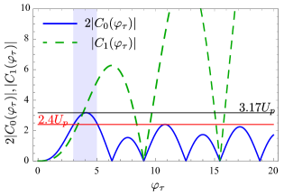
The near-cutoff harmonics are usually featured with restricted range of $\varphi_{\tau}$. As shown in Fig. 2, the photon energy within the range $2.4U_{p}<2|C_{0}(\varphi_{\tau})|<3.17U_{p}$ requires $\varphi_{\tau}\in[3,5]$, corresponding to the first return of the released electron (see also Fig. 1 of Ref. Lewenstein et al. (1994)). Within the range of $\varphi_{\tau}$ contributing to the near-cutoff harmonics, as indicated by the shaded area in Fig. 2, the globally increasing function $C_{1}(\varphi_{\tau})$ also remains low, resulting in the whole argument of $J_{N}$ being small. Taking a typical 800 nm, $1\times 10^{14}$ W/cm² femtosecond pulse and 1 THz, 1 MV/cm THz field for example, the argument in $J_{N}(z)$ is roughly $|z|\approx 0.3$. Since $J_{N}(z)$ becomes exponentially small when $N>|z|$, only when $N=0,\pm 1$ does $J_{N}(z)$ significantly contribute, since we have the typical value $|z|<1$. Using $J_{N}(z)\simeq(z/2)^{N}/\Gamma(N+1)$ when $z\rightarrow 0$ Abramowitz and Stegun (1965), we find from Eq. (10) that $d(t)=d_{0}(t)+d_{1}(t)+\mathcal{O}(\varepsilon^{2})$, where $d_{0}(t)$, simply given by Eq. (5) for odd-order harmonics in a monochromatic field, stems from the contribution of $N=0$ as $J_{0}(z)=1$. The odd-order harmonics are barely influenced by the additional low-frequency field around the near-cutoff region as long as the THz field remains relatively low to fulfill $|z|<1$ for $J_{N}(z)$. It is noteworthy that an extra correction to the dipole moment, $d_{1}(t)$, is induced by the THz field, corresponding to $N=\pm 1$ as $J_{\pm 1}(z)=\pm z/2$. In contrast to Eq. (5), we have $d_{1}(t)$ in the frequency domain,

$$d_{1}(t) = \sum_{K=-\infty}^{\infty}\tilde{d}_{1,2K}\mathrm{e}^{-\mathrm{i}(2K)\varphi_{t}},$$

containing only even-order harmonics, whose coefficients are given by

$$\tilde{d}_{1,2K} = \varepsilon\frac{A_{0}A_{1}}{2\omega_{0}}\sin\phi\int_{0}^{\infty}\mathrm{d}\tau\left(\frac{\pi}{\epsilon+\text{i}\tau/2}\right)^{3/2}$$ (11)

$$\times\mathrm{e}^{-\mathrm{i}F_{0}(\varphi_{\tau})}C_{1}(\varphi_{\tau})\sum_{M=0}^{\infty}\mathrm{i}^{M}\mathrm{e}^{\mathrm{i}M\varphi_{\tau}}J_{M}\left(\frac{U_{p}}{\omega_{0}}C_{0}(\varphi_{\tau})\right)$$

$$\times\left[b_{K-M}(\varphi_{\tau})\mathrm{e}^{-\frac{\mathrm{i}}{2}\varphi_{\tau}}+b_{K-M-1}(\varphi_{\tau})\mathrm{e}^{\frac{\mathrm{i}}{2}\varphi_{\tau}}\right]$$

$$+\text{c.c.}.$$

The prefactor of $\tilde{d}_{1,2K}$ thus suggests the proportionality to $E_{1}$, showing a simple relation between NCEHs with the THz field. In addition, the initial phase $\phi$ between the pair of continuous waves also tunes the amplitudes of even-order harmonics, showing a sinusoidal dependence of NCEHs on $\phi$.

Figure 3: Emission of all-order harmonics under the laser field of continuous wave accompanied by a THz field. The laser parameters are given by $\omega_{0}=0.0353$ (1.3 $\mu$m) and $E_{0}=0.06$ (intensity $1.3\times 10^{14}$ W/cm²) for the infrared laser, and $\omega_{1}=3.53\times 10^{-4}$ (2.3 THz) and $E_{1}=2\times 10^{-5}$ (100 kV/cm) for the THz field. The $|\tilde{d}(\omega)|$ (blue line), evaluated from the Fourier transform of $d(t)$ as the direct numerical integration of Eq. (1),  is compared with analytical formula, Eq. (6) and Eq. (11), for odd- (green) and even-order (orange) harmonics, respectively. The even-order harmonics are maximized with initial phase $\phi=\pi/2$.

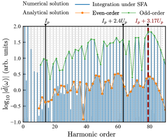
Fig. 3 presents the comparison of harmonics $|\tilde{d}(\omega)|$ from numerical integration of Eq. (1) with analytical formula, Eq. (6) and Eq. (11), for odd- and even-order harmonics, respectively, when initial phase $\phi=\pi/2$ is chosen to maximize the yield of even-order harmonics. The agreement between odd-order $|\tilde{d}(\omega)|$ evaluated by Eq. (1) with the analytical solution of Eq. (6) confirms the conclusion that the additional THz field with the current laser parameters imposes no influences on odd-order harmonic generation. On the other hand, the yields of even-order harmonics are typically lower than their odd-order counterparts due to the small ratio of frequencies $\varepsilon$ in the prefactor of Eq. (11). The derived solution of Eq. (11) is also in excellent agreement with the numerical result for NCEHs, showing the validity of the assumed conditions that only $J_{N}(z)$ of $N=\pm 1$ contribute. Eq. (11) even works in a broader parametric range than expected — it correctly describes all even-order harmonics above 40th-order, which corresponds to a much lower energy than that of the cutoff.

The above analysis establishes the basis for the generation of NCEHs. In the following, the envelope effect for a more realistic laser pulse will be presented to account for the time-resolving capacity of the femtosecond laser pulse in THz detection.

III.3 Effect of pulse envelope

The envelope of a femtosecond laser pulse should be considered in practice. It is expected that the temporal locality specified by the envelope plays an essential role in determining the waveform of the THz field at exactly the time of pulse center. In this section, we first discuss the envelope effect on harmonics in the absence of the THz field.

Assuming the vector potential has a Gaussian-envelope, $A(t)=A_{0}\exp[-t^{2}/(2\sigma^{2})]\sin(\omega_{0}t)$, with the time center at $t=0$ and the pulse width $\sigma$, the excursion of the electron is given by $\alpha(t)=-A_{0}\exp[-(\omega_{0}\sigma)^{2}/2]\sqrt{\pi/2}\sigma\mathrm{\operatorname{Im}}\left[\mathrm{\operatorname{erf}}\left(t/\sqrt{2}\sigma+\mathrm{i}\omega_{0}\sigma/\sqrt{2}\right)\right]$ with the error function $\text{erf}(z)=\left(2/\sqrt{\pi}\right)\int_{0}^{z}\exp(-t^{2})\mathrm{d}t$. Substituting into Eq. (2), we find the action

$$S_{0}(t,\tau) = I_{p}\tau+U_{p}\mathrm{e}^{-\left(\frac{t}{\sigma}\right)^{2}}\frac{\sqrt{\pi}}{2}\sigma G\left(\frac{t}{\sqrt{2}\sigma},\frac{\omega_{0}\sigma}{\sqrt{2}},\frac{\tau}{\sqrt{2}\sigma}\right)$$ (12)

where

$$G(x,y,\eta) = \mathrm{\operatorname{Re}}[\mathrm{e}^{\mathrm{i}4xy}g(x-\mathrm{i}y,\eta)-g(x,\eta)]$$

$$-\frac{\sqrt{2\pi}}{\eta}\left[\mathrm{\operatorname{Im}}\mathrm{e}^{\mathrm{i}2xy}g\left(\frac{x-\mathrm{i}y}{\sqrt{2}},\frac{\eta}{\sqrt{2}}\right)\right]^{2},$$

and

$$g(z,\eta) = w\left(\mathrm{i}\sqrt{2}z\right)-\mathrm{e}^{4\eta(z-\eta/2)}w\left(\mathrm{i}\sqrt{2}(z-\eta)\right)$$ (13)

with $w(z)$ the Faddeeva function defined by $w(z)=\exp(-z^{2})[1-\mathrm{\operatorname{erf}}(-\mathrm{i}z)]$.

Figure 4: Comparison of contributing phases in actions as a function of $\varphi_{t}$ between fields of continuous wave and of Gaussian envelope. Parameters $\varphi_{\sigma}=50$ and $\varphi_{\tau}=4$ are used which are typical for the generation of NCEHs.

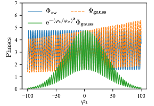
In comparison with the action for a continuous wave, Eq. (3), which can be recast as $S_{0}(\varphi_{t},\varphi_{\tau})=(I_{p}/\omega_{0})\varphi_{\tau}+(U_{p}/\omega_{0})\Phi_{\text{cw}}$ with phase $\Phi_{\text{cw}}=\varphi_{\tau}-2(1-\cos\varphi_{\tau})/\varphi_{\tau}-C_{0}(\varphi_{\tau})\cos(2\varphi_{t}-\varphi_{\tau})$, action (12) for a Gaussian-enveloped pulse takes the similar form, $S_{0}(\varphi_{t},\varphi_{\tau})=(I_{p}/\omega_{0})\varphi_{\tau}+(U_{p}/\omega_{0})\exp[-(\varphi_{t}/\varphi_{\sigma})^{2}]\Phi_{\text{gauss}}$, with $\Phi_{\text{cw}}$ replaced by a Gaussian-windowed one $\exp[-(\varphi_{t}/\varphi_{\sigma})^{2}]\Phi_{\text{gauss}}$ and $\Phi_{\text{gauss}}=\left(\sqrt{\pi}/2\right)\varphi_{\sigma}G\left(\varphi_{t}/\sqrt{2}\varphi_{\sigma},\varphi_{\sigma}/\sqrt{2},\varphi_{\tau}/\sqrt{2}\varphi_{\sigma}\right)$. Here, all notions of phases $\varphi_{t}=\omega_{0}t$ and $\varphi_{\tau}=\omega_{0}\tau$ are still used for consistency. Besides, we have introduced $\varphi_{\sigma}=\omega_{0}\sigma$. A common factor of Gaussian $\exp[-(\varphi_{t}/\varphi_{\sigma})^{2}]$ in Eq. (12) specifies a filtering window whose center coincides with that of the femtosecond pulse. A pictorial analysis on the difference of actions between the continuous wave and the Gaussian-enveloped pulse is presented in Fig. 4. The curves of both $\Phi_{\text{cw}}$ and $\Phi_{\text{gauss}}$ contain the same dominant oscillating components versus $\varphi_{t}$, proportional to $\cos(2\varphi_{t}-\varphi_{\tau})$. Within the region of interest, i.e., around the center of the Gaussian window, the difference between $\Phi_{\text{gauss}}$ and $\Phi_{\text{cw}}$ is that the oscillating amplitude of $\Phi_{\text{gauss}}$ increases with $\varphi_{t}$ while that of $\Phi_{\text{cw}}$ remains constant. Such an increase becomes more significant with decreasing $\varphi_{\sigma}$. On the contrary, when $\varphi_{\sigma}$ is sufficiently large, the amplitude of $\Phi_{\text{gauss}}$ approaches $\Phi_{\text{cw}}$. That is, when the pulse is infinitely long, i.e., $\varphi_{\sigma}\rightarrow\infty$, Eq. (12) for a Gaussian envelope degenerates to Eq. (3), the action for a monochromatic continuous wave laser.

Figure 5: Effect of pulse envelope on harmonic generation. The panels show the near-cutoff harmonics under (a) a continuous monochromatic laser of the same parameters used in Fig. 3, and (b) a Gaussian-enveloped pulse of $\sigma=1755$ (FWHM of 100 fs). The red marks label all harmonics of odd-orders, whose distribution is highlighted by orange curves. Black dashed lines indicate $E_{\text{cutoff}}$.

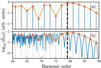
Fig. 5 shows the comparison of harmonics generations between using a continuous wave and using Gaussian-enveloped femtosecond pulse. With the same femtosecond laser parameters as considered for the continuous wave ($\omega_{0}=0.0353$, $E_{0}=0.06$), the result in Fig. 5(a) is actually a zoom-in spectrum of Fig. 3 around the near-cutoff energy, while Fig. 5(b) shows the one with a Gaussian envelope of $\sigma=100$ fs. The $|\tilde{d}(\omega)|$ at each odd-order, for either without or with envelope effect, is highlighted by orange curve, showing the similar distributions of odd-order harmonics. Action (12) modified by the finite pulse width, which has also been numerically examined, however, contains extra frequency components, leading to multiple sidebands in Fig. 5(b) around the original odd-order harmonics. In the next section the THz field combined with Gaussian-enveloped femtosecond pulse is analyzed to show the theory behind the THz field reconstruction.

III.4 THz induced NCEHs under Gaussian-enveloped pulse

The above discussions allow for a straightforward extension to consider the harmonic generation under a Gaussian-enveloped femtosecond laser pulse accompanied by a THz field. Let $A(t)=A_{0}\exp(-t^{2}/2\sigma^{2})\sin(\omega t)+A_{1}\cos(\omega_{1}t+\phi)$ be the vector potential of the combined fields. As presented in Sec. III.2, the corresponding action Eq. (7) eventually takes the form $S(t,\tau)\simeq S_{0}(t,\tau)+\Delta S(t,\tau)$, where $S_{0}(t,\tau)$ is given by Eq. (12) for a Gaussian pulse as presented in Sec. III.3, while the correction $\Delta S(t,\tau)$ derives from the cross term $-p_{\text{st},0}p_{\text{st},1}\tau+\int_{t-\tau}^{t}A_{0}(t^{\prime})A_{1}(t^{\prime})\mathrm{d}t^{\prime}$. Similar to Sec. III.2, denoting the ratio between frequencies $\varepsilon=\omega_{1}/\omega_{0}$, solving $\Delta S(t,\tau)$ yields

$$\Delta S(t,\tau) = -\frac{A_{0}A_{1}}{2}\sqrt{\frac{\pi}{2}}\sigma\mathrm{e}^{-\left(\frac{t}{\sqrt{2}\sigma}\right)^{2}}\mathrm{\operatorname{Im}}[\mathrm{e}^{\mathrm{i}\varphi_{t}}K(\varphi_{t},\varphi_{\sigma},\varphi_{\tau})],$$

where

$$K(\varphi_{t},\varphi_{\sigma},\varphi_{\tau}) = 2\cos\left[\varepsilon\left(\varphi_{t}-\frac{\varphi_{\tau}}{2}\right)+\phi\right]\mathrm{\operatorname{sinc}\left(\varepsilon\frac{\varphi_{t}}{2}\right)}g_{0}$$

$$-\mathrm{e}^{-\mathrm{i}(\varepsilon\varphi_{t}+\phi)}g_{+}-\mathrm{e}^{+\mathrm{i}(\varepsilon\varphi_{t}+\phi)}g_{-}$$

with $g_{0}\equiv g\left(z/\sqrt{2},\eta/\sqrt{2}\right)$ and $g_{\pm}\equiv g\left(z/\sqrt{2}\pm\mathrm{i}\varepsilon\varphi_{\sigma}/2,\eta/\sqrt{2}\right)$ defined by function $g(z,\eta)$ of Eq. (13). Here, arguments $z$ and $\eta$ are dimensionless compositions of time variables, $z=(\varphi_{t}/\varphi_{\sigma}-\mathrm{i}\varphi_{\sigma})/\sqrt{2}$ and $\eta=\varphi_{\tau}/\sqrt{2}\varphi_{\sigma}$. With a small $\varepsilon$, the series expansion of $K(\varphi_{t},\varphi_{\sigma},\varphi_{\tau})$ with respect to $\varepsilon$ up to the first order results in

$$K(\varphi_{t},\varphi_{\sigma},\varphi_{\tau}) \simeq -2\sqrt{2}\varepsilon\mathrm{e}^{\mathrm{i}\varphi_{t}}\varphi_{\sigma}\sin\phi\Xi(z,\eta),$$

where

$$\Xi(z,\eta) = \left(z-\frac{\eta}{2}\right)g\left(\frac{z}{\sqrt{2}},\frac{\eta}{\sqrt{2}}\right)-\frac{1-\mathrm{e}^{2\eta\left(z-\frac{\eta}{2}\right)}}{\sqrt{\pi}}.$$

Hence the action is given by

$$\Delta S(t,\tau) \simeq \sqrt{\pi}A_{0}E_{1}\mathrm{e}^{-\left(\frac{\varphi_{t}}{\sqrt{2}\varphi_{\sigma}}\right)^{2}}\sin\phi\sigma^{2}\mathrm{\operatorname{Im}}[\mathrm{e}^{\mathrm{i}\varphi_{t}}\Xi(z,\eta)].$$ (14)

With a typically large value of $\varphi_{\sigma}$ when the femtosecond laser of several tens of optical cycles is used, the Faddeeva function $w(z)\simeq\mathrm{i}z/\sqrt{\pi}(z^{2}-1/2)$ if $|z|^{2}\geqslant 256$ Zaghloul (2017). Using the approximation and explicitly expanding the imaginary part in $\Delta S(t,\tau)$, the full expression can be rearranged by trigonometric functions, whose coefficients, each as a polynomial of time variables, can be further simplified by retaining only the highest order of $\varphi_{\sigma}$. Eventually, we find

$$\Delta S(t,\tau) \simeq \frac{A_{0}E_{1}}{2\omega_{0}^{2}}\mathrm{e}^{-\left(\frac{\varphi_{t}}{\sqrt{2}\varphi_{\sigma}}\right)^{2}}\sin\phi\{-\varphi_{\tau}\cos\varphi_{t}+2\sin\varphi_{t}$$

$$-\mathrm{e}^{\frac{\varphi_{t}\varphi_{\tau}}{\varphi_{\sigma}^{2}}}[\varphi_{\tau}\cos(\varphi_{t}-\varphi_{\tau})+2\sin(\varphi_{t}-\varphi_{\tau})\}.$$

When the pulse duration is sufficiently long, $\exp(\varphi_{t}\varphi_{\tau}/\varphi_{\sigma}^{2})\simeq 1$, $\Delta S(t,\tau)$ approaches

$$\Delta S(t,\tau) \simeq -\frac{A_{0}E_{1}}{\omega_{0}^{2}}\mathrm{e}^{-\frac{\varphi_{t}^{2}}{2\varphi_{\sigma}^{2}}}\sin\phi C_{1}(\varphi_{\tau})\cos\left(\varphi_{t}-\frac{\varphi_{\tau}}{2}\right),$$ (15)

recovering action (8) under continuous waves as discussed in Sec. III.2, except for the presence of an extra prefactor $\exp(-t^{2}/2\sigma^{2})$ that serves as a temporal window.

Figure 6: Comparison of $|\tilde{d}(\omega)|$ evaluated by direct numerical integration of Eq. (1) (blue) and by using the derived action, $S=S_{0}+\Delta S$, with $S_{0}$ and $\Delta S$ given by Eqs. (12) and (15), respectively. The same parameters of femtosecond pulse as in Fig. 5 are used except for $\sigma=2106$ (FWHM of 120 fs). The THz field is parametrized by $\omega_{1}=1\times 10^{-4}$, $E_{1}=2\times 10^{-5}$ and $\phi=\pi/2$.

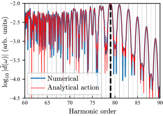
Fig. 6 shows the comparison of near-cutoff harmonics evaluated by direct numerical integration of Eq. (1) with that obtained by applying the action of analytical form, $S(t,\tau)=S_{0}(t,\tau)+\Delta S(t,\tau)$, with $S_{0}(t,\tau)$ and $\Delta S(t,\tau)$ given by Eqs. (12) and (15), respectively. The comparison presents a rather good agreement, justifying the analytically derived action with the assumed approximations. Comparing with harmonics in Fig. 5(b) without THz field, it is shown that the odd-order harmonics are dominantly determined by $S_{0}(t,\tau)$, as those harmonics in both Fig. 5(b) and Fig. 6 are almost the same, though odd-order harmonic peaks in the latter are slightly sharper due to the use of longer pulse width of the femtosecond laser. In Fig. 6, however, NCEHs emerge, clearly indicating that even-order harmonics originate from the THz-induced correction $\Delta S(t,\tau)$.

From Eq. (15), following the similar procedure of analysis in Sec. III.2, the reasoning behind the generation of NCEHs in an enveloped laser pulse is straightforward. Within the temporal window specified by the Gaussian envelope, the strength of NCEHs is approximately proportional to THz field strength exactly at the center of the envelope. In other words, under the influence of the THz field that induces even-order harmonics, the femtosecond pulse with a filtering temporal window maps the instantaneous strength of THz field onto that of NCEHs, allowing for a complete characterization of the THz time-domain spectrum with the femtosecond pulse scanning over the THz field.

Figure 7: Near cut-off harmonics without THz field (blue) and with THz field (orange) when (a) $\phi=\pi/2$ and (b) $\phi=\pi$. The inset of each panel shows the time center of femtosecond pulse (blue) relative to that of the THz field (orange) for different $\phi$. Marks "$\circ$" (“$\times$”) label the even-order harmonics with (without) the THz field. The position of $E_{\text{cutoff}}$ is indicated by the black dashed line. The same parameters as in Fig. 6 are used.

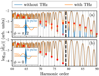
Fig. 7 shows the dependence of NCEHs on initial phase $\phi$, or equivalently, the pulse center of the femtosecond laser relative to the electric component of the THz field. When $\phi=\pi/2$, factor $\sin\phi=1$ in Eq. (15) maximizes the coefficient of NCEHs as analyzed in Eq. (11). As shown in Fig. 7(a), the even-order harmonics under a THz field is significantly higher than its counterpart without the THz field, and the amplitude relative to their adjacent odd-order harmonics becomes even more significant when the order approaching the cutoff. On the contrary, in Fig. 7(b), when $\phi=0$, the even-order harmonics vanish and the harmonic distribution in the presence of THz field is exactly the same as the one without the THz field. Except for even-order harmonics, the harmonics of other energies are almost identical between panels (a) and (b), showing they are barely influenced by the THz field. As indicated by insets of Fig. 7, at $\phi=\pi/2$ ($\phi=0$), the center of the femtosecond pulse is at the maximum (the zero-point) of the THz electric field. The coincidence of the NCEHs yields with the THz electric field shows the feasibility to reconstruct the latter using the former.

Figure 8: Reconstruction of time-domain spectrum of THz waves. (a) The parameters are the same as used in Fig. 1. $\omega_{0}=0.0353$ (1.3 $\mu$m), $E_{0}=0.06$ ($I=1.3\times 10^{14}$ W/cm²), $\sigma=2106$ (FWHM of 120 fs), $\omega_{1}=2\times 10^{-4}$ (1 THz), and $E_{1}=2\times 10^{-5}$ (100 kV/cm). (b) The reconstruction for THz wave of higher frequency with $\omega_{0}=0.1139$ (400 nm), $E_{0}=0.06$ ($I=1.3\times 10^{14}$ W/cm²), $\sigma=702$ (FWHM of 40 fs), $\omega_{1}=0.003$ (20 THz), and $E_{1}=2\times 10^{-5}$ (100 kV/cm). Insets show the temporal profiles $E_{0}(t)$ and $E_{1}(t)$ of the femtosecond pulse and the THz field, respectively.

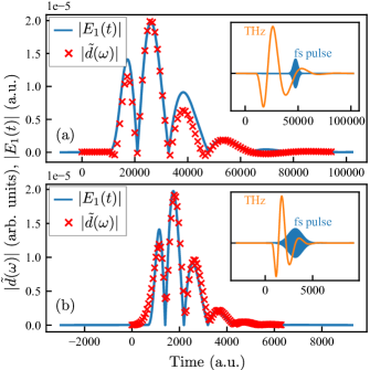
In Fig. 8, the reconstruction of THz field from the NCEHs is demonstrated by examples. Changing the time delay between the femtosecond pulse and the THz field, the even-order harmonic nearest to the cutoff on the lower energy side is retrieved and compared with $|E_{1}(t)|$ of the THz field. Using the same parameters of fields as mentioned above, we present the reconstruction with the 78th-order NCEH in Fig. 8(a), which in general shows a good agreement of $|d(\omega)|$ with $|E_{1}(t)|$. Another example to detect the THz field of higher frequency is presented in (b) to show the universality of the scheme. In order to resolve the THz field of 20 THz, a femtosecond pulse of higher frequency is required to ensure a low ratio $\varepsilon=\omega_{1}/\omega_{0}$. Using a 400 nm laser pulse with $\varepsilon\simeq 0.03$ and reducing the pulse width to 40 fs, the generated 6th-order harmonic can also be used to reveal the time-domain THz wave. The successful reconstruction of THz wave of short-time scale suggests the possibility of THz broadband detection under the aid of the NCEHs measurement.

The applicability of the reconstruction scheme is closely related to the approximations applied for the analysis in previous sections. From the temporal perspective, $\varepsilon=\omega_{1}/\omega_{0}\ll 1$ is a must, indicating that the characterization of THz field of high frequency needs high frequency femtosecond pulse. Moreover, the approximation of Faddeeva function to solve Eq. (14) requires $(\varphi_{t}^{2}/\varphi_{\sigma}^{2}+\varphi_{\sigma}^{2})/2>256$, necessitating $\varphi_{\sigma}>23$, suggesting a femtosecond pulse should contain as least 9 cycles within its FWHM. The range of $\varphi_{\sigma}$ also naturally satisfies both conditions that $\eta=\varphi_{\tau}/\varphi_{\sigma}\ll 1$ and $\exp(\varphi_{t}\varphi_{\tau}/\varphi_{\sigma}^{2})\simeq 1$ to derive (15). In general, the scheme favors the use of large $\varphi_{\sigma}$, which also helps suppress the sideband caused by the finite pulse width. Nevertheless, a smaller $\varphi_{\sigma}$ allows for a better time resolution of the waveform reconstruction. Therefore, a balance inbetween should be considered for the choice of $\varphi_{\sigma}$, which also depends on the frequency range of THz field to detect.

In addition, the choice of laser parameters, including field amplitudes $E_{0}$, $E_{1}$ and frequency $\omega_{0}$, is critical to the applicability of the reconstruction scheme. The small value of the argument of the Bessel function in Eq. (10) imposes the condition $|\varepsilon(A_{0}A_{1}/\omega_{0})C_{1}(\varphi_{\tau})|=|(E_{0}E_{1}/\omega_{0}^{3})C_{1}(\varphi_{\tau})|<1$. As shown in Fig. 4, the value of $|C_{1}(\varphi_{\tau})|\in[1.7,5.2]$ when $\varphi_{\tau}\in[3,5]$ for near-cutoff harmonics allows for an estimation of the loosely restricting criterion, $E_{0}E_{1}/\omega_{0}^{3}<0.2$. Moreover, neglecting the THz field $E_{1}(t)$ in the prefactor of dipole matrix elements, $\mu^{\ast}[p_{\operatorname{st}}(\varphi_{t},\varphi_{\tau})+A(\varphi_{t})]\mu[p_{\operatorname{st}}(\varphi_{t},\varphi_{\tau})+A(\varphi_{t}-\varphi_{\tau})]E(\varphi_{t}-\varphi_{\tau})$, requires $E_{1}\ll E_{0}$. Both conditions indicate an upper limit for $E_{1}$. That is, the detected THz field in this work is not supposed to be overwhelmingly intense, otherwise the approximation of the Bessel function in Eq. (10) breaks down, resulting in nonvanishing high-order components that contribute to other complicated effects accompanied by a strong low-frequency field, e.g., the field-induced multi-plateau structure. Since the theory works in the tunneling regime, $I_{p}\leqslant 2U_{p}$, the femtosecond laser also satisfies $E_{0}^{2}>2\omega_{0}^{2}I_{p}$.

Besides the conditions required to justify the reconstruction scheme, we also need to take the finite signal-to-noise ratio into account. The even-order harmonics should be large enough to observe. Assuming the amplitude of even-order harmonics to the adjacent odd-order one is no less than one percent, we may impose an extra condition with the coefficients of harmonics, $\varepsilon A_{0}A_{1}/2\omega_{0}=E_{0}E_{1}/2\omega_{0}^{3}>10^{-2}$, yielding $E_{0}E_{1}/\omega_{0}^{3}>0.02$. In contrast to the condition specified by the approximation of Bessel function, it indicates the field amplitudes should be large enough to generate even-order harmonics.

Figure 9: Available parametric range for THz reconstruction with NCEHs with regard to frequency $\omega_{0}$ and field amplitudes $E_{0}$ and $E_{1}$. The detailed conditions are specified in the main text.

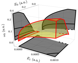
All above conditions for the reconstruction scheme can be pictorially illustrated in the parametric space as shown in Fig. 9, where the appropriate parametric range is highlighted. When $E_{1}$ of the THz field is low, a femtosecond pulse of longer wavelength avails the measurement; on the contrary, the THz field of increasing $E_{1}$ requires a femtosecond pulse of higher $\omega_{0}$, whose optional frequency range also becomes broader. Concerning the relation $\varepsilon=\omega_{1}/\omega_{0}\ll 1$, the accessible frequency of the THz field for waveform reconstruction thus depends on field amplitudes. Especially both $E_{0}$ and $E_{1}$ being high favors the use of higher $\omega_{0}$, allowing for the detection of THz field of higher $\omega_{1}$.

IV Summary and conclusion

The harmonic generation by a half-wave symmetric driving laser that interacts with isotropic media has long been known to yield odd-order harmonics only Ben-Tal et al. (1993). The emergence of even-order harmonics usually attributes to certain broken symmetries Neufeld et al. (2019), e.g., the THz field induced broken symmetry in this work. Here, the even-order harmonic generation near the cutoff is found to have a particularly synchronous relation with the THz electric field. The analytical derivation with perturbative expansion shows the NCEHs originate from the first-order correction with regard to the ratio between frequencies of the THz field and that of the femtosecond laser pulse. The linear relation between the NCEH amplitude and the THz electric field derives from an approximation of the Bessel function, which can be fulfilled by the specific range of return time corresponding to the near-cutoff energy region.

The direct mapping from the THz field to NCEHs thus provides an alternative conceptually simple approach to reconstruct time-domain THz wave from NCEHs. The proposal to measure NCEHs as a function of the time delay between the femtosecond laser pulse and the THz field has been numerically verified, showing the applicability of the method for the broadband THz detection. The analytical derivations also help identify the parametric region for such applications, indicating high-frequency THz field characterization should require higher laser intensity. The encoding of the time-domain information of THz wave into NCEHs may inspire new routes towards the realization of coherent detection in broad spectral range.