11institutetext: Elias S. Helou, Instituto de Ciências Matemáticas e de Computação, elias@icmc.usp.br
Marcelo V. W. Zibetti, Center for Advanced Imaging Innovation and Research (CAI2R), New York University School of Medicine, Marcelo.WustZibetti@nyumc.org
Gabor T. Herman, PhD Program in Computer Science, City University of New York, gabortherman@yahoo.com

Fast Proximal Gradient Methods for Nonsmooth Convex Optimization for Tomographic Image Reconstruction

Elias S. Helou    Marcelo V. W. Zibetti    and Gabor T. Herman
Abstract

The Fast Proximal Gradient Method (FPGM) and the Monotone FPGM (MFPGM) for minimization of nonsmooth convex functions are introduced and applied to tomographic image reconstruction. Convergence properties of the sequence of objective function values are derived, including a O(1/k2)𝑂1superscript𝑘2O\left(1/k^{2}\right) non-asymptotic bound. The presented theory broadens current knowledge and explains the convergence behavior of certain methods that are known to present good practical performance. Numerical experimentation involving computerized tomography image reconstruction shows the methods to be competitive in practical scenarios. Experimental comparison with Algebraic Reconstruction Techniques are performed uncovering certain behaviors of accelerated Proximal Gradient algorithms that apparently have not yet been noticed when these are applied to tomographic image reconstruction.
Keywords Computerized tomography imaging, Convex optimization, Proximal gradient methods, Iterative algorithms.
Mathematics Subject Classification 65K05, 68U10, 90C25, 90C06, 92C55, 94A08

1 Introduction

In this paper we introduce the Fast Proximal Gradient Methods (FPGM) for the solution of convex minimization problems of the form

minΨ(𝐱):=f(𝐱)+ϕ(𝐱),assignΨ𝐱𝑓𝐱italic-ϕ𝐱\min\quad\Psi(\mathbf{x}):=f(\mathbf{x})+\phi(\mathbf{x}), (1)

where f:n:𝑓superscript𝑛f:\mathbb{R}^{n}\to\mathbb{R} is a smooth convex function with Lipschitz continuous gradient and ϕ:n:italic-ϕsuperscript𝑛\phi:\mathbb{R}^{n}\to\mathbb{R} is a proper convex function. It is not assumed that ϕitalic-ϕ\phi is smooth. From now on, the symbols f𝑓f and ϕitalic-ϕ\phi will always represent functions satisfying these assumptions.

Many practical problems fit this general model. In particular, for image reconstruction from tomographic data, f(𝒙)𝑓𝒙f(\boldsymbol{x}) is usually going to be a measure of consistency, according to the data acquisition model, of image 𝒙𝒙\boldsymbol{x} with the data coming from the scanner whereas ϕ(𝒙)italic-ϕ𝒙\phi(\boldsymbol{x}) is a measure of structure. For example, ϕitalic-ϕ\phi could enforce sparsity, smoothness, or some other desirable a priori information known about the image being reconstructed.

The algorithms we propose here lie between the Optimized Iterative Shrinkage-Thresholding Algorithm (OISTA) presented and experimented with in Kim and Fessler (2016), but for which no convergence proof exists, and the Overrelaxed Monotone Fast Iterative Shrinkage-Thresholding Algorithm (OMFISTA) Yamagishi and Yamada (2011), for which convergence proofs do exist. One contribution of the present paper is a better understanding of the convergence properties of these algorithms. We get there by increasing the range of allowed parameters values for OMFISTA, consequently providing a way of justifying convergence of OISTA. We exhibit numerical experimentation using FPGM for computerized tomography image reconstruction Herman (2009) with both real and synthetic data and compare it with other methods from the viewpoint of convergence speed and image quality.

The paper is organized as follows. The remaining of the present section is dedicated to introduce the mathematical elements that will be used in the construction of the algorithm. Section 2 contains a non-extensive literature review about the subject of fast proximal gradient methods and fast first-order methods. The new algorithm is introduced in Section 3 and its convergence is analyzed in Section 4. Numerical experiments are presented in Section 5. Finally, Section 6 brings our conclusions and delineates plans for future work.

1.1 Proximal Operators

Proximal operators are useful tools for convex optimization, presenting an interesting balance between abstract power and practical applicability. Given a proper convex function ϕ:n:italic-ϕsuperscript𝑛\phi:\mathbb{R}^{n}\to\mathbb{R} and a positive real number L𝐿L, the L𝐿L-proximal point of ϕitalic-ϕ\phi from a point 𝐱n𝐱superscript𝑛\mathbf{x}\in\mathbb{R}^{n} is defined as:

proxϕ,L(𝐱):=argmin𝐲n{ϕ(𝐲)+L2𝐲𝐱2}.assignsubscriptproxitalic-ϕ𝐿𝐱subscriptargmin𝐲superscript𝑛italic-ϕ𝐲𝐿2superscriptnorm𝐲𝐱2\operatorname*{prox}_{\phi,L}(\mathbf{x}):=\operatorname*{arg\,min}_{\mathbf{y}\in\mathbb{R}^{n}}\left\{\phi(\mathbf{y})+\frac{L}{2}\left\|\mathbf{y}-\mathbf{x}\right\|^{2}\right\}. (2)

We will, when there is no risk of confusion, refer to the L𝐿L-proximal point of ϕitalic-ϕ\phi from 𝐱n𝐱superscript𝑛\mathbf{x}\in\mathbb{R}^{n} simply as the proximal point.

Although the computation of the proximal point involves a minimization, in many cases of interest this computation can be performed in a finite number of simple steps. Examples of functions ϕitalic-ϕ\phi that allow efficient closed-form representations of proxϕ,Lsubscriptproxitalic-ϕ𝐿\operatorname*{prox}_{\phi,L} include the 1subscript1\ell_{1} norm of an orthonormal transformation of a vector, that is, ϕ(𝐱)=Q𝐱1italic-ϕ𝐱subscriptnorm𝑄𝐱1\phi(\mathbf{x})=\left\|Q\mathbf{x}\right\|_{1} where Qn×n𝑄superscript𝑛𝑛Q\in\mathbb{C}^{n\times n} with QQ=Isuperscript𝑄𝑄𝐼Q^{*}Q=I, and the nuclear norm of a matrix Mm×n𝑀superscript𝑚𝑛M\in\mathbb{C}^{m\times n}, i.e., ϕ(M)=M=i=1min{m,n}|σi|italic-ϕ𝑀subscriptnorm𝑀superscriptsubscript𝑖1𝑚𝑛subscript𝜎𝑖\phi(M)=\left\|M\right\|_{*}=\sum_{i=1}^{\min\{m,n\}}|\sigma_{i}|, where the σisubscript𝜎𝑖\sigma_{i} are the singular values of M𝑀M. For some other important functions, such as the Total Variation (TV𝑇𝑉TV), there are effective iterative procedures than can quickly approximate proxϕ,L(𝐱)subscriptproxitalic-ϕ𝐿𝐱\operatorname*{prox}_{\phi,L}(\mathbf{x}) Beck and Teboulle (2009b).

1.2 Proximal Gradient Methods

Let us define the proximal gradient operator as:

PL,f,ϕ(𝐱):=proxϕ,L(𝐱1Lf(𝐱)).assignsubscript𝑃𝐿𝑓italic-ϕ𝐱subscriptproxitalic-ϕ𝐿𝐱1𝐿𝑓𝐱P_{L,f,\phi}(\mathbf{x}):=\operatorname*{prox}_{\phi,L}\left(\mathbf{x}-\frac{1}{L}\nabla f(\mathbf{x})\right). (3)

For simplicity, we will omit f𝑓f and ϕitalic-ϕ\phi from the notation unless the omission causes ambiguity. A Proximal Gradient Method (PGM) for the minimization of (1) is then given by an iterative process in which

𝐱k+1=PL(𝐱k),subscript𝐱𝑘1subscript𝑃𝐿subscript𝐱𝑘\mathbf{x}_{k+1}=P_{L}\left(\mathbf{x}_{k}\right), (4)

see Parikh and Boyd (2014). For large enough L𝐿L, these iterations converge, but they do so slowly, and rates of the kind Ψ(𝐱k)Ψ(𝐱)=O(1/k)Ψsubscript𝐱𝑘Ψsuperscript𝐱𝑂1𝑘\Psi(\mathbf{x}_{k})-\Psi(\mathbf{x}^{*})=O\left(1/k\right), where 𝐱nsuperscript𝐱superscript𝑛\mathbf{x}^{*}\in\mathbb{R}^{n} is a minimizer of ΨΨ\Psi, are often predicted theoretically and observed in practice.

For smooth problems of the form

minf(𝐱),𝑓𝐱\min\quad f(\mathbf{x}), (5)

Nesterov Nesterov (1983) introduced the Fast Gradient Method (FGM)

𝐱k=𝐲k1Lf(𝐲k),subscript𝐱𝑘subscript𝐲𝑘1𝐿𝑓subscript𝐲𝑘\mathbf{x}_{k}=\mathbf{y}_{k}-\frac{1}{L}\nabla f\left(\mathbf{y}_{k}\right), (6)

where 𝐲1=𝐱0subscript𝐲1subscript𝐱0\mathbf{y}_{1}=\mathbf{x}_{0} and

𝐲k+1=𝐱k+tk1tk+1(𝐱k𝐱k1),subscript𝐲𝑘1subscript𝐱𝑘subscript𝑡𝑘1subscript𝑡𝑘1subscript𝐱𝑘subscript𝐱𝑘1\mathbf{y}_{k+1}=\mathbf{x}_{k}+\frac{t_{k}-1}{t_{k+1}}\left(\mathbf{x}_{k}-\mathbf{x}_{k-1}\right), (7)

with t1=1subscript𝑡11t_{1}=1 and tk=(1+1+4tk12)/2subscript𝑡𝑘114superscriptsubscript𝑡𝑘122t_{k}=\left(1+\sqrt{1+4t_{k-1}^{2}}\right)/2. Later, Beck and Teboulle proved that the same algorithmic form leads to a fast proximal gradient algorithm, called Fast Iterative Shrinkage-Thresholding Algorithm (FISTA) Beck and Teboulle (2009a, b), when (6) is replaced by

𝐱k=PL(𝐲k).subscript𝐱𝑘subscript𝑃𝐿subscript𝐲𝑘\mathbf{x}_{k}=P_{L}\left(\mathbf{y}_{k}\right). (8)

These fast algorithms have much better theoretical and practical convergence properties than a PGM, at only a small extra computational cost, specially in high-dimensional problems such as occur in computerized tomography image reconstruction Herman (2009).

2 Literature Review

The introduction of FISTA renewed interest in Nesterov’s ideas because the separable smooth plus nonsmooth model has a wider application range than smooth minimization, including many image processing and reconstruction problems within the Compressive Sensing (CS) framework Donoho (2006). Nesterov introduced his seminal ideas by considering First-Order Methods (FOMs) for the solution of (5). A FOM is a method with an iterative step of the form:

𝐱k+1=𝐱k1Li=0khk+1,if(𝐱i),subscript𝐱𝑘1subscript𝐱𝑘1𝐿superscriptsubscript𝑖0𝑘subscript𝑘1𝑖𝑓subscript𝐱𝑖\mathbf{x}_{k+1}=\mathbf{x}_{k}-\frac{1}{L}\sum_{i=0}^{k}h_{k+1,i}\nabla f\left(\mathbf{x}_{i}\right), (9)

where hk+1,isubscript𝑘1𝑖h_{k+1,i}\in\mathbb{R} for k𝑘k\in\mathbb{N} and i{0,1,,k}𝑖01𝑘i\in\{0,1,\dots,k\}. For this class of methods, there is a smooth convex function f𝑓f with Lipschitz continuous gradient such that the sequence of iterates of every FOM would satisfy Nesterov (2004)

f(𝐱k)f(𝐱)3L𝐱0𝐱232(k+1)2,𝑓subscript𝐱𝑘𝑓superscript𝐱3𝐿superscriptnormsubscript𝐱0superscript𝐱232superscript𝑘12f(\mathbf{x}_{k})-f(\mathbf{x}^{*})\geq\frac{3L\left\|\mathbf{x}_{0}-\mathbf{x}^{*}\right\|^{2}}{32(k+1)^{2}}, (10)

thereby establishing a lower bound for the worst case scenario. On the other hand, the optimality gap, that is, the difference between the objective function value at the current iteration and the optimal objective function value, of the FGM was shown to be bounded by

f(𝐱k)f(𝐱)2L𝐱0𝐱2(k+1)2.𝑓subscript𝐱𝑘𝑓superscript𝐱2𝐿superscriptnormsubscript𝐱0superscript𝐱2superscript𝑘12f(\mathbf{x}_{k})-f(\mathbf{x}^{*})\leq\frac{2L\left\|\mathbf{x}_{0}-\mathbf{x}^{*}\right\|^{2}}{(k+1)^{2}}. (11)

Since FGM is a FOM, this algorithm has a convergence rate in terms of reduction of the objective function value with optimal leading exponent. However, the difference between the coefficients in the bounds (10) and (11) left hope for improvement of the convergence rate of FOMs.

More recently, Kim and Fessler Kim and Fessler (2016) refined an approach by Drori and Teboulle Drori and Teboulle (2014) and obtained a method called Optimized Gradient Method (OGM) with the proven property that

f(𝐱k)f(𝐱)L𝐱0𝐱2(k+1)2,𝑓subscript𝐱𝑘𝑓superscript𝐱𝐿superscriptnormsubscript𝐱0superscript𝐱2superscript𝑘12f(\mathbf{x}_{k})-f(\mathbf{x}^{*})\leq\frac{L\left\|\mathbf{x}_{0}-\mathbf{x}^{*}\right\|^{2}}{(k+1)^{2}}, (12)

with iterations given by

𝐱k=𝐲k1Lf(𝐲k),subscript𝐱𝑘subscript𝐲𝑘1𝐿𝑓subscript𝐲𝑘\mathbf{x}_{k}=\mathbf{y}_{k}-\frac{1}{L}\nabla f\left(\mathbf{y}_{k}\right), (13)
𝐲k+1=𝐱k+tk1tk+1(𝐱k𝐱k1)+tktk+1(𝐱k𝐲k).subscript𝐲𝑘1subscript𝐱𝑘subscript𝑡𝑘1subscript𝑡𝑘1subscript𝐱𝑘subscript𝐱𝑘1subscript𝑡𝑘subscript𝑡𝑘1subscript𝐱𝑘subscript𝐲𝑘\mathbf{y}_{k+1}=\mathbf{x}_{k}+\frac{t_{k}-1}{t_{k+1}}\left(\mathbf{x}_{k}-\mathbf{x}_{k-1}\right)+\frac{t_{k}}{t_{k+1}}\left(\mathbf{x}_{k}-\mathbf{y}_{k}\right). (14)

The generalization of FGM to the nonsmooth case came when Beck and Teboulle Beck and Teboulle (2009a) showed that the gradient step can be replaced by a proximal gradient step leading to the FISTA

𝐱k=PL(𝐲k),subscript𝐱𝑘subscript𝑃𝐿subscript𝐲𝑘\mathbf{x}_{k}=P_{L}\left(\mathbf{y}_{k}\right), (15)
𝐲k+1=𝐱k+tk1tk+1(𝐱k𝐱k1).subscript𝐲𝑘1subscript𝐱𝑘subscript𝑡𝑘1subscript𝑡𝑘1subscript𝐱𝑘subscript𝐱𝑘1\mathbf{y}_{k+1}=\mathbf{x}_{k}+\frac{t_{k}-1}{t_{k+1}}\left(\mathbf{x}_{k}-\mathbf{x}_{k-1}\right). (16)

FISTA, similarly to FGM, satisfies

Ψ(𝐱k)Ψ(𝐱)2L𝐱0𝐱2(k+1)2.Ψsubscript𝐱𝑘Ψsuperscript𝐱2𝐿superscriptnormsubscript𝐱0superscript𝐱2superscript𝑘12\Psi(\mathbf{x}_{k})-\Psi(\mathbf{x}^{*})\leq\frac{2L\left\|\mathbf{x}_{0}-\mathbf{x}^{*}\right\|^{2}}{(k+1)^{2}}. (17)

A monotone version of FISTA, called MFISTA was also developed Beck and Teboulle (2009b), which shares with FISTA the same bound on the optimality gap. Kim and Fessler successfully experimented with a version of the OGM where the gradient step is replaced by the proximal gradient step Kim and Fessler (2015). Although numerically the algorithm so obtained behaved well, no theoretical convergence proof was provided.

In the present paper we prove convergence of algorithms of the form

𝐱k=PLk(𝐲k),subscript𝐱𝑘subscript𝑃subscript𝐿𝑘subscript𝐲𝑘\mathbf{x}_{k}=P_{L_{k}}\left(\mathbf{y}_{k}\right), (18)
𝐲k+1=𝐱k+tk1tk+1(𝐱k𝐱k1)+tktk+1(ηk1)(𝐱k𝐲k).subscript𝐲𝑘1subscript𝐱𝑘subscript𝑡𝑘1subscript𝑡𝑘1subscript𝐱𝑘subscript𝐱𝑘1subscript𝑡𝑘subscript𝑡𝑘1subscript𝜂𝑘1subscript𝐱𝑘subscript𝐲𝑘\mathbf{y}_{k+1}=\mathbf{x}_{k}+\frac{t_{k}-1}{t_{k+1}}\left(\mathbf{x}_{k}-\mathbf{x}_{k-1}\right)+\frac{t_{k}}{t_{k+1}}\left(\eta_{k}-1\right)\left(\mathbf{x}_{k}-\mathbf{y}_{k}\right). (19)

Under suitable conditions on the sequence {ηk}subscript𝜂𝑘\{\eta_{k}\}\subset\mathbb{R}, convergence can be proven to follow

Ψ(𝐱k)Ψ(𝐱)2Lk𝐱0𝐱2ηk(k+1)2.Ψsubscript𝐱𝑘Ψsuperscript𝐱2subscript𝐿𝑘superscriptnormsubscript𝐱0superscript𝐱2subscript𝜂𝑘superscript𝑘12\Psi(\mathbf{x}_{k})-\Psi(\mathbf{x}^{*})\leq\frac{2L_{k}\left\|\mathbf{x}_{0}-\mathbf{x}^{*}\right\|^{2}}{\eta_{k}(k+1)^{2}}. (20)

Notice that for ηk=2subscript𝜂𝑘2\eta_{k}=2 the 𝐲ksubscript𝐲𝑘\mathbf{y}_{k} update in (19) is the same than the one of OGM and the above convergence bound also equals the one for OGM. It appears not to be possible, however, to prove convergence of algorithm (18)-(19) with ηk2subscript𝜂𝑘2\eta_{k}\equiv 2 for every problem Taylor et al. (2017). Instead, in our approach a valid range of values for the coefficient ηksubscript𝜂𝑘\eta_{k} is computed during the execution of iteration k𝑘k of the algorithm, but we noticed that in practice the upper bound of this range is often larger than 222, allowing, for example, us to often use ηk2subscript𝜂𝑘2\eta_{k}\approx 2 and thus to make (19) approximately equal to (14).

A similar method is the generalization of FISTA called OMFISTA Yamagishi and Yamada (2011). The convergence theory provided for OMFISTA was valid only in the range ηk(0,1]subscript𝜂𝑘01\eta_{k}\in(0,1], and so did not include the case ηk=2subscript𝜂𝑘2\eta_{k}=2 that characterizes OISTA. In Zibetti et al. (2019), monotone FISTA with variable acceleration (MFISTA-VA) is proposed, and it is shown that an ηk>2subscript𝜂𝑘2\eta_{k}>2 may be chosen when the new iterate 𝐱ksubscript𝐱𝑘\mathbf{x}_{k} satisfies Ψ(𝐱k)<Ψ(PLk(𝐲k))Ψsubscript𝐱𝑘Ψsubscript𝑃subscript𝐿𝑘subscript𝐲𝑘\Psi\left(\mathbf{x}_{k}\right)<\Psi\left(P_{L_{k}}\left(\mathbf{y}_{k}\right)\right), which may lead to an extra algorithmic step and variable acceleration. Here we generalize what is proposed in Zibetti et al. (2019) and prove that similar bounds can be achieved when (18) is used, thereby making our results relevant to the convergence of OISTA.

All of the above approaches speed up the Iterative Soft Thresholding Algorithm (ISTA), which has iterations of the form 𝐱k+1=PL(𝐱k)subscript𝐱𝑘1subscript𝑃𝐿subscript𝐱𝑘\mathbf{x}_{k+1}=P_{L}\left(\mathbf{x}_{k}\right), using a momentum term that considers previous iterates when updating the current iterate. Another such approach, based on a different insight than Nesterov’s, is the Two-Step Iterative Soft Thresholding (TwIST) Bioucas-Dias and Figueiredo (2007) method. TwIST can be applied to problems of the form

min12K𝐱𝒃2+ϕ(𝐱)12superscriptnorm𝐾𝐱𝒃2italic-ϕ𝐱\min\quad\frac{1}{2}\|K\mathbf{x}-\boldsymbol{b}\|^{2}+\phi(\mathbf{x}) (21)

and is considerably faster than IST in the case of poorly conditioned invertible operators K𝐾K. TwIST is inspired by a two-step method for the solution of the linear system of equations K𝒙=𝒃𝐾𝒙𝒃K\boldsymbol{x}=\boldsymbol{b} and is obtained by replacing appearances of a scaled version of the gradient f𝑓\nabla f of f(𝒙)=12K𝐱𝒃2𝑓𝒙12superscriptnorm𝐾𝐱𝒃2f(\boldsymbol{x})=\frac{1}{2}\|K\mathbf{x}-\boldsymbol{b}\|^{2} in that algorithm by the proximal-gradient operator PLsubscript𝑃𝐿P_{L}.

SpaRSA (Sparse Reconstruction by Separable Approximation) Wright et al. (2009) is another approach for improving over IST. In this case, the smooth part f𝑓f of problem (1) is not assumed to be convex and the key ingredient for the algorithm’s efficiency seems to be a nonmonotone line-search procedure inspired by the seminal approach by Grippo, Lampariello and Lucidi (GLL) Grippo et al. (1986). One interesting question regarding SpaRSA is whether the GLL line search could be replaced in SpaRSA by the nonmonontone line search of Zhang and Hagher (ZH) Zhang and Hager (2004), which in many cases compares favorably to GLL and whether these benefits of ZH would carry over to SpaRSA.

Yet another approach for generalizing and improving IST is the Generalized Iterative Shrinkage and Thresholding (GIST) algorithm Gong et al. (2013). The theory behind GIST convergence results removes the convexity hypothesis over f𝑓f and relax that over ϕitalic-ϕ\phi in (1) by supposing instead that ϕitalic-ϕ\phi can be written as a difference of two convex functions. This latter assumption generalizes considerably over the convexity hypothesis usually imposed to the non-smooth part in IST-inspired methods while retaining important theoretical tools such as the existence of subderivatives and, consequently, the existence of useful necessary optimality conditions for this function.

3 The New Methods

In the current section we present our proposed algorithms in detail. We start by describing an abstract method, which we name Non-Deterministic PGM (NDPGM).

Algorithm 1 NDPGM
1:  input t11subscript𝑡11t_{1}\geq 1, 𝐲1nsubscript𝐲1superscript𝑛\mathbf{y}_{1}\in\mathbb{R}^{n}, N𝑁N\in\mathbb{N}
2:  for k=1,,N𝑘1𝑁k=1,...,N
3:      set Lknsubscript𝐿𝑘superscript𝑛L_{k}\in\mathbb{R}^{n}
4:      set 𝐳k=PLk(𝐲k)subscript𝐳𝑘subscript𝑃subscript𝐿𝑘subscript𝐲𝑘\mathbf{z}_{k}=P_{L_{k}}\left(\mathbf{y}_{k}\right)
5:      set 𝐱knsubscript𝐱𝑘superscript𝑛\mathbf{x}_{k}\in\mathbb{R}^{n}
6:      set ηksubscript𝜂𝑘\eta_{k}\in\mathbb{R}
7:      set tk+1=1+1+4tk22subscript𝑡𝑘1114superscriptsubscript𝑡𝑘22t_{k+1}=\frac{1+\sqrt{1+4t_{k}^{2}}}{2}
8:      set 𝐲k+1=𝐱k+tk1tk+1(𝐱k𝐱k1)+tktk+1(𝐳k𝐱k)+tktk+1(ηk1)(𝐳k𝐲k)subscript𝐲𝑘1subscript𝐱𝑘subscript𝑡𝑘1subscript𝑡𝑘1subscript𝐱𝑘subscript𝐱𝑘1subscript𝑡𝑘subscript𝑡𝑘1subscript𝐳𝑘subscript𝐱𝑘subscript𝑡𝑘subscript𝑡𝑘1subscript𝜂𝑘1subscript𝐳𝑘subscript𝐲𝑘\mathbf{y}_{k+1}=\mathbf{x}_{k}+\frac{t_{k}-1}{t_{k+1}}\left(\mathbf{x}_{k}-\mathbf{x}_{k-1}\right)+\frac{t_{k}}{t_{k+1}}\left(\mathbf{z}_{k}-\mathbf{x}_{k}\right)+\frac{t_{k}}{t_{k+1}}\left(\eta_{k}-1\right)\left(\mathbf{z}_{k}-\mathbf{y}_{k}\right)

Note the non-deterministic nature of Steps 3, 5 and 6 of NDPGM. This leaves some important sequences unspecified, including the sequence of iterates {𝐱k}nsubscript𝐱𝑘superscript𝑛\left\{\mathbf{x}_{k}\right\}\subset\mathbb{R}^{n} itself. This is done on purpose so that NDPGM is a model for several methods. As two examples, notice how both FISTA Beck and Teboulle (2009a) and MFISTA Beck and Teboulle (2009b), described respectively in Algorithm 2 and Algorithm 3, fit this description. In both cases ηk1subscript𝜂𝑘1\eta_{k}\equiv 1 is used and a backtracking procedure is performed at Steps 5 and 6 of both algorithms in order to determine the parameter Lksubscript𝐿𝑘L_{k} at each iteration, measuring the difference between the function value Ψ(PLk(𝐲k))Ψsubscript𝑃subscript𝐿𝑘subscript𝐲𝑘\Psi\left(P_{L_{k}}\left(\mathbf{y}_{k}\right)\right) and QLk(PLk(𝐲k),𝐲k)subscript𝑄subscript𝐿𝑘subscript𝑃subscript𝐿𝑘subscript𝐲𝑘subscript𝐲𝑘Q_{L_{k}}\left(P_{L_{k}}\left(\mathbf{y}_{k}\right),\mathbf{y}_{k}\right) where, for L𝐿L\in\mathbb{R} and 𝐱𝐱\mathbf{x}, 𝐲n𝐲superscript𝑛\mathbf{y}\in\mathbb{R}^{n}, QL(𝐱,𝐲)subscript𝑄𝐿𝐱𝐲Q_{L}(\mathbf{x},\mathbf{y}) is the surrogate function:

QL(𝐱,𝐲):=f(𝐲)+f(𝐲),𝐱𝐲+L2𝐱𝐲2+ϕ(𝐱).assignsubscript𝑄𝐿𝐱𝐲𝑓𝐲𝑓𝐲𝐱𝐲𝐿2superscriptnorm𝐱𝐲2italic-ϕ𝐱Q_{L}(\mathbf{x},\mathbf{y}):=f(\mathbf{y})+\left\langle\nabla f(\mathbf{y}),\mathbf{x}-\mathbf{y}\right\rangle+\frac{L}{2}\left\|\mathbf{x}-\mathbf{y}\right\|^{2}+\phi(\mathbf{x}). (22)

The difference between these methods is that in FISTA we have 𝐱k=𝐳ksubscript𝐱𝑘subscript𝐳𝑘\mathbf{x}_{k}=\mathbf{z}_{k}, while MFISTA uses 𝐱k=argmin𝐱{𝐳k,𝐱k1}Ψ(𝐱)subscript𝐱𝑘subscriptargmin𝐱subscript𝐳𝑘subscript𝐱𝑘1Ψ𝐱\mathbf{x}_{k}=\operatorname*{arg\,min}_{\mathbf{x}\in\left\{\mathbf{z}_{k},\mathbf{x}_{k-1}\right\}}\Psi(\mathbf{x}). The MFISTA-VA of Zibetti et al. (2019) is also an instance of Algorithm 1, in this case with ηk1subscript𝜂𝑘1\eta_{k}\geq 1.

Algorithm 2 FISTA
1:  input L0>0subscript𝐿00L_{0}>0, β>1𝛽1\beta>1, 𝐱0nsubscript𝐱0superscript𝑛\mathbf{x}_{0}\in\mathbb{R}^{n}, N𝑁N\in\mathbb{N}
2:  set t1=1subscript𝑡11t_{1}=1, 𝐲1=𝐱0subscript𝐲1subscript𝐱0\mathbf{y}_{1}=\mathbf{x}_{0}
3:  for k=1,,N𝑘1𝑁k=1,...,N
4:      set Lk=Lk1subscript𝐿𝑘subscript𝐿𝑘1L_{k}=L_{k-1}
5:      while Ψ(PLk(𝐲k))>QLk(PLk(𝐲k),𝐲k)Ψsubscript𝑃subscript𝐿𝑘subscript𝐲𝑘subscript𝑄subscript𝐿𝑘subscript𝑃subscript𝐿𝑘subscript𝐲𝑘subscript𝐲𝑘\Psi\left(P_{L_{k}}\left(\mathbf{y}_{k}\right)\right)>Q_{L_{k}}\left(P_{L_{k}}\left(\mathbf{y}_{k}\right),\mathbf{y}_{k}\right)
6:          set Lk=βLksubscript𝐿𝑘𝛽subscript𝐿𝑘L_{k}=\beta L_{k}
7:      set 𝐱k=PLk(𝐲k)subscript𝐱𝑘subscript𝑃subscript𝐿𝑘subscript𝐲𝑘\mathbf{x}_{k}=P_{L_{k}}\left(\mathbf{y}_{k}\right)
8:      set tk+1=1+1+4tk22subscript𝑡𝑘1114superscriptsubscript𝑡𝑘22t_{k+1}=\frac{1+\sqrt{1+4t_{k}^{2}}}{2}
9:      set 𝐲k+1=𝐱k+tk1tk+1(𝐱k𝐱k1)subscript𝐲𝑘1subscript𝐱𝑘subscript𝑡𝑘1subscript𝑡𝑘1subscript𝐱𝑘subscript𝐱𝑘1\mathbf{y}_{k+1}=\mathbf{x}_{k}+\frac{t_{k}-1}{t_{k+1}}\left(\mathbf{x}_{k}-\mathbf{x}_{k-1}\right)
Algorithm 3 MFISTA
1:  input L0>0subscript𝐿00L_{0}>0, β>1𝛽1\beta>1, 𝐱0nsubscript𝐱0superscript𝑛\mathbf{x}_{0}\in\mathbb{R}^{n}, N𝑁N\in\mathbb{N}
2:  set t1=1subscript𝑡11t_{1}=1, 𝐲1=𝐱0subscript𝐲1subscript𝐱0\mathbf{y}_{1}=\mathbf{x}_{0}
3:  for k=1,,N𝑘1𝑁k=1,...,N
4:      set Lk=Lk1subscript𝐿𝑘subscript𝐿𝑘1L_{k}=L_{k-1}
5:      while Ψ(PLk(𝐲k))>QLk(PLk(𝐲k),𝐲k)Ψsubscript𝑃subscript𝐿𝑘subscript𝐲𝑘subscript𝑄subscript𝐿𝑘subscript𝑃subscript𝐿𝑘subscript𝐲𝑘subscript𝐲𝑘\Psi\left(P_{L_{k}}\left(\mathbf{y}_{k}\right)\right)>Q_{L_{k}}\left(P_{L_{k}}\left(\mathbf{y}_{k}\right),\mathbf{y}_{k}\right)
6:          set Lk=βLksubscript𝐿𝑘𝛽subscript𝐿𝑘L_{k}=\beta L_{k}
7:      set 𝐳k=PLk(𝐲k)subscript𝐳𝑘subscript𝑃subscript𝐿𝑘subscript𝐲𝑘\mathbf{z}_{k}=P_{L_{k}}\left(\mathbf{y}_{k}\right)
8:      set 𝐱k=argmin𝐱{𝐳k,𝐱k1}Ψ(𝐱)subscript𝐱𝑘subscriptargmin𝐱subscript𝐳𝑘subscript𝐱𝑘1Ψ𝐱\mathbf{x}_{k}=\operatorname*{arg\,min}_{\mathbf{x}\in\left\{\mathbf{z}_{k},\mathbf{x}_{k-1}\right\}}\Psi(\mathbf{x})
9:      set tk+1=1+1+4tk22subscript𝑡𝑘1114superscriptsubscript𝑡𝑘22t_{k+1}=\frac{1+\sqrt{1+4t_{k}^{2}}}{2}
10:      set 𝐲k+1=𝐱k+tk1tk+1(𝐱k𝐱k1)+tktk+1(𝐳k𝐱k)subscript𝐲𝑘1subscript𝐱𝑘subscript𝑡𝑘1subscript𝑡𝑘1subscript𝐱𝑘subscript𝐱𝑘1subscript𝑡𝑘subscript𝑡𝑘1subscript𝐳𝑘subscript𝐱𝑘\mathbf{y}_{k+1}=\mathbf{x}_{k}+\frac{t_{k}-1}{t_{k+1}}\left(\mathbf{x}_{k}-\mathbf{x}_{k-1}\right)+\frac{t_{k}}{t_{k+1}}\left(\mathbf{z}_{k}-\mathbf{x}_{k}\right)

Before presenting our methods, we define the following:

Δa(L,𝐲)subscriptΔ𝑎𝐿𝐲\displaystyle\Delta_{a}(L,\mathbf{y}) :=QL(PL(𝐲),𝐲)Ψ(PL(𝐲))assignabsentsubscript𝑄𝐿subscript𝑃𝐿𝐲𝐲Ψsubscript𝑃𝐿𝐲\displaystyle{}:=Q_{L}\left(P_{L}(\mathbf{y}),\mathbf{y}\right)-\Psi\left(P_{L}(\mathbf{y})\right)
Δb(𝐱,𝐲)subscriptΔ𝑏𝐱𝐲\displaystyle\Delta_{b}(\mathbf{x},\mathbf{y}) :=f(𝐱)f(𝐲)f(𝐲),𝐱𝐲assignabsent𝑓𝐱𝑓𝐲𝑓𝐲𝐱𝐲\displaystyle{}:=f(\mathbf{x})-f(\mathbf{y})-\left\langle\nabla f(\mathbf{y}),\mathbf{x}-\mathbf{y}\right\rangle (23)
Δc(L,𝐱,𝐲)subscriptΔ𝑐𝐿𝐱𝐲\displaystyle\Delta_{c}(L,\mathbf{x},\mathbf{y}) :=ϕ(𝐱)ϕ(PL(𝐲))f(𝐲)L(PL(𝐲)𝐲),𝐱PL(𝐲).assignabsentitalic-ϕ𝐱italic-ϕsubscript𝑃𝐿𝐲𝑓𝐲𝐿subscript𝑃𝐿𝐲𝐲𝐱subscript𝑃𝐿𝐲\displaystyle{}:=\phi(\mathbf{x})-\phi\left(P_{L}(\mathbf{y})\right)-\left\langle-\nabla f(\mathbf{y})-L(P_{L}(\mathbf{y})-\mathbf{y}),\mathbf{x}-P_{L}(\mathbf{y})\right\rangle.

Our proposed Fast Proximal Gradient Method (FPGM) is described in Algorithm 4.

Algorithm 4 FPGM
1:  input t11subscript𝑡11t_{1}\geq 1, L0>0subscript𝐿00L_{0}>0, β>1𝛽1\beta>1, 𝐱0nsubscript𝐱0superscript𝑛\mathbf{x}_{0}\in\mathbb{R}^{n}, K𝐾K\in\mathbb{N}, η¯[1,)¯𝜂1\overline{\eta}\in[1,\infty)\cap\infty, N𝑁N\in\mathbb{N}
2:  set η0=η¯subscript𝜂0¯𝜂\eta_{0}=\overline{\eta}
3:  set 𝐲1=𝐱0subscript𝐲1subscript𝐱0\mathbf{y}_{1}=\mathbf{x}_{0}
4:  for k=1,,N𝑘1𝑁k=1,...,N
5:      set Lk=Lk1subscript𝐿𝑘subscript𝐿𝑘1L_{k}=L_{k-1}
6:      while Ψ(PLk(𝐲k))>QLk(PLk(𝐲k),𝐲k)Ψsubscript𝑃subscript𝐿𝑘subscript𝐲𝑘subscript𝑄subscript𝐿𝑘subscript𝑃subscript𝐿𝑘subscript𝐲𝑘subscript𝐲𝑘\Psi\left(P_{L_{k}}\left(\mathbf{y}_{k}\right)\right)>Q_{L_{k}}\left(P_{L_{k}}\left(\mathbf{y}_{k}\right),\mathbf{y}_{k}\right)
7:          set Lk=βLksubscript𝐿𝑘𝛽subscript𝐿𝑘L_{k}=\beta L_{k}
8:      set 𝐱k=PLk(𝐲k)subscript𝐱𝑘subscript𝑃subscript𝐿𝑘subscript𝐲𝑘\mathbf{x}_{k}=P_{L_{k}}\left(\mathbf{y}_{k}\right)
9:      set γk=1+2Δa(Lk,𝐲k)+(11/tk)(Δb(𝐱k1,𝐲k)+Δc(Lk,𝐱k1,𝐲k))Lk𝐳k𝐲k2subscript𝛾𝑘12subscriptΔ𝑎subscript𝐿𝑘subscript𝐲𝑘11subscript𝑡𝑘subscriptΔ𝑏subscript𝐱𝑘1subscript𝐲𝑘subscriptΔ𝑐subscript𝐿𝑘subscript𝐱𝑘1subscript𝐲𝑘subscript𝐿𝑘superscriptnormsubscript𝐳𝑘subscript𝐲𝑘2\gamma_{k}=1+2\frac{\Delta_{a}\left(L_{k},\mathbf{y}_{k}\right)+\left(1-1/t_{k}\right)\bigl{(}\Delta_{b}\left(\mathbf{x}_{k-1},\mathbf{y}_{k}\right)+\Delta_{c}\left(L_{k},\mathbf{x}_{k-1},\mathbf{y}_{k}\right)\bigr{)}}{L_{k}\left\|\mathbf{z}_{k}-\mathbf{y}_{k}\right\|^{2}}
10:      if kK𝑘𝐾k\leq K
11:          set ηk=min{γk,η¯}subscript𝜂𝑘subscript𝛾𝑘¯𝜂\eta_{k}=\min\left\{\gamma_{k},\overline{\eta}\right\}
12:      else
13:          set ηk=min{γk,ηk1Lk/Lk1,η¯}subscript𝜂𝑘subscript𝛾𝑘subscript𝜂𝑘1subscript𝐿𝑘subscript𝐿𝑘1¯𝜂\eta_{k}=\min\left\{\gamma_{k},\eta_{k-1}L_{k}/L_{k-1},\overline{\eta}\right\}
14:      set tk+1=1+1+4tk22subscript𝑡𝑘1114superscriptsubscript𝑡𝑘22t_{k+1}=\frac{1+\sqrt{1+4t_{k}^{2}}}{2}
15:      set 𝐲k+1=𝐱k+tk1tk+1(𝐱k𝐱k1)+tktk+1(ηk1)(𝐱k𝐲k)subscript𝐲𝑘1subscript𝐱𝑘subscript𝑡𝑘1subscript𝑡𝑘1subscript𝐱𝑘subscript𝐱𝑘1subscript𝑡𝑘subscript𝑡𝑘1subscript𝜂𝑘1subscript𝐱𝑘subscript𝐲𝑘\mathbf{y}_{k+1}=\mathbf{x}_{k}+\frac{t_{k}-1}{t_{k+1}}\left(\mathbf{x}_{k}-\mathbf{x}_{k-1}\right)+\frac{t_{k}}{t_{k+1}}\left(\eta_{k}-1\right)\left(\mathbf{x}_{k}-\mathbf{y}_{k}\right)

Notice how the computation of Δa(Lk,𝐲k)subscriptΔ𝑎subscript𝐿𝑘subscript𝐲𝑘\Delta_{a}\left(L_{k,}\mathbf{y}_{k}\right), Δb(𝐱k1,𝐲k)subscriptΔ𝑏subscript𝐱𝑘1subscript𝐲𝑘\Delta_{b}\left(\mathbf{x}_{k-1},\mathbf{y}_{k}\right), and Δc(Lk,𝐱k1,𝐲k)subscriptΔ𝑐subscript𝐿𝑘subscript𝐱𝑘1subscript𝐲𝑘\Delta_{c}\left(L_{k,}\mathbf{x}_{k-1,}\mathbf{y}_{k}\right) uses only gradients and function evaluations that would have already been computed during the execution of the algorithm, except for the ϕitalic-ϕ\phi-values in Δc(Lk,𝐱k1,𝐲k))\Delta_{c}\left(L_{k},\mathbf{x}_{k-1},\mathbf{y}_{k}\right)). If this is costly, the user may simply replace Δc(Lk,𝐱k1,𝐲k)subscriptΔ𝑐subscript𝐿𝑘subscript𝐱𝑘1subscript𝐲𝑘\Delta_{c}\left(L_{k},\mathbf{x}_{k-1},\mathbf{y}_{k}\right) computation by zero because Δc(L,𝐱,𝐲)0subscriptΔ𝑐𝐿𝐱𝐲0\Delta_{c}\left(L,\mathbf{x},\mathbf{y}\right)\geq 0, according to (28) in the next section, and the value used for ηksubscript𝜂𝑘\eta_{k} in Step 13 of Algorithm 4 is an upper bound for the valid range of values for ηksubscript𝜂𝑘\eta_{k} that ensure convergence, but smaller values can also be used. The monotone version of the FPGM, called MFPGM is given in Algorithm 5. The monotone versions of the FOMs have not to date been analyzed through the algorithm optimization approach of Drori and Teboulle (2014); Kim and Fessler (2016) and the theory for these methods is known from the analysis of the more general monotone proximal gradient algorithms.

Algorithm 5 MFPGM
1:  input t11subscript𝑡11t_{1}\geq 1, L0>0subscript𝐿00L_{0}>0, β>1𝛽1\beta>1, 𝐱0nsubscript𝐱0superscript𝑛\mathbf{x}_{0}\in\mathbb{R}^{n}, K𝐾K\in\mathbb{N}, η¯[1,)¯𝜂1\overline{\eta}\in[1,\infty)\cap\infty, N𝑁N\in\mathbb{N}
2:  set η0=η¯subscript𝜂0¯𝜂\eta_{0}=\overline{\eta}
3:  set 𝐲1=𝐱0subscript𝐲1subscript𝐱0\mathbf{y}_{1}=\mathbf{x}_{0}
4:  for k=1,,N𝑘1𝑁k=1,...,N
5:      set Lk=Lk1subscript𝐿𝑘subscript𝐿𝑘1L_{k}=L_{k-1}
6:      while Ψ(PLk(𝐲k))>QLk(PLk(𝐲k),𝐲k)Ψsubscript𝑃subscript𝐿𝑘subscript𝐲𝑘subscript𝑄subscript𝐿𝑘subscript𝑃subscript𝐿𝑘subscript𝐲𝑘subscript𝐲𝑘\Psi\left(P_{L_{k}}(\mathbf{y}_{k})\right)>Q_{L_{k}}\left(P_{L_{k}}(\mathbf{y}_{k}),\mathbf{y}_{k}\right)
7:          set Lk=βLksubscript𝐿𝑘𝛽subscript𝐿𝑘L_{k}=\beta L_{k}
8:      set 𝐳k=PLk(𝐲k)subscript𝐳𝑘subscript𝑃subscript𝐿𝑘subscript𝐲𝑘\mathbf{z}_{k}=P_{L_{k}}(\mathbf{y}_{k})
9:      set 𝐱k=argmin𝐱{𝐳k,𝐱k1}Ψ(𝐱)subscript𝐱𝑘subscriptargmin𝐱subscript𝐳𝑘subscript𝐱𝑘1Ψ𝐱\mathbf{x}_{k}=\operatorname*{arg\,min}_{\mathbf{x}\in\{\mathbf{z}_{k},\mathbf{x}_{k-1}\}}\Psi(\mathbf{x})
10:      set γk=1+2Δa(Lk,𝐲k)+(11/tk)(Δb(𝐱k1,𝐲k)+Δc(Lk,𝐱k1,𝐲k))+(Ψ(𝐳k)Ψ(𝐱k))Lk𝐳k𝐲k2subscript𝛾𝑘12subscriptΔ𝑎subscript𝐿𝑘subscript𝐲𝑘11subscript𝑡𝑘subscriptΔ𝑏subscript𝐱𝑘1subscript𝐲𝑘subscriptΔ𝑐subscript𝐿𝑘subscript𝐱𝑘1subscript𝐲𝑘Ψsubscript𝐳𝑘Ψsubscript𝐱𝑘subscript𝐿𝑘superscriptnormsubscript𝐳𝑘subscript𝐲𝑘2\gamma_{k}=1+2\frac{\Delta_{a}(L_{k},\mathbf{y}_{k})+(1-1/t_{k})\bigl{(}\Delta_{b}(\mathbf{x}_{k-1},\mathbf{y}_{k})+\Delta_{c}(L_{k},\mathbf{x}_{k-1},\mathbf{y}_{k})\bigr{)}+\bigl{(}\Psi(\mathbf{z}_{k})-\Psi(\mathbf{x}_{k})\bigr{)}}{L_{k}\left\|\mathbf{z}_{k}-\mathbf{y}_{k}\right\|^{2}}
11:      if kK𝑘𝐾k\leq K
12:          set ηk=min{γk,η¯}subscript𝜂𝑘subscript𝛾𝑘¯𝜂\eta_{k}=\min\{\gamma_{k},\overline{\eta}\}
13:      else
14:          set ηk=min{γk,ηk1Lk/Lk1,η¯}subscript𝜂𝑘subscript𝛾𝑘subscript𝜂𝑘1subscript𝐿𝑘subscript𝐿𝑘1¯𝜂\eta_{k}=\min\{\gamma_{k},\eta_{k-1}L_{k}/L_{k-1},\overline{\eta}\}
15:      set tk+1=1+1+4tk22subscript𝑡𝑘1114superscriptsubscript𝑡𝑘22t_{k+1}=\frac{1+\sqrt{1+4t_{k}^{2}}}{2}
16:      set 𝐲k+1=𝐱k+tk1tk+1(𝐱k𝐱k1)+tktk+1(𝐳k𝐱k)+tktk+1(ηk1)(𝐳k𝐲k)subscript𝐲𝑘1subscript𝐱𝑘subscript𝑡𝑘1subscript𝑡𝑘1subscript𝐱𝑘subscript𝐱𝑘1subscript𝑡𝑘subscript𝑡𝑘1subscript𝐳𝑘subscript𝐱𝑘subscript𝑡𝑘subscript𝑡𝑘1subscript𝜂𝑘1subscript𝐳𝑘subscript𝐲𝑘\mathbf{y}_{k+1}=\mathbf{x}_{k}+\frac{t_{k}-1}{t_{k+1}}\left(\mathbf{x}_{k}-\mathbf{x}_{k-1}\right)+\frac{t_{k}}{t_{k+1}}\left(\mathbf{z}_{k}-\mathbf{x}_{k}\right)+\frac{t_{k}}{t_{k+1}}\left(\eta_{k}-1\right)\left(\mathbf{z}_{k}-\mathbf{y}_{k}\right)

4 Convergence Analysis

We start with an introductory lemma, which will be repeatedly used in the remaining of the convergence analysis.

Lemma 1

Let 𝐱𝐱\mathbf{x}, 𝐲n,𝐲superscript𝑛\mathbf{y}\in\mathbb{R}^{n}, Ψ:n:Ψsuperscript𝑛\Psi:\mathbb{R}^{n}\to\mathbb{R} as in (1), PL:nn:subscript𝑃𝐿superscript𝑛superscript𝑛P_{L}:\mathbb{R}^{n}\to\mathbb{R}^{n} as in (3), and 0<L0𝐿0<L\in\mathbb{R}. Then

Ψ(𝐱)Ψ(PL(𝐲))=L2PL(𝐲)𝐲2+LPL(𝐲)𝐲,𝐲𝐱+Δ(L,𝐱,𝐲)Ψ𝐱Ψsubscript𝑃𝐿𝐲𝐿2superscriptnormsubscript𝑃𝐿𝐲𝐲2𝐿subscript𝑃𝐿𝐲𝐲𝐲𝐱Δ𝐿𝐱𝐲\Psi(\mathbf{x})-\Psi(P_{L}(\mathbf{y}))=\frac{L}{2}\left\|P_{L}(\mathbf{y})-\mathbf{y}\right\|^{2}+L\left\langle P_{L}(\mathbf{y})-\mathbf{y},\mathbf{y}-\mathbf{x}\right\rangle+\Delta(L,\mathbf{x},\mathbf{y}) (24)

with

Δ(L,𝐱,𝐲):=Δa(L,𝐲)+Δb(𝐱,𝐲)+Δc(L,𝐱,𝐲),assignΔ𝐿𝐱𝐲subscriptΔ𝑎𝐿𝐲subscriptΔ𝑏𝐱𝐲subscriptΔ𝑐𝐿𝐱𝐲\Delta(L,\mathbf{x},\mathbf{y}):=\Delta_{a}(L,\mathbf{y})+\Delta_{b}(\mathbf{x},\mathbf{y})+\Delta_{c}(L,\mathbf{x},\mathbf{y}), (25)

where Δa(L,𝐲)subscriptΔ𝑎𝐿𝐲\Delta_{a}(L,\mathbf{y}), Δb(𝐱,𝐲)subscriptΔ𝑏𝐱𝐲\Delta_{b}(\mathbf{x},\mathbf{y}), and Δc(L,𝐱,𝐲)subscriptΔ𝑐𝐿𝐱𝐲\Delta_{c}(L,\mathbf{x},\mathbf{y}) are defined in (23).

Proof

Notice that, because of (22) and the first definition in (23), we have

Ψ(PL(𝐲))=f(𝐲)+f(𝐲),PL(𝐲)𝐲+L2PL(𝐲)𝐲2+ϕ(PL(𝐲))Δa(L,𝐲),Ψsubscript𝑃𝐿𝐲𝑓𝐲𝑓𝐲subscript𝑃𝐿𝐲𝐲𝐿2superscriptnormsubscript𝑃𝐿𝐲𝐲2italic-ϕsubscript𝑃𝐿𝐲subscriptΔ𝑎𝐿𝐲\Psi\left(P_{L}(\mathbf{y})\right)=f(\mathbf{y})+\left\langle\nabla f(\mathbf{y}),P_{L}(\mathbf{y})-\mathbf{y}\right\rangle+\frac{L}{2}\left\|P_{L}(\mathbf{y})-\mathbf{y}\right\|^{2}+\phi\left(P_{L}(\mathbf{y})\right)-\Delta_{a}(L,\mathbf{y}), (26)

Therefore,

Ψ(PL(𝐲))=f(𝐱)+f(𝐲)+ϕ(PL(𝐲)),PL(𝐲)𝐱+L2PL(𝐲)𝐲2+ϕ(𝐱)Δa(L,𝐲)Δb(𝐱,𝐲)(ϕ(𝐱)ϕ(PL(𝐲))ϕ(PL(𝐲)),𝐱PL(𝐲)),Ψsubscript𝑃𝐿𝐲𝑓𝐱𝑓𝐲superscriptitalic-ϕsubscript𝑃𝐿𝐲subscript𝑃𝐿𝐲𝐱𝐿2superscriptdelimited-∥∥subscript𝑃𝐿𝐲𝐲2italic-ϕ𝐱subscriptΔ𝑎𝐿𝐲subscriptΔ𝑏𝐱𝐲italic-ϕ𝐱italic-ϕsubscript𝑃𝐿𝐲superscriptitalic-ϕsubscript𝑃𝐿𝐲𝐱subscript𝑃𝐿𝐲\Psi\left(P_{L}(\mathbf{y})\right)=f(\mathbf{x})+\left\langle\nabla f(\mathbf{y})+\phi^{\prime}\left(P_{L}(\mathbf{y})\right),P_{L}(\mathbf{y})-\mathbf{x}\right\rangle+\frac{L}{2}\left\|P_{L}(\mathbf{y})-\mathbf{y}\right\|^{2}+{}\\ \phi\left(\mathbf{x}\right)-\Delta_{a}(L,\mathbf{y})-\Delta_{b}(\mathbf{x},\mathbf{y})-{}\\ \left(\phi(\mathbf{x})-\phi\left(P_{L}(\mathbf{y})\right)-\left\langle\phi^{\prime}\left(P_{L}(\mathbf{y})\right),\mathbf{x}-P_{L}(\mathbf{y})\right\rangle\right), (27)

where ϕ(PL(𝐲))=L(PL(𝐲)𝐲)f(𝐲)superscriptitalic-ϕsubscript𝑃𝐿𝐲𝐿subscript𝑃𝐿𝐲𝐲𝑓𝐲\phi^{\prime}\left(P_{L}(\mathbf{y})\right)=-L(P_{L}(\mathbf{y})-\mathbf{y})-\nabla f(\mathbf{y}) is a subgradient of ϕitalic-ϕ\phi at PL(𝐲)subscript𝑃𝐿𝐲P_{L}(\mathbf{y}) according to the necessary and sufficient optimality conditions for (3) (we refer the reader to Hiriart-Urruty and Lemaréchal (1993) for the definition and properties of a subgradient of a convex function, and also for optimality conditions for unconstrained convex minimization problems). Then

0ϕ(𝐱)ϕ(PL(𝐲))ϕ(PL(𝐲)),𝐱PL(𝐲)=Δc(L,𝐱,𝐲)0italic-ϕ𝐱italic-ϕsubscript𝑃𝐿𝐲superscriptitalic-ϕsubscript𝑃𝐿𝐲𝐱subscript𝑃𝐿𝐲subscriptΔ𝑐𝐿𝐱𝐲0\leq\phi(\mathbf{x})-\phi\left(P_{L}(\mathbf{y})\right)-\left\langle\phi^{\prime}\left(P_{L}(\mathbf{y})\right),\mathbf{x}-P_{L}(\mathbf{y})\right\rangle=\Delta_{c}(L,\mathbf{x},\mathbf{y}) (28)

and we have

Ψ(PL(𝐲))=f(𝐱)+f(𝐲)+ϕ(PL(𝐲)),PL(𝐲)𝐱+L2PL(𝐲)𝐲2+ϕ(𝐱)Δa(L,𝐲)Δb(𝐱,𝐲)Δc(L,𝐱,𝐲).Ψsubscript𝑃𝐿𝐲𝑓𝐱𝑓𝐲superscriptitalic-ϕsubscript𝑃𝐿𝐲subscript𝑃𝐿𝐲𝐱𝐿2superscriptdelimited-∥∥subscript𝑃𝐿𝐲𝐲2italic-ϕ𝐱subscriptΔ𝑎𝐿𝐲subscriptΔ𝑏𝐱𝐲subscriptΔ𝑐𝐿𝐱𝐲\Psi\left(P_{L}(\mathbf{y})\right)=f(\mathbf{x})+\left\langle\nabla f(\mathbf{y})+\phi^{\prime}\left(P_{L}(\mathbf{y})\right),P_{L}(\mathbf{y})-\mathbf{x}\right\rangle+\frac{L}{2}\left\|P_{L}(\mathbf{y})-\mathbf{y}\right\|^{2}+{}\\ \phi\left(\mathbf{x}\right)-\Delta_{a}(L,\mathbf{y})-\Delta_{b}(\mathbf{x},\mathbf{y})-\Delta_{c}(L,\mathbf{x},\mathbf{y}). (29)

Rearranging we get

Ψ(𝐱)Ψ(PL(𝐲))=L(PL(𝐲)𝐲),PL(𝐲)𝐱L2PL(𝐲)𝐲2+Δ(L,𝐱,𝐲),Ψ𝐱Ψsubscript𝑃𝐿𝐲𝐿subscript𝑃𝐿𝐲𝐲subscript𝑃𝐿𝐲𝐱𝐿2superscriptnormsubscript𝑃𝐿𝐲𝐲2Δ𝐿𝐱𝐲\Psi(\mathbf{x})-\Psi\left(P_{L}(\mathbf{y})\right)=\left\langle L(P_{L}(\mathbf{y})-\mathbf{y}),P_{L}(\mathbf{y})-\mathbf{x}\right\rangle-\frac{L}{2}\left\|P_{L}(\mathbf{y})-\mathbf{y}\right\|^{2}+\Delta(L,\mathbf{x},\mathbf{y}), (30)

and then

Ψ(𝐱)Ψ(PL(𝐲))=LPL(𝐲)𝐲,𝐲𝐱+L2PL(𝐲)𝐲2+Δ(L,𝐱,𝐲).Ψ𝐱Ψsubscript𝑃𝐿𝐲𝐿subscript𝑃𝐿𝐲𝐲𝐲𝐱𝐿2superscriptnormsubscript𝑃𝐿𝐲𝐲2Δ𝐿𝐱𝐲\Psi(\mathbf{x})-\Psi\left(P_{L}(\mathbf{y})\right)=L\left\langle P_{L}(\mathbf{y})-\mathbf{y},\mathbf{y}-\mathbf{x}\right\rangle+\frac{L}{2}\left\|P_{L}(\mathbf{y})-\mathbf{y}\right\|^{2}+\Delta(L,\mathbf{x},\mathbf{y}). (31)

The next result is our main convergence theorem. It will be proven under the general condition (32) on the parameters Lksubscript𝐿𝑘L_{k} and ηksubscript𝜂𝑘\eta_{k}. This condition may involve the optimal point and is likely not verifiable in practice. Later we will show how to guarantee validity of (32) through more concrete conditions that can be verified in a practical setting.

Theorem 4.1

Fix 𝐱nsuperscript𝐱superscript𝑛\mathbf{x}^{*}\in\mathbb{R}^{n} and let Δ(L,𝐱,𝐲)Δ𝐿𝐱𝐲\Delta(L,\mathbf{x},\mathbf{y}) be as in (25), then Algorithm 1 under conditions

(ηk1)tk2𝐳k𝐲k22Lk(tk(tk1)Δ(Lk,𝐱k1,𝐲k)+tkΔ(Lk,𝐱,𝐲k)+tk2(Ψ(𝐳k)Ψ(𝐱k)))subscript𝜂𝑘1superscriptsubscript𝑡𝑘2superscriptdelimited-∥∥subscript𝐳𝑘subscript𝐲𝑘22subscript𝐿𝑘subscript𝑡𝑘subscript𝑡𝑘1Δsubscript𝐿𝑘subscript𝐱𝑘1subscript𝐲𝑘subscript𝑡𝑘Δsubscript𝐿𝑘superscript𝐱subscript𝐲𝑘superscriptsubscript𝑡𝑘2Ψsubscript𝐳𝑘Ψsubscript𝐱𝑘(\eta_{k}-1)t_{k}^{2}\left\|\mathbf{z}_{k}-\mathbf{y}_{k}\right\|^{2}\leq\frac{2}{L_{k}}\Bigl{(}t_{k}(t_{k}-1)\Delta(L_{k},\mathbf{x}_{k-1},\mathbf{y}_{k})+{}\\ t_{k}\Delta(L_{k},\mathbf{x}^{*},\mathbf{y}_{k})+t_{k}^{2}\bigl{(}\Psi(\mathbf{z}_{k})-\Psi(\mathbf{x}_{k})\bigr{)}\Bigr{)} (32)

or, equivalently,

ηk1+2Lk𝐳k𝐲k2((11/tk)Δ(Lk,𝐱k1,𝐲k)+(1/tk)Δ(Lk,𝐱,𝐲k)+(Ψ(𝐳k)Ψ(𝐱k)))subscript𝜂𝑘12subscript𝐿𝑘superscriptnormsubscript𝐳𝑘subscript𝐲𝑘211subscript𝑡𝑘Δsubscript𝐿𝑘subscript𝐱𝑘1subscript𝐲𝑘1subscript𝑡𝑘Δsubscript𝐿𝑘superscript𝐱subscript𝐲𝑘Ψsubscript𝐳𝑘Ψsubscript𝐱𝑘\eta_{k}\leq 1+\frac{2}{L_{k}\left\|\mathbf{z}_{k}-\mathbf{y}_{k}\right\|^{2}}\Bigl{(}(1-1/t_{k})\Delta(L_{k},\mathbf{x}_{k-1},\mathbf{y}_{k})+{}\\ (1/t_{k})\Delta(L_{k},\mathbf{x}^{*},\mathbf{y}_{k})+\bigl{(}\Psi(\mathbf{z}_{k})-\Psi(\mathbf{x}_{k})\bigr{)}\Bigr{)} (33)

and

ηk+1Lk+1ηkLksubscript𝜂𝑘1subscript𝐿𝑘1subscript𝜂𝑘subscript𝐿𝑘\frac{\eta_{k+1}}{L_{k+1}}\leq\frac{\eta_{k}}{L_{k}} (34)

satisfies

Ψ(𝐱k)Ψ(𝐱)2Lkηk(k+2t11)2(2η1t12(Ψ(𝐱1)Ψ(𝐱))L1+η1t1(𝐳1𝐲1)+t1𝐲1(t11)𝐱0𝐱2).Ψsubscript𝐱𝑘Ψsuperscript𝐱2subscript𝐿𝑘subscript𝜂𝑘superscript𝑘2subscript𝑡1122subscript𝜂1superscriptsubscript𝑡12Ψsubscript𝐱1Ψsuperscript𝐱subscript𝐿1superscriptdelimited-∥∥subscript𝜂1subscript𝑡1subscript𝐳1subscript𝐲1subscript𝑡1subscript𝐲1subscript𝑡11subscript𝐱0superscript𝐱2\Psi(\mathbf{x}_{k})-\Psi(\mathbf{x}^{*})\leq{}\\ \dfrac{2L_{k}}{\eta_{k}\left(k+2t_{1}-1\right)^{2}}\biggl{(}\frac{2\eta_{1}t_{1}^{2}\left(\Psi(\mathbf{x}_{1})-\Psi(\mathbf{x}^{*})\right)}{L_{1}}+{}\\ \|\eta_{1}t_{1}\left(\mathbf{z}_{1}-\mathbf{y}_{1}\right)+t_{1}\mathbf{y}_{1}-(t_{1}-1)\mathbf{x}_{0}-\mathbf{x}^{*}\|^{2}\biggr{)}. (35)
Proof

Using Lemma 1 with L=Lk+1𝐿subscript𝐿𝑘1L=L_{k+1}, 𝐱=𝐱k𝐱subscript𝐱𝑘\mathbf{x}=\mathbf{x}_{k}, and 𝐲=𝐲k+1𝐲subscript𝐲𝑘1\mathbf{y}=\mathbf{y}_{k+1}, we obtain, because 𝐳k+1=PLk+1(𝐲k+1)subscript𝐳𝑘1subscript𝑃subscript𝐿𝑘1subscript𝐲𝑘1\mathbf{z}_{k+1}=P_{L_{k+1}}(\mathbf{y}_{k+1}),

Ψ(𝐱k)Ψ(𝐱k+1)Ψsubscript𝐱𝑘Ψsubscript𝐱𝑘1\displaystyle\Psi(\mathbf{x}_{k})-\Psi(\mathbf{x}_{k+1}) =Ψ(𝐱k)Ψ(𝐳k+1)+(Ψ(𝐳k+1)Ψ(𝐱k+1))absentΨsubscript𝐱𝑘Ψsubscript𝐳𝑘1Ψsubscript𝐳𝑘1Ψsubscript𝐱𝑘1\displaystyle{}=\Psi(\mathbf{x}_{k})-\Psi(\mathbf{z}_{k+1})+\bigl{(}\Psi(\mathbf{z}_{k+1})-\Psi(\mathbf{x}_{k+1})\bigr{)}
=Lk+12𝐳k+1𝐲k+12+absentlimit-fromsubscript𝐿𝑘12superscriptnormsubscript𝐳𝑘1subscript𝐲𝑘12\displaystyle=\frac{L_{k+1}}{2}\left\|\mathbf{z}_{k+1}-\mathbf{y}_{k+1}\right\|^{2}+{}
Lk+1𝐳k+1𝐲k+1,𝐲k+1𝐱k+limit-fromsubscript𝐿𝑘1subscript𝐳𝑘1subscript𝐲𝑘1subscript𝐲𝑘1subscript𝐱𝑘\displaystyle\qquad\qquad L_{k+1}\left\langle\mathbf{z}_{k+1}-\mathbf{y}_{k+1},\mathbf{y}_{k+1}-\mathbf{x}_{k}\right\rangle+{}
Δ(Lk+1,𝐱k,𝐲k+1)+(Ψ(𝐳k+1)Ψ(𝐱k+1)).Δsubscript𝐿𝑘1subscript𝐱𝑘subscript𝐲𝑘1Ψsubscript𝐳𝑘1Ψsubscript𝐱𝑘1\displaystyle\qquad\qquad\qquad\quad\Delta(L_{k+1},\mathbf{x}_{k},\mathbf{y}_{k+1})+\bigl{(}\Psi(\mathbf{z}_{k+1})-\Psi(\mathbf{x}_{k+1})\bigr{)}. (36)

Therefore,

2Lk+1(dkdk+1)=𝐳k+1𝐲k+12+2𝐳k+1𝐲k+1,𝐲k+1𝐱k+2Lk+1(Δ(Lk+1,𝐱k,𝐲k+1)+(Ψ(𝐳k+1)Ψ(𝐱k+1))),2subscript𝐿𝑘1subscript𝑑𝑘subscript𝑑𝑘1superscriptdelimited-∥∥subscript𝐳𝑘1subscript𝐲𝑘122subscript𝐳𝑘1subscript𝐲𝑘1subscript𝐲𝑘1subscript𝐱𝑘2subscript𝐿𝑘1Δsubscript𝐿𝑘1subscript𝐱𝑘subscript𝐲𝑘1Ψsubscript𝐳𝑘1Ψsubscript𝐱𝑘1\frac{2}{L_{k+1}}\left(d_{k}-d_{k+1}\right)=\left\|\mathbf{z}_{k+1}-\mathbf{y}_{k+1}\right\|^{2}+2\left\langle\mathbf{z}_{k+1}-\mathbf{y}_{k+1},\mathbf{y}_{k+1}-\mathbf{x}_{k}\right\rangle+{}\\ \frac{2}{L_{k+1}}\Bigl{(}\Delta(L_{k+1},\mathbf{x}_{k},\mathbf{y}_{k+1})+\bigl{(}\Psi(\mathbf{z}_{k+1})-\Psi(\mathbf{x}_{k+1})\bigr{)}\Bigr{)}, (37)

where dk=Ψ(𝐱k)Ψ(𝐱)subscript𝑑𝑘Ψsubscript𝐱𝑘Ψsuperscript𝐱d_{k}=\Psi(\mathbf{x}_{k})-\Psi(\mathbf{x}^{*}). Using Lemma 1 once more in the same manner, but now with 𝐱=𝐱𝐱superscript𝐱\mathbf{x}=\mathbf{x}^{*}, we have

2Lk+1(dk+1)=𝐳k+1𝐲k+12+2𝐳k+1𝐲k+1,𝐲k+1𝐱+2Lk+1(Δ(Lk+1,𝐱,𝐲k+1)+(Ψ(𝐳k+1)Ψ(𝐱k+1)))2subscript𝐿𝑘1subscript𝑑𝑘1superscriptdelimited-∥∥subscript𝐳𝑘1subscript𝐲𝑘122subscript𝐳𝑘1subscript𝐲𝑘1subscript𝐲𝑘1superscript𝐱2subscript𝐿𝑘1Δsubscript𝐿𝑘1superscript𝐱subscript𝐲𝑘1Ψsubscript𝐳𝑘1Ψsubscript𝐱𝑘1\frac{2}{L_{k+1}}\left(-d_{k+1}\right)=\left\|\mathbf{z}_{k+1}-\mathbf{y}_{k+1}\right\|^{2}+2\left\langle\mathbf{z}_{k+1}-\mathbf{y}_{k+1},\mathbf{y}_{k+1}-\mathbf{x}^{*}\right\rangle+{}\\ \frac{2}{L_{k+1}}\Bigl{(}\Delta(L_{k+1},\mathbf{x}^{*},\mathbf{y}_{k+1})+\bigl{(}\Psi(\mathbf{z}_{k+1})-\Psi(\mathbf{x}_{k+1})\bigr{)}\Bigr{)} (38)

Multiplying the above equations by tk+1(tk+11)subscript𝑡𝑘1subscript𝑡𝑘11t_{k+1}(t_{k+1}-1) and tk+1subscript𝑡𝑘1t_{k+1}, respectively, and adding the results we get

2Lk+1(tk+1(tk+11)dktk+12dk+1)=tk+12𝐳k+1𝐲k+12+2tk+1(𝐳k+1𝐲k+1),tk+1𝐲k+1(tk+11)𝐱k𝐱+2Lk+1(tk+1(tk+11)Δ(Lk+1,𝐱k,𝐲k+1)+tk+1Δ(Lk+1,𝐱,𝐲k+1)+tk+12(Ψ(𝐳k+1)Ψ(𝐱k+1))).2subscript𝐿𝑘1subscript𝑡𝑘1subscript𝑡𝑘11subscript𝑑𝑘superscriptsubscript𝑡𝑘12subscript𝑑𝑘1superscriptsubscript𝑡𝑘12superscriptdelimited-∥∥subscript𝐳𝑘1subscript𝐲𝑘122subscript𝑡𝑘1subscript𝐳𝑘1subscript𝐲𝑘1subscript𝑡𝑘1subscript𝐲𝑘1subscript𝑡𝑘11subscript𝐱𝑘superscript𝐱2subscript𝐿𝑘1subscript𝑡𝑘1subscript𝑡𝑘11Δsubscript𝐿𝑘1subscript𝐱𝑘subscript𝐲𝑘1subscript𝑡𝑘1Δsubscript𝐿𝑘1superscript𝐱subscript𝐲𝑘1superscriptsubscript𝑡𝑘12Ψsubscript𝐳𝑘1Ψsubscript𝐱𝑘1\frac{2}{L_{k+1}}\left(t_{k+1}(t_{k+1}-1)d_{k}-t_{k+1}^{2}d_{k+1}\right)=t_{k+1}^{2}\left\|\mathbf{z}_{k+1}-\mathbf{y}_{k+1}\right\|^{2}+{}\\ 2\left\langle t_{k+1}\left(\mathbf{z}_{k+1}-\mathbf{y}_{k+1}\right),t_{k+1}\mathbf{y}_{k+1}-(t_{k+1}-1)\mathbf{x}_{k}-\mathbf{x}^{*}\right\rangle+{}\\ \frac{2}{L_{k+1}}\Bigl{(}t_{k+1}(t_{k+1}-1)\Delta(L_{k+1},\mathbf{x}_{k},\mathbf{y}_{k+1})+{}\\ t_{k+1}\Delta(L_{k+1},\mathbf{x}^{*},\mathbf{y}_{k+1})+t_{k+1}^{2}\bigl{(}\Psi(\mathbf{z}_{k+1})-\Psi(\mathbf{x}_{k+1})\bigr{)}\Bigr{)}. (39)

Now we use the fact that the algorithm satisfies tk+1(tk+11)=tk2subscript𝑡𝑘1subscript𝑡𝑘11superscriptsubscript𝑡𝑘2t_{k+1}(t_{k+1}-1)=t_{k}^{2}, resulting in

2Lk+1(tk2dktk+12dk+1)=tk+12𝐳k+1𝐲k+12+2tk+1(𝐳k+1𝐲k+1),tk+1𝐲k+1(tk+11)𝐱k𝐱+2Lk+1(tk+1(tk+11)Δ(Lk+1,𝐱k,𝐲k+1)+tk+1Δ(Lk+1,𝐱,𝐲k+1)+tk+12(Ψ(𝐳k+1)Ψ(𝐱k+1))).2subscript𝐿𝑘1superscriptsubscript𝑡𝑘2subscript𝑑𝑘superscriptsubscript𝑡𝑘12subscript𝑑𝑘1superscriptsubscript𝑡𝑘12superscriptdelimited-∥∥subscript𝐳𝑘1subscript𝐲𝑘122subscript𝑡𝑘1subscript𝐳𝑘1subscript𝐲𝑘1subscript𝑡𝑘1subscript𝐲𝑘1subscript𝑡𝑘11subscript𝐱𝑘superscript𝐱2subscript𝐿𝑘1subscript𝑡𝑘1subscript𝑡𝑘11Δsubscript𝐿𝑘1subscript𝐱𝑘subscript𝐲𝑘1subscript𝑡𝑘1Δsubscript𝐿𝑘1superscript𝐱subscript𝐲𝑘1superscriptsubscript𝑡𝑘12Ψsubscript𝐳𝑘1Ψsubscript𝐱𝑘1\frac{2}{L_{k+1}}\left(t_{k}^{2}d_{k}-t_{k+1}^{2}d_{k+1}\right)=t_{k+1}^{2}\left\|\mathbf{z}_{k+1}-\mathbf{y}_{k+1}\right\|^{2}+{}\\ 2\left\langle t_{k+1}\left(\mathbf{z}_{k+1}-\mathbf{y}_{k+1}\right),t_{k+1}\mathbf{y}_{k+1}-(t_{k+1}-1)\mathbf{x}_{k}-\mathbf{x}^{*}\right\rangle\\ {}+\frac{2}{L_{k+1}}\Bigl{(}t_{k+1}(t_{k+1}-1)\Delta(L_{k+1},\mathbf{x}_{k},\mathbf{y}_{k+1})+{}\\ t_{k+1}\Delta(L_{k+1},\mathbf{x}^{*},\mathbf{y}_{k+1})+t_{k+1}^{2}\bigl{(}\Psi(\mathbf{z}_{k+1})-\Psi(\mathbf{x}_{k+1})\bigr{)}\Bigr{)}. (40)

Then we apply the relation

𝐱,𝐲=12η(η𝐱+𝐲2η𝐱2𝐲2)𝐱𝐲12𝜂superscriptnorm𝜂𝐱𝐲2superscriptnorm𝜂𝐱2superscriptnorm𝐲2\langle\mathbf{x},\mathbf{y}\rangle=\frac{1}{2\eta}(\|\eta\mathbf{x}+\mathbf{y}\|^{2}-\|\eta\mathbf{x}\|^{2}-\|\mathbf{y}\|^{2}) (41)

to obtain

2Lk+1(tk2dktk+12dk+1)=tk+12𝐳k+1𝐲k+12+1ηk+1ηk+1tk+1(𝐳k+1𝐲k+1)+tk+1𝐲k+1(tk+11)𝐱k𝐱21ηk+1ηk+1tk+1(𝐳k+1𝐲k+1)21ηk+1tk+1𝐲k+1(tk+11)𝐱k𝐱2+2Lk+1(tk+1(tk+11)Δ(Lk+1,𝐱k,𝐲k+1)+tk+1Δ(Lk+1,𝐱,𝐲k+1)+tk+12(Ψ(𝐳k+1)Ψ(𝐱k+1))).2subscript𝐿𝑘1superscriptsubscript𝑡𝑘2subscript𝑑𝑘superscriptsubscript𝑡𝑘12subscript𝑑𝑘1superscriptsubscript𝑡𝑘12superscriptdelimited-∥∥subscript𝐳𝑘1subscript𝐲𝑘121subscript𝜂𝑘1superscriptdelimited-∥∥subscript𝜂𝑘1subscript𝑡𝑘1subscript𝐳𝑘1subscript𝐲𝑘1subscript𝑡𝑘1subscript𝐲𝑘1subscript𝑡𝑘11subscript𝐱𝑘superscript𝐱21subscript𝜂𝑘1superscriptdelimited-∥∥subscript𝜂𝑘1subscript𝑡𝑘1subscript𝐳𝑘1subscript𝐲𝑘121subscript𝜂𝑘1superscriptdelimited-∥∥subscript𝑡𝑘1subscript𝐲𝑘1subscript𝑡𝑘11subscript𝐱𝑘superscript𝐱22subscript𝐿𝑘1subscript𝑡𝑘1subscript𝑡𝑘11Δsubscript𝐿𝑘1subscript𝐱𝑘subscript𝐲𝑘1subscript𝑡𝑘1Δsubscript𝐿𝑘1superscript𝐱subscript𝐲𝑘1superscriptsubscript𝑡𝑘12Ψsubscript𝐳𝑘1Ψsubscript𝐱𝑘1\frac{2}{L_{k+1}}\left(t_{k}^{2}d_{k}-t_{k+1}^{2}d_{k+1}\right)=t_{k+1}^{2}\left\|\mathbf{z}_{k+1}-\mathbf{y}_{k+1}\right\|^{2}\\ {}+\frac{1}{\eta_{k+1}}\biggl{\|}\eta_{k+1}t_{k+1}\left(\mathbf{z}_{k+1}-\mathbf{y}_{k+1}\right)+t_{k+1}\mathbf{y}_{k+1}-(t_{k+1}-1)\mathbf{x}_{k}-\mathbf{x}^{*}\biggr{\|}^{2}\\ {}-\frac{1}{\eta_{k+1}}\left\|\eta_{k+1}t_{k+1}\left(\mathbf{z}_{k+1}-\mathbf{y}_{k+1}\right)\right\|^{2}-\frac{1}{\eta_{k+1}}\left\|t_{k+1}\mathbf{y}_{k+1}-(t_{k+1}-1)\mathbf{x}_{k}-\mathbf{x}^{*}\right\|^{2}\\ {}+\frac{2}{L_{k+1}}\Bigl{(}t_{k+1}(t_{k+1}-1)\Delta(L_{k+1},\mathbf{x}_{k},\mathbf{y}_{k+1})+{}\\ t_{k+1}\Delta(L_{k+1},\mathbf{x}^{*},\mathbf{y}_{k+1})+t_{k+1}^{2}\bigl{(}\Psi(\mathbf{z}_{k+1})-\Psi(\mathbf{x}_{k+1})\bigr{)}\Bigr{)}. (42)

Let us then denote

𝐮k+1:=ηk+1tk+1(𝐳k+1𝐲k+1)+tk+1𝐲k+1(tk+11)𝐱k𝐱assignsubscript𝐮𝑘1subscript𝜂𝑘1subscript𝑡𝑘1subscript𝐳𝑘1subscript𝐲𝑘1subscript𝑡𝑘1subscript𝐲𝑘1subscript𝑡𝑘11subscript𝐱𝑘superscript𝐱\mathbf{u}_{k+1}:=\eta_{k+1}t_{k+1}\left(\mathbf{z}_{k+1}-\mathbf{y}_{k+1}\right)+t_{k+1}\mathbf{y}_{k+1}-(t_{k+1}-1)\mathbf{x}_{k}-\mathbf{x}^{*} (43)

and notice that 𝐲k+1subscript𝐲𝑘1\mathbf{y}_{k+1} was defined in such a way that

𝐮k=tk+1𝐲k+1(tk+11)𝐱k𝐱subscript𝐮𝑘subscript𝑡𝑘1subscript𝐲𝑘1subscript𝑡𝑘11subscript𝐱𝑘superscript𝐱\mathbf{u}_{k}=t_{k+1}\mathbf{y}_{k+1}-(t_{k+1}-1)\mathbf{x}_{k}-\mathbf{x}^{*} (44)

so that we can then rewrite (42) as

2Lk+1(tk2dktk+12dk+1)=(1ηk+1)tk+12𝐳k+1𝐲k+12+1ηk+1𝐮k+121ηk+1𝐮k2+2Lk+1(tk+1(tk+11)Δ(Lk+1,𝐱k,𝐲k+1)+tk+1Δ(Lk+1,𝐱,𝐲k+1)+tk+12(Ψ(𝐳k+1)Ψ(𝐱k+1))).2subscript𝐿𝑘1superscriptsubscript𝑡𝑘2subscript𝑑𝑘superscriptsubscript𝑡𝑘12subscript𝑑𝑘11subscript𝜂𝑘1superscriptsubscript𝑡𝑘12superscriptdelimited-∥∥subscript𝐳𝑘1subscript𝐲𝑘121subscript𝜂𝑘1superscriptdelimited-∥∥subscript𝐮𝑘121subscript𝜂𝑘1superscriptdelimited-∥∥subscript𝐮𝑘22subscript𝐿𝑘1subscript𝑡𝑘1subscript𝑡𝑘11Δsubscript𝐿𝑘1subscript𝐱𝑘subscript𝐲𝑘1subscript𝑡𝑘1Δsubscript𝐿𝑘1superscript𝐱subscript𝐲𝑘1superscriptsubscript𝑡𝑘12Ψsubscript𝐳𝑘1Ψsubscript𝐱𝑘1\frac{2}{L_{k+1}}\left(t_{k}^{2}d_{k}-t_{k+1}^{2}d_{k+1}\right)=(1-\eta_{k+1})t_{k+1}^{2}\left\|\mathbf{z}_{k+1}-\mathbf{y}_{k+1}\right\|^{2}+{}\\ \frac{1}{\eta_{k+1}}\left\|\mathbf{u}_{k+1}\right\|^{2}-\frac{1}{\eta_{k+1}}\left\|\mathbf{u}_{k}\right\|^{2}\\ {}+\frac{2}{L_{k+1}}\Bigl{(}t_{k+1}(t_{k+1}-1)\Delta(L_{k+1},\mathbf{x}_{k},\mathbf{y}_{k+1})+{}\\ t_{k+1}\Delta(L_{k+1},\mathbf{x}^{*},\mathbf{y}_{k+1})+t_{k+1}^{2}\bigl{(}\Psi(\mathbf{z}_{k+1})-\Psi(\mathbf{x}_{k+1})\bigr{)}\Bigr{)}. (45)

Considering hypothesis (32) we have

2Lk+1(tk2dktk+12dk+1)1ηk+1𝐮k+121ηk+1𝐮k2,2subscript𝐿𝑘1superscriptsubscript𝑡𝑘2subscript𝑑𝑘superscriptsubscript𝑡𝑘12subscript𝑑𝑘11subscript𝜂𝑘1superscriptnormsubscript𝐮𝑘121subscript𝜂𝑘1superscriptnormsubscript𝐮𝑘2\frac{2}{L_{k+1}}\left(t_{k}^{2}d_{k}-t_{k+1}^{2}d_{k+1}\right)\geq\frac{1}{\eta_{k+1}}\left\|\mathbf{u}_{k+1}\right\|^{2}-\frac{1}{\eta_{k+1}}\left\|\mathbf{u}_{k}\right\|^{2}, (46)

and then

2ηk+1Lk+1(tk2dktk+12dk+1)𝐮k+12𝐮k2.2subscript𝜂𝑘1subscript𝐿𝑘1superscriptsubscript𝑡𝑘2subscript𝑑𝑘superscriptsubscript𝑡𝑘12subscript𝑑𝑘1superscriptnormsubscript𝐮𝑘12superscriptnormsubscript𝐮𝑘2\frac{2\eta_{k+1}}{L_{k+1}}\left(t_{k}^{2}d_{k}-t_{k+1}^{2}d_{k+1}\right)\geq\left\|\mathbf{u}_{k+1}\right\|^{2}-\left\|\mathbf{u}_{k}\right\|^{2}. (47)

Thus using the hypothesis ηk/Lkηk+1/Lk+1subscript𝜂𝑘subscript𝐿𝑘subscript𝜂𝑘1subscript𝐿𝑘1\eta_{k}/L_{k}\geq\eta_{k+1}/L_{k+1} :

2ηktk2dkLk2ηk+1tk+12dk+1Lk+1𝐮k+12𝐮k2.2subscript𝜂𝑘superscriptsubscript𝑡𝑘2subscript𝑑𝑘subscript𝐿𝑘2subscript𝜂𝑘1superscriptsubscript𝑡𝑘12subscript𝑑𝑘1subscript𝐿𝑘1superscriptnormsubscript𝐮𝑘12superscriptnormsubscript𝐮𝑘2\frac{2\eta_{k}t_{k}^{2}d_{k}}{L_{k}}-\frac{2\eta_{k+1}t_{k+1}^{2}d_{k+1}}{L_{k+1}}\geq\left\|\mathbf{u}_{k+1}\right\|^{2}-\left\|\mathbf{u}_{k}\right\|^{2}. (48)

Notice that denoting the above inequality as akak+1bk+1bksubscript𝑎𝑘subscript𝑎𝑘1subscript𝑏𝑘1subscript𝑏𝑘a_{k}-a_{k+1}\geq b_{k+1}-b_{k} we can rearrange to ak+1+bk+1ak+bksubscript𝑎𝑘1subscript𝑏𝑘1subscript𝑎𝑘subscript𝑏𝑘a_{k+1}+b_{k+1}\leq a_{k}+b_{k} which, because the sequences {ak}subscript𝑎𝑘\{a_{k}\} and {bk}subscript𝑏𝑘\{b_{k}\} are non-negative, leads us to aka1+b1subscript𝑎𝑘subscript𝑎1subscript𝑏1a_{k}\leq a_{1}+b_{1}, that is,

2ηktk2dkLk2η1t12d1L1+𝐮12.2subscript𝜂𝑘superscriptsubscript𝑡𝑘2subscript𝑑𝑘subscript𝐿𝑘2subscript𝜂1superscriptsubscript𝑡12subscript𝑑1subscript𝐿1superscriptnormsubscript𝐮12\frac{2\eta_{k}t_{k}^{2}d_{k}}{L_{k}}\leq\frac{2\eta_{1}t_{1}^{2}d_{1}}{L_{1}}+\|\mathbf{u}_{1}\|^{2}. (49)

That is

Ψ(𝐱k)Ψ(𝐱)Lk2ηktk2(2η1t12d1L1+𝐮12).Ψsubscript𝐱𝑘Ψsuperscript𝐱subscript𝐿𝑘2subscript𝜂𝑘superscriptsubscript𝑡𝑘22subscript𝜂1superscriptsubscript𝑡12subscript𝑑1subscript𝐿1superscriptnormsubscript𝐮12\Psi(\mathbf{x}_{k})-\Psi(\mathbf{x}^{*})\leq\frac{L_{k}}{2\eta_{k}t_{k}^{2}}\left(\frac{2\eta_{1}t_{1}^{2}d_{1}}{L_{1}}+\|\mathbf{u}_{1}\|^{2}\right). (50)

By noticing that tk(k+2t11)/2subscript𝑡𝑘𝑘2subscript𝑡112t_{k}\geq(k+2t_{1}-1)/2 we get the desired result.

Now we discuss practical ways of ensuring that (32) holds. A first step towards doing so is to consider Beck and Teboulle’s sufficient decrease criterion, which entails choosing at each iteration k𝑘k of the algorithm a parameter Lksubscript𝐿𝑘L_{k} such that

Ψ(PLk(𝐲k))QLk(PLk(𝐲k),𝐲k).Ψsubscript𝑃subscript𝐿𝑘subscript𝐲𝑘subscript𝑄subscript𝐿𝑘subscript𝑃subscript𝐿𝑘subscript𝐲𝑘subscript𝐲𝑘\Psi\left(P_{L_{k}}(\mathbf{y}_{k})\right)\leq Q_{L_{k}}\left(P_{L_{k}}(\mathbf{y}_{k}),\mathbf{y}_{k}\right). (51)

If such a criterion is used, it is straightforward to notice that Δ(Lk,𝐱,𝐲k)Δsubscript𝐿𝑘𝐱subscript𝐲𝑘\Delta(L_{k},\mathbf{x},\mathbf{y}_{k}) is larger than or equal 00 for every 𝐱n𝐱superscript𝑛\mathbf{x}\in\mathbb{R}^{n} and, therefore, for every t11subscript𝑡11t_{1}\geq 1, condition (33) is guaranteed to hold with ηk1subscript𝜂𝑘1\eta_{k}\equiv 1, in which case we recover the original FISTA when using 𝐱k=𝐳ksubscript𝐱𝑘subscript𝐳𝑘\mathbf{x}_{k}=\mathbf{z}_{k}, as in Algorithm 2, and MFISTA when using 𝐱k=argmin𝐱{𝐳k,𝐱k1}Ψ(𝐱)subscript𝐱𝑘subscriptargmin𝐱subscript𝐳𝑘subscript𝐱𝑘1Ψ𝐱\mathbf{x}_{k}=\operatorname*{arg\,min}_{\mathbf{x}\in\{\mathbf{z}_{k},\mathbf{x}_{k-1}\}}\Psi(\mathbf{x}), as in Algorithm 3. We are, however, interested in the case where ηksubscript𝜂𝑘\eta_{k} can be made considerably larger than 111, because it can yield faster convergence in practice.

The key difficulty in using condition (33) is that we would have to be able to compute Δ(Lk,𝐱,𝐲k)=Δa(Lk,𝐲k)+Δb(𝐱,𝐲k)+Δc(Lk,𝐱,𝐲k)Δsubscript𝐿𝑘superscript𝐱subscript𝐲𝑘subscriptΔ𝑎subscript𝐿𝑘subscript𝐲𝑘subscriptΔ𝑏superscript𝐱subscript𝐲𝑘subscriptΔ𝑐subscript𝐿𝑘superscript𝐱subscript𝐲𝑘\Delta(L_{k},\mathbf{x}^{*},\mathbf{y}_{k})=\Delta_{a}(L_{k},\mathbf{y}_{k})+\Delta_{b}(\mathbf{x}^{*},\mathbf{y}_{k})+\Delta_{c}(L_{k},\mathbf{x}^{*},\mathbf{y}_{k}) which would involve an unknown optimizer 𝐱superscript𝐱\mathbf{x}^{*}. However, from convexity of f𝑓f and ϕ,italic-ϕ\phi, we know that Δb(𝐱,𝐲k)0subscriptΔ𝑏superscript𝐱subscript𝐲𝑘0\Delta_{b}(\mathbf{x}^{*},\mathbf{y}_{k})\geq 0 and that Δc(Lk,𝐱,𝐲k)0subscriptΔ𝑐subscript𝐿𝑘superscript𝐱subscript𝐲𝑘0\Delta_{c}(L_{k},\mathbf{x}^{*},\mathbf{y}_{k})\geq 0. Therefore, the following verifiable condition is sufficient

ηk1+2Lk𝐳k𝐲k2(Δa(Lk,𝐲k)+(11/tk)(Δb(𝐱k1,𝐲k)+Δc(Lk,𝐱k1,𝐲k))+(Ψ(𝐳k)Ψ(𝐱k))).\eta_{k}\leq 1+\frac{2}{L_{k}\left\|\mathbf{z}_{k}-\mathbf{y}_{k}\right\|^{2}}\bigl{(}\Delta_{a}(L_{k},\mathbf{y}_{k})+(1-1/t_{k})\Bigr{(}\Delta_{b}(\mathbf{x}_{k-1},\mathbf{y}_{k})+{}\\ \Delta_{c}(L_{k},\mathbf{x}_{k-1},\mathbf{y}_{k})\bigr{)}+\bigl{(}\Psi(\mathbf{z}_{k})-\Psi(\mathbf{x}_{k})\bigr{)}\Bigr{)}. (52)

We next prove the convergence of Algorithm 6 below, which is called General FPGM (GFPGM). The theoretical analysis uses hypotheses that allow the inclusion as special cases, for example, FPGM and its monotone version MFPGM, which are respectively Algorithms 4 and 5 above.

Algorithm 6 GFPGM
1:  input t11subscript𝑡11t_{1}\geq 1, L0>0subscript𝐿00L_{0}>0, β>1𝛽1\beta>1, 𝐲1subscript𝐲1\mathbf{y}_{1}, 𝐱0nsubscript𝐱0superscript𝑛\mathbf{x}_{0}\in\mathbb{R}^{n}, K𝐾K\in\mathbb{N}, η¯[1,)¯𝜂1\overline{\eta}\in[1,\infty)\cap\infty, N𝑁N\in\mathbb{N}
2:  set η0=η¯subscript𝜂0¯𝜂\eta_{0}=\overline{\eta}
3:  for k=1,,N𝑘1𝑁k=1,...,N
4:      set Lk=Lk1subscript𝐿𝑘subscript𝐿𝑘1L_{k}=L_{k-1}
5:      while Ψ(PLk(𝐲k))>QLk(PLk(𝐲k),𝐲k)Ψsubscript𝑃subscript𝐿𝑘subscript𝐲𝑘subscript𝑄subscript𝐿𝑘subscript𝑃subscript𝐿𝑘subscript𝐲𝑘subscript𝐲𝑘\Psi\left(P_{L_{k}}(\mathbf{y}_{k})\right)>Q_{L_{k}}\left(P_{L_{k}}(\mathbf{y}_{k}),\mathbf{y}_{k}\right)
6:          set Lk=βLksubscript𝐿𝑘𝛽subscript𝐿𝑘L_{k}=\beta L_{k}
7:      set 𝐳k=PLk(𝐲k)subscript𝐳𝑘subscript𝑃subscript𝐿𝑘subscript𝐲𝑘\mathbf{z}_{k}=P_{L_{k}}(\mathbf{y}_{k})
8:      set 𝐱k{𝐱:Ψ(𝐱)Ψ(𝐳k)}subscript𝐱𝑘conditional-set𝐱Ψ𝐱Ψsubscript𝐳𝑘\mathbf{x}_{k}\in\{\mathbf{x}:\Psi(\mathbf{x})\leq\Psi(\mathbf{z}_{k})\}
9:      set γk=1+2Δa(Lk,𝐲k)+(11/tk)(Δb(𝐱k1,𝐲k)+Δc(Lk,𝐱k1,𝐲k))+(Ψ(𝐳k)Ψ(𝐱k))Lk𝐳k𝐲k2subscript𝛾𝑘12subscriptΔ𝑎subscript𝐿𝑘subscript𝐲𝑘11subscript𝑡𝑘subscriptΔ𝑏subscript𝐱𝑘1subscript𝐲𝑘subscriptΔ𝑐subscript𝐿𝑘subscript𝐱𝑘1subscript𝐲𝑘Ψsubscript𝐳𝑘Ψsubscript𝐱𝑘subscript𝐿𝑘superscriptnormsubscript𝐳𝑘subscript𝐲𝑘2\gamma_{k}=1+2\frac{\Delta_{a}(L_{k},\mathbf{y}_{k})+(1-1/t_{k})\bigl{(}\Delta_{b}(\mathbf{x}_{k-1},\mathbf{y}_{k})+\Delta_{c}(L_{k},\mathbf{x}_{k-1},\mathbf{y}_{k})\bigr{)}+\bigl{(}\Psi(\mathbf{z}_{k})-\Psi(\mathbf{x}_{k})\bigr{)}}{L_{k}\left\|\mathbf{z}_{k}-\mathbf{y}_{k}\right\|^{2}}
10:      if kK𝑘𝐾k\leq K
11:          set ηk[1,η¯]subscript𝜂𝑘1¯𝜂\eta_{k}\in[1,\overline{\eta}]
12:      else
13:          set ηkmin{γk,ηk1Lk/Lk1,η¯}subscript𝜂𝑘subscript𝛾𝑘subscript𝜂𝑘1subscript𝐿𝑘subscript𝐿𝑘1¯𝜂\eta_{k}\leq\min\{\gamma_{k},\eta_{k-1}L_{k}/L_{k-1},\overline{\eta}\}
14:      set tk+1=1+1+4tk22subscript𝑡𝑘1114superscriptsubscript𝑡𝑘22t_{k+1}=\frac{1+\sqrt{1+4t_{k}^{2}}}{2}
15:      set 𝐲k+1=𝐱k+tk1tk+1(𝐱k𝐱k1)+tktk+1(𝐳k𝐱k)+tktk+1(ηk1)(𝐳k𝐲k)subscript𝐲𝑘1subscript𝐱𝑘subscript𝑡𝑘1subscript𝑡𝑘1subscript𝐱𝑘subscript𝐱𝑘1subscript𝑡𝑘subscript𝑡𝑘1subscript𝐳𝑘subscript𝐱𝑘subscript𝑡𝑘subscript𝑡𝑘1subscript𝜂𝑘1subscript𝐳𝑘subscript𝐲𝑘\mathbf{y}_{k+1}=\mathbf{x}_{k}+\frac{t_{k}-1}{t_{k+1}}\left(\mathbf{x}_{k}-\mathbf{x}_{k-1}\right)+\frac{t_{k}}{t_{k+1}}\left(\mathbf{z}_{k}-\mathbf{x}_{k}\right)+\frac{t_{k}}{t_{k+1}}\left(\eta_{k}-1\right)\left(\mathbf{z}_{k}-\mathbf{y}_{k}\right)
Corollary 1

Let {𝐱k}nsubscript𝐱𝑘superscript𝑛\{\mathbf{x}_{k}\}\subset\mathbb{R}^{n} be the sequence generated by Algorithm 6 with K=0𝐾0K=0, t1=1subscript𝑡11t_{1}=1 and 𝐲1=𝐱0subscript𝐲1subscript𝐱0\mathbf{y}_{1}=\mathbf{x}_{0}. Fix some 𝐱nsuperscript𝐱superscript𝑛\mathbf{x}^{*}\in\mathbb{R}^{n}. Then we have

Ψ(𝐱k)Ψ(𝐱)2Lk𝐱k𝐱2ηk(k+1)2.Ψsubscript𝐱𝑘Ψsuperscript𝐱2subscript𝐿𝑘superscriptnormsubscript𝐱𝑘superscript𝐱2subscript𝜂𝑘superscript𝑘12\Psi(\mathbf{x}_{k})-\Psi(\mathbf{x}^{*})\leq\frac{2L_{k}\|\mathbf{x}_{k}-\mathbf{x}^{*}\|^{2}}{\eta_{k}(k+1)^{2}}. (53)
Proof

First we observe that the method indeed leaves Steps (5) and (6) of Algorithm 6. Let \mathcal{L} be the Lipschitz constant of f𝑓\nabla f. Then, as it is well known, for L𝐿L\geq\mathcal{L}, the condition QL(𝐱,𝐲)Ψ(𝐱)subscript𝑄𝐿𝐱𝐲Ψ𝐱Q_{L}(\mathbf{x},\mathbf{y})\geq\Psi(\mathbf{x}) holds for every pair of vectors 𝐱,𝐱\mathbf{x}, 𝐲n𝐲superscript𝑛\mathbf{y}\in\mathbb{R}^{n}. Therefore, at iteration k𝑘k, the loop of Steps (5) and (6) of Algorithm 6 will be executed at most Kksubscript𝐾𝑘K_{k} times where Kk=logLk1logβsubscript𝐾𝑘subscript𝐿𝑘1𝛽K_{k}=\left\lceil\frac{\log\frac{\mathcal{L}}{L_{k-1}}}{\log\beta}\right\rceil, and where x𝑥\lceil x\rceil is the smaller integer larger than or equal x𝑥x. In fact, max{L0,β}subscript𝐿0𝛽\max\{L_{0},\beta\mathcal{L}\} is an upper bound to Lksubscript𝐿𝑘L_{k}.

Notice that Steps 9 and 13 of Algorithm 6 ensure that conditions (33) and (34) are satisfied, so that Theorem 4.1 can be applied in this case leading to

Ψ(𝐱k)Ψ(𝐱)2Lkηk(k+2t11)2(2η1t12(Ψ(𝐱1)Ψ(𝐱))L1+η1t1(𝐳1𝐱0)+𝐱0𝐱2).Ψsubscript𝐱𝑘Ψsuperscript𝐱2subscript𝐿𝑘subscript𝜂𝑘superscript𝑘2subscript𝑡1122subscript𝜂1superscriptsubscript𝑡12Ψsubscript𝐱1Ψsuperscript𝐱subscript𝐿1superscriptdelimited-∥∥subscript𝜂1subscript𝑡1subscript𝐳1subscript𝐱0subscript𝐱0superscript𝐱2\Psi(\mathbf{x}_{k})-\Psi(\mathbf{x}^{*})\leq\dfrac{2L_{k}}{\eta_{k}\left(k+2t_{1}-1\right)^{2}}\biggl{(}\frac{2\eta_{1}t_{1}^{2}\left(\Psi(\mathbf{x}_{1})-\Psi(\mathbf{x}^{*})\right)}{L_{1}}+{}\\ \|\eta_{1}t_{1}\left(\mathbf{z}_{1}-\mathbf{x}_{0}\right)+\mathbf{x}_{0}-\mathbf{x}^{*}\|^{2}\biggr{)}. (54)

Now, we use Lemma 1 with L=L1𝐿subscript𝐿1L=L_{1}, 𝐱=𝐱𝐱superscript𝐱\mathbf{x}=\mathbf{x}^{*}, 𝐲1=𝐱0subscript𝐲1subscript𝐱0\mathbf{y}_{1}=\mathbf{x}_{0}, and 𝐲=𝐲1𝐲subscript𝐲1\mathbf{y}=\mathbf{y}_{1} followed by (41) to obtain

Ψ(𝐱1)Ψ(𝐱)Ψsubscript𝐱1Ψsuperscript𝐱\displaystyle\Psi(\mathbf{x}_{1})-\Psi(\mathbf{x}^{*}) =Ψ(𝐳1)Ψ(𝐱)+(Ψ(𝐱1)Ψ(𝐳1))absentΨsubscript𝐳1Ψsuperscript𝐱Ψsubscript𝐱1Ψsubscript𝐳1\displaystyle{}=\Psi(\mathbf{z}_{1})-\Psi(\mathbf{x}^{*})+\left(\Psi(\mathbf{x}_{1})-\Psi(\mathbf{z}_{1})\right)
=L12𝐳1𝐲12L1𝐳1𝐲1,𝐲1𝐱absentsubscript𝐿12superscriptnormsubscript𝐳1subscript𝐲12limit-fromsubscript𝐿1subscript𝐳1subscript𝐲1subscript𝐲1superscript𝐱\displaystyle{}=-\frac{L_{1}}{2}\|\mathbf{z}_{1}-\mathbf{y}_{1}\|^{2}-L_{1}\left<\mathbf{z}_{1}-\mathbf{y}_{1},\mathbf{y}_{1}-\mathbf{x}^{*}\right>-{}
Δ(L1,𝐱,𝐲1)+(Ψ(𝐱1)Ψ(𝐳1))Δsubscript𝐿1superscript𝐱subscript𝐲1Ψsubscript𝐱1Ψsubscript𝐳1\displaystyle\qquad\qquad\qquad\qquad\qquad\qquad\quad\Delta(L_{1},\mathbf{x}^{*},\mathbf{y}_{1})+\left(\Psi(\mathbf{x}_{1})-\Psi(\mathbf{z}_{1})\right)
=L12𝐳1𝐱02L1𝐳1𝐱0,𝐱0𝐱absentsubscript𝐿12superscriptnormsubscript𝐳1subscript𝐱02limit-fromsubscript𝐿1subscript𝐳1subscript𝐱0subscript𝐱0superscript𝐱\displaystyle{}=-\frac{L_{1}}{2}\|\mathbf{z}_{1}-\mathbf{x}_{0}\|^{2}-L_{1}\left<\mathbf{z}_{1}-\mathbf{x}_{0},\mathbf{x}_{0}-\mathbf{x}^{*}\right>-{}
Δ(L1,𝐱,𝐲1)+(Ψ(𝐱1)Ψ(𝐳1)).Δsubscript𝐿1superscript𝐱subscript𝐲1Ψsubscript𝐱1Ψsubscript𝐳1\displaystyle\qquad\qquad\qquad\qquad\qquad\qquad\quad\Delta(L_{1},\mathbf{x}^{*},\mathbf{y}_{1})+\left(\Psi(\mathbf{x}_{1})-\Psi(\mathbf{z}_{1})\right). (55)

On the other hand,

𝐳1𝐱0,𝐱0𝐱=12η1t1(η1t1(𝐳1𝐱0)+𝐱0𝐱2η1t1(𝐳1𝐱0)2𝐱0𝐱2).subscript𝐳1subscript𝐱0subscript𝐱0superscript𝐱12subscript𝜂1subscript𝑡1superscriptdelimited-∥∥subscript𝜂1subscript𝑡1subscript𝐳1subscript𝐱0subscript𝐱0superscript𝐱2superscriptdelimited-∥∥subscript𝜂1subscript𝑡1subscript𝐳1subscript𝐱02superscriptdelimited-∥∥subscript𝐱0superscript𝐱2\left<\mathbf{z}_{1}-\mathbf{x}_{0},\mathbf{x}_{0}-\mathbf{x}^{*}\right>=\frac{1}{2\eta_{1}t_{1}}\bigl{(}\|\eta_{1}t_{1}(\mathbf{z}_{1}-\mathbf{x}_{0})+\mathbf{x}_{0}-\mathbf{x}^{*}\|^{2}-{}\\ \|\eta_{1}t_{1}(\mathbf{z}_{1}-\mathbf{x}_{0})\|^{2}-\|\mathbf{x}_{0}-\mathbf{x}^{*}\|^{2}\bigr{)}. (56)

Thus

2η1t12(Ψ(𝐱1)Ψ(𝐱))L12subscript𝜂1superscriptsubscript𝑡12Ψsubscript𝐱1Ψsuperscript𝐱subscript𝐿1\displaystyle\frac{2\eta_{1}t_{1}^{2}\left(\Psi(\mathbf{x}_{1})-\Psi(\mathbf{x}^{*})\right)}{L_{1}} =η1t12𝐳1𝐱02t1η1t1(𝐳1𝐱0)+𝐱0𝐱2+absentsubscript𝜂1superscriptsubscript𝑡12superscriptnormsubscript𝐳1subscript𝐱02limit-fromsubscript𝑡1superscriptnormsubscript𝜂1subscript𝑡1subscript𝐳1subscript𝐱0subscript𝐱0superscript𝐱2\displaystyle{}=-\eta_{1}t_{1}^{2}\|\mathbf{z}_{1}-\mathbf{x}_{0}\|^{2}-t_{1}\|\eta_{1}t_{1}(\mathbf{z}_{1}-\mathbf{x}_{0})+\mathbf{x}_{0}-\mathbf{x}^{*}\|^{2}+{}
t1η1t1(𝐳1𝐱0)2+t1𝐱0𝐱2+subscript𝑡1superscriptnormsubscript𝜂1subscript𝑡1subscript𝐳1subscript𝐱02limit-fromsubscript𝑡1superscriptnormsubscript𝐱0superscript𝐱2\displaystyle\qquad\qquad\qquad t_{1}\|\eta_{1}t_{1}(\mathbf{z}_{1}-\mathbf{x}_{0})\|^{2}+t_{1}\|\mathbf{x}_{0}-\mathbf{x}^{*}\|^{2}+{}
2η1t12L1(Δ(L1,𝐱,𝐲1)+(Ψ(𝐱1)Ψ(𝐳1)))2subscript𝜂1superscriptsubscript𝑡12subscript𝐿1Δsubscript𝐿1superscript𝐱subscript𝐲1Ψsubscript𝐱1Ψsubscript𝐳1\displaystyle\qquad\qquad\qquad\qquad\frac{2\eta_{1}t_{1}^{2}}{L_{1}}\left(\Delta(L_{1},\mathbf{x}^{*},\mathbf{y}_{1})+\left(\Psi(\mathbf{x}_{1})-\Psi(\mathbf{z}_{1})\right)\right)
=η1t12𝐳1𝐱02(1η1t1\displaystyle{}=-\eta_{1}t_{1}^{2}\|\mathbf{z}_{1}-\mathbf{x}_{0}\|^{2}\biggl{(}1-\eta_{1}t_{1}-{}
2(Δ(L1,𝐱,𝐲1)+(Ψ(𝐱1)Ψ(𝐳1)))L1𝐳1𝐱02)\displaystyle\qquad\qquad\qquad\frac{2\left(\Delta(L_{1},\mathbf{x}^{*},\mathbf{y}_{1})+\left(\Psi(\mathbf{x}_{1})-\Psi(\mathbf{z}_{1})\right)\right)}{L_{1}\|\mathbf{z}_{1}-\mathbf{x}_{0}\|^{2}}\biggr{)}-{} (57)
t1η1t1(𝐳1𝐱0)+𝐱0𝐱2+limit-fromsubscript𝑡1superscriptnormsubscript𝜂1subscript𝑡1subscript𝐳1subscript𝐱0subscript𝐱0superscript𝐱2\displaystyle\qquad\qquad\quad t_{1}\|\eta_{1}t_{1}(\mathbf{z}_{1}-\mathbf{x}_{0})+\mathbf{x}_{0}-\mathbf{x}^{*}\|^{2}+{}
t1𝐱0𝐱2.subscript𝑡1superscriptnormsubscript𝐱0superscript𝐱2\displaystyle\qquad\qquad\qquad\qquad\qquad\qquad\qquad\qquad\qquad t_{1}\|\mathbf{x}_{0}-\mathbf{x}^{*}\|^{2}. (58)

We simplify the result adopting the notation

ϵ1:=1η1t12(Δ(L1,𝐱,𝐲1)+(Ψ(𝐱1)Ψ(𝐳1)))L1𝐳1𝐱02assignsubscriptitalic-ϵ11subscript𝜂1subscript𝑡12Δsubscript𝐿1superscript𝐱subscript𝐲1Ψsubscript𝐱1Ψsubscript𝐳1subscript𝐿1superscriptnormsubscript𝐳1subscript𝐱02\epsilon_{1}:=1-\eta_{1}t_{1}-\frac{2\left(\Delta(L_{1},\mathbf{x}^{*},\mathbf{y}_{1})+\left(\Psi(\mathbf{x}_{1})-\Psi(\mathbf{z}_{1})\right)\right)}{L_{1}\|\mathbf{z}_{1}-\mathbf{x}_{0}\|^{2}} (59)

finally reaching

2η1t12(Ψ(𝐱1)Ψ(𝐱))L1+η1t1(𝐳1𝐱0)+𝐱0𝐱2=η1t12ϵ1𝐳1𝐱02+(1t1)η1t1(𝐳1𝐱0)+𝐱0𝐱2+t1𝐱0𝐱2.2subscript𝜂1superscriptsubscript𝑡12Ψsubscript𝐱1Ψsuperscript𝐱subscript𝐿1superscriptdelimited-∥∥subscript𝜂1subscript𝑡1subscript𝐳1subscript𝐱0subscript𝐱0superscript𝐱2subscript𝜂1superscriptsubscript𝑡12subscriptitalic-ϵ1superscriptdelimited-∥∥subscript𝐳1subscript𝐱021subscript𝑡1superscriptdelimited-∥∥subscript𝜂1subscript𝑡1subscript𝐳1subscript𝐱0subscript𝐱0superscript𝐱2subscript𝑡1superscriptdelimited-∥∥subscript𝐱0superscript𝐱2\frac{2\eta_{1}t_{1}^{2}\left(\Psi(\mathbf{x}_{1})-\Psi(\mathbf{x}^{*})\right)}{L_{1}}+\|\eta_{1}t_{1}\left(\mathbf{z}_{1}-\mathbf{x}_{0}\right)+\mathbf{x}_{0}-\mathbf{x}^{*}\|^{2}={}\\ -\eta_{1}t_{1}^{2}\epsilon_{1}\|\mathbf{z}_{1}-\mathbf{x}_{0}\|^{2}+(1-t_{1})\|\eta_{1}t_{1}(\mathbf{z}_{1}-\mathbf{x}_{0})+\mathbf{x}_{0}-\mathbf{x}^{*}\|^{2}+t_{1}\|\mathbf{x}_{0}-\mathbf{x}^{*}\|^{2}. (60)

Now, notice that with t1=1subscript𝑡11t_{1}=1, Steps 9 and 13 of Algorithm 6 will ensure ϵ10subscriptitalic-ϵ10\epsilon_{1}\geq 0 and, therefore,

2η1t12(Ψ(𝐱1)Ψ(𝐱))L1+η1t1(𝐳1𝐱0)+𝐱0𝐱2𝐱0𝐱2.2subscript𝜂1superscriptsubscript𝑡12Ψsubscript𝐱1Ψsuperscript𝐱subscript𝐿1superscriptnormsubscript𝜂1subscript𝑡1subscript𝐳1subscript𝐱0subscript𝐱0superscript𝐱2superscriptnormsubscript𝐱0superscript𝐱2\frac{2\eta_{1}t_{1}^{2}\left(\Psi(\mathbf{x}_{1})-\Psi(\mathbf{x}^{*})\right)}{L_{1}}+\|\eta_{1}t_{1}\left(\mathbf{z}_{1}-\mathbf{x}_{0}\right)+\mathbf{x}_{0}-\mathbf{x}^{*}\|^{2}\leq\|\mathbf{x}_{0}-\mathbf{x}^{*}\|^{2}. (61)

This put into (54) gives the desired result.

The main intent of the previous corollary is to ease the comparison of bound (35) of Theorem 4.1 with current knowledge about fast proximal gradient methods. It shows that indeed, if it is possible to use ηk2subscript𝜂𝑘2\eta_{k}\equiv 2 in OISTA, this algorithm will share the same bound on the objective function gap that has OGM and that ηk>2subscript𝜂𝑘2\eta_{k}>2 may lead to an even better constant in the convergence bound. Unfortunately, if t1=1subscript𝑡11t_{1}=1, it is possible to show that η12subscript𝜂12\eta_{1}\leq 2, and it can be seen that η1=2subscript𝜂12\eta_{1}=2 is very unlikely to happen. In fact, η1subscript𝜂1\eta_{1} can be constrained this way to be no larger than 111 if 𝐱1=𝐳1subscript𝐱1subscript𝐳1\mathbf{x}_{1}=\mathbf{z}_{1} and QL1(𝐳1,𝐲1)=Ψ(𝐳1)subscript𝑄subscript𝐿1subscript𝐳1subscript𝐲1Ψsubscript𝐳1Q_{L_{1}}(\mathbf{z}_{1},\mathbf{y}_{1})=\Psi(\mathbf{z}_{1}). Then, if, as it is commonly the case, the step parameter Lksubscript𝐿𝑘L_{k} never changes, we will permanently have to use ηk<2subscript𝜂𝑘2\eta_{k}<2. On the other hand, this is not an issue with K>0𝐾0K>0. Furthermore, O(1/k2)𝑂1superscript𝑘2O(1/k^{2}) convergence for Algorithm 6 is still valid for K>0𝐾0K>0. This is so because although Theorem 4.1 cannot be applied to Algorithm 6 with K>0𝐾0K>0, one can still apply Theorem 4.1 to Algorithm 6 with K=0𝐾0K=0, but now restarted with L0=LKsubscript𝐿0subscript𝐿𝐾L_{0}=L_{K}, 𝐲1=𝐲K+1subscript𝐲1subscript𝐲𝐾1\mathbf{y}_{1}=\mathbf{y}_{K+1}, t1=tK+1subscript𝑡1subscript𝑡𝐾1t_{1}=t_{K+1}, and 𝐱0=𝐱Ksubscript𝐱0subscript𝐱𝐾\mathbf{x}_{0}=\mathbf{\mathbf{x}}_{K}.

5 Experiments

We will divide the experimental section in two parts. The first of these parts deals with high-resolution synchrotron-illuminated tomographic image reconstruction of a biological sample. In this first part we compare several fast proximal gradient algorithms from the viewpoint of amount of objective function value reduction per computational time in order to capture an idea of the relative algorithm performances regarding numerical optimization speed.

Objective function value alone is not a measure of quality of image reconstruction. This is why in the second set of experiments we use simulated data from known mathematical images in order to compare the reconstructions against a ground truth, which did not exist in the previous case of the reconstruction of biological samples. The comparisons use realistic task-oriented numerical figures of merit. These experiments are repeated and statistical hypothesis testing is used in order to assess the relevance of the outcome.
Refer to caption
Refer to caption
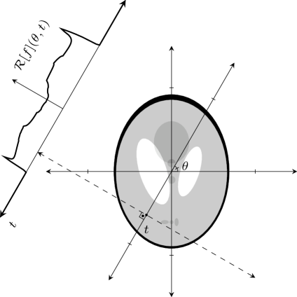
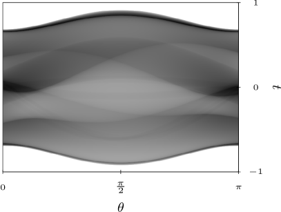
Figure 1: Left: integration path for the Radon transform. There, θ𝜃\theta is the angle between the normal to the integration path and the horizontal axis, and t𝑡t is the distance from the line of integration to the origin. Right: gray-scale image in the θ×t𝜃𝑡\theta\times t coordinate system of the Radon transform of the image shown on the left.

Before heading to the experimental details, we explain generalities of the tomographic image reconstruction problem. In tomography, the goal is to reconstruct an image ρ:2:𝜌superscript2\rho:\mathbb{R}^{2}\to\mathbb{R} from a finite number of approximate samples of its Radon transform [ρ]:[0,π)×:delimited-[]𝜌0𝜋\mathcal{R}[\rho]:[0,\pi)\times\mathbb{R}\to\mathbb{R}, which is defined as

[ρ](θ,t):=ρ(t(cosθsinθ)+s(sinθcosθ))ds,assigndelimited-[]𝜌𝜃𝑡superscriptsubscript𝜌𝑡binomial𝜃𝜃𝑠binomial𝜃𝜃differential-d𝑠\mathcal{R}\left[\rho\right](\theta,t):=\int_{-\infty}^{\infty}\rho\left(t\binom{\cos\theta}{\sin\theta}+s\binom{-\sin\theta}{\cos\theta}\right)\mathrm{d}s, (62)

see Figure 1 for an illustration. Assuming that the image belongs to a linear space spanned by a basis {ρ1,ρ2,,ρn}subscript𝜌1subscript𝜌2subscript𝜌𝑛\{\rho_{1},\rho_{2},\dots,\rho_{n}\} and because there is a finite number of samples bi[ρ](θi,ti)subscript𝑏𝑖delimited-[]𝜌subscript𝜃𝑖subscript𝑡𝑖b_{i}\approx\mathcal{R}\left[\rho\right](\theta_{i},t_{i}), i{1,2,,m}𝑖12𝑚i\in\{1,2,\dots,m\}, the problem is then reduced to a linear system of equations

R𝐱𝐛,𝑅𝐱𝐛R\mathbf{x}\approx\mathbf{b}, (63)

where the unknowns 𝐱n𝐱superscript𝑛\mathbf{x}\in\mathbb{R}^{n} are the coefficients of the linear combination that gives the reconstruction ρrecon:=j=1nxjρjassignsubscript𝜌reconsuperscriptsubscript𝑗1𝑛subscript𝑥𝑗subscript𝜌𝑗\rho_{\text{recon}}:=\sum_{j=1}^{n}x_{j}\rho_{j}. In practice the meaning of the approximation above has to be made clear, which can be done by, e.g., optimization. In this setting, the constrained least squares

𝐱argmin𝐲+nR𝐲𝐛2,𝐱subscriptargmin𝐲superscriptsubscript𝑛superscriptnorm𝑅𝐲𝐛2\mathbf{x}\in\operatorname*{arg\,min}_{\mathbf{y}\in\mathbb{R}_{+}^{n}}\|R\mathbf{y}-\mathbf{b}\|^{2}, (64)

is one among the many possible models. Because the tomographic reconstruction problem is poorly conditioned, regularization is commonly applied and the situation can in many cases be interpreted as the minimization of the sum of a smooth convex function f𝑓f and a non-smooth convex function ϕitalic-ϕ\phi as in (1), the problem which fast proximal gradient methods are designed to solve. In theory, because the Radon transform is a compact linear operator, its inverse is (moderately) ill-posed Engl et al. (2000). In practice, this ill-posedness can be problematic in some circumstances. For example, in acquisitions where the signal to noise ratio is below ideal such as when lower exposure to radiation is desired or when the source is less predictable such as in emission tomography. Beyond these cases, there might be reasons that make a shorter acquisition time necessary (for example, for 4D tomography), which might amplify the ill-posedness of the problem because higher scanning speeds are usually obtained by sampling radially at a lower rate.

5.1 Constrained Maximum Likelihood Tomography with Synchrotron Data

In synchrotron tomography, [ρ](θi,ti)delimited-[]𝜌subscript𝜃𝑖subscript𝑡𝑖\mathcal{R}\left[\rho\right](\theta_{i},t_{i}) can be estimated by a computation involving disubscript𝑑𝑖d_{i}, ωisubscript𝜔𝑖\omega_{i}, and pisubscript𝑝𝑖p_{i}, where

  • disubscript𝑑𝑖d_{i} is a measurement of the dark field, which is the expected number of detected events in the sensor during a scan without active source and without the object between source and detector;

  • ωisubscript𝜔𝑖\omega_{i} is a measurement of the flat field, which is the expected number of detected events in the sensor during a scan with active source and without the object between source and detector;

  • pisubscript𝑝𝑖p_{i} is the photon count, i.e., the number of events in the sensor during a scan with active source and with the object between source and detector.

Another idea is, instead of estimating [ρ](θi,ti)delimited-[]𝜌subscript𝜃𝑖subscript𝑡𝑖\mathcal{R}\left[\rho\right](\theta_{i},t_{i}) from dark field, flat field, and photon count data, to use the probabilistically inspired constrained model for transmission data from Erdoǧan and Fessler (1999), which we describe now. Let

f(𝐱)=i=1mhi((R𝐱)i),𝑓𝐱superscriptsubscript𝑖1𝑚subscript𝑖subscript𝑅𝐱𝑖f(\mathbf{x})=\sum_{i=1}^{m}h_{i}\left((R\mathbf{x})_{i}\right), (65)

where

hi(b)=ωieb+dipilog(ωieb+di).subscript𝑖𝑏subscript𝜔𝑖superscript𝑒𝑏subscript𝑑𝑖subscript𝑝𝑖subscript𝜔𝑖superscript𝑒𝑏subscript𝑑𝑖h_{i}(b)=\omega_{i}e^{-b}+d_{i}-p_{i}\log(\omega_{i}e^{-b}+d_{i}). (66)

Thus, the model consists of solving

min𝐱+nf(𝐱),subscript𝐱superscriptsubscript𝑛𝑓𝐱\min_{\mathbf{x}\in\mathbb{R}_{+}^{n}}\quad f(\mathbf{x}), (67)

which is equivalent to

min𝐱nf(𝐱)+ϕ(𝐱),subscript𝐱superscript𝑛𝑓𝐱italic-ϕ𝐱\min_{\mathbf{x}\in\mathbb{R}^{n}}\quad f(\mathbf{x})+\phi(\mathbf{x}), (68)

where ϕ(𝐱)=χ+n(𝐱)italic-ϕ𝐱subscript𝜒superscriptsubscript𝑛𝐱\phi(\mathbf{x})=\chi_{\mathbb{R}_{+}^{n}}(\mathbf{x}), with the indicator function χCsubscript𝜒𝐶\chi_{C} of a convex closed set C𝐶C defined as

χC(𝐱)={0if𝐱Cotherwise.subscript𝜒𝐶𝐱cases0if𝐱𝐶otherwise.\chi_{C}(\mathbf{x})=\begin{cases}0&\text{if}\quad\mathbf{x}\in C\\ \infty&\text{otherwise.}\end{cases} (69)

The proximal operator of the indicator function is the Euclidean projection:

proxχC(𝐱)=𝒫C(𝐱)=argmin𝐲C𝐱𝐲.subscriptproxsubscript𝜒𝐶𝐱subscript𝒫𝐶𝐱subscriptargmin𝐲𝐶norm𝐱𝐲\operatorname*{prox}_{\chi_{C}}(\mathbf{x})=\mathcal{P}_{C}(\mathbf{x})=\operatorname*{arg\,min}_{\mathbf{y}\in C}\|\mathbf{x}-\mathbf{y}\|. (70)

Data Geometry and Dimensions

Data was collected along mr=2048subscript𝑚𝑟2048m_{r}=2048 parallel lines on each one of the mv=512subscript𝑚𝑣512m_{v}=512 views and the path between emitter and detector for data point i𝑖i was parametrized by the pair (θi,ti)subscript𝜃𝑖subscript𝑡𝑖(\theta_{i},t_{i}) for i{1,2,,mrmv}𝑖12subscript𝑚𝑟subscript𝑚𝑣i\in\left\{1,2,\dots,m_{r}m_{v}\right\} in the following manner. First let us define κi{1,2,,mv}subscript𝜅𝑖12subscript𝑚𝑣\kappa_{i}\in\left\{1,2,\dots,m_{v}\right\} as κi:=1+(i1)/mrassignsubscript𝜅𝑖1𝑖1subscript𝑚𝑟\kappa_{i}:=1+\lfloor(i-1)/m_{r}\rfloor where x𝑥\lfloor x\rfloor is the largest integer smaller than or equal x𝑥x and i{1,2,,mr}subscript𝑖12subscript𝑚𝑟\ell_{i}\in\{1,2,\dots,m_{r}\} as i:=1+(i1)%mrassignsubscript𝑖1percent𝑖1subscript𝑚𝑟\ell_{i}:=1+(i-1)\%m_{r} where a%bpercent𝑎𝑏a\%b is the remainder of the integer division of a𝑎a\in\mathbb{N} by b𝑏b\in\mathbb{N}. Then, for i{1,2,,mrmv}𝑖12subscript𝑚𝑟subscript𝑚𝑣i\in\left\{1,2,\dots,m_{r}m_{v}\right\}, we have

θi=π(κi1)mv1andti=1+2(i1)mr1.formulae-sequencesubscript𝜃𝑖𝜋subscript𝜅𝑖1subscript𝑚𝑣1andsubscript𝑡𝑖12subscript𝑖1subscript𝑚𝑟1\theta_{i}=-\pi\frac{(\kappa_{i}-1)}{m_{v}-1}\quad\text{and}\quad t_{i}=-1+2\frac{(\ell_{i}-1)}{m_{r}-1}. (71)

The dimensions of the reconstructed images are n=20482𝑛superscript20482n=2048^{2}, that is, 2048×2048204820482048\times 2048 pixels.

Refer to caption
Refer to caption
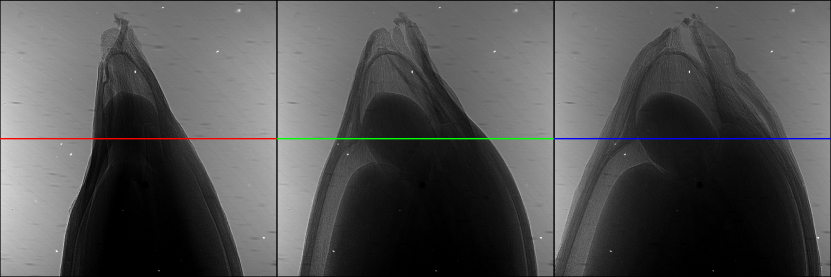
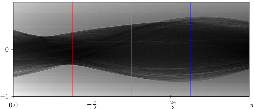
Figure 2: Top: three of the 512512512 images used in the reconstruction of a slice of an apple seed. These images depict the number of photons recorded on each sensor pixel, where brighter indicates more photons recorded. The solid lines indicate data corresponding to the slice that will be reconstructed in the experiments. Bottom: photon count data that will be used for the reconstruction of the slice. Each of the 512512512 rows of the data related to the same slice is used as a column in a representation of the data as samples of the photon counts in the θ×t𝜃𝑡\theta\times t plane. The color of each of the solid lines identifies the position where the corresponding data in the top row was used.

In the transmission tomography setup found at the Brazilian Synchrotron Light Laboratory, the object to be imaged is positioned between the synchrotron x-ray source and a scintillator that is digitally imaged by a CCD camera. Data from the κ𝜅\kappa-th readout from this camera provides a 2048×2048204820482048\times 2048 radio-graphic image that includes the photon counts at pixels of the camera corresponding to integration lines with parameters θ=π(κ1)/(mv1)𝜃𝜋𝜅1subscript𝑚𝑣1\theta=-\pi(\kappa-1)/\left(m_{v}-1\right) and t{1+2(1)mr1:{1,2,,mr}}𝑡conditional-set121subscript𝑚𝑟112subscript𝑚𝑟t\in\left\{-1+2\frac{(\ell-1)}{m_{r}-1}:\ell\in\left\{1,2,\dots,m_{r}\right\}\right\} not only for one two-dimensional slice, but simultaneously for 204820482048 parallel slices of the imaged volume. Reconstruction of each of the slices is later performed independently through the two-dimensional model. Figure 2 depicts the procedure used to obtain the photon count data pisubscript𝑝𝑖p_{i} that will be used for one slice reconstruction.

Algorithm 7 OISTA
1:  input L0>0subscript𝐿00L_{0}>0, β>1𝛽1\beta>1, 𝐱0nsubscript𝐱0superscript𝑛\mathbf{x}_{0}\in\mathbb{R}^{n}, N𝑁N\in\mathbb{N}
2:  set t1=1subscript𝑡11t_{1}=1, 𝐲1=𝐱0subscript𝐲1subscript𝐱0\mathbf{y}_{1}=\mathbf{x}_{0}
3:  for k=1,,N𝑘1𝑁k=1,...,N
4:      set Lk=Lk1subscript𝐿𝑘subscript𝐿𝑘1L_{k}=L_{k-1}
5:      while Ψ(PLk(𝐲k))>QLk(PLk(𝐲k),𝐲k)Ψsubscript𝑃subscript𝐿𝑘subscript𝐲𝑘subscript𝑄subscript𝐿𝑘subscript𝑃subscript𝐿𝑘subscript𝐲𝑘subscript𝐲𝑘\Psi\left(P_{L_{k}}(\mathbf{y}_{k})\right)>Q_{L_{k}}\left(P_{L_{k}}(\mathbf{y}_{k}),\mathbf{y}_{k}\right)
6:          set Lk=βLksubscript𝐿𝑘𝛽subscript𝐿𝑘L_{k}=\beta L_{k}
7:      set 𝐱k=PLk(𝐲k)subscript𝐱𝑘subscript𝑃subscript𝐿𝑘subscript𝐲𝑘\mathbf{x}_{k}=P_{L_{k}}(\mathbf{y}_{k})
8:      set tk+1=1+1+4tk22subscript𝑡𝑘1114superscriptsubscript𝑡𝑘22t_{k+1}=\frac{1+\sqrt{1+4t_{k}^{2}}}{2}
9:      set 𝐲k+1=𝐱k+tk1tk+1(𝐱k𝐱k1)+tktk+1(𝐱k𝐲k)subscript𝐲𝑘1subscript𝐱𝑘subscript𝑡𝑘1subscript𝑡𝑘1subscript𝐱𝑘subscript𝐱𝑘1subscript𝑡𝑘subscript𝑡𝑘1subscript𝐱𝑘subscript𝐲𝑘\mathbf{y}_{k+1}=\mathbf{x}_{k}+\frac{t_{k}-1}{t_{k+1}}\left(\mathbf{x}_{k}-\mathbf{x}_{k-1}\right)+\frac{t_{k}}{t_{k+1}}\left(\mathbf{x}_{k}-\mathbf{y}_{k}\right)

Algorithms

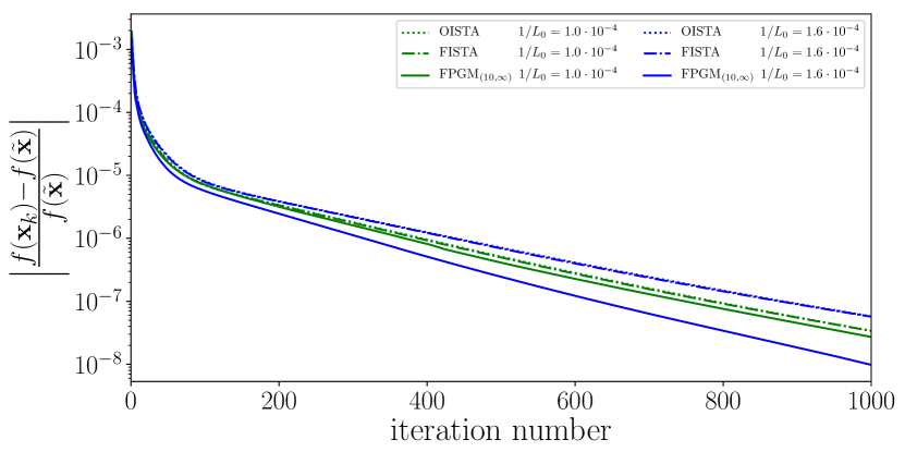
We have compared several algorithms regarding speed of reduction of objective function value. The methods experimented with are the following: FISTA (Algorithm 2) and OISTA (Algorithm 7), which we compare against FPGM (Algorithm 4). In every case, the starting image 𝐱0subscript𝐱0\mathbf{x}_{0} was set to an image such that all of its pixels have the same value and i=1m(R𝐱0)i=i=1mb~isuperscriptsubscript𝑖1𝑚subscript𝑅subscript𝐱0𝑖superscriptsubscript𝑖1𝑚subscript~𝑏𝑖\sum_{i=1}^{m}(R\mathbf{x}_{0})_{i}=\sum_{i=1}^{m}\tilde{b}_{i}, where b~isubscript~𝑏𝑖\tilde{b}_{i} are the estimates of the Radon Transform given by b~i=lnωidipidisubscript~𝑏𝑖subscript𝜔𝑖subscript𝑑𝑖subscript𝑝𝑖subscript𝑑𝑖\tilde{b}_{i}=\ln\frac{\omega_{i}-d_{i}}{p_{i}-d_{i}}. The parameter β𝛽\beta was set to 222 for all algorithms. This seemed a reasonable choice and we did not feel the need to experiment with this parameter. A first comparison uses K=10𝐾10K=10 and η¯=¯𝜂\overline{\eta}=\infty for FPGM and compares it to FISTA and OISTA. A second experiment considers only FPGM, but with three different set of parameters K𝐾K and η¯¯𝜂\overline{\eta}, namely (K,η¯){(10,),(10,2),(,)}𝐾¯𝜂10102(K,\overline{\eta})\in\{(10,\infty),(10,2),(\infty,\infty)\}. We denote the FPGM variations as FPGM(K,η¯)𝐾¯𝜂{}_{(K,\overline{\eta})} with (K,η¯){(10,),(10,2),(,)}𝐾¯𝜂10102(K,\overline{\eta})\in\{(10,\infty),(10,2),(\infty,\infty)\}. The reason why the value η¯=2¯𝜂2\overline{\eta}=2 was singled out among all the possible finite values for this parameter is that when ηk=2subscript𝜂𝑘2\eta_{k}=2 the FPGM iteration is identical to the one of OISTA, for which no convergence proof exists. This way we show that our theoretical results can explain why OISTA converges in some cases, while at the same time they give insights on when and why OISTA might not converge. Notice that the theoretical results presented above do not guarantee convergence of FPGM(∞,∞) because it may not satisfy (34). In fact, Figure 5 shows what seems to be an example of the algorithm not converging to an optimizer.

Computational Issues

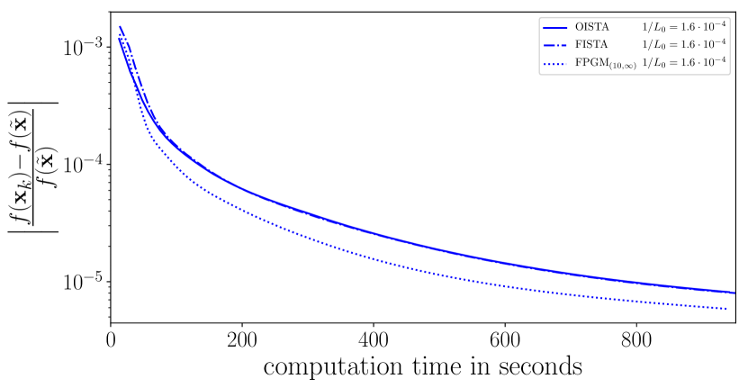
Because of the large data and image size, the matrix-vector products R𝐱𝑅𝐱R\mathbf{x} and RT𝐛superscript𝑅𝑇𝐛R^{T}\mathbf{b} were implemented in a parallel fashion and the computations were carried out by a Graphics Processing Unit (GPU) using C++ CUDA in order to obtain low running times for the reconstruction and thus to enable experimentation with a wide range of parameters and for a very large number of iterations. A Python wrapper for the GPU routines was used in order to implement all the other algorithm parts using the NumPy library. We have used the ray-tracing method from Han et al. (1999) for the on-the-fly computation of these matrix-vector products. All other computations were accomplished by the CPU. The computer had a GeForce Titan Xp GPU with 12GB of dedicated RAM and a Ryzen 5 2600 CPU with 16GB of available RAM. The algorithms are also practical when executed in less powerful hardware, as Figure 4 shows. In practice far less than 100010001000 iterations will be executed and the algorithm will be executed with a single set of parameters, which means that even modest CPUs such as the one used suffice for routine reconstruction. The single precision GPU implementation runs at around 121212 times faster than the double precision CPU implementation.
Refer to caption
Figure 3: Plot of objective function value at each iteration for two different starting step-size values in three different algorithms.
Refer to caption
Figure 4: Plot of objective function over time in three different algorithms, running on the CPU.

Discussion

We base our discussion on log-plots of the objective function reduction as iterations proceed. In these plots we represent the evolution of the relative difference between the object function value obtained by each algorithm and the value obtained by FISTA after 200020002000 iterations (using 1/L0=1.31041subscript𝐿01.3superscript104\nicefrac{{1}}{{L_{0}}}=1.3\cdot 10^{-4}). We denote the reference image obtained by this long run of FISTA by 𝐱~~𝐱\tilde{\mathbf{x}}. The starting stepsize for the long FISTA run was selected in order to obtain good convergence and running FISTA for twice as many iterations as the other methods ensured that the final iterations obtained this way by FISTA had better objective function value than the other methods.

For a comparison of FPGM with existing algorithms, we have tested the behavior of FPGM(10,∞) and compared it to FISTA and OISTA. We notice in Figure 3 that FPGM(10,∞) is very competitive regardless of the starting stepsize adopted within the experimented range. We have tried running the algorithm for a variety of stepsizes within the range 1/L0[9105,2104]1subscript𝐿09superscript1052superscript104\nicefrac{{1}}{{L_{0}}}\in[9\cdot 10^{-5},2\cdot 10^{-4}]. This range was chosen because it contains the value of 1/L10001subscript𝐿1000\nicefrac{{1}}{{L_{1000}}} obtained by the line search procedure if values above this range were used. This means that smaller stepsize values unnecessarily slow down the algorithms and should not be used, whereas for larger values the line search reduces the stepsize in the first few iterations to something within the adopted range. For the sake of legibility, we present the results obtained for only two values of 1/L01subscript𝐿0\nicefrac{{1}}{{L_{0}}} showing the typical behavior. We note that, for a favorable selection of starting stepsize FPGM outperforms noticeably the other methods, whereas for some values of the starting stepsize the improvements may be small.
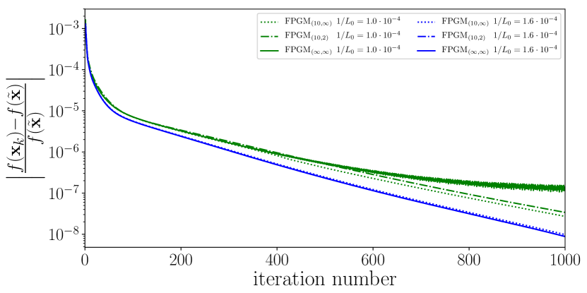
Refer to caption
Figure 5: Comparison of the behavior of the objective function value of the iterates of FPGM(K,η¯)𝐾¯𝜂{}_{(K,\overline{\eta})} for some values of parameters K𝐾K, η¯¯𝜂\overline{\eta}, and L0subscript𝐿0L_{0}. Notice that because FPGM(∞,∞) might not converge, oscillatory behavior is observed for some starting stepsize values.

Figure 5 illustrates an experiment designed to investigate sensitivity of Algorithm 4 to the choice of parameters K𝐾K and η¯¯𝜂\overline{\eta}. As it can be seen, at least for this combination of optimization model and data, FPGM(10,∞) and FPGM(10,2), which are provably convergent, appear to have advantages over FPGM(∞,∞), which does not necessarily satisfy (34) and, therefore, has no proven convergence. Also, it seems that limiting the value of ηksubscript𝜂𝑘\eta_{k} does not necessarily reduce convergence speed when all other parameters are the same. Convergent versions of FPGM did not present any drastic performance changes within the set of parameters used, which is a sign of robustness with relation to parameter selection.

5.2 Reconstruction from Simulated Data

In the present subsection we perform reconstruction from simulated data in order to be able to measure reconstruction quality. We have performed several similar experiments with the intention of performing statistical testing on the hypothesis that one algorithm performs better than the other with respect to a well defined mathematical figure of merit. We will first describe how each reconstruction experiment was performed and then we discuss the results of the statistical hypothesis testing.

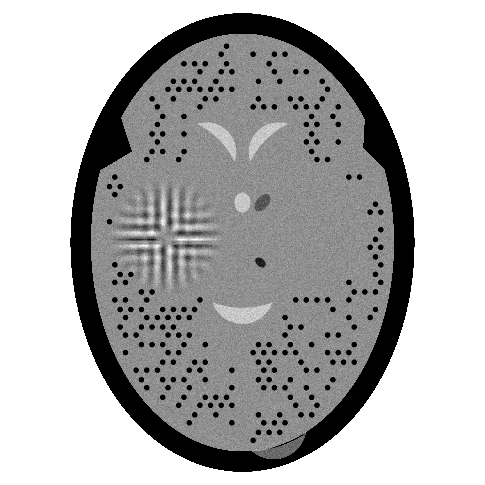
Refer to caption
Refer to caption
Figure 6: One of the possible phantoms used in the statistical hypothesis testing experiment. On the left, the full range of attenuation values of the phantom is shown, its minimum value represented as white and the maximum as black. On the right, values below 0.2040.2040.204 cm-1 are shown as white and values above 0.217650.217650.21765 cm-1 are shown as black.

Refer to captionRefer to captionRefer to caption

Figure 7: Left: First iteration of SupART to reach stopping criterion. Center: 50thsuperscript50th50^{\text{th}} iteration of FPGM5103(10,)superscriptsubscriptabsent105superscript103{}_{(10,\infty)}^{5\cdot 10^{-3}}. Right: 100thsuperscript100th100^{\text{th}} iteration of FPGM5103(10,)superscriptsubscriptabsent105superscript103{}_{(10,\infty)}^{5\cdot 10^{-3}}. Top: full images. Bottom: details for easier inspection.

Test Images and Projection Data

Each reconstruction experiment was based on a mathematical phantom defined from simple geometrical features, which can be seen in Figure 6. It has a skull-like high-attenuation feature around it, while possessing less contrasting objects inside the skull. Among the features inside the skull there are small similar circular objects scattered inside the inner structure. The number of such objects is constant, but its position vary on each experiment in the following form: each object must exist in a position or else to exist in the same position except that mirrored along the central vertical axis. The side where the circular object will be placed is selected at random with equal probability of selection for left and right placement. The other features of the phantom do not change from one experiment to another, except for a small random inhomogeneity, which may also be different from one experiment to another. Generation of the images, simulation of tomographic data from each generated image, and reconstruction from each of the simulated dataset was automatically handled by the "experimenter" feature of SNARK14 software.111SNARK14 may be downloaded free of charge from http://turing.iimas.unam.mx/SNARK14M/ For this set of experiments, the sequential implementations provided by SNARK14 were used instead of the specially crafted parallel algorithms used in the previous set of experiments.

For these experiments, data acquisition followed a divergent beam geometry where detectors are distributed in a circular strip centered at the X-ray source with source-to-origin distance (that is, the radius of the source’s circular path followed during acquisition) equal to 787878 cm and with source-to-detector distance (that is, the radius of the circular strip of detectors) equal to 110.735110.735110.735 cm. The simulated circular detector strip contained 693693693 detectors with the spacing between the center of successive detectors equal to 0.05330.05330.0533 cm. Each projection contains data from all 693693693 detectors and 180180180 of such projections were measured, 2superscript22^{\circ} apart from each other. Reconstructed images had 485×485485485485\times 485 pixels covering the square [9.1 cm,9.1 cm]2superscript9.1 cm9.1 cm2[-9.1\text{ cm},9.1\text{ cm}]^{2}.

Reconstruction Model

In these experiments, for the reconstruction with FPGM we used the least squares model with Total Variation regularization. Let us first define the Total Variation as

TV(𝐱):=i=1m(xixr(i))2+(xixa(i))2,assign𝑇𝑉𝐱superscriptsubscript𝑖1𝑚superscriptsubscript𝑥𝑖subscript𝑥𝑟𝑖2superscriptsubscript𝑥𝑖subscript𝑥𝑎𝑖2TV(\mathbf{x}):=\sum_{i=1}^{m}\sqrt{\left(x_{i}-x_{r(i)}\right)^{2}+\left(x_{i}-x_{a(i)}\right)^{2}}, (72)

where r(i)𝑟𝑖r(i) is the index of the pixel to the right of pixel i𝑖i and a(i)𝑎𝑖a(i) is the index of the pixel above pixel i𝑖i. The Total Variation regularization functional was chosen because of its computational convenience and good regularization properties for tomographic images.

Our model therefore is

min𝐱+nR𝐱𝐛2+λTV(𝐱),subscript𝐱superscriptsubscript𝑛superscriptnorm𝑅𝐱𝐛2𝜆𝑇𝑉𝐱\min_{\mathbf{x}\in\mathbb{R}_{+}^{n}}\quad\left\|R\mathbf{x}-\mathbf{b}\right\|^{2}+\lambda TV(\mathbf{x}), (73)

where Rm×n𝑅superscript𝑚𝑛R\in\mathbb{R}^{m\times n} is the matrix representing the discretization of the Radon Transform and 𝐛n𝐛superscript𝑛\mathbf{b}\in\mathbb{R}^{n} contains the simulated data. This model can be rewritten as

min𝐱nf(𝐱)+ϕ(𝐱),subscript𝐱superscript𝑛𝑓𝐱italic-ϕ𝐱\min_{\mathbf{x}\in\mathbb{R}^{n}}\quad f(\mathbf{x})+\phi(\mathbf{x}), (74)

where f(𝐱)=R𝐱𝐛2𝑓𝐱superscriptnorm𝑅𝐱𝐛2f(\mathbf{x})=\left\|R\mathbf{x}-\mathbf{b}\right\|^{2} and ϕ(𝐱)=λTV(𝐱)+χ+n(𝐱)italic-ϕ𝐱𝜆𝑇𝑉𝐱subscript𝜒superscriptsubscript𝑛𝐱\phi(\mathbf{x})=\lambda TV(\mathbf{x})+\chi_{\mathbb{R}_{+}^{n}}(\mathbf{x}). The proximal operator for ϕ(𝐱)=λTV(𝐱)+χ+n(𝐱)italic-ϕ𝐱𝜆𝑇𝑉𝐱subscript𝜒superscriptsubscript𝑛𝐱\phi(\mathbf{x})=\lambda TV(\mathbf{x})+\chi_{\mathbb{R}_{+}^{n}}(\mathbf{x}) was approximately computed by 101010 steps of the fast gradient method for the dual formulation of the constrained TV𝑇𝑉TV proximal problem, according to Beck and Teboulle (2009b).

ART

One of the tested algorithms is FPGM(10,∞), as described above. The other is a superiorized version of the Algebraic Reconstruction Technique (ART). ART is a common denomination for a series of algorithms that sequentially update the reconstructed image using one row of the system R𝐱=𝐛𝑅𝐱𝐛R\mathbf{x}=\mathbf{b} (where 𝐛𝐛\mathbf{b} is the tomographic data and R𝑅R is the projection matrix) at a time. The meaning of "superiorized" will be explained after we describe ART itself. The precise version of ART used here is described as Algorithm 8 below, where 𝐫isubscript𝐫𝑖\mathbf{r}_{i} is the i𝑖i-th row of the matrix R𝑅R (an n𝑛n-dimensional row-vector).

Algorithm 8 ART
1:  input α𝛼\alpha\in\mathbb{R}, {i0,i1,,im1}subscript𝑖0subscript𝑖1subscript𝑖𝑚1\left\{i_{0},i_{1},\dots,i_{m-1}\right\}\subset\mathbb{N}, 𝐱n𝐱superscript𝑛\mathbf{x}\in\mathbb{R}^{n}, 𝐛m𝐛superscript𝑚\mathbf{b}\in\mathbb{R}^{m}
2:  set 𝐲0=𝐱subscript𝐲0𝐱\mathrm{\mathbf{y}_{0}}=\mathbf{x}
3:  for =0,,m10𝑚1\ell=0,...,m-1
4:      set 𝐲+1=𝐲α𝐫iT,𝐲𝐛i𝐫iT2𝐫iTsubscript𝐲1subscript𝐲𝛼superscriptsubscript𝐫subscript𝑖𝑇subscript𝐲subscript𝐛subscript𝑖superscriptnormsuperscriptsubscript𝐫subscript𝑖𝑇2superscriptsubscript𝐫subscript𝑖𝑇\mathbf{y}_{\ell+1}=\mathbf{y}_{\ell}-\alpha\frac{\left\langle\mathbf{r}_{i_{\ell}}^{T},\mathbf{y}_{\ell}\right\rangle-\mathbf{b}_{i_{\ell}}}{\left\|\mathbf{r}_{i_{\ell}}^{T}\right\|^{2}}\mathbf{r}_{i_{\ell}}^{T}
5:  return 𝐲msubscript𝐲𝑚\mathbf{y}_{m}

We will denote the result of the application of Algorithm 8 to a given 𝐱n𝐱superscript𝑛\mathbf{x}\in\mathbb{R}^{n} as ART(𝐱)𝐱(\mathbf{x}), omitting the other input parameters that will be kept fixed as follows: α=0.05𝛼0.05\alpha=0.05, which is known as the relaxation parameter, 𝐛m𝐛superscript𝑚\mathbf{b}\in\mathbb{R}^{m} which is the tomographic data, and the sequence {i0,i1,,im1}subscript𝑖0subscript𝑖1subscript𝑖𝑚1\left\{i_{0},i_{1},\dots,i_{m-1}\right\}, that determines the order of processing of the tomographic data within the full cycle of Algorithm 8, which is defined according to the "efficient" sequence described in Herman and Meyer (1993). This sequence was shown experimentally to improve convergence of the method.

Superiorization

Superiorization is a technique for the modification of iterative optimization (or feasibility) algorithms that possess resiliency to summable perturbations. It consists of replacing the iteration 𝐱ksubscript𝐱𝑘\mathbf{x}_{k} of a given algorithm by a perturbed version 𝐱~ksubscript~𝐱𝑘\tilde{\mathbf{x}}_{k} prior to applying the computations that will lead to the next iteration 𝐱k+1subscript𝐱𝑘1\mathbf{x}_{k+1} of the method. The perturbations, which we may denote as 𝐬k:=𝐱~k𝐱kassignsubscript𝐬𝑘subscript~𝐱𝑘subscript𝐱𝑘\mathbf{s}_{k}:=\tilde{\mathbf{x}}_{k}-\mathbf{x}_{k}, are usually designed to improve the iterates according to a secondary criterion represented by a function ϕ:n:italic-ϕsuperscript𝑛\phi:\mathbb{R}^{n}\to\mathbb{R}. By an improvement we mean a reduction of the value of ϕitalic-ϕ\phi, that is, 𝐬ksubscript𝐬𝑘\mathbf{s}_{k} is normally designed so that ϕ(𝐱k+𝐬k)ϕ(𝐱k)italic-ϕsubscript𝐱𝑘subscript𝐬𝑘italic-ϕsubscript𝐱𝑘\phi\left(\mathbf{x}_{k}+\mathbf{s}_{k}\right)\leq\phi\left(\mathbf{x}_{k}\right). In our experiments we have used ϕ=TVitalic-ϕ𝑇𝑉\phi=TV, i.e., the Total Variation defined in (72) is the secondary criterion for superiorization.

Algorithm 9 describes the procedure that we use to superiorize ART in our experiments. It makes use of the concept of non-ascending vectors. We define the set ~ϕ(𝐱)~italic-ϕ𝐱\tilde{\partial}\phi(\mathbf{x}) of non-ascending vectors for a convex function ϕ:n:italic-ϕsuperscript𝑛\phi:\mathbb{R}^{n}\to\mathbb{R} from a point 𝐱n𝐱superscript𝑛\mathbf{x}\in\mathbb{R}^{n} as the set of vectors 𝐭n𝐭superscript𝑛\mathbf{t}\in\mathbb{R}^{n} with 𝐭1norm𝐭1\|\mathbf{t}\|\leq 1 and such that there is B>0𝐵0B>0 for which b[0,B]𝑏0𝐵b\in[0,B] implies that ϕ(𝐱+b𝐭)ϕ(𝐱)italic-ϕ𝐱𝑏𝐭italic-ϕ𝐱\phi(\mathbf{x}+b\mathbf{t})\leq\phi(\mathbf{x}). Notice that 𝟎~ϕ(𝐱)0~italic-ϕ𝐱\mathbf{0}\in\tilde{\partial}\phi(\mathbf{x}), meaning that the set of non-ascending vectors is never empty. Following (Herman et al., 2012, Theorem 2), we can construct a non-ascending vector 𝐭𝐭\mathbf{t} for ϕitalic-ϕ\phi from 𝐱𝐱\mathbf{x} as follows, first componentwise defining an auxiliary vector 𝐭~n~𝐭superscript𝑛\tilde{\mathbf{t}}\in\mathbb{R}^{n} as

t~i={ϕxi(𝐱)if ϕxi(𝐱) is well defined0otherwise,and then defining 𝐭={𝐭~𝐭~if 𝐭~𝟎𝟎otherwise.formulae-sequencesubscript~𝑡𝑖casesitalic-ϕsubscript𝑥𝑖𝐱if italic-ϕsubscript𝑥𝑖𝐱 is well defined0otherwise,and then defining 𝐭cases~𝐭norm~𝐭if ~𝐭00otherwise.\tilde{t}_{i}=\begin{cases}\frac{\partial\phi}{\partial x_{i}}(\mathbf{x})&\text{if }\frac{\partial\phi}{\partial x_{i}}(\mathbf{x})\text{ is well defined}\\ 0&\text{otherwise,}\end{cases}\quad\text{and then defining\quad$\mathbf{t}$}=\begin{cases}-\frac{\tilde{\mathbf{t}}}{\|\tilde{\mathbf{t}}\|}&\text{if }\tilde{\mathbf{t}}\neq\mathbf{0}\\ \mathbf{0}&\text{otherwise.}\end{cases} (75)

We will denote the output of Algorithm 9 for given 𝐱n𝐱superscript𝑛\mathbf{x}\in\mathbb{R}^{n} and l𝑙l\in\mathbb{N} as SupTV(𝐱,l)𝐱𝑙(\mathbf{x},l), omitting parameters a𝑎a, b𝑏b and I𝐼I, which were kept fixed with the values a=1104𝑎1superscript104a=1-10^{-4}, b=3102𝑏3superscript102b=3\cdot 10^{-2}, and I=10𝐼10I=10.

Algorithm 9 SupTV
1:  input 𝐱n𝐱superscript𝑛\mathbf{x}\in\mathbb{R}^{n}, l𝑙l\in\mathbb{N}, a(0,1)𝑎01a\in(0,1), b(0,),𝑏0b\in(0,\infty), I𝐼I\in\mathbb{N}
2:  set 𝐲=𝐱𝐲𝐱\mathbf{y}=\mathbf{x}
3:  for i=1,2,,I𝑖12𝐼i=1,2,\dots,I
4:     set 𝐭~TV(𝐲)𝐭~𝑇𝑉𝐲\mathbf{t}\in\tilde{\partial}TV(\mathbf{y})
5:     do
6:        set b~=bal~𝑏𝑏superscript𝑎𝑙\tilde{b}=ba^{l}
7:        set 𝐲~=𝐲+b~𝐭~𝐲𝐲~𝑏𝐭\tilde{\mathbf{y}}=\mathbf{y}+\tilde{b}\mathbf{t}
8:        set l=l+1𝑙𝑙1l=l+1
9:     while TV(𝐲~)>TV(𝐲)𝑇𝑉~𝐲𝑇𝑉𝐲TV(\tilde{\mathbf{y}})>TV(\mathbf{y})
10:     set 𝐲=𝐲~𝐲~𝐲\mathbf{y}=\tilde{\mathbf{y}}
11:  return (𝐲,l)𝐲𝑙(\mathbf{y},l)

It is important to notice that superiorization according to the criterion ϕitalic-ϕ\phi does not mean minimization of that criterion. This makes the approach much more flexible than optimization because the theory is easier to develop for a large variety of secondary criteria. On the other hand, it is clear that, because there is no guarantee of minimization, there may exist images that are equally data-consistent than those obtained by superiorization, but that are better according to ϕitalic-ϕ\phi. In practice, however, superiorized methods have been shown to be almost as fast as the non-superiorized version of the same method, to be very flexible and simple to use in practice, and to deliver considerably improved results when compared to its non-superiorized counterpart.

Algorithm 10 SupART
1:  input 𝐱0nsubscript𝐱0superscript𝑛\mathbf{x}_{0}\in\mathbb{R}^{n}, ϵitalic-ϵ\epsilon\in\mathbb{R}, 𝐛m𝐛superscript𝑚\mathbf{b}\in\mathbb{R}^{m}
2:  set l0=0subscript𝑙00l_{0}=0, k=0𝑘0k=0
3:  while R𝐱k𝐛2>ϵsuperscriptnorm𝑅subscript𝐱𝑘𝐛2italic-ϵ\left\|R\mathbf{x}_{k}-\mathbf{b}\right\|^{2}>\epsilon
4:     set (𝐱k+1/2,lk+1)=SupTV(𝐱k,lk)subscript𝐱𝑘12subscript𝑙𝑘1SupTVsubscript𝐱𝑘subscript𝑙𝑘\left(\mathbf{x}_{k+\nicefrac{{1}}{{2}}},l_{k+1}\right)=\text{SupTV}\left(\mathbb{\mathbf{x}}_{k},l_{k}\right)
5:     set 𝐱k+1=ART(𝐱k+1/2)subscript𝐱𝑘1ARTsubscript𝐱𝑘12\mathbf{x}_{k+1}=\text{ART}\left(\mathbb{\mathbf{x}}_{k+\nicefrac{{1}}{{2}}}\right)
6:     set k=k+1𝑘𝑘1k=k+1
7:  return 𝐱ksubscript𝐱𝑘\mathbf{x}_{k}

SupART

We can finally precisely define the algorithm that we have compared to FPGM in the experiments described in the present subsection. Each iteration of Superiorized ART (SupART), presented in Algorithm 10, is defined as application of Algorithm 9 followed by application of Algorithm 8. Unlike FPGM which uses a prescribed number of iterations, our version of SupART uses a stopping criterion based in data-fidelity, as measured by the squared residual R𝐱𝐛2superscriptnorm𝑅𝐱𝐛2\|R\mathbf{x}-\mathbf{b}\|^{2}. We have done so in order to force the images obtained by SupART to have a data-fidelity value that is similar to those obtained by FPGM. We will describe precisely how it was done below, when discussing the parameter selection for the algorithms and models.

Parameter Selection

Algorithm FPGM(10,∞) was used with parameters L0=1subscript𝐿01L_{0}=1, β=2𝛽2\beta=2, and N=100𝑁100N=100 in order to solve model (73). In this case we are not comparing convergence speed between variations of the same algorithm, so the choice of parameters is not critical and these values work well in practice. For the model to be fully defined, the value of regularization parameter λ𝜆\lambda has to be specified. We now describe how we have decided which values to use for λ𝜆\lambda: We have generated a phantom and simulated tomographic data from this phantom as described above, and then ran the method for the set of parameters λ{104,5104,103,5103,102,5102}𝜆superscript1045superscript104superscript1035superscript103superscript1025superscript102\lambda\in\{10^{-4},5\cdot 10^{-4},10^{-3},5\cdot 10^{-3},10^{-2},5\cdot 10^{-2}\}. We verified that, among these, the value λ=5103𝜆5superscript103\lambda=5\cdot 10^{-3} provided the highest value of the Imagewise Region of Interest (IROI) figure of merit (the IROI is precisely described below, see (76)). Then, we have selected two other values for the regularization parameter within the same order of magnitude, leading to the final set of regularization parameters that were used in the final algorithmic comparison: λ{4,5,6}103𝜆456superscript103\lambda\in\{4,5,6\}\cdot 10^{-3}.

SupART has already been tested for this reconstruction problem in Garduño and Herman (2017), and we have used the (already mentioned above) same set of parameters as in that reference (α=0.05𝛼0.05\alpha=0.05, a=1104𝑎1superscript104a=1-10^{-4}, b=3102𝑏3superscript102b=3\cdot 10^{-2}) with one exception. In Garduño and Herman (2017) the authors have used I=40𝐼40I=40, while we have used I=10𝐼10I=10 in order to match the number of the iterations used by the approximation algorithm for the proximal operator of the TV𝑇𝑉TV that is used in FPGM. SupART also requires the determination of the stopping parameter ϵitalic-ϵ\epsilon, which we have selected to be 2.332.332.33 because this is, up to three digits accuracy, what FPGM(10,∞) obtained after 100100100 iterations when solving (73) with λ=5103𝜆5superscript103\lambda=5\cdot 10^{-3}.

Finally, both FPGM and SupART require the selection of a starting image 𝐱0subscript𝐱0\mathbf{x}_{0}, which we have selected to be a uniform image such that i=1m(R𝐱0)i=i=1mbisuperscriptsubscript𝑖1𝑚subscript𝑅subscript𝐱0𝑖superscriptsubscript𝑖1𝑚subscript𝑏𝑖\sum_{i=1}^{m}\left(R\mathbf{x}_{0}\right)_{i}=\sum_{i=1}^{m}b_{i}.

Image Reconstruction Evaluation

Comparison of the tested algorithms was done according to the IROI figure of merit. The IROI is defined in Narayan and Herman (1999) and we provide a succinct explanation of it here. The IROI considers only paired structures, which in our case were each of the small circles (tumors) in the phantom shown at Figure 6 and its empty counterpart on the other side of the phantom. We associate each of these pairs of structures with an index ranging from 111 to S𝑆S. Let, for s{1,2,,S}𝑠12𝑆s\in\{1,2,\dots,S\}, αtp(s)superscriptsubscript𝛼𝑡𝑝𝑠\alpha_{t}^{p}(s) be the average density in the phantom on the region where the tumor s𝑠s is present, and αnp(s)superscriptsubscript𝛼𝑛𝑝𝑠\alpha_{n}^{p}(s) be the average density in the phantom on the respective region where the tumor s𝑠s is not present. Similarly, αtr(s)superscriptsubscript𝛼𝑡𝑟𝑠\alpha_{t}^{r}(s) and αnr(s)superscriptsubscript𝛼𝑛𝑟𝑠\alpha_{n}^{r}(s) are the average values of these regions in the reconstructed images. Then, the value of the IROI is given by

s=1S(αtr(s)αnr(s))s=1S(αnr(s)1Ss=1Sαnr(s))2/s=1S(αtp(s)αnp(s))s=1S(αnp(s)1Ss=1Sαnp(s))2.superscriptsubscript𝑠1𝑆superscriptsubscript𝛼𝑡𝑟𝑠superscriptsubscript𝛼𝑛𝑟𝑠superscriptsubscript𝑠1𝑆superscriptsuperscriptsubscript𝛼𝑛𝑟𝑠1𝑆superscriptsubscriptsuperscript𝑠1𝑆superscriptsubscript𝛼𝑛𝑟superscript𝑠2superscriptsubscript𝑠1𝑆superscriptsubscript𝛼𝑡𝑝𝑠superscriptsubscript𝛼𝑛𝑝𝑠superscriptsubscript𝑠1𝑆superscriptsuperscriptsubscript𝛼𝑛𝑝𝑠1𝑆superscriptsubscriptsuperscript𝑠1𝑆superscriptsubscript𝛼𝑛𝑝superscript𝑠2\frac{\sum_{s=1}^{S}\bigl{(}\alpha_{t}^{r}(s)-\alpha_{n}^{r}(s)\bigr{)}}{\sum_{s=1}^{S}\left(\alpha_{n}^{r}(s)-\frac{1}{S}\sum_{s^{\prime}=1}^{S}\alpha_{n}^{r}(s^{\prime})\right)^{2}}/\frac{\sum_{s=1}^{S}\bigl{(}\alpha_{t}^{p}(s)-\alpha_{n}^{p}(s)\bigr{)}}{\sum_{s=1}^{S}\left(\alpha_{n}^{p}(s)-\frac{1}{S}\sum_{s^{\prime}=1}^{S}\alpha_{n}^{p}(s^{\prime})\right)^{2}}. (76)

Large IROI values mean that we have large differences αtr(s)αnr(s)superscriptsubscript𝛼𝑡𝑟𝑠superscriptsubscript𝛼𝑛𝑟𝑠\alpha_{t}^{r}(s)-\alpha_{n}^{r}(s) and, therefore, that reconstructed images with large IROI values tend to offer easier detectability of the tumors in the regions of interest than images with low IROI.

The last sentence indicates the essential nature of IROI; its purpose is to measure the efficacy of an algorithm for tumor detectability in the reconstructions. It is different from measures based on the overall similarity between the phantoms and their reconstructions, such as structural similarity (SSIM). Those other measures are likely to indicate better the perceived quality of the whole reconstruction, but IROI is more useful for evaluating the diagnostic efficacy of a reconstruction algorithm for the specific task of tumor detection Narayan and Herman (1999).

Discussion

We have performed 303030 repetitions of the cycle of (i) generating a random phantom, (ii) simulating projection data from the phantom, (iii) reconstructing images from the simulated data with SupART and FPGM (for the three versions of model (73) with λ{4,5,6}103𝜆456superscript103\lambda\in\{4,5,6\}\cdot 10^{-3}), and (iv) computing the IROI of the reconstructed images. These 303030 repetitions were used for statistical testing of the null hypothesis (H0) "SupART reconstructs an image with IROI equally large as the one obtained by FPGMλ(10,)superscriptsubscriptabsent10𝜆{}_{(10,\infty)}^{\lambda}", where FPGMλ(10,)superscriptsubscriptabsent10𝜆{}_{(10,\infty)}^{\lambda} denotes FPGM(10,∞) applied to the solution of (73) with regularization parameter λ𝜆\lambda. The results can be seen on Table 1, where we have denoted the estimated likelihood of rejecting H0 while it is true by P0subscript𝑃0P_{0}.

Figure 7 shows reconstructions obtained by SupART and FPGM5103(10,)superscriptsubscriptabsent105superscript103{}_{(10,\infty)}^{5\cdot 10^{-3}} in the last of the 303030 experiments for an illustration of the difference of the results of the algorithms. We remark that although FPGM is a fast algorithm, certain features take a large number of iterations to be accurately captured by the method. Notice how a low-frequency low-contrast artifact in the form of radial waves can be seen in the 50thsuperscript50th50^{\text{th}} iteration of FPGM(10,∞). This artifact is not present if the algorithm is allowed to run for more time. This is not a feature exclusively present in FPGM nor it is exclusive to the particular selection of algorithmic parameters that were used in our experiments, but rather a common issue with all the fast proximal gradient methods which might not have been noticed before because low-contrast features such as those in the phantom we use are not usually investigated in simulated reconstructions. Indeed, even Conjugate Gradient methods seem to present such kind of artifact (see, e.g., Figure 4(b) in Zibetti et al. (2018)).

Although it can be seen that in this particular setting the FPGM reconstructions are consistently better than SupART reconstructions, we make no claims that FPGM performs better than SupART in general because the experiments were performed for a particular set of simulation and algorithmic parameters. It was not our intent to optimize SupART’s parameter for this specific reconstruction problem, but it may well be the case that SupART could obtain results as good (or better) as those obtained by FPGM if the parameters were more carefully adjusted for the particular problem at hand. However, the experiments allow us to conclude that FPGM is competitive with state-of-the-art methods in terms of image quality reconstruction.

Algorithm Mean IROI P0subscript𝑃0P_{0}
FPGM4103(10,)superscriptsubscriptabsent104superscript103{}_{(10,\infty)}^{4\cdot 10^{-3}} 0.19140.19140.1914 3.0931083.093superscript1083.093\cdot 10^{-8}
FPGM5103(10,)superscriptsubscriptabsent105superscript103{}_{(10,\infty)}^{5\cdot 10^{-3}} 0.18830.18830.1883 3.4371083.437superscript1083.437\cdot 10^{-8}
FPGM6103(10,)superscriptsubscriptabsent106superscript103{}_{(10,\infty)}^{6\cdot 10^{-3}} 0.16230.16230.1623 1.3421071.342superscript1071.342\cdot 10^{-7}
SupART 0.14380.14380.1438 N/A
Table 1: Mean IROIs (larger is better) and estimated probabilities of rejecting a true null hypothesis.

6 Conclusions and Future Work

We have introduced a new algorithm called FPGM with convergence rate O(1/k2)𝑂1superscript𝑘2O(1/k^{2}) for the minimization of a separable smooth plus nonsmooth convex function. The convergence theory we have developed for this algorithm explains why OISTA Kim and Fessler (2016) converges in many circumstances even though in the worst-case scenario OISTA is non-convergent Taylor et al. (2017). In large-scale experiments with real world data, FPGM consistently outperforms, from the viewpoint of objective function reduction, FISTA, and in many cases FPGM performs better than OISTA in practice. Experiments performed from simulated data showed that FPGM presents reconstructed images of good quality, but it was noticed that a large number of iterations may be required in order to eliminate low-contrast artifacts that are present in the early iterations of the algorithm. In future research on this subject we plan to investigate the causes of such artifacts and to devise ways of avoiding them occurring in the early iterates Aharon et al. (2006).

Acknowledgments

This study has support by NIH grants R01-AR060238, R01-AR067156, and R01-AR068966, and was performed under the rubric of the Center of Advanced Imaging Innovation and Research (CAI2R), a NIBIB Biomedical Technology Resource Center (NIH P41-EB017183). E. S. Helou was partially supported by FAPESP grants 2013/07375-0 and 2016/24286-9, and CNPq grant 310893/2019-4. We are also indebted to LNLS for the beam time granted through proposal number 20160215 and to NVIDIA for the GPU used in the experiments, which was obtained through the NVIDIA Higher Education and Research Grants.

References

  • Aharon et al. (2006) Aharon M, Elad M, Bruckstein A (2006) K-SVD: An algorithm for designing overcomplete dictionaries for sparse representation. IEEE Transactions on Signal Processing 54(11):4311–4322, DOI 10.1109/TSP.2006.881199, 59749104367
  • Beck and Teboulle (2009a) Beck A, Teboulle M (2009a) A fast iterative shrinkage-thresholding algorithm for linear inverse problems. SIAM Journal on Imaging Sciences 2(1):183–202, DOI 10.1137/080716542
  • Beck and Teboulle (2009b) Beck A, Teboulle M (2009b) Fast gradient-based algorithms for constrained total variation image denoising and deblurring problems. IEEE Transactions on Image Processing 18(11):2419–2434, DOI 10.1109/TIP.2009.2028250
  • Bioucas-Dias and Figueiredo (2007) Bioucas-Dias JM, Figueiredo MAT (2007) A new TwIST: Two-step iterative shrinkage/thresholding algorithms for image restoration. IEEE Transactions on Image Processing 16(12):29923004, DOI 10.1109/TIP.2007.909319
  • Donoho (2006) Donoho DL (2006) Compressed sensing. IEEE Transactions on Information Theory 52(4):1289–1306, DOI 10.1109/TIT.2006.871582, URL http://ieeexplore.ieee.org/xpl/freeabs_all.jsp?isnumber=33885&arnumber=1614066&count=44&index=0
  • Drori and Teboulle (2014) Drori Y, Teboulle M (2014) Performance of first-order methods for smooth convex minimization: a novel approach. Mathematical Programming 145(1–2):451–482, DOI 10.1007/s00365-007-9003-x
  • Engl et al. (2000) Engl HW, Hanke M, Neubauer A (2000) Regularization of Inverse Problems. Kluwer Academic Publishers
  • Erdoǧan and Fessler (1999) Erdoǧan H, Fessler JA (1999) Ordered subsets algorithms for transmission tomography. Physics in Medicine and Biology 44(11):2835–2851, DOI http://dx.doi.org/10.1088/0031-9155/44/11/311
  • Garduño and Herman (2017) Garduño E, Herman GT (2017) Computerized tomography with total variation and with shearlets. Inverse Problems 33(4):44011–44024, DOI 10.1088/1361-6420/33/4/044011
  • Gong et al. (2013) Gong P, Zhang C, Lu Z, Huang JZ, Ye J (2013) A general iterative shrinkage and thresholding algorithm for non-convex regularized optimization problems. In: Proceedings of the 30th International Conference on Machine Learning, vol 28, pp 37–45, URL https://dl.acm.org/doi/abs/10.5555/3042817.3042898
  • Grippo et al. (1986) Grippo L, Lampariello F, Lucidi S (1986) A nonmonotone line search technique for Newton’s method. SIAM Journal on Numerical Analysis 23(4):707–716, DOI 10.1137/0723046, URL http://epubs.siam.org/doi/abs/10.1137/0723046
  • Han et al. (1999) Han G, Liang Z, You J (1999) A fast ray-tracing technique for TCT and ECT studies. In: IEEE Nuclear Science Symposium Conference Record, IEEE, 3, pp 1515–1518, DOI 10.1109/NSSMIC.1999.842846, URL http://ieeexplore.ieee.org/xpls/abs_all.jsp?arnumber=842846&tag=1
  • Herman (2009) Herman GT (2009) Fundamentals of Computerized Tomography: Image Reconstruction from Projections, 2nd edn. Springer-Verlag, London
  • Herman and Meyer (1993) Herman GT, Meyer LB (1993) Algebraic reconstruction techniques can be made computationally efficient. IEEE Transactions on Medical Imaging 12(3):600–609, DOI 10.1109/42.241889, URL http://ieeexplore.ieee.org/xpl/freeabs_all.jsp?isnumber=6214&arnumber=241889&count=27&index=24
  • Herman et al. (2012) Herman GT, Garduño E, Davidi R, Censor Y (2012) Superiorization: An optimization heuristic for medical physics. Medical Physics 39(9):5532–5546, DOI 10.1118/1.4745566
  • Hiriart-Urruty and Lemaréchal (1993) Hiriart-Urruty JB, Lemaréchal C (1993) Convex Analysis and Minimization Algorithms. Springer-Verlag, Berlin
  • Kim and Fessler (2015) Kim D, Fessler JA (2015) An optimized first-order method for image restoration. In: IEEE International Conference on Image Processing, IEEE, pp 3675–3679, DOI 10.1109/ICIP.2015.7351490
  • Kim and Fessler (2016) Kim D, Fessler JA (2016) Optimized first-order methods for smooth convex minimization. Mathematical Programming 159(1-2):81–107, DOI 10.1007/s10107-015-0949-3, 1406.5468
  • Narayan and Herman (1999) Narayan TK, Herman GT (1999) Prediction of human observer performance by numerical observers: An experimental study. Journal of the Optical Society of America A 16(3):679–693, DOI 10.1364/JOSAA.16.000679
  • Nesterov (1983) Nesterov YE (1983) A method for solving a convex programming problem with convergence rate O(1/k2)𝑂1superscript𝑘2O(1/k^{2}). Soviet Mathematics Doklady 27(3):372–376
  • Nesterov (2004) Nesterov YE (2004) Introductory Lectures on Convex Optimization: A Basic Course. Springer, New York
  • Parikh and Boyd (2014) Parikh N, Boyd S (2014) Proximal algorithms. Foundations and Trends in Optimization 1(3):127–239, DOI 10.1561/2400000003
  • Taylor et al. (2017) Taylor AB, Hendrickx JM, cois Glineur F (2017) Exact worst-case performance of first-order methods for composite convex optimization. SIAM Journal on Optimization 27(3):1283–1313, DOI 10.1137/16M108104X
  • Wright et al. (2009) Wright SJ, Nowak RD, Figueiredo MAT (2009) Sparse reconstruction by separable approximation. IEEE Transactions on Signal Processing 57(7):2479–2493, DOI 10.1109/TSP.2009.2016892
  • Yamagishi and Yamada (2011) Yamagishi M, Yamada I (2011) Over-relaxation of the fast iterative shrinkage-thresholding algorithm with variable stepsize. Inverse Problems 27(10):105008, DOI 10.1088/0266-5611/27/10/105008
  • Zhang and Hager (2004) Zhang H, Hager WW (2004) A nonmonotone line search technique and its application to unconstrained optimization. SIAM Journal on Optimization 14(4):1043–1056, DOI 10.1137/S1052623403428208
  • Zibetti et al. (2018) Zibetti MVW, Lin C, Herman GT (2018) Total variation superiorized conjugate gradient method for image reconstruction. Inverse Problems 34(3):34001–340026, DOI 10.1088/1361-6420/aaa49b
  • Zibetti et al. (2019) Zibetti MVW, Helou ES, Regatte RR, Herman GT (2019) Monotone FISTA With Variable Acceleration for Compressed Sensing Magnetic Resonance Imaging. IEEE Transactions on Computational Imaging 5(1):109–119, DOI 10.1109/TCI.2018.2882681