Fast Transit Computation Using Tabulated Stellar Intensities

Abstract

Limb darkening laws are convenient parameterizations of the stellar intensity center-to-limb variation, and their use is ubiquitous in eclipse and transit modeling. But they are not “laws” in any sense – they are simple approximations of the real intensity variations, and their limitations are becoming more and more apparent as stellar atmosphere models improve and higher precision data become available. When fitting eclipses and transit light curves, one would ideally like to use model intensities that are based on fundamental stellar parameters such as the mass, radius, and effective temperature of the star, rather than a limb darkening law representation and its coefficients. This is especially true when attempting to detect higher-order effects such as planetary oblateness, rings, satellites, or atmospheres. However, using model intensities requires numerically integrating many small-area “tiles” on the model stellar surface(s) and this has traditionally been too computationally expensive for general use. Here we present a fast technique to compute light curves and the Rossiter-McLaughlin effect that uses tabulated stellar models intensities. This is a step in the development of tools that obviate the need for limb darkening laws.

2020 October 23

1 Introduction

For centuries it has been known that the Sun’s optical intensity decreases from the center of its disk to its limb. This wavelength-dependent (and polarization-dependent) “limb darkening” effect is readily apparent in broad-band images of the Sun. The first quantiative measurement of limb darkening was made by Bouguer in 1748 (Pettit, 1939), and the many observational studies in the late 1800s and early 1900’s were extremely valuable in the developement of our understanding of stellar atmospheres (e.g. Schwarzschild 1906; Milne 1923, Milne 1930). The ratio of the observed intensities relative to the center of the disk was known as the “law of darkening”, and can be expressed as the Laplace transform of the radiative source function for a plane parallel atmosphere (e.g. see Przybylski 1957). Thus the angular dependence of the intensity can be used to probe the source function with depth inside the star and constrain the temperature gradient in the atmosphere. While a boon to those interested in stellar atmospheres, in the context of binary stars and exoplanets the limb darkening is in some sense a “nuisance” because it causes the eclipse profile to be deeper and rounded, instead of the trapezoidal shape that would result if the eclipse were a pure geometrical effect (e.g. see Heller 2019). Thus the limb darkening is correlated with the radius and inclination (impact parameter) of the orbiting bodies. So while usually of no intrinsic interest itself, getting the correct limb darkening is requisite to measuring the correct radius of the eclipsing star or transiting planet.

The intensity distribution across the stellar disk is non-trivial to compute. To overcome this computational bottleneck when modeling eclipses, the standard practice has been to approximate the intensity distribution with a limb darkening “law”. The limb darkening law is a function with only a few parameters (coefficients) that provides a convenient way to estimate the intensities. The simplest law is the linear law proposed by Schwarzschild (1906), but that is often too crude of an approximation. Since then, a variety of laws have been proposed and used, for example the quadratic law (QL, Kopal 1950), logarithmic law (Klinglesmith & Sobeiski, 1970), square root law (Diaz-Cordovez & Gimenez, 1992), and the Power-2 law (Hestroffer, 1997). These are all two parameter laws; a 4-parameter “non-linear” law was proposed by Claret (2000) and can be reduced to the QL when only two of the coefficients are used. In the case of the Sun, where the intensities can be directly measured, a 5th order polynomial is sometimes used to match the intensity distribution (Neckel & Labs, 1994). For other stars, the data are not of sufficient resolution or quality to measure the limb darkening to such high order, and the QL is very often used, especially for exoplanet transit modeling. The 4-parameter non-linear law does provide a better match to the stellar atmosphere model intensities, but at the cost of two additional parameters. When using limb darkening laws in practice, one can either adopt a limb darkening law with coefficients that best match the atmospheric model intensities, or use the data themselves to fit for and determine the coefficients.. Both methods have problems.

Adopting a limb darkening law and coefficients would seem at first to be the most sensible option, and this might be true if the laws actually matched the model intensities with high fidelity. But generally they do not, especially near the limb. A further complication arises in how the law should be matched to the intensities: to determine the coefficients of the law, should a least-square method or a flux conservation method be used (e.g. see Claret 2000 and references therein)? Also note that the best-fit coefficients are computed and tabulated for the center-to-limb intensities, but in practice, it is rare that the eclipsing body transits exactly through the center of the star. Thus the tabulated limb darkening coefficients do not correspond to the actual path the foreground body takes: the limb darkening law is not using the correct stellar intensities (e.g. see Howarth (2011); Espinoza & Jordán (2016); Morello et al (2017); Neilson (2019)). Finally, there remains the big question of whether the stellar model intensities are accurate. There are significant differences between plane-parallel and spherical models (for example Hauschildt et al. 1999; Lester & Neilson 2008) and more recent work has shown that the average intensities from the time-dependent 3D radiative hydrodynamic STAGGER-grid models (Magic et al. (2013), Magic et al. (2015)) significantly differ from their simpler 1D static counterparts and provide a better match to precision transit light curves (Hayek et al. (2012); Maxted (2018)).

Empirically determining the limb darkening coefficients from the eclipse data themselves has an apparent advantage: the added freedom to adjust the model eclipse shape allows the model to better match the observations. However, this improved fit can be deceptive: the derived radii can be significantly biased (Morello et al, 2017). This is because, fundamentally, the limb darkening law approximations are not identical to the stellar intensity drop off. The 4-parameter law matches the intensities better than the other laws so the induced radius bias is smaller, but it is still present (e.g. Morello et al (2017) find absolute errors of $\sim$10-30 ppm in the measured transit depth, and Table 2 of Morello et al. (2020) lists a bias of a few ppm in relative transit depth depending on the wavelength range). For comparison, these biases are a significant fraction of the observational uncertainties expected with the best telescopes, e.g., 30 ppm for Kepler (Gilliland et al 2011), a few tens of ppm for JWST (Beichman et al 2014), 34 ppm for PLATO (ESA-PLATO 2017), and 10-100 ppm for ARIEL (Tinetti 2016). It should be noted that when many transits are combined, such as can be done for the hot Jupiters, signals with an amplitude as small as a few ppm were measurable with ${\it Kepler}$ (e.g. Esteves et al. 2015). Further complicating the issue is that the limb darkening coefficients are correlated, leading to the degeneracy that many combinations of coefficients can give nearly the same center to limb intensity decrease over most of the disk. Thus a comparison of the empirically-determined coefficients and the model-derived coefficients is often misleading, although in principle it is possible to compare the intensity profiles instead of the coefficients.

The conclusion one is led to from this discussion is that parameterized limb darkening laws are convenient but inaccurate approximations. At a time when the data quality were poor or when plane-parallel stellar atmosphere models were the state-of-the-art, the use of a limb darkening law was justifiable. But with improved stellar models (e.g. ones that use better atomic input data and spherical geometry rather than the plane-parallel approximation), much higher quality observations (e.g. ala Kepler), and investigations of more subtle phenomenon, one should re-evaluate the use of limb darkening laws. Neilson et al. (2017) do exactly this and conclude: “We recommend the following changes to how extrasolar planet transits are modeled: 1. Directly fit the CLIV (center-to-limb intensity variation) from spherical model stellar atmospheres to the observations…. shift from fitting limb-darkening coefficients to fitting stellar properties such as effective temperature, gravity, and stellar mass, which offers a way to understand both the planet and its star to a new precision…”

For decades there have been eclipse modeling codes that tile the stellar surfaces with “pixels” that are then directly summed to get the total flux (e.g. the popular WD code of Willson & Devinney 1971; LIGHT2 by Hill 1979 and Hill & Rucinski 1993). Pixels that are covered by the foreground body during an eclipse are simply not included in the summation. But in these codes each pixel radiates like a blackbody (using the appropriate local temperature after gravity darkening is included) and limb darkening laws are used to mimic the angular dependency. There are a few codes that can use tabulated specific intensities from model atmosphere computations, for example BINSYN (Linnell & Hubeny 1994; Linnell & DeStefano 2012, Linnell et al. 2013), ELC (Orosz & Hauschildt 2000; Wittenmyer et al. 2005), PHOEBE2 (Prša & Zwitter 2005; Prsa et al. 2016), and most recently and noteably for exoplanets, ExoTETHyS by Morello et al. (2020). However, the technique of integrating the intensities is computationally expensive, especially for cases where there is a large radius ratio that requires fine tiling of the star(s). Hence these codes have generally not been used for fitting exoplanet transits, and instead the much faster limb darkening law approximations that have analytic solutions were employed instead (e.g. Mandel & Agol 2002; and see the significant update by Agol et al. 2019).

Here we present a new method that directly uses tabulated stellar intensities, yet is fast, accurate, and general. It does not rely on any special functional form for the limb darkening; indeed, it completely eliminates the need for any limb darkening law approximation. Using pre-computed tables of intensities corresponding to stellar mass, temperature, surface gravity, and metalicity, the method creates the eclipse profile for the given orientation of the bodies. As such, the method enables a direct link between state-of-the-art stellar atmosphere model intensities and observational eclipse data. Of course, the accuracy of the treatment of the limb-darkening effect will now depend on the accuracy of the stellar models themselves.

There are two areas of exoplanet research where we expect this new method will be potentially valuable: the study of planetary oblateness and atmospheres. The first case arises because of the rapid drop in intensity near the stellar limb. This intensity “cliff” is poorly matched in all but the 4-parameter law. Somewhat surprisingly, the effect of this cliff is most pronounced in the infrared, where the limb darkening is often thought to be unimportant. In the infrared, the reduced limb darkening means the intensity remains high from the center of the stellar disk until close to the limb; thus the cliff is larger and has a more dramatic effect. The ingress and egress phases are most affected by the limb darkening law approximation, and this is where the subtle effects of an oblate planet, a ringed planet, or planetary satellites have the most effect. Neilson et al. (2017) show that the error introduced by incorrect treatment of the intensity near the limb can be as large as the amplitude of the signal produced by planetary oblateness for the traditional quadratic limb-darkening law. For measuring exoplanet atmospheric composition, transit spectroscopy relies on the wavelength-dependent change in the measured planetary radius to discern the planet’s atmosphere’s spectrum But there is a strong degeneracy between the transit depth and the limb darkening, and wavelength-dependent errors introduced by an inaccurate treatment of limb darkening can be as large as the signal expected from a planet’s atmosphere (Neilson et al. 2017). Using stellar intensities directly instead of any limb darkening law should help remove this degeneracy. In particular, we note that at the limb the line of sight passes nearly tangentially though the star’s atmosphere rather than radially, and thus this ray is sampling gas that has only a small temperature gradient. The source function is then nearly independent of optical depth. Radiation from such an isothermal slab will, in general, have very weak (or no) absorption lines. But such behavior is not universal: in some cases, the lines will get limb brightened. Bitner & Robinson (2006) show a synthetic spectrum example of two Fe I lines near 5522 Å where one line decreases in strength toward the limb while the other increases. Also, the core of a line can have different limb darkening than the wings (e.g. see Czesla et al. 2015). The crux of this is that limb darkening in spectral lines is very different than in the continuum, and transit spectroscopy is susceptible to biases if this is not treated correctly (e.g. see Yan et al. 2017).

The method introduced here is based on previous work (Short et al. 2018, hereafter ${\rm Paper~{}I}$) that employed Green’s theorem to compute eclipses of any number of overlapping spheres. We briefly review that method in Section 2, then in Section 3 we develop the new technique that replaces the handful of limb darkening law approximations with tabulated intensities from stellar atmosphere models. Section 4 describes the theoretical precision of the method, Section 5 describes the implementation of the method and how flux fractions through eclipse are computed, and Section 6 gives the numerical precision and speed of the method in practice. In Section 7 we provide a set of examples using a mock hot Jupiter test case, and we summarize the results in Section 8. Four appendices are provided to explain in more detail the mathematical derivation and development of the technique.

2 Method Overview

When computing the light curve of a partially eclipsed star, one needs to evaluate a two-dimensional integral. The methodology of using Green’s Theorem to reduce the integral over the surface of a sphere to a line integral in a disc was pioneered by Pál (2012) and extended in ${\rm Paper~{}I}$ to all limb darkening laws. In this work, we use the theoretical results from ${\rm Paper~{}I}$ to replace the parametrized analytic limb darkening laws by stellar atmosphere tables in the calculation of light curves and the Rossiter-McLaughlin (R-M) effect.

As this work is based on the theoretical results of ${\rm Paper~{}I}$, we will excerpt the salient portions of the theory from ${\rm Paper~{}I}$ for the reader convenience. In the process of computing observables for eclipsing binary star systems one encounters integrals of the form

$$\iint\displaylimits_{S_{\rm{vis}}}f(x,y,z)\cos(\gamma)dS$$ (1)

where $f=f(x,y,z)$ is a quantity such as intensity or rotational radial velocity, $\gamma$ is the angle between the surface normal and the direction to the observer (as was the case in ${\rm Paper~{}I}$), $dS$ is the surface area element, and the integral is evaluated over the portion of the surface visible to the observer. Throughout this work, $(x,y,z)$ is a right hand coordinate system with $x$ and $y$ defining the plane of the sky (POS) and $z$ pointing towards the observer. If we project opaque spheres onto the POS, we have

$$\iint\displaylimits_{S_{\rm{vis}}}f(x,y,z)\cos(\gamma)dS=\iint\displaylimits_{\rm{D}_{\rm vis}}F(x,y)dA$$ (2)

where the surface area element is related to the disk area element by $dS=\sec(\gamma)dA$, and the integral is evaluated over the visible part of the disk, $D_{\rm vis}$. In the language of the exterior calculus, the integrand $F(x,y)dA$ is a closed 2-form on the unit disk (scaled by the disk radius). By Poincaré’s Lemma, there exists a 1-form $P(x,y)dx+Q(x,y)dy$, the exterior derivative of which is $F$:

$$d\wedge\big{[}P,Q\big{]}\stackrel{{\scriptstyle\text{def}}}{{=}}\frac{\partial Q}{\partial x}-\frac{\partial P}{\partial y}=F(x,y)$$ (3)

where $d$ is the exterior derivative operator. Applying Green’s theorem we obtain:

$$\iint\displaylimits_{S_{\rm{vis}}}f(x,y,z)\cos(\gamma)dS=\iint\displaylimits_{D_{\rm{vis}}}F(x,y)dA=\oint\displaylimits_{\partial D_{\rm{vis}}}\big{[}P,Q\big{]}\bm{\cdot}\big{[}x^{\prime},y^{\prime}\big{]}d\varphi$$ (4)

where $x=x(\varphi)$ and $y=y(\varphi)$ is a right-hand oriented parametric curve describing the boundary of the visible region, $x^{\prime}$ and $y^{\prime}$ are the derivatives of $x$ and $y$ with respect to $\varphi$, and the integral is evaluated over the boundary of the visible disk ($\partial D_{\rm vis}$). Thus, the evaluation of the visible surface integral reduces to finding the description of the oriented parametric curve and to expressing the 1-form $Pdx+Qdy$ in terms of simple functions.

Equation 1-4 are general. For the purposes of computing a flux fraction through an eclipse one would require the detailed description of the parametric curves for any number of eclipsing bodies, and a specific functional form for $F(x,y)$, which in this case is the intensity projected on the POS. The detailed description of the parametric curve for any number of eclipsing bodies is found in ${\rm Paper~{}I}$. We assume here the intensity on the POS is axisymetric and is a continuous function of the radius on the unit disk. Hereafter we will use the notation $I(r)$ to denote the intensity, which can be given by a parametrized limb darkening law (see Paper I) or, as we show here, by a stellar-atmosphere model. For the R-M effect, the perturbation of the rotational radial velocity field is given by

$$\delta RV=\frac{{\iint}\displaylimits_{S_{\rm{vis}}}vI\cos(\gamma)dS}{{\iint}\displaylimits_{S_{\rm{vis}}}I\cos(\gamma)~{}dS}$$ (5)

where $\delta RV$ is the RV perturbation, $v$ is the rotationally induced radial velocity of the star. Since the intensity $I(r)$ is axisymetric and is a continuous function on the unit disk, $I(r^{2})$ is likewise a continuous function on the unit disk. Given this form, Appendix B in ${\rm Paper~{}I}$ specifies the expressions for the required 1-forms.

$$\begin{aligned} &d\wedge\bigg{[}-y\frac{G(r^{2})}{r^{2}},x\frac{G(r^{2})}{r^{2}}\bigg{]}=I(r^{2})&&\text{(Flux fraction and R-M effect)}\\ &d\wedge\bigg{[}0,G(r^{2})\bigg{]}=xI(r^{2})&&\text{(R-M effect)}\\ &d\wedge\bigg{[}-G(r^{2}),0\bigg{]}=yI(r^{2})&&\text{(R-M effect)}\\ \end{aligned}$$ (6)

where $G(r^{2})$ is given by

$$\begin{aligned} G(r^{2})=\frac{1}{2}\int\displaylimits_{0}^{r^{2}}I(z)dz\\ \end{aligned}$$ (7)

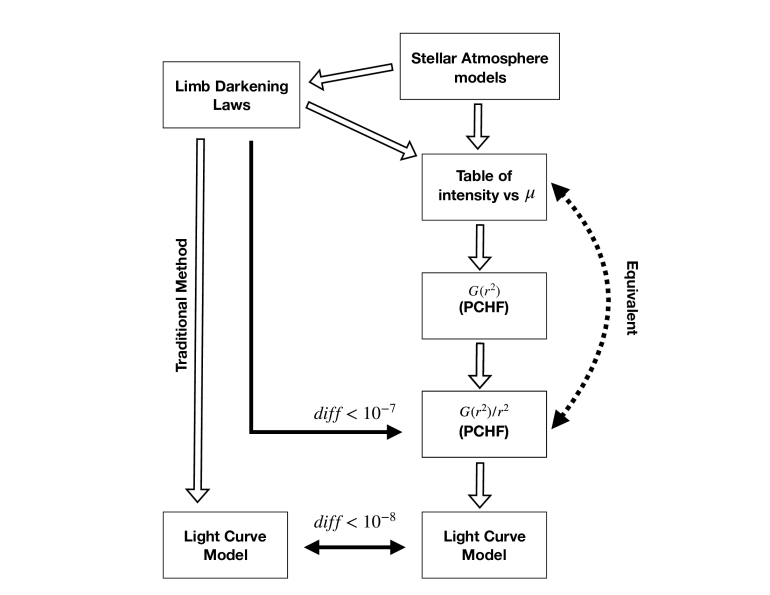
$G$ is an auxiliary function related to the “flux” enclosed within a radius $r^{2}$. In this paper, we will assume that the function $F$ is given by a table of intensity values that define a piecewise linear (PL) function. This table can originate from the values of a parameterized analytic limb darkening law or from a detailed model atmosphere computation. Figure 1 provides a road map for the steps and analysis of this approach. The labeled arrows will be individually discussed.

3 Development of the Method

We begin with a stellar atmosphere model using spherically symmetric geometry that for a given set of stellar parameters (for example effective temperature $T_{\rm eff}$, “surface” gravity $\log g$, mass, and metallicity) produces a table of center-to-limb intensity variations integrated over well defined bandpasses. Such tables were produced by Neilson & Lester (2013) for the standard Johnson-Cousins (BVRIHK) filters and the Kepler and CoRoT bandpasses. These tables sampled 1000 equally spaced points of $\mu$, where $\mu=\cos(\theta)$ and $\theta$ is the angle formed between a line-of-sight point on the stellar disk and the center of the stellar disk. 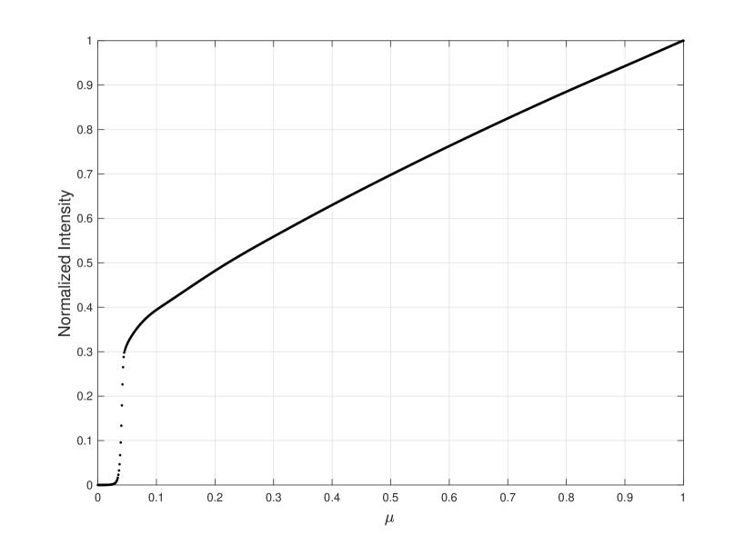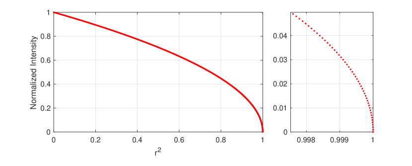If we include the point at the star’s center $(\mu=1)$, which in the normalized case the intensity has a value of 1, we will have a table of size 1001. The graph of such a table for the model stellar atmosphere with parameters of effective temperature $T_{\rm eff}=5700K$, gravity of $\log(g)=4.5$ a mass of $M=1.1\,M_{\odot}$, and solar metallicity is shown in Figure 2. Note the cliff in the intensities near the limb (e.g. $\mu\approx 0$). This feature, which is a consequence of the spherical geometry and thus is not present in the center-to-limb intensity variations computed from model atmospheres that assume plane-parallel geometry, is not reproduced by most simple parameterized limb darkening laws.

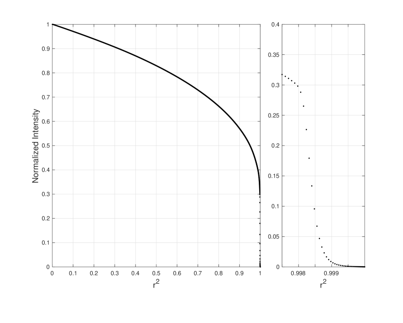
Our goal is to apply the theory of Appendix B in ${\rm Paper~{}I}$ (reproduced here for reader convenience in Appendix A for the flux computation and Appendix B for the R-M effect) to these stellar atmosphere tables, expeditiously producing light curves and models of the R-M effect. The first step is to change the independent variable $\mu$ to $r^{2}$ using the relationship $r^{2}=1-\mu^{2}$. This does not change the intensity values, but rather re-indexes them by $r^{2}$. Since the independent variable in the new table is decreasing, we will now reverse the order so that the new independent variable is increasing. By using linear interpolation between the table values, we can construct a PL function, ${\rm Intensity}=I_{\rm PL}(r^{2})$, which is a continuous function (an example is shown in Figure 3).
To quickly produce interpolated values for a given $r^{2}$, we need to identify the subinterval containing $r^{2}$ where $r_{i}^{2}\leq r^{2}<r_{i+1}^{2}$. This index is given by

$$\begin{aligned} i=N_{\mu}-{\rm ceiling}\big{[}(N_{\mu}-1)\sqrt{1-r^{2}}\big{]}\end{aligned}$$ (8)

where $N_{\mu}$ is the length of the table. The next step in the process of building the required 1-forms, is to evaluate the function $G(r^{2})$ at the table values $r_{i}^{2}$, given by Equation (7). This is done recursively:

$$\begin{aligned} G(r_{i+1}^{2})=G(r_{i}^{2})+\frac{1}{2}\int\displaylimits_{r_{i}^{2}}^{r_{i+1}^{2}}I(r^{2})d(r^{2})\end{aligned}$$ (9)

Since the normalized intensity $I_{\rm PL}(r^{2})$ is a PL function in $r^{2}$, these integrals can be evaluated exactly by using the midpoint rule (Gaussian 1-point). In addition, we can compute the derivative of the integral $G(r^{2})$ with respect to $r^{2}$ analytically:

$$\begin{aligned} \frac{d}{d(r^{2})}G(r^{2})=\frac{1}{2}I(r^{2})\end{aligned}$$ (10)

Thus, we now have a new table with 3 rows. The first row consists of the $r_{i}^{2}$ values, the second row contains the $G(r_{i}^{2})$ values, and the third row contains the derivative of the second row with respect to the first row, or $\frac{1}{2}I(r_{i}^{2})$. Note that the first row together with twice the third row reproduces the original intensity as a function of $r^{2}$. 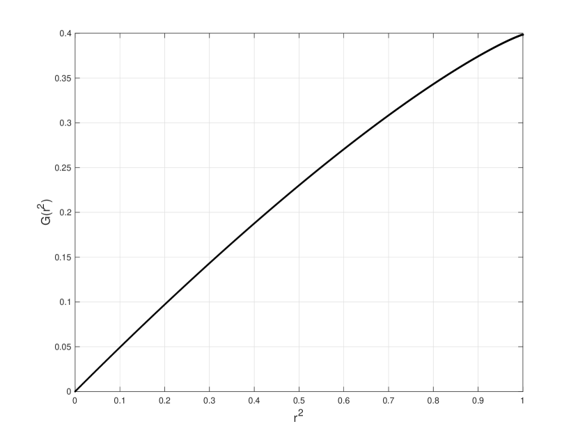This implies that this step resulted in no loss of information. The new table defines a smooth function $G_{\rm PCH}(r^{2})$ using piecewise cubic Hermit (PCH) interpolation for intermediate values (see Appendix C for a thorough discussion). From Equation (6), $G_{\rm PCH}(r^{2})$ now defines the 1-forms required by the R-M effect computation (Figure 4). The final step is to compute $G(r^{2})/r^{2}$, which is needed to compute the 1-form (see the top line in Equation 6) that is required for the light curve computation. For values at each $r_{i}^{2}$, a simple division suffices, except when $r_{i}^{2}=0$. The value at zero is defined by the limit as $r^{2}$ goes to zero, and is computed in Appendix C, giving a value of $\frac{1}{2}I(0)$. The derivatives with respect to $r^{2}$ are computed analytically, except at $r_{i}^{2}=0$:

$$\begin{aligned} \frac{d}{d(r^{2})}\frac{G(r^{2})}{r^{2}}={1\over r^{2}}\bigg{[}\frac{1}{2}I(r^{2})-\frac{G(r^{2})}{r^{2}}\bigg{]}\end{aligned}$$ (11)

Here, the value is, again, defined by the limit as $r^{2}$ approaches zero and is detailed in Appendix C. This limit of the derivative has the value zero.

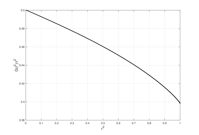
Since we know both the values and the derivatives of $G(r^{2})/r^{2}$, this function may be expressed as a PCH function which we will denote as $G_{\rm PCH}(r^{2})/r^{2}$ (see Figure 5). From Equation (6), $G_{\rm PCH}(r^{2})/r^{2}$ now defines the last 1-forms required by both the light curve and the R-M effect computation. This process converts the given $I_{\rm PL}(r^{2})$ into $G_{\rm PCH}(r^{2})/r^{2}$ which defines the 1-form required for the light curve computation. The top line of Equation (6) is

$$\begin{aligned} d\wedge\bigg{[}-y\frac{G(r^{2})}{r^{2}},x\frac{G(r^{2})}{r^{2}}\bigg{]}=I(r^{2})\end{aligned}$$

In Appendix C we show that the values of the exterior derivative at $r_{i}^{2}$ are equal to the values of the intensity at those same $r_{i}^{2}$ values. Thus, there is no loss of information as the original table can be reconstructed from $G_{\rm PCH}(r^{2})/r^{2}$.
In summary, to efficiently compute light curves from tables of model atmosphere specific intensities, those tables must be in the form of $G_{\rm PCH}(r^{2})/r^{2}$, which can be computed ahead of time. Then, from Equation (4) and Equation (6), the path integrands are now a simple product of a PCH function and sines and cosines. For a given value of $r^{2}$, Equation (8) provides the row index in the table so searching the table is not required.

3.1 Defining the Stellar Radius

The definition of what the “stellar radius” is for a model atmosphere with spherical symmetry merits some discussion. What is often done is to define the radial shell where $r=1.000$ to be where the Rosseland mean optical depth $\tau_{R}$ reaches some critical value. In the SAtlas models, used by Neilson & Lester (2013) to produce the grid of models we are using here, $\tau_{R}=2/3$ is set as the critical value (Lester & Neilson 2008). Alternatively, the PHOENIX models use $\tau_{\rm std}=1$, where $\tau_{\rm std}$ is the optical depth in the continuum at $1.2\mu m$ (Hauschildt et al. 1999). The resulting model atmospheres are insensitive to the precise choice of this critical value (Lester & Neilson 2008). As a practical matter, there is some light coming from beyond the $r=1.000$ shell, so a small number of additional shells are added. For example, in the case of the PHOENIX models as applied to Procyon, the outermost shell extended to $\approx 0.4\%$ beyond the $\tau_{R}=1$ shell (Aufdenberg, Ludwig & Kervella 2005). The “radiation field” $I(\mu,\lambda)$ then refers to the angular distribution of the intensities emerging from the outermost model layer (Aufdenberg, Ludwig & Kervella 2005). As a result of this small extension, the $r=1.000$ radial coordinate defined to be where the optical depth reaches the critical value will not occur at $\mu=0$ in a spherically symmetric model atmosphere, but rather at the $\mu$ value where the slope of the intensity profile is the steepest (see Espinoza & Jordán 2015 and cited references). Indeed, when fitting limb darkening laws to intensity profiles from PHOENIX models, Espinoza & Jordán (2015) put $\mu=0$ at the angle where the intensity profile is the steepest and renormalized the angles. By doing so, the simple limb darkening laws can fit the renormalized profiles much better. On the other hand, the details of what happens near the limb are lost. In our method, such a renormalization is not needed; $\mu=0$ is not reset to the location where the intensity drop off is steepest (nor is it where $\tau=2/3$ or $r=1.000$). It corresponds to a radial coordinate that is very slightly greater than 1.000, in accord with the intensities tabulated by Neilson & Lester (2013) from the SAtlas models. If one chooses $r^{2}$ to be the independent variable, as we do here, then the integration effectively proceeds from the center of the apparent disk (where $r^{2}=0$) outwards in the radial coordinate until the intensity drops to zero, wherever that radial coordinate may be. Thus the use of $r^{2}$ as the radial coordinate effectively decouples the method from the precise definition of the stellar ”radius”.

4 Numerical Properties of the Table

While the Atmosphere Table Method (ATM) follows the theory described in Appendices A and C, the implementation needs to be checked. The first test was accomplished when it was shown that the original stellar atmosphere table could be recovered without loss of information from the table defining $G_{\rm PCH}(r^{2})/r^{2}$ as predicted by the theory. For the next implementation test, we turn to the QL. As we have previously shown, the QL may be written in a dot product form as detailed in ${\rm Paper~{}I}$. That form is given by:

$$\begin{aligned} &I(\mu)/I_{0}=\bm{C}\bm{\cdot}\bm{\Psi}\\ &\text{where }\\ &\bm{C}=\big{[}\big{(}1-(c_{1}+c_{2})\big{)},(c_{1}+2c_{2}),-c_{2}\big{]}\text{~{}~{}and~{}~{}}\bm{\Psi}=\big{[}\bm{1},\mu,\mu^{2}\big{]}\\ \end{aligned}$$ (12)

Here, $\bm{C}$ is a constant vector made from the standard QL coefficients and $\bm{\Psi}$ is a set of basis functions defining the law. The advantage of this form is that the function $G(r^{2})/r^{2}$ has a simple analytic form for each basis function, is independent of the paths to be integrated over (system geometry), and is independent of the law parameters. Equations (4) and (6) give the expression for the path integrands, and these equations show the central role of the function $G(r^{2})/r^{2}$. Once the paths are given, the path integrals can be evaluated, again, independent of the law parameters. This allows for modeling with several different wavelengths without re-computing the paths or the path integrals. For most limb darkening laws we have a listing, in Table 1 of ${\rm Paper~{}I}$, of the analytic form of $G(r^{2})/r^{2}$ for the law’s basis functions. For the QL we have:

$$\begin{aligned} &G(r^{2})/r^{2}{\rm~{}for~{}}\bm{1}\text{~{}is given by~{}}\frac{1}{2}\\ &G(r^{2})/r^{2}{\rm~{}for~{}}\mu\text{ is given by }(1-\mu^{3})/(3r^{2})\\ &G(r^{2})/r^{2}{\rm~{}for~{}}\mu^{2}\text{ is given by }(\frac{1}{2}-\frac{r^{2}}{4})\\ \end{aligned}$$ (13)

The ATM also produces a $G_{\rm PCH}(r^{2})/r^{2}$ for each of the QL basis functions, which can be compared to the QL’s analytic forms. This comparison is independent of the paths (system geometry) and the law parameters. 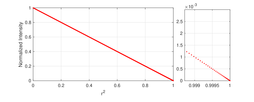The first QL basis function, $\bm{1}$, results in the constant functions of the independent variable $r^{2}$ and thus $G_{\rm PCH}(r^{2})/r^{2}$ is computed exactly to have the value of $\frac{1}{2}$. 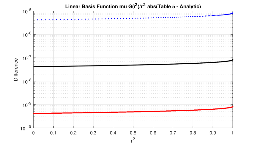The second QL basis function results in the graph, shown in Figure 6, of the normalized intensity with respect to $r^{2}$. Since the PL function, ${\rm Intensity}=I_{\rm PL}(r^{2})$, shows an obvious curvature, the difference between this PL approximation and the analytic form of the QL linear basis function is $O(h^{2})$, where $h$ is the subinterval size that depends on the number of points in the table (see Figure 7). The basis function $\mu^{2}$ results in a linear function of the independent variable $r^{2}$ (Figure 8), and hence $G(r^{2})/r^{2}$ is computed exactly to the precision of the machine. It is only the linear basis function which produces any difference with the analytic form in the development of the basis of 1-forms required for the construction of a light curve using the ATM. If the table size is 1001, then the difference between the model atmosphere’s $G_{\rm PCH}(r^{2})/r^{2}$ and the QL’s analytic form of $G(r^{2})/r^{2}$ for the linear basis function is smaller than $10^{-7}$. This, again, is independent of all system geometries of spherical bodies and of all QL parameters.

5 Computation of the Flux Fraction

The next step in the analysis is to find the flux fraction. This requires the computation of the path integral given in Equation 4, the domain of which is the boundary of the visible portion of the eclipsed body. ${\rm Paper~{}I}$ gives a thorough discussion on how to find the visible boundary, and we summerize here a few key points. This boundary consists of portions of the boundary of the obscuring disks and portions of the boundary of the eclipsed disk. These bounding circular arcs are parametrized by the subtended central angle. For the $i_{th}$ disk centered at $\big{(}X_{{\rm CTR}_{i}},Y_{{\rm CTR}_{i}}\big{)}$ we have:

$$\begin{aligned} &x=R_{i}\cos{\varphi_{i}}+X_{{\rm CTR}_{i}}\\ &y=R_{i}\sin{\varphi_{i}}+Y_{{\rm CTR}_{i}}\end{aligned}$$ (14)

where $R_{i}$ is the radius with center $\big{(}X_{{\rm CTR}_{i}},Y_{{\rm CTR}_{i}}\big{)}$ and the limits on $\varphi$ are $\big{[}\varphi_{0},\varphi_{1}\big{]}$. Switching to the coordinates of the eclipsed body, $M$, in units of the eclipsed body’s radius, we obtain:

$$\begin{aligned} &x=\big{[}R_{i}\cos{\varphi_{i}}+\big{(}X_{{\rm CTR}_{i}}-X_{{\rm CTR}_{M}}\big{)}\big{]}/R_{M}\\ &y=\big{[}R_{i}\sin{\varphi_{i}}+\big{(}Y_{{\rm CTR}_{i}}-Y_{{\rm CTR}_{M}}\big{)}\big{]}/R_{M}\\ \end{aligned}$$ (15)

where we use the same parameter and parameter limits as before. Finally, the orientation of these various parametrized arcs must be consistent with the orientation of the boundary of the eclipsed body. This requires that for those arcs derived from occulting bodies, the limits of integration be switched, or that the path integrals of those arcs be multiplied by $-1$. Thus,

$$\begin{aligned} \oint\displaylimits_{\partial D_{\rm{vis}}}\big{[}P,Q\big{]}\bm{\cdot}\big{[}x^{\prime},y^{\prime}\big{]}d\varphi=\sum_{i=1}^{\rm{\#~{}of~{}Arcs}}(\pm 1)\int\displaylimits_{\varphi_{0}}^{\varphi_{1}}\big{[}P,Q\big{]}\bm{\cdot}\big{[}x^{\prime}_{i},y^{\prime}_{i}\big{]}d\varphi\end{aligned}$$ (16)

where $\pm 1$ is the orientation. If we now focus on one of these integrals using the top line of Equation 6 to define $\big{[}P,Q\big{]}$, we obtain:

$$\begin{aligned} \int\displaylimits_{\varphi_{0}}^{\varphi_{1}}\bigg{[}-y\frac{G(r^{2})}{r^{2}},x\frac{G(r^{2})}{r^{2}}\bigg{]}\bm{\cdot}\big{[}x^{\prime},y^{\prime}\big{]}d\varphi=\int\displaylimits_{\varphi_{0}}^{\varphi_{1}}\frac{G(r^{2})}{r^{2}}\big{(}-yx^{\prime}+xy^{\prime}\big{)}d\varphi\end{aligned}$$ (17)

The first term on the right hand side is simply the PCH function described by the ATM and is easily evaluated using Equation (8) to find the table row to use for computing the PCH interpolant for the given $r^{2}$ (See appendix C). The second term is simply a function of $\sin(\varphi),\cos(\varphi)$ and a constant. Therefore, the system’s geometry will determine the various path integrals to be evaluated.

We evaluate the definite integrals in Equation (17) by Gaussian quadrature. Following the procedures outlined in ${\rm Paper~{}I}$, we divide each integration interval into several “panels”, with the number of panels given by

$$\begin{aligned} N_{\rm opt}={\rm NINT}[(5p\Delta\phi+1)T_{\rm ATM}]\end{aligned}$$ (18)

where $p$ is the ratio of the radii ($R_{\rm front}/R_{\rm back}$), and $T_{\rm ATM}$ is a “tolerance” parameter. Note that this definition of $N_{\rm opt}$ is similar, but not identical to the definition from ${\rm Paper~{}I}$. For clarity, we use the notation $T_{\rm ATM}$ for the tolerance parameter of the new method, and $T$ for the tolerance parameter of the method in ${\rm Paper~{}I}$. After the number of panels is set, $N_{\rm opt}$-point Gaussian quadrature is used up to $N_{\rm opt}=64$. If $N_{\rm opt}>64$, then we use $N_{\rm opt}/m$-point Gaussian quadrature on $m$ equal sub-intervals, where $N_{\rm opt}/m$ is as large as possible without exceeding 64 (if $N_{\rm opt}/m$ is not an integer, $N_{\rm opt}$ is set to the value of the next multiple of $m$ that is larger than $N_{\rm opt}$).

6 Numerical Speed and Accuracy of the new Method

Our ATM has two main sources of numerical uncertainty. In the first case, the definite integrals in Equation (17) are evaluated using Gaussian quadrature, so there is a “quadrature error” associated with that. In ${\rm Paper~{}I}$ we showed, using standard analysis techniques, that the quadrature error gets smaller when the tolerance (e.g. the number of integration panels) is increased, so one can adjust the tolerance $T$ to achieve any target uncertainty on the flux fraction (for example, using $T=128$ results in a (fractional) quadrature error of $\approx 10^{-12}$).

In the second case, there is a “table error” which has two contributions: (i) errors owing to the fact that the center-to-limb intensity values are tabulated at a finite number of points, and (ii) errors in the theoretical model atmosphere intensities owing to inexact treatment of key physical processes and uncertainties in the input atomic data and/or round-off errors in the tabulated values.

There are a few ways to estimate or compute the table error. A relatively trivial way is to compute tables of various lengths using an analytic limb darkening law. Using these mock tables, we can compute a light curve and compare that light curve to a light curve computed using the method of ${\rm Paper~{}I}$ (using $T=128$ so that the quadrature error is minimal). Since the intensity profile is approximated by a PL function $I_{\rm PL}(r^{2})$, the table error should scale $O(h^{2})$ where $h=1/N_{\mu}$ is the subinterval size between tabulated values of the angle $\mu$ (assuming equally spaced values). The scale factor in the error estimate is related to the second derivative of the function, namely $I^{\prime\prime}(\xi)$ for some (unknown) $\xi$ in the interval. Thus, the table error will depend on the curvature of the center-to-limb intensity variations. Since the common analytic limb darkening laws (e.g. quadratic, square root, or logarithmic) have similar curvatures from center-to-limb, the magnitude of the table error should not depend strongly on which analytic limb darkening law is used. Furthermore, since these analytic limb darkening laws produce center-to-limb variations that have less curvature than what is computed from the model atmospheres that use spherical geometry, the measurements of the table error for these analytic laws will yield a “floor” for the table error for a table of length $N_{\mu}$.

When computing the flux fraction for the case of two overlapping bodies, two important quantities are $p$, which is the ratio of the radii and $z$, which is the separation of the centers on the POS, normalized to the radius of the back body. Following ${\rm Paper~{}I}$, we divided the ($p$,$z$) plane into a $2800\times 2800$ grid, where $0<p\leq 3.5$ and $0<z\leq 3.5$. For this exercise, we computed mock tables of various lengths using the QL, the square root law, and the logarithmic law. At each grid point in the ($p$,$z$) plane (excluding the trivial cases of no overlap or total eclipses), we computed the flux fraction using the method of ${\rm Paper~{}I}$ with $T=128$, and the new method outlined here with $T_{\rm ATM}=128$, and found the absolute value of the differences $\Delta$. 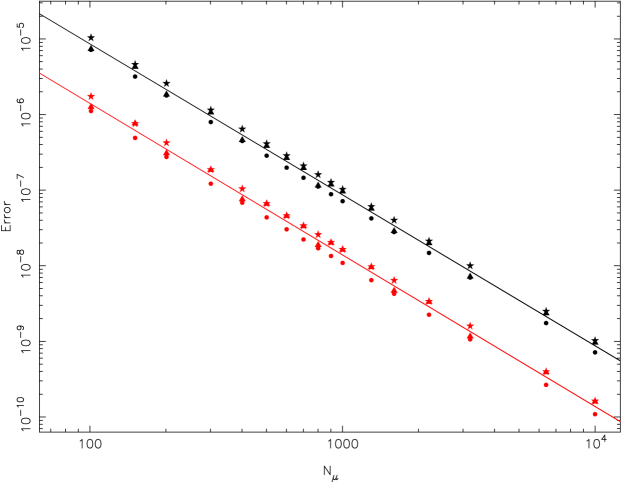For each table, we then recorded the median absolute difference $\Delta_{\rm med}$ and the maximum absolute difference $\Delta_{\rm max}$ in the grid. Figure 9 shows these differences for the various limb darkening laws as a function of the table size $N_{\mu}$. The maximum differences are well described by the power law function $\Delta_{\rm max}=0.08459N_{\mu}^{-1.9964}$ and the median differences are well described by the power law function $\Delta_{\rm med}=0.01437N_{\mu}^{-2.0047}$. Thus, as expected, the errors show the expected behavior where a doubling of the table size reduces the error by a factor of 4. In addition, the magnitude of the table error for a given $N_{\mu}$ does not depend strongly on what analytic limb darkeing law was used. For a table length of $N_{\mu}=1000$ the table errors are $\lesssim 10^{-7}$.

Turning to the tables of model atmosphere intensities computed by Neilson & Lester (2013), we don’t have an easy or practical way to estimate errors in the intensities caused by imperfect atomic data or inexact treatment of the various physical processes. If however, uncertainties in the intensities were available, we can estimate the uncertainties in the flux fractions. The details are somewhat involved, and are given in Appendix D. Neilson & Lester (2013) published 918 tables over a range of temperatures, gravities, and central masses. All of these tables have a length of $N_{\mu}=1001$ when the intensity at the disk center ($\mu=1$) is included. If the uncertainties in the intensities are normally distributed with a mean of zero and a standard deviation of $\sigma$, the maximum error in the flux fraction for the Kepler band is about $0.077\sigma$ for the Neilson & Lester (2013) tables. The intensities are given to 7 digits, and we show in Appendix D that the round-off errors in the tables gives rise to errors on the flux fractions of $\approx 2\times 10^{-9}$. Finally, in Appendix D we estimate the table errors in the flux fractions owing to the finite lengths of the tables. The maximum error estimate for the flux fraction computed from any table in the grid is $2.1\times 10^{-7}$ for the range of $0<p<3$ and $0<z<3$. This is about a factor of 2 larger than what one would get using a mock table of length $N_{\mu}=1000$ computed from an analytic limb darkening law.

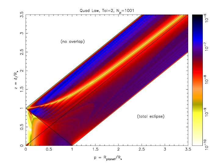
As was the case in ${\rm Paper~{}I}$, there is a tradeoff between the speed of the algorithm and the accuracy of the light curves. Using the QL, we computed grids of flux fraction differences using $T_{\rm ATM}=1$, 2, 4, and 8, and table lengths of $N_{\mu}=1001$, 2001, 4001, and 8001. Figure 10 shows the error map for $T_{\rm ATM}=2$ and $N_{\mu}=1001$. The errors for total transits of small bodies ($p\ll 1$ and $z<1-p$) are generally quite small ($<1\times 10^{-8}$). 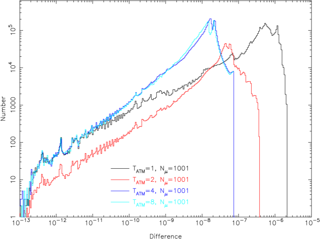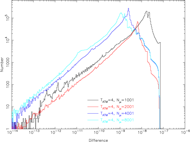For all of the combinations of $T_{\rm ATM}$ and $N_{\mu}$, we recorded the maximum difference and the median difference, excluding the trivial cases of no overlap or a total eclipse. These results are tabulated in Table 1, and Figures 11 and 12 show a few frequency distributions. When $T_{\rm ATM}=1$, the maximum error and the median error hardly change with increasing table length $N_{\mu}$. This suggests that quadrature errors dominate the overall error. When the tolerance is larger (for example $T_{\rm ATM}=4$), increasing the table length results in smaller errors, but only up to a point. When $T_{\rm ATM}\geq 2$ and $N_{\mu}\geq 1001$, the maximum error is $<3.81\times 10^{-7}$ and the median error is $<4.25\times 10^{-8}$.

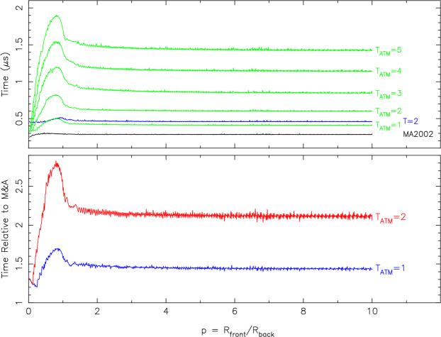
We performed speed tests of the new algorithm using the same procedure as we used  in ${\rm Paper~{}I}$ (for these speed tests, the table was precomputed). The results are shown in Figure 13. The speed of the new algorithm with $T_{\rm ATM}=1$ is similar to the speed of the algorithm of ${\rm Paper~{}I}$ with $T=2$. We used a table length of $N_{\mu}=1001$, but since the algorithm does not require a search of the table, the resulting speed is essentially independent of the length of the table.

7 Light Curve Comparisons

In order to compare transit light curves computed with the ATM outlined above with those computed using analytic limb darkening laws, we chose the table from Neilson & Lester (2013) with the stellar parameters of $T_{\rm eff}=5700$, $\log(g)=4.50$, and mass $M=1.1M_{\odot}$ as the starting point. For this particular combination of mass and gravity the stellar radius is $R=0.97663\,R_{\odot}$. We then placed a planet with a mass of $M_{\rm planet}=0.0011\,M_{\odot}$ and radius of $R_{\rm planet}=0.097633\,R_{\odot}$ in a circular orbit with a period of 10 days. For the light curves, we computed transits in the Kepler, $B$, and $H$ bandpasses. For each filter, a grid of models was computed using impact parameters between 0 and 1 in steps of 0.01. As discussed above, the relative error of these light curves is $\lesssim 2\times 10^{-7}$ in units of the normalized flux.

The grids of light curves from the ATM were fit with models that used the QL with the Kipping (2013) reparameterization of the coefficients, the Power-2 law using the Maxted (2018) reparameterization of the coefficients, and the Claret 4-parameter law, all computed using the methods of ${\rm Paper~{}I}$. We did not add any noise to the grids of light curves. At each impact parameter, the limb darkening coefficients, the planet’s radius, and the the inclination were optimized using a downhill simplex “amoeba” algorithm. 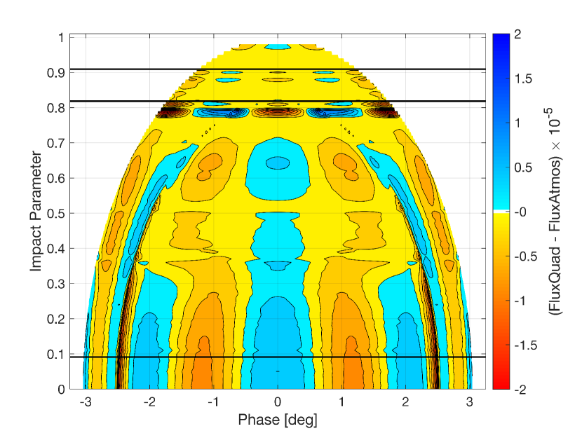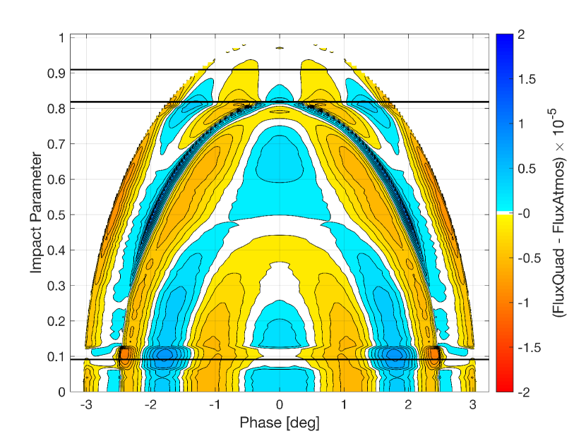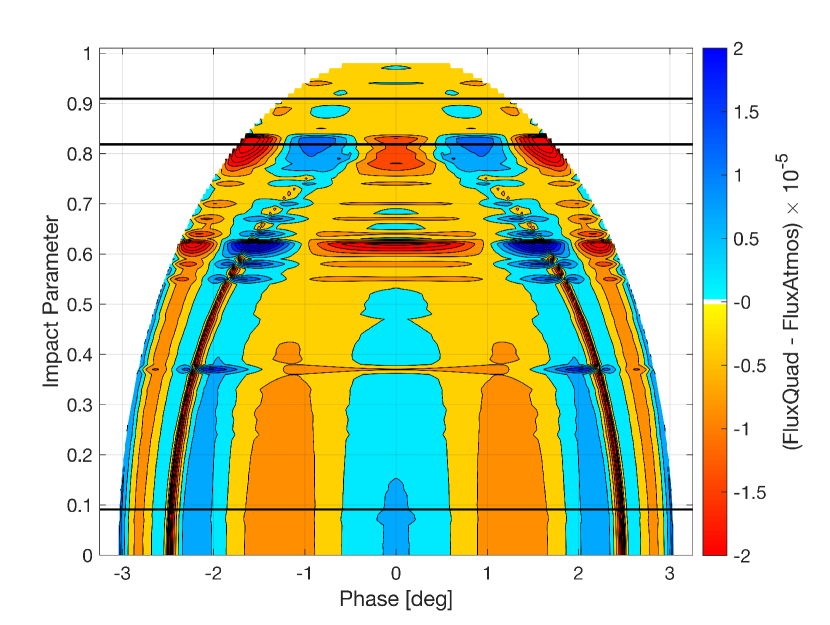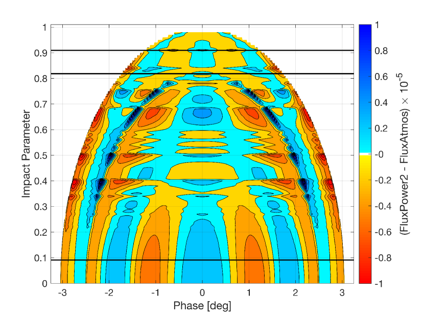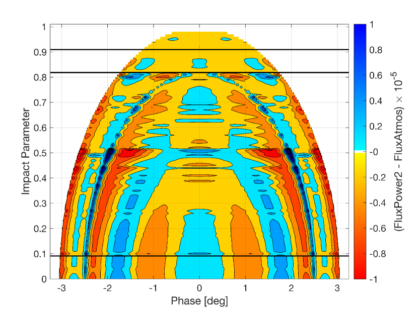Figures 14, 15, and 16 show the light curve residuals for the QL models as a function the impact parameter for the Kepler, $B$, and $H$ bandpasses, respectively. In general, the residuals rise and fall several times across the transit, and depend on the impact parameter of the input model. 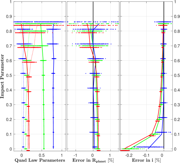Figure 17 shows, for each impact parameter in the grid, the optimal QL coefficients, the relative error in the planet radius, and the relative error in the inclination. The optimal limb darkening coefficients depend on the impact parameter—this has been previously discussed in Neilson et al. (2017), Howarth (2011), Kipping & Bakos (2011a), and Kipping & Bakos (2011b). Likewise, the relative error in the planet’s radius and the relative error in the inclination also depend on the impact parameter. Furthermore, these relative errors also vary with bandpass. In the case of the $H$ bandpass, the maximum flux difference from Figure 16 is about 20 ppm (1 part in 50,000). More importantly, the relative error in the planet’s radius for impact parameters $<0.85$ is about 0.2% for the worst case as shown in Figure 17. To better understand the behavior of this radius bias, we used a nested sampling algorithm (Skilling, 2006) to estimate the uncertainties in the fitted parameters. This was done for the models at impact parameters 0.0 through 0.8 in steps of 0.1, and also for an impact parameter of 0.85. The nested sampling solutions are shown as the horizontal set of points in Figure 17. Notice how the uncertainties in the radius grow larger as the impact parameter increases.

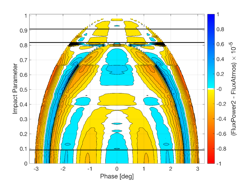
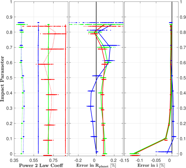
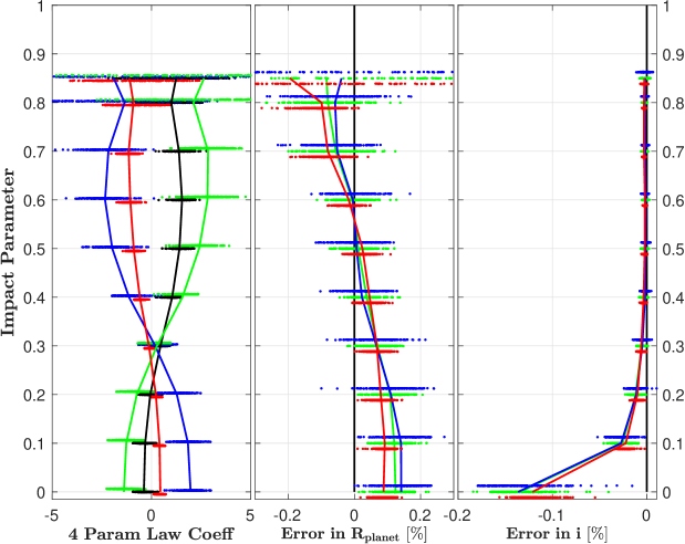
Figures 18, 19, and 20 show the results for the Power-2 law. Note that the range of the color scale has been reduced by a factor of 4 from the QL cases, and that the $B$ and $H$ band graphs exhibit some noise. This noise would imply the Power-2 light curve models are within a digit of the light curve models generated by the ATM. The $B$ and $H$ band model differences with the corresponding ATM models are within ten parts per million. Similar to the case of the QL, Figure 21 shows how the Power-2 law coefficients, relative radius error, and relative inclination error vary with impact parameter. The worst case for the relative planet radius error is $\sim$ 0.1%. The Power-2 law provides an improvement of roughly a factor of two in the radius error over the QL. For brevity, we omit the analogous two-dimensional images showing the transit residuals for the Claret 4-parameter law and just present the fitting results. Figure 22 shows the four limb darkening coefficients for the Kepler band, the error in the planet radius, and the error in the inclination. As seen in the QL and Power-2 law, these are all dependent on the impact parameter. Despite only small deviations in the transit light curve (few ppm), the error in the derived planet radius remains much larger, on the order of $\sim$0.1%, due to various trade-offs among the correlated parameters when optimizing to get the best fit. For the reader’s convenience we provide a Matlab demonstration code that produces a synthetic light curve of a transiting mock planet by using the ATM and the method outlined here and in ${\rm Paper~{}I}$. The code can be downloaded from https://doi.org/10.5281/zenodo.3473851 (Short, 2019).

8 Summary

While limb darkening laws are a convenient parameterization of the limb darkening phenomenon, they can sometimes be inaccurate representations of the stellar intensities. This is particularly true near the limb of the star, where the intensity rapidly drops to zero. In the era of ultra-precise photometry from the Kepler Mission, the use of limb darkening law approximations to match the light curves can lead to systematic biases in the derived model parameters, such as planet radius, inclination (impact parameter), and many other correlated parameters. As shown in previous studies, it would be advantageous to use an actual model stellar atmosphere to give the specific intensities instead of relying on limb darkening law approximations. In general, this has not been done because of the severe computational burden. In this work, we provide a fast method to allow the use of tabulated model stellar atmosphere intensities, thus removing the need for limb darkening laws (and solving for their coefficients).

Our methodology is an extension of the work presented by ${\rm Paper~{}I}$ (Short et al., 2018), where we apply Green’s Theorem to solve the two dimensional integral needed to compute the observed flux during an eclipse or transit. Equations 6 and 7 give the one-forms needed to compute the intensity and R-M effect, and in the present work we show how the function $G(r^{2})$ in these equations can be found numerically given a table of specific intensities from a model atmosphere calculation. More specifically, the input table of radii and intensities is recast as a piecewise linear function, and from that tables of $G(r^{2})$ and $G(r^{2})/r^{2}$ are constructed. These tables uniquely define a piecewise cubic Hermite function which can then be used for interpolation for any intermediate values of $r$. The conversion from the model atmosphere table (C1) to the form of the tables used in computing the values of the integrand (C16) is done once. It is reversible, implying no loss of information. Any error in the computed light curve stems mainly from the sizes of the steps (gaps or intervals) in the tabulated intensities (and of course from the limitations inherent in the stellar atmosphere models themselves). For a two-body eclipse, the method is only a factor of $\sim$ 2 slower than the Mandel & Agol (2002) code, but the inclusion of actual stellar physics and the a priori known level of precision more than compensate for the additional compute time. The light curve or R-M radial velocity curve for any number of overlapping spherical bodies can be computed.

Using the tabulated specific intensities computed with the ATLAS stellar atmosphere models from Neilson & Lester (2013), we make a direct comparison of our atmosphere table method with the traditional quad law and Power-2 limb darkening laws for a hot Jupiter transit. Noting that the best-match quad law coefficients depend on the impact parameter, differences of several tens of ppm are present in the transit. The derived planet radius can be systematically biased by as much as $\sim$ 500 ppm in the H-band, depending on the impact parameter. While this is a small bias, such errors can be problematic as photometric precision continues to improve and as demands on the data increase, e.g., when considering higher-order effects such as planet oblateness, rings, satellite transits, etc. An area where our method may be particularly valuable is transit spectroscopy. A transit depth is wavelength-dependent due to both the planet’s atmosphere and the stellar limb darkening. By eliminating the use of parameterized limb darkening law approximations, we (i) take advantage of the full knowledge of the star’s intensity distribution (which can strongly vary with wavelength) from the stellar atmosphere models, and (ii) remove the degeneracy between planet radius and the empirically-constrained limb darkening coefficients because there are no coefficients in the model - the limb darkening is entirely set by the stellar mass, radius, temperature, and metallicity. Because the limb darkening has no free parameters, the accuracy of the treatment of the limb darkening now depends entirely on the accuracy of the stellar models used.

This current paper describes how to use tabulated stellar atmosphere model intensities instead of limb darkening laws, under the assumption that such a table exists for the desired stellar parameters. Future work involves being able to precisely and efficiently interpolate the input stellar atmosphere tables across values of $T_{\rm eff}$, $\log(g)$ and metallicity.

Appendix A Anti-Exterior Derivatives For Radially Defined Function

Assume $f=f(r^{2})$ is a continuous function on the unit disk (every limb darkening is of that form). Since the 2-form $f(x,y)dxdy$ is a closed form on the unit disk, Poincaré’s Lemma asserts that there exists a 1-form $P(x,y)dx+Q(x,y)dy$ such that

$$d\wedge\big{[}P,Q\big{]}=\frac{\partial Q}{\partial x}-\frac{\partial P}{\partial y}=f(x,y)$$ (A1)

Try $P(x,y)=-yF(r^{2}),~{}~{}Q(x,y)=xF(r^{2})$ for some smooth function $F$ on the unit disk. Then

$$\begin{aligned} &\frac{\partial Q}{\partial x}-\frac{\partial P}{\partial y}=F(r^{2})+2x^{2}\frac{dF(r^{2})}{dr^{2}}+F(r^{2})+2y^{2}\frac{dF(r^{2})}{dr^{2}}\\ &\rm{or}\\ &2F(r^{2})+2r^{2}\frac{dF(r^{2})}{dr^{2}}=f(r^{2})\\ &{\rm or}\\ &\frac{2d\big{(}r^{2}F(r^{2})\big{)}}{dr^{2}}=f(r^{2})\end{aligned}$$ (A2)

integrating $f=f(z)$ with respect to $z$ where $z=r^{2}$, from $0$ to $r^{2}$, gives

$$\begin{aligned} 2r^{2}F(r^{2})=\int\displaylimits_{0}^{r^{2}}f(z)dz\end{aligned}$$

or

$$\begin{aligned} F(r^{2})=\frac{{\int}\displaylimits_{0}^{r^{2}}f(z)dz}{2r^{2}}\end{aligned}$$ (A3)

Thus the 1-forms are $P=-yF(r^{2}),~{}~{}Q=xF(r^{2})$, the exterior derivative of which is $f(r^{2})$.

In the case of the R-M effect, all of the terms in the numerator of Equation (B5), using any of the limb darkening laws, have the 2-form $g=xf(r^{2})$ or $h=yf(r^{2})$ on the unit disk. Try

$$\begin{aligned} &P_{1}(x,y)=0&Q_{1}(x,y)&=G(r^{2})\\ &P_{2}(x,y)=G(r^{2})&Q_{2}(x,y)&=0\\ \end{aligned}$$ (A4)

Therefore,

$$\begin{aligned} &\frac{\partial P_{1}}{\partial y}=0\\ &\frac{\partial Q_{1}}{\partial x}=\frac{dG(r^{2})}{dr^{2}}(2x)=2x\frac{dG(r^{2})}{dr^{2}}=g(x,y)=xf(r^{2})\\ &{\rm or}~{}\frac{dG(r^{2})}{dr^{2}}=\frac{1}{2}f(r^{2})\\ \end{aligned}$$

which we then integrate:

$$\begin{aligned} &G(r^{2})=\frac{1}{2}\int\displaylimits_{0}^{r^{2}}f(z)dz\\ \end{aligned}$$

Hence

$$\begin{aligned} &d\wedge\big{[}0,G(r^{2})\big{]}=xf(r^{2})~{}\rm{and}\\ &d\wedge\big{[}-G(r^{2}),0\big{]}=yf(r^{2})\\ \end{aligned}$$

In summary,

$$\begin{aligned} G(r^{2})=\frac{1}{2}\int\displaylimits_{0}^{r^{2}}f(z)dz\\ \end{aligned}$$ (A5)

where $f=f(r^{2})$ is a continuous function on the unit disk. Then,

$$\begin{aligned} &d\wedge\bigg{[}-y\frac{G(r^{2})}{r^{2}},x\frac{G(r^{2})}{r^{2}}\bigg{]}=f(r^{2})\\ &d\wedge\bigg{[}0,G(r^{2})\bigg{]}=xf(r^{2})\\ &d\wedge\bigg{[}-G(r^{2}),0\bigg{]}=yf(r^{2})\\ \end{aligned}$$ (A6)

We note, again, that Equations (A6) explicitly give the 1-forms $[P,Q]$ for the flux calculation for any limb darkening given by

$$\begin{aligned} I(\mu)/I_{0}=f(r^{2})=f(1-\mu^{2})\end{aligned}$$

(where $f$ is a continuous function on the disk $D$), and for the 1-forms $[P,Q]$ for the R-M effect based on that limb darkening. The specific form of the integral $G$ (Equation A5) will determine if $[P,Q]$ can be expressed in closed form, by a special function, or will require numerical evaluation using Gaussian quadrature.

Appendix B Anti-exterior Derivatives for the Rossiter-McLaughlin Effect

Following the development of the R-M effect from Section 4.2 of ${\rm Paper~{}I}$, define the rotation axis of the star in the dynamic coordinate system $(x,y,z)$, with the observer on the positive $z$-axis, as defined by Equation 1. Note that this differs from the system first defined Hosokawa (1953) and then used again by Giménez (2006a). Since their emphasis was on simple binary systems and planetary transits, their $y$-axis was simply the projection of the orbital pole on the POS. In this work we do not assume a simple two-body system but rather a multi-body system in which

$$\begin{aligned} &\Theta_{\rm rot}\equiv\text{~{}~{}angle in the $(x,y)$ plane from the $y$-axis}\\ &\Phi_{\rm rot}\equiv\text{~{}~{} angle from the $z$-axis colatitude}\end{aligned}$$ (B1)

If the axis of rotation of the star is the $z$-axis, then the right-hand surface velocity field on the unit sphere is given by

$$\begin{aligned} v(x,y,z)=\omega(-y,x,0)\end{aligned}$$ (B2)

where $\omega$ is the angular velocity in radians per day. Note that $\lVert(-y,x,0)\rVert$ is the distance to the axis of rotation (the $z$-axis). Using rotation transformations (orthonormal matrices with determinants equal to 1), move the $z$-axis to the rotation axis described by $(\Theta_{\rm rot},\Phi_{\rm rot})$. Since the transformations are length and orientation-preserving, the transformation of the velocity field is also preserved as the velocity field generated by the right-hand rotation about the axis $(\Theta_{\rm rot},\Phi_{\rm rot})$. The radial velocity function is simply the $z$-component of this velocity field in the dynamic coordinate system. Namely,

$$\begin{aligned} v(x,y)=\omega\bigg{[}\bigg{(}\sin(\Phi_{\rm rot})\cos(\Theta_{\rm rot})\bigg{)}x+\bigg{(}\sin(\Phi_{\rm rot})\sin(\Theta_{\rm rot})\bigg{)}y\bigg{]}\end{aligned}$$ (B3)

for $(x,y)$ being any point on the POS disk normalized to the unit disk. Define:

$$\begin{aligned} &A\equiv\sin(\Phi_{\rm rot})\cos(\Theta_{\rm rot})\\ &B\equiv\sin(\Phi_{\rm rot})\sin(\Theta_{\rm rot})\end{aligned}$$ (B4)

Equation 27 in ${\rm Paper~{}I}$ models the radial velocity perturbation (R-M effect) during an eclipse of the star as follows:

$$\delta RV=\frac{{\iint}\displaylimits_{D_{\rm vis}}(Ax+By)\cdot IdA}{{\iint}\displaylimits_{D_{\rm{vis}}}IdA}=\frac{{\oint}\displaylimits_{\partial D_{\rm vis}}\big{[}P_{\rm RM},Q_{\rm RM}\big{]}\bm{\cdot}\big{[}x^{\prime},y^{\prime}\big{]}d\varphi}{{\oint}\displaylimits_{\partial D_{\rm{vis}}}\big{[}P_{\rm FF},Q_{\rm FF}\big{]}\bm{\cdot}\big{[}x^{\prime},y^{\prime}\big{]}d\varphi}$$ (B5)

The numerator is the rotational velocity field, moderated by the intensity of the star, $I$. The denominator is the normalized intensity. From Equation (A6) we have

$$\begin{aligned} &d\wedge\bigg{[}0,G(r^{2})\bigg{]}=xI(r^{2})\\ &\text{and}\\ &d\wedge\bigg{[}-G(r^{2}),0\bigg{]}=yI(r^{2})\end{aligned}$$ (B6)

Thus,

$$\begin{aligned} &d\wedge\bigg{[}-BG(r^{2}),AG(r^{2})\bigg{]}=\big{(}Ax+By)I(r^{2})\\ \end{aligned}$$ (B7)

Hence

$$\delta RV=\frac{{\oint}\displaylimits_{D_{\rm vis}}G(r^{2})\big{(}-Bx^{\prime}+Ay^{\prime}\big{)}d\varphi}{{\oint}\displaylimits_{D_{\rm vis}}\frac{G(r^{2})}{r^{2}}\big{(}-yx^{\prime}+xy^{\prime}\big{)}d\varphi}$$ (B8)

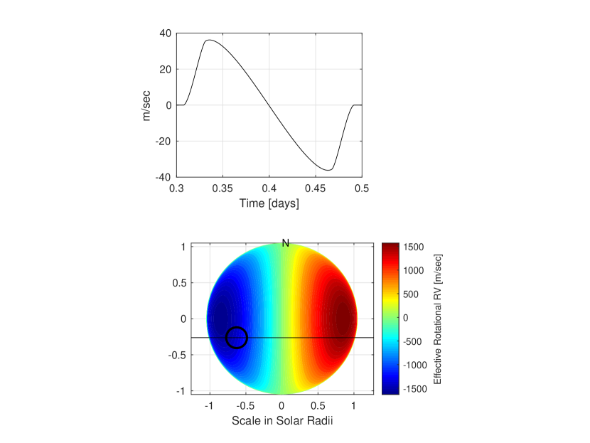
Applying this method to the Hot Jupiter example with the additional parameters: $i=89^{\circ}$, rotation period $=20{\rm~{}days}$, $\Phi_{\rm rot}=90^{\circ}$ (colatitude), and $\Theta_{\rm rot}=0$ (angle from the POS $y$ axis), we obtain the result shown in Figure 23. Note that “$N$” is the north pole of the right handed stellar rotation axis. The black circle is the outline of the planet, and the black line is its orbital track. 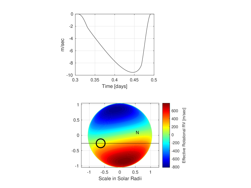If we now change the axis of the stellar rotation to $\Phi_{\rm rot}=30^{\circ}$ (colatitude), and $\Theta_{\rm rot}=-80$ (angle from the POS $y$ axis), we obtain what is shown in Figure 24.

Appendix C Table Defined Functions

Given a table of values (e.g ȧn Atmosphere Intensity table)

$$\begin{aligned} \begin{bmatrix}r_{1}^{2}&r_{2}^{2}&\bm{\ldots}&r_{n}^{2}\\ I_{1}&I_{2}&\bm{\ldots}&I_{n}\\ \end{bmatrix}\end{aligned}$$ (C1)

a piecewise linear function $f_{\rm PL}$ is defined by

$$\begin{aligned} I_{i}=f_{\rm PL}(r_{i}^{2})\end{aligned}$$ (C2)

For intermediate values the intensities are found by linear interpolation. For $r_{i}^{2}<r^{2}<r_{i+1}^{2}$ linear interpolation gives

$$\begin{aligned} &f_{\rm PL}(r^{2})=I_{i}+a(r^{2}-r_{i}^{2})\\ &{\rm where~{}~{}}a=\frac{I_{i+1}-I_{i}}{r_{i+1}^{2}-r_{i}^{2}}\end{aligned}$$ (C3)

Equation (A5) defines an important integration operation on $f_{\rm PL}$, namely

$$\begin{aligned} G(r^{2})=\frac{1}{2}\int\displaylimits_{0}^{r^{2}}I(z)dz\\ \end{aligned}$$ (C4)

To build the table of values we assume $r_{1}^{2}=0$, and for subsequent table values we obtain a recursion formula starting with $G(r_{1}^{2})=0$ and continuing with

$$\begin{aligned} G(r_{j}^{2})=\frac{1}{2}\int\displaylimits_{0}^{r_{j}^{2}}f_{\rm PL}(z)dz=\frac{1}{2}\int\displaylimits_{0}^{r_{j-1}^{2}}f_{\rm PL}(z)dz+\frac{1}{2}\int\displaylimits_{r_{j-1}^{2}}^{r_{j}^{2}}f_{\rm PL}(z)dz\end{aligned}$$ (C5)

or

$$\begin{aligned} G(r_{j}^{2})=G(r_{j-1}^{2})+\frac{1}{2}\int\displaylimits_{r_{j-1}^{2}}^{r_{j}^{2}}f_{\rm PL}(z)dz\end{aligned}$$ (C6)

where $f_{\rm PL}(z)$ is the line segment from $(r_{j-1}^{2},I_{j-1})$ to $(r_{j}^{2},I_{j})$. The value of this integral is given exactly by the mid-point rule (Gaussian 1-point) as

$$\begin{aligned} \frac{1}{2}\int\displaylimits_{r_{j-1}^{2}}^{r_{j}^{2}}f_{\rm PL}(z)dz=\frac{1}{2}\frac{f_{\rm PL}(r_{j-1}^{2})+f_{\rm PL}(r_{j}^{2})}{2}(r_{j}^{2}-r_{j-1}^{2})=\frac{1}{4}(I_{j-1}+I_{j})(r_{j}^{2}-r_{j-1}^{2})\end{aligned}$$ (C7)

In addition, we can compute the derivative of $G$ with respect to $r^{2}$:

$$\begin{aligned} &&\frac{d}{dr^{2}}G(r^{2})=\frac{1}{2}f(r^{2})\\ \end{aligned}$$ (C8)

or for the table values,

$$\begin{aligned} &&\frac{d}{dr^{2}}G(r^{2})\bigg{|}_{r_{i}^{2}}=\frac{1}{2}f(r_{i}^{2})\end{aligned}$$

Thus we obtain a new table based on the function $G(r^{2})$:

$$\begin{aligned} \begin{bmatrix}r_{1}^{2}&r_{2}^{2}&\bm{\ldots}&r_{n}^{2}\\ G(r_{1}^{2})&G(r_{2}^{2})&\bm{\ldots}&G(r_{n}^{2})\\ \frac{1}{2}I_{1}&\frac{1}{2}I_{2}&\bm{\ldots}&\frac{1}{2}I_{n}\end{bmatrix}\end{aligned}$$ (C9)

where the third row is the derivative of the second row with respect to the first row. This table uniquely defines a piecewise cubic Hermit (PCH) function using cubic Hermite interpolation for intermediate values. That is, $G_{\rm PCH}(r_{i}^{2})=G(r_{i}^{2})$, and for $r_{i}^{2}<r^{2}<r_{i+1}^{2}~{}~{}~{}G_{\rm PCH}(r^{2})=\text{cubic Hermite Interpolant}$.

$$\begin{aligned} \begin{tabular}[]{c|lccc}\@add@centering\centering$r_{i}^{2}$&$G(r_{i}^{2})$&&&\\ &&$G^{\prime}(r_{i}^{2})$&&\\ $r_{i}^{2}$&$G(r_{i}^{2})$&&$~{}~{}b$&\\ &&$a$&&$~{}~{}~{}~{}~{}~{}d$\\ $r_{i+1}^{2}$&$G(r_{i+1}^{2})$&&$~{}~{}c$&\\ \\ &&$G^{\prime}(r_{i+1}^{2})$&&\\ $r_{i+1}^{2}$&$G(r_{i+1}^{2})$&&&\\ \end{tabular}\\ \\ \\ \end{aligned}$$ (C10)

where

$$\begin{aligned} a=\frac{G(r_{i+1}^{2})-G(r_{i}^{2})}{r_{i+1}^{2}-r_{i}^{2}}~{},~{}b=\frac{a-G^{\prime}(r_{i}^{2})}{r_{i+1}^{2}-r_{i}^{2}}~{},~{}c=\frac{G^{\prime}(r_{i+1}^{2})-a}{r_{i+1}^{2}-r_{i}^{2}}~{},~{}d=\frac{c-b}{r_{i+1}^{2}-r_{i}^{2}}\end{aligned}$$

From this divided difference table, the cubic interpolating polynomial is given by:

$$\begin{aligned} G_{\rm PCH}(r^{2})=G(r_{i}^{2})+(r^{2}-r_{i}^{2})\bigg{\{}G^{\prime}(r_{i}^{2})+(r^{2}-r_{i}^{2})\bigg{[}b+d(r^{2}-r_{i+1}^{2})\bigg{]}\bigg{\}}\end{aligned}$$ (C11)

From Equation (A6) we also need to construct the PCH function $G_{\rm PCH}(r^{2})/r^{2}$. To do this, we must compute its derivative

$$\begin{aligned} &\frac{d}{dr^{2}}\bigg{(}G(r^{2})/r^{2}\bigg{)}=\frac{G^{\prime}(r^{2})}{r^{2}}-\frac{G(r^{2})}{r^{4}}\\ &\text{and}\\ &\lim_{r^{2}\to 0}\frac{G(r^{2})}{r^{2}},~{}~{}\lim_{r^{2}\to 0}\frac{d}{dr^{2}}\bigg{(}G(r^{2})/r^{2}\bigg{)}\\ \end{aligned}$$ (C12)

The first limit is evaluated by L’Hospital’s Rule:

$$\begin{aligned} &\lim_{r^{2}\to 0}\frac{G(r^{2})}{r^{2}}=&\lim_{r^{2}\to 0}\frac{G^{\prime}(r^{2})}{1}=\frac{1}{2}I(0)\\ \end{aligned}$$ (C13)

to compute the second limit, assume that the intensity is a maximum at $r^{2}=0,$ and that the intensity is smooth at $r^{2}=0$. Expand the intensity about $r^{2}=0$ in a Taylor series:

$$\begin{aligned} I(r^{2})&=I(0)+I^{\prime}(0)r^{2}+O(r^{4})\\ \\ \text{and}\\ G(r^{2})&=\frac{1}{2}\int\displaylimits_{0}^{r^{2}}I(0)+I^{\prime}(0)z+O(z^{2})dz\\ &=\frac{1}{2}\bigg{(}I(0)r^{2}+I^{\prime}(0)\frac{r^{4}}{2}+O(r^{6})\bigg{)}\end{aligned}$$ (C14)

$$\begin{aligned} \lim_{r^{2}\to 0}\frac{G^{\prime}(r^{2})}{r^{2}}-\frac{G(r^{2})}{r^{4}}=\lim_{r^{2}\to 0}\frac{1}{2}\frac{I(r^{2})}{r^{2}}-\frac{1}{2}\bigg{(}\frac{I(0)}{r^{2}}+\frac{I^{\prime}(0)}{2}+O(r^{2})\bigg{)}=\frac{-I^{\prime}(0)}{4}\end{aligned}$$ (C15)

however, $I$ assumes a maximum at $r^{2}=0$, implying that $I^{\prime}(0)=0$. Thus the table representation of $G(r^{2})/r^{2}$ is given by:

$$\begin{aligned} \begin{bmatrix}r_{1}^{2}&r_{2}^{2}&\bm{\ldots}&r_{n}^{2}\\ \frac{1}{2}I(0)&\frac{G(r_{2}^{2})}{r_{2}^{2}}&\bm{\ldots}&\frac{G(r_{n}^{2})}{r_{n}^{2}}\\ 0&\frac{\frac{1}{2}I_{2}}{r_{2}^{2}}-\frac{G(r_{2}^{2})}{r_{2}^{4}}&\bm{\ldots}&\frac{\frac{1}{2}I_{n}}{r_{n}^{2}}-\frac{G(r_{n}^{2})}{r_{n}^{4}}\end{bmatrix}\end{aligned}$$ (C16)

for efficiency, we include two additional table-rows in the code, the interpolation factors $b$ and $d$. This will allow direct use of the cubic interpolating polynomial without computing the difference table.

As a check, we will now evaluate the exterior derivative in Equation 87 of ${\rm Paper~{}I}$:

$$\begin{aligned} &d\wedge\bigg{[}-y\frac{G(r^{2})}{r^{2}},x\frac{G(r^{2})}{r^{2}}\bigg{]}=I(r^{2})\\ \text{the left hand side:}\\ &=\frac{\partial}{\partial x}x\frac{G(r^{2})}{r^{2}}-\frac{\partial}{\partial y}y\frac{G(r^{2})}{r^{2}}\\ &=\frac{G(r^{2})}{r^{2}}+2x^{2}\frac{d}{dr^{2}}\frac{G(r^{2})}{r^{2}}+\frac{G(r^{2})}{r^{2}}+2y^{2}\frac{d}{dr^{2}}\frac{G(r^{2})}{r^{2}}\\ &=2\frac{G(r^{2})}{r^{2}}+2r^{2}\frac{d}{dr^{2}}\frac{G(r^{2})}{r^{2}}=I(r^{2})\end{aligned}$$ (C17)

or in terms of the table representation of $G(r^{2})/r^{2}$ we have

$$\begin{aligned} 2\cdot{\rm row2}+2\cdot{\rm row1}\ast{\rm row3}={\rm Intensity}\end{aligned}$$

where $\ast$ is element by element multiplication. The result is that the manulipation of the table rows in the above manner gives the original intensity to the machine precision.

Finally, we comment on a lesser known issue of modeling eclipses with limb darkening laws where the boundary of the front body crosses the back body’s center. The limb-darkening laws are not models of stellar intensity, but rather are models of time and azimuthal averaged stellar intensities. This averaging eliminates the time varying processes such as spots, granulation, etc. The averaging produces a smooth POS stellar intensity model with no angular dependence. Thus, the derivative of this two dimensional function exists at the star’s center and is angular-independent there. It then follows that the partial derivatives with respect to x and y exist at the center and must be zero, implying that the center is a critical point. Because the stellar intensity increases as one moves towards the center, the center must be a maximum for the two dimensional stellar intensity function. Thus for its one dimensional cross-section the derivative at $\mu=1$ (the center) is zero. In contrast, for the standard limb darkening laws the one-sided derivative at the center is not zero. This implies that the limb darkening model applied to the POS is not differentiable at the center. If we are using the Mandel-Agol algorithm to model an eclipse where the center of the back body is covered, at least two different special function approximations are required (this is the case of crossing from “region 2” to “region 8” or crossing from “region 3” to “region 9”, see Figure 6 in ${\rm Paper~{}I}$). This may result in an error in the computation of the transit profile (see Figure 17 in ${\rm Paper~{}I}$). Note that if a numerical integration scheme is used instead of a set of special functions, the discontinuity at the center does not lead to errors in the flux. That numerical scheme may use tabulated stellar intensities (this paper) or the limb darkening laws themselves (e.g. ${\rm Paper~{}I}$). It is the use of the special functions and the matching of boundary conditions that leads to the error in the transit profile.

Appendix D Error Analysis for the Atmosphere Table Method

Suppose we have an error estimate for the entries of a stellar atmosphere table. We can ask two questions about the error associated with that table. The first question is, what is the resulting maximum error for the light curve of an eclipse computed from such a table? The second question is, given an atmosphere table of size $N_{\mu}$, what is the maximum absolute error generated by using the table PL function in the computation of a light curve?

To address the first question, assume that the table center-to-limb intensities are given by

$$\begin{aligned} I(\mu_{i})=I_{\rm AT}(\mu_{i})+E(\mu_{i})\end{aligned}$$ (D1)

where $E$ is an error distribution of intensities, having a mean 0 and a variance $\sigma_{E}^{2}$. Further assume that the Central Limit Theorem applies for $N\ll N_{\mu}$ and that the mean of the sum of $N_{\mu}$ error distributions closely approximates a normal distribution with a mean 0 and variance $\sigma_{E}^{2}/N_{\mu}$. For any selection of errors using the prescribed distribution, $I$ is just a new stellar atmosphere table, and as such we may apply the methodology of Appendix C. First, the independent variable $\mu$ is changed to $r^{2}$. Equation C4 shows that the function $G(r^{2})$ is linear in $I$, which implies

$$\begin{aligned} &G_{I}(r^{2})=G_{\rm AT}(r^{2})+G_{E}(r^{2})\\ &\frac{G_{I}(r^{2})}{r^{2}}=\frac{G_{\rm AT}(r^{2})}{r^{2}}+\frac{G_{E}(r^{2})}{r^{2}}\end{aligned}$$ (D2)

Finally, computing the flux (Equations 4, 16, and 17) we note that flux is linear with respect to the function $G/r^{2}$, thus we obtain for the Flux $\cal{F}$:

where $(p,z)$ describes the geometry of the eclipsing system as in Section 5 and ${\rm Paper~{}I}$. The flux is then normalized by the flux of the unobstructed body, which is given by:

Our immediate goal is to reduce $G_{E}(1)$ to a small fraction of $G_{\rm AT}(1)$, so that ${\cal{F}}_{0}$ is simply $2\pi G_{\rm AT}(1)$. Applying the trapezoid rule to $G_{E}(1)$ (which is exact since E(z) is a PL function), we obtain

$$\begin{aligned} G_{E}(1)=\frac{1}{2}\int\displaylimits_{0}^{1}E(z)dz=\frac{\frac{1}{2}\bigg{\{}\bigg{[}\sum\displaylimits_{i=2}^{N_{\mu}-1}E(\mu_{i})\bigg{]}+\frac{1}{2}\bigg{[}E(0)+E(1)\bigg{]}\bigg{\}}}{N_{\mu}-1}\end{aligned}$$ (D3)

Since $I(1)=1$ then for all atmosphere tables $E(1)=0$:

$$\begin{aligned} &G_{E}(1)=\frac{\frac{1}{2}\bigg{\{}\bigg{[}\sum\displaylimits_{i=2}^{N_{\mu}-1}E(\mu_{i})\bigg{]}+\frac{1}{2}\bigg{[}E(0)\bigg{]}\bigg{\}}}{N_{\mu}-1}\end{aligned}$$ (D4)

or

Case 1: $E$ is the normal distribution with mean 0 and standard deviation $\sigma$. $E$ can be written as $E=\sigma U$, where $U$ is the unit normal distribution having mean 0 and standard deviation 1.

$$\begin{aligned} &\text{MaxLightCurveError}={\rm max_{(p~{}and~{}z)}}\bigg{\lvert}\frac{\sigma{\cal{F}}_{\rm U}(p,z)}{{\cal{F}}_{0}}\bigg{\rvert}=&\frac{\sigma}{2\pi G_{\rm AT}(1)}{\rm max_{(p~{}and~{}z)}}\bigg{\lvert}{\cal{F}}_{\rm U}(p,z)\bigg{\rvert}\end{aligned}$$ (D7)

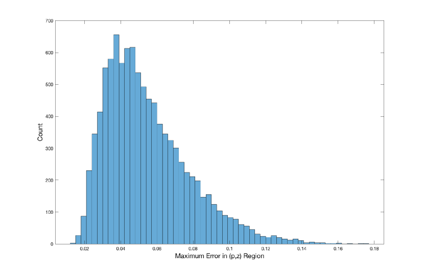
Only the first term, ${\sigma}/[2\pi G_{\rm AT}(1)]$, depends on the particular atmosphere table and its size. For the second term, 10,000 tables were constructed for the table size $N_{\mu}=1001$. For each of these, the ${\rm max_{(p~{}and~{}z)}}\lvert{\cal{F}}_{\rm U}(p,z)\rvert$ was computed. Figure 25 shows a histogram of the resulting light curve maxima. For these 10,000 sample tables of the unit normal distribution, the maximum absolute value error was 0.1748. Since the error modeled by the unit normal distribution can have arbitrary large values - even if very rare - the actual maximum does not exist. Truncating the normal distribution at a few $\sigma$ would solve this problem. We then have

$$\begin{aligned} \text{MaxLightCurveError}=\frac{\sigma}{2\pi G_{\rm AT}(1)}{\rm max_{(p~{}and~{}z)}}\bigg{\lvert}{\cal{F}}_{\rm U}(p,z)\bigg{\rvert}=\frac{\sigma}{2\pi G_{\rm AT}(1)}0.18=\frac{0.18}{{\cal{F}}_{0}}\sigma\end{aligned}$$ (D8)

For the set of 918 atmosphere tables by Neilson & Lester (2013) in the $Kepler$ band, the bounds on ${\cal{F}}_{0}$ are $2.330<{\cal{F}}_{0}<2.652$, giving the result: $\text{\it Kepler~{}}\text{MaxLightCurveError}=0.077\sigma$ where $\sigma$ is the standard deviation of the original table error.

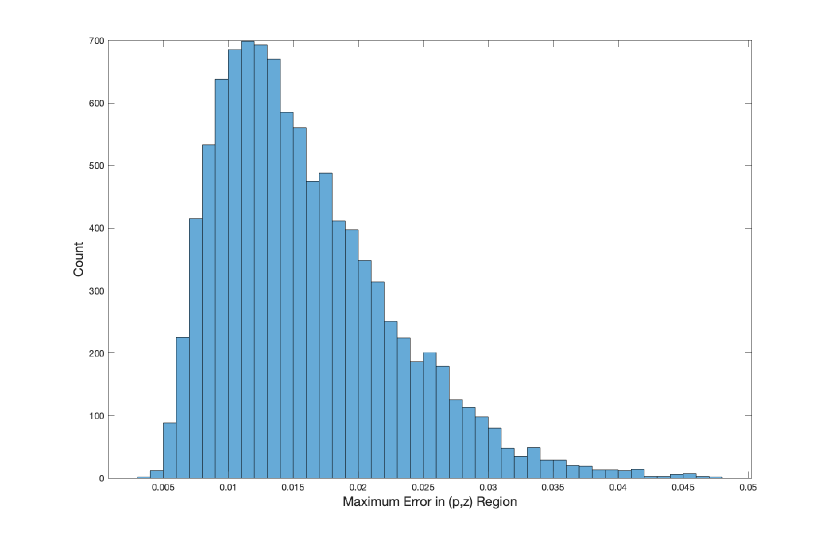
Case 2: $E$ is the uniform distribution on $[-0.5,0.5]\epsilon$ with mean 0 and variance ${\epsilon^{2}}/{12}$. This case arises when we have a fixed number of decimal digits. Applying the Central Limit Theorem, the ${\rm Distribution}(G_{E}(1))$ is a normal distribution with mean 0 and variance ${(N_{\mu}-1)\epsilon^{2}}/{24}$ (see Equation LABEL:eq:GE1_unbound). Doing the same computation as done in Case 1, we obtain the distribution of the maximum absolute error in the light curve computation. Figure 26 shows a histogram of the resulting light curve maxima. For the same $Kepler$ band Neilson & Lester (2013) atmosphere tables we obtain: $\text{\it Kepler~{}}\text{MaxLightCurveError}=0.022\epsilon$, where ${\epsilon^{2}}/{12}$ is the variance of the original table error. Note that the ratio of the Normal Error estimate and the Uniform Error estimate is ${1}/{\sqrt{(}12)}\approx 0.289$.

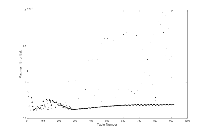
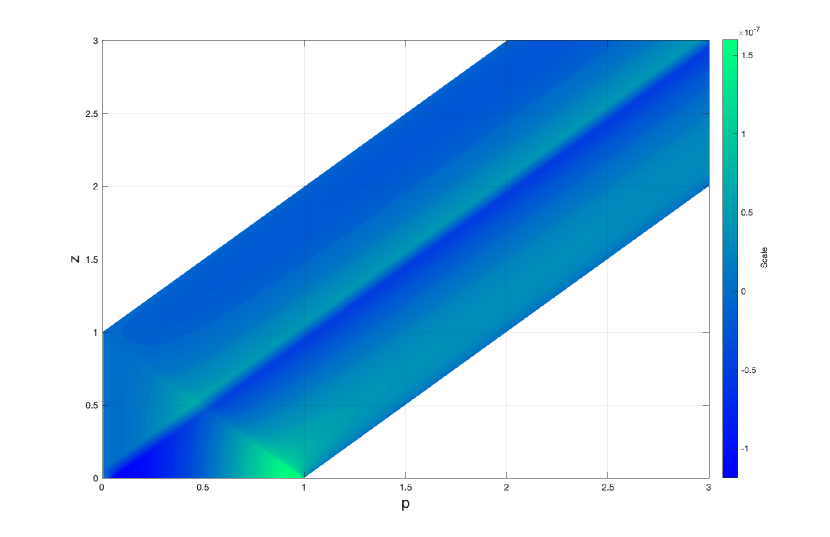
We now address the second question raised at the beginning of this section. Since the error induced by PL approximations is $O(\Delta x^{2})$, one would expect doubling the table size would reduce the error by a factor of 4. The approach to answering this question is to construct a much better table approximation than provided by a PL function. If we use the central difference approximation to the derivative of the intensity at each interior value of $\mu_{i}$, we obtain a second order approximation to $dI_{i}$. Thus we have the table $\big{[}\mu_{i},I_{i},dI_{i}\big{]}$ which defines a PCH function approximation of $I$. Rather than connecting the intensity values with line segments, where each adjacent pair is now connected by a cubic polynomial such that the PCH function is a continuous differentiable function for all values of $\mu$. For each of the 918 Neilson & Lester (2013) tables using the $Kepler$ band, we compute the maximum light curve difference between the PL and the PCH function approximations for the region in the $(p,z)$ plane given by $0<p<3$ and $0<z<3$. Figure 27 shows the maximum light curve error generated by the PL function defined by a table size $N_{\mu}=1001$ for all of the 918 models in the Neilson & Lester (2013) grid. The maximum error estimate is $2.1\times 10^{-7}$. The mean and median values from the grid are $7.15\times 10^{-8}$ and $6.79\times 10^{-8}$, respectively. Figure 28 shows a specific example, where we consider the Neilson & Lester (2013) table for $T_{\rm eff}=5700,~{}\log(g)=4.50$, and mass $M=1.1M_{\odot}$.

Table 1: Error Statistics

$T$	$N_{\mu}$	maximum	median
		difference	difference
1	1001	$2.143\times 10^{-6}$	$4.510\times 10^{-7}$
2	1001	$3.806\times 10^{-7}$	$4.248\times 10^{-8}$
4	1001	$7.356\times 10^{-8}$	$1.443\times 10^{-8}$
8	1001	$7.356\times 10^{-8}$	$1.209\times 10^{-8}$
1	2001	$2.145\times 10^{-6}$	$4.434\times 10^{-7}$
2	2001	$3.837\times 10^{-7}$	$2.968\times 10^{-8}$
4	2001	$6.762\times 10^{-8}$	$4.817\times 10^{-9}$
8	2001	$1.839\times 10^{-8}$	$3.089\times 10^{-9}$
1	4001	$2.145\times 10^{-6}$	$4.415\times 10^{-7}$
2	4001	$3.845\times 10^{-7}$	$2.709\times 10^{-8}$
4	4001	$6.803\times 10^{-8}$	$2.001\times 10^{-9}$
8	4001	$1.205\times 10^{-8}$	$8.694\times 10^{-10}$
1	8001	$2.145\times 10^{-6}$	$4.410\times 10^{-7}$
2	8001	$3.846\times 10^{-7}$	$2.645\times 10^{-8}$
4	8001	$6.813\times 10^{-8}$	$1.132\times 10^{-9}$
8	8001	$1.023\times 10^{-8}$	$3.019\times 10^{-10}$

Figure 1: An overview of the method described in this work. The starting point is a Table of $\mu$ with the corresponding intensity values. Such a table may be generated by a stellar atmosphere model or by a parametrized analytic limb darkening law. This $(\mu,I)$ table then generates a piecewise cubic Hermite function (PCHF), $G(r^{2})$, from Equation 7, and another PCHF $G(r^{2})/r^{2}$. These PCHFs are created without error. The dotted arrow going back to the original table, indicates that the original table can be recreated without loss from the PCHF $G(r^{2})/r^{2}$. Equation 4 gives the path integrals and equation 6 gives the 1-form $\big{[}P,Q\big{]}$. Hence, the PCHF $G(r^{2})/r^{2}$ is the desired form for the atmosphere table. This form directly generates the integrands of the path integral. The dark arrows indicate comparisons with the standard limb darkening laws assuming a table size of 1001 equally spaced values of $\mu$ in $[0,1]$.

Figure 2: The normalized intensity vs $\mu$ for the Spherical Model Stellar Atmosphere Table from Neilson & Lester (2013) for the stellar parameters $T_{\rm eff}=5700K$, $\log(g)=4.50$ and Mass=$1.1M_{\odot}$ in the $Kepler$ band.

Figure 3: The normalized intensity vs $r^{2}$ for the Spherical Model Stellar Atmosphere Table from Neilson & Lester (2013) for the stellar parameters $T_{\rm eff}=5700K$, $\log(g)=4.50$ and Mass=$1.1M_{\odot}$ in the $Kepler$ band.

Figure 4: $G(r^{2})$ vs $r^{2}$ for the Spherical Model Stellar Atmosphere Table from Neilson & Lester (2013) for the stellar parameters $T_{\rm eff}=5700K$, $\log(g)=4.50$ and Mass=$1.1M_{\odot}$ in the $Kepler$ band.

Figure 5: $G(r^{2})/r^{2}$ vs $r^{2}$ for the Spherical Model Stellar Atmosphere Table from Neilson & Lester (2013) for the stellar parameters $T_{\rm eff}=5700K$, $\log(g)=4.50$ and Mass=$1.1M_{\odot}$ in the $Kepler$ band.

Figure 6: Normalized intensity vs $r^{2}$ for the QL’s Linear Basis Function $I=\mu(r^{2})$.

Figure 7: The difference between the QL Linear Basis Function’s analytic form for $G(r^{2})/r^{2}$ and the Atmosphere form of $G_{\rm PCH}(r^{2})/r^{2}$ . The table sizes are denoted by blue=101, black=1001, and red=10001.

Figure 8: Normalized intensity vs $r^{2}$ for the QL’s Quadratic Basis function $I=\mu^{2}(r^{2})$.

Figure 9: The maximum error (black symbols) and the median error (red symbols) in the flux fraction in the $(p,z)$ plane as a function of the table length $N_{\mu}$, where $p$ is the ratio of the radii and $z$ is the distance between the centers in units of the radius of the back body. The triangles are for the QL, the circles are for the log law, and the stars are for the square root law.

Figure 10: The error in the flux fraction in the $(p,z)$ plane, where $p$ is the ratio of the radii and $z$ is the distance between the centers in units of the radius of the back body. This map was made using $T_{\rm ATM}=2$ and a table length of $N_{\mu}=1001$.

Figure 11: The frequency distributions for the errors in the computation of the flux fractions for various values of $T_{\rm ATM}$ with a table length of $N_{\mu}=1001$.

Figure 12: The frequency distributions for the errors in the computation of the flux fractions for various values of $N_{\mu}$ with a tolerance of $T_{\rm ATM}=4$.

Figure 13: Top: The time in $\mu$s needed to compute a flux fraction as a function of the radius ratio $p$. The black curve is for the occultquad routine from MA2002, and the blue curve is for the method of ${\rm Paper~{}I}$, using T$=2$. The green curves are for the new method with $T_{\rm ATM}=1$, 2, 3, 4, and 5. Bottom: The ratio of times relative to the MA2002 occultquad routine for $T_{\rm ATM}=1$ (blue) and $T_{\rm ATM=2}$ (red).

Figure 14: As described in Section 7, there are 101 model transits light curves, each with the same stellar and planet radius constructed using the ATM. The impact parameters of these models range from 0 to 1 in equal steps. Treating them as “data”, each of these light curves was fitted using the code described in ${\rm Paper~{}I}$, with the analytic quad law. The fitting was done for four parameters, namely the two quad-law coefficients, the planet’s radius, and the planet’s orbital inclination. The 101 residual light curves are shown here stacked, where the color represents the size of the difference between the flux from the analytic fitting and that from the ATM. Blue represents a positive difference while red represents a negative difference. The lowest horizontal line represents the impact parameter for which the planet rim makes contact with the center of the star. The middle line represents the impact parameter for which the planet’s rim makes contact with the inside of the stellar rim. The top line represents the parameter for which the planet’s center makes contact with the stellar rim.

Figure 15: The same construction as in Figure 14 but for the spectral B band.

Figure 16: The same construction as in Figure 14 but for the spectral H band.

Figure 17: The quad law coefficients $q_{1}$ (solid lines) and $q_{2}$ (dashed lines) derived from the fits in Figures 14, 15, and 16 are shown in the left panel as a function of the impact paramter where the colors represent the spectral bands, Kepler (green), B (blue), and H (red). The middle panel shows the relative error in the radius, and the right hand panel shows the relative error in the inclination.

Figure 18: The same construction as in Figure 14 but using the Power-2 law for the analytic model. The residuals for the Kepler spectral band are shown.

Figure 19: The same construction, for the Power-2 law, as in Figure 18 but for the B spectral band.

Figure 20: The same construction, for the Power-2 law, as in Figure 18 but for the H spectral band.

Figure 21: Similar to Figure 17, but using the Power-2 law in the analytic model. Here, the left panel shows the optimal Maxted Power-2 Law coefficients, $h_{1}$ (solid lines), and $h_{2}$ (dashed lines). Since the first coefficient is defined as the value of the intensity at $\mu=0.5$, it has a very small variation with the impact parameter and with the optimization. (See also our discussion of these coefficients in Short et al. 2019.)

Figure 22: Similar to Figure 17, but using the 4-parameter (“Claret”) law in the analytic model. The colors in the middle and right panels represent the spectral bands as before. The left panel shows the optimized coefficients for the Kepler band only: $c_{1}$ (black), $c_{2}$ (blue), $c_{3}$ (green), and $c_{4}$ (red).

Figure 23: Top: the change in the effective rotational radial velocity (R-M Effect) for the Hot Jupiter example with an impact parameter of 0.25 and using an inclination of $89.2545^{\circ}$, Rotation Period of 20 days, $\Phi_{\rm rot}=90^{\circ}$ , and a $\Theta_{\rm rot}=0^{\circ}$. Bottom: color represents the effective rotational radial velocity field on the star scaled by the color bar. The black circle is the limb of the transiting planet and the black line is the orbital track of the planet across the POS view of the star. $N$ is the north pole of the right handed stellar rotation axis.

Figure 24: Similar to Figure 23 but with a misaligned rotation axis given by $\Phi_{\rm rot}=30^{\circ}$, and $\Theta_{\rm rot}=-80^{\circ}$.

Figure 25: Histogram of the $\max_{\rm p~{}and~{}q}|F_{U}(p,z)|$ computed for 10,000 sample error tables using the unit normal distribution over the range in the $(p,z)$ plane given by $0<p<3$ and $0<z<3$.

Figure 26: Histogram of the $\max_{\rm pandq}|F_{U}(p,z)|$ computed for 10,000 sample error tables using the unit uniform distribution over the range in the $(p,z)$ plane given by $0<p<3$ and $0<z<3$.

Figure 27: The maximum difference between the PL and PCH function approximations computed over in the region $0<p<3$ and $0<z<3$ in the $(p,z)$ plane for each of the 918 models in the Neilson & Lester (2013) grid is shown. The model file t7500g475m5 was omitted from the analysis since it was an outlier.

Figure 28: Error estimate in the $(p,z)$ plane for the Neilson & Lester (2013) table for $T_{\rm eff}=5700,~{}\log(g)=4.50$, and mass $M=1.1M_{\odot}$.

References

- Agol et al. (2019) Agol, E., Luger, R., & Foreman-Mackey, D. 2020, AJ, 159, 123
- Aufdenberg, Ludwig & Kervella (2005) Aufdenberg, J. P., Ludwig, H. G., & Kervella, P. 2005, ApJ, 633, 424
- Beichman et al (2014) Beichman, C., Benneke, B., Knutson, H., et al. 2014, PASP, 126, 113
- Bitner & Robinson (2006) Bitner, M. A. & Robinson, E.L. 2006, ApJ, 131, 1712
- Claret (2000) Claret, A. 2000, A&A, 363, 1081
- Czesla et al. (2015) Czesla, S., Klocová, T., Khalafinejad, S., et al. 2015 A&A, 582, A51
- Diaz-Cordovez & Gimenez (1992) Diaz-Cordovez J., & Giménez, A. 1992, A&A, 259, 227
- ESA-PLATO (2017) ESA-SCI 2017 PLATO Definition Study Report ESA-SCI(2017)1, ESA-SCI
- Espinoza & Jordán (2015) Espinoza, N., & Jordán, A. 2015, MNRAS, 450, 1879
- Espinoza & Jordán (2016) Espinoza, N., & Jordán, A. 2016, MNRAS, 457, 3573
- Esteves et al. (2015) Esteves, L.J., De Mooij, E.J.W., & Jayawardhana, R. 2015, ApJ, 804, 150
- Gilliland et al (2011) Gilliland, R., Chaplin, W. J., Dunham, E. W., et al. 2011, ApJS, 197, 6
- Giménez (2006a) Giménez, A. 2006a, A&A, 450, 1231
- Hauschildt et al. (1999) Hauschildt, P. H., Allard, F., Ferguson, J., Baron, E., & Alexander, D. R. 1999, ApJ, 525, 871
- Hayek et al. (2012) Hayek, W., Sing, D., Pont, F., & Asplund, M. 2012, A&A, 539, A102
- Heller (2019) Heller, R. 2019, A&A, 623, A137
- Hestroffer (1997) Hestroffer, D. 1997, A&A, 327, 199
- Hill (1979) Hill, G. 1979, PDAO, 15, 297
- Hill & Rucinski (1993) Hill, G., & Rucinski, S. M. 1993, in IAU Symp. 151, Light Curve Modeling of Eclipsing Binary Stars, ed. E. F. Malone (New York: Springer), 135
- Hosokawa (1953) Hosokawa, Y. 1953, PASJ, 5, 88
- Howarth (2011) Howarth, I. D. 2011, MNRAS, 418, 1165
- Kipping & Bakos (2011a) Kipping, D., & Bakos, G. 2011a, ApJ, 730, 50
- Kipping & Bakos (2011b) Kipping, D., & Bakos, G. 2011b, ApJ, 733, 36
- Kipping (2013) Kipping, D. M. 2013, MNRAS, 435, 2152
- Klinglesmith & Sobeiski (1970) Klinglesmith, D. A., & Sobeiski, S. 1970, AJ, 75, 175
- Kopal (1950) Kopal, Z. 1950, HarCi, 454, 1
- Lester & Neilson (2008) Lester, J. B., & Neilson, H. R. 2008, A&A, 491, 633
- Linnell & DeStefano (2012) Linnell, A. P., DeStefano, P., & Hubeny, I. 2012, PASP, 124, 885
- Linnell et al. (2013) Linnell, A. P., DeStefano, P., & Hubeny, I. 2013, AJ, 146, 68
- Linnell & Hubeny (1994) Linnell, A. P., & Hubeny, I. 1994, ApJ, 434, 738
- Magic et al. (2015) Magic, Z., Chiavassa, A., Collet, R., & Asplund, M. 2015, A&A, 573, A90
- Magic et al. (2013) Magic, Z., Collet, R., Asplund, M., et al. 2013, A&A, 557, A26
- Mandel & Agol (2002) Mandel, K., & Agol, E. 2002, ApJ, 580, 171
- Maxted (2018) Maxted, P. F. L. 2018, A&A, 616, A39
- Milne (1923) Milne, E. A. 1923, RSPTA, 223, 201
- Milne (1930) Milne, E. A. 1930, HDA, 3, 65
- Morello et al. (2020) Morello, G., Claret, A., Martin-Lagarde, M., et al. 2020, AJ, 159,75
- Morello et al (2017) Morello, G., Tsiaras, A., Howarth, I. D., & Homeier, D. 2017, AJ, 154, 111
- Neckel & Labs (1994) Neckel, H., & Labs, D. 1994, Sol. Phys., 153, 91
- Neilson & Lester (2013) Neilson, H. R., & Lester, J. B. 2013, A&A, 556, A86
- Neilson (2019) Neilson, H.R., Lester, J.B., & Baron, F. 2018, arXiv:1805.02696
- Neilson et al. (2017) Neilson, H. R., McNeil, J. T., Ignace. R., & Lester, J. B. 2017, ApJ, 845, 65
- Orosz & Hauschildt (2000) Orosz, J. A., & Hauschildt, P. H. 2000, A&A, 364, 265
- Pál (2012) Pál, A. 2012, MNRAS, 420, 1630
- Pettit (1939) Pettit, E. 1939 PASP, 51, 321
- Prša & Zwitter (2005) Prša, A., & Zwitter, T. 2005, ApJ, 628, 426
- Prsa et al. (2016) Prša, A., Conroy, K. E., Horvat, M., 2016, ApJS, 227, 29
- Przybylski (1957) Przybylski, A. 1957, MNRAS, 117, 600
- Schwarzschild (1906) Schwarzschild, K. 1906, WisGo, 195 41
- Short (2019) Short, D. R., 2019 Matlab Demonstration Code for the Calculation of Flux Fraction and the Rossiter-Mclaughlin Effect using ATM data, v1.0, Zenodo, doi: 10.5281/zenodo.3473851
- Short et al. (2018) Short, D. R., Orosz, J. A., Windmiller, G., & Welsh, W. F. 2018, AJ, 156, 297
- Short et al. (2019) Short, D. R., Welsh, W. F., Orosz, J. A., Windmiller, G., & Maxted, P. F. L. 2019 RNAAS, 3, 117
- Skilling (2006) Skilling, J. 2006, BayAn, 1, 833
- Tinetti (2016) Tinetti, G., Drossart, P., Eccleston, P., et al. 2016 Proc. SPIE, 9904E, 1
- Willson & Devinney (1971) Wilson, R. E., & Devinney, E. J. 1971, ApJ, 166, 605
- Wittenmyer et al. (2005) Wittenmyer, R. A., Welsh, W. F., Orosz, J. A., et al. 2005, ApJ, 632, 1157
- Yan et al. (2017) Yan, F., Pallé, E., Fosbury, R. A. E., Petr-Gotzens, M. G., & Henning, Th. 2017 A&A, 603, A73