Measuring the masses of magnetic white dwarfs: A NuSTAR Legacy Survey

Abstract

The hard X-ray spectrum of magnetic cataclysmic variables can be modelled to provide a measurement of white dwarf mass. This method is complementary to radial velocity measurements, which depend on the (typically rather uncertain) binary inclination. Here we present results from a Legacy Survey of 19 magnetic cataclysmic variables with NuSTAR. We fit accretion column models to their 20–78 keV spectra and derive the white dwarf masses, finding a weighted average $\bar{M}_{\rm WD}=0.77\pm 0.02$ $M_{\odot}$, with a standard deviation $\sigma=0.10$ $M_{\odot}$, when we include the masses derived from previous NuSTAR observations of seven additional magnetic cataclysmic variables. We find that the mass distribution of accreting magnetic white dwarfs is consistent with that of white dwarfs in non-magnetic cataclysmic variables. Both peak at a higher mass than the distributions of isolated white dwarfs and post-common-envelope binaries. We speculate as to why this might be the case, proposing that consequential angular momentum losses may play a role in accreting magnetic white dwarfs and/or that our knowledge of how the white dwarf mass changes over accretion–nova cycles may also be incomplete.

1 Introduction

Cataclysmic Variables (CVs) are binary systems in which a white dwarf (WD) accretes matter from a stellar companion via Roche lobe overflow (for an in-depth review of CVs see Warner, 2003). Magnetic CVs (mCVs) are a class of CVs in which the central WD has a strong magnetic field ($B\sim 10^{6}-10^{8}$G), which disrupts the accretion disc and forces the accreted material to travel along the magnetic field lines on to the WD poles (see reviews by Cropper, 1990; Patterson, 1994). Depending on the strength of the magnetic field, mCVs can be further divided into two subclasses. In Intermediate Polars (IPs), only the innermost regions of the disc are disrupted, typically leaving a residual outer disc which terminates at the magnetospheric radius ($R_{\rm m}$). It is at this point where matter begins to flow along the magnetic field lines in so-called ‘accretion curtains.’ In polars, the magnetic field of the WD is strong enough such that matter flows along the field lines from the donor without forming a disc.

Aside from the differing magnetic field strengths, polars and IPs can be observationally differentiated by the ratio of the WD spin period ($P_{\rm spin}$) to the binary orbital period ($P_{\rm orb}$). In polars, $P_{\rm spin}=P_{\rm orb}$, but in IPs $P_{\rm spin}<P_{\rm orb}$, usually $<<P_{\rm orb}$ (see e.g. Patterson, 1994; Hellier, 2014). There are a small number of so-called ‘asynchronous’ polars (APs) which exhibit the same properties as regular polars, but $P_{\rm spin}$ and $P_{\rm orb}$ differ by a factor of $\sim 1$% (see e.g. Schmidt & Stockman, 1991; Littlefield et al., 2015).

Regardless of their subclass, mCVs are strong X-ray emitters (see Mukai, 2017, for a review). Close to the surface of the WD, the in-falling material forms a standing shock, with typical temperatures of $kT\gtrsim 10$ keV (Aizu, 1973). As the gas in the post-shock region descends on to the surface of the WD and cools, it emits hard X-rays via optically thin thermal emission. It has been shown that the shock temperature is directly linked to the compactness of the WD (Katz, 1977; Rothschild et al., 1981). Thus, measuring the spectral turnover via hard X-ray spectroscopy of mCVs can be used to derive accurate WD masses. X-ray spectroscopy provides a method of measuring WD mass independent of radial velocity studies, which are often dominated by uncertainties in binary inclination (Suleimanov et al., 2005; Yuasa et al., 2010; Suleimanov et al., 2019). An alternative X-ray spectroscopic method compares the fluxes from Fe K lines of different ionization states, to measure the post-shock temperature (Fujimoto & Ishida, 1997; Ezuka & Ishida, 1999; Xu et al., 2019).

The derivation of WD mass is fundamental for quantative studies of individual objects. However, it is arguably even more important to know the WD mass distribution in order to understand the formation and evolution of CVs. The average mass of isolated WDs ($\sim 0.6M_{\odot}$; Kepler et al., 2016b) is known to be lower than that of non-magnetic CVs ($\sim 0.8M_{\odot}$; Zorotovic et al., 2011), though we note that for WDs within 100 pc, the mass distribution is apparently bimodal with peaks at 0.6 and 0.8 $M_{\odot}$ (Kilic et al., 2018). Furthermore, isolated magnetic WDs appear to be more massive on average ($\bar{M}_{\rm WD}=0.784\pm 0.047$ $M_{\odot}$; Ferrario et al., 2015) than their non-magnetized counterparts (see also fig. 12 of Ferrario et al., 2020).

In addition, comparing the WD mass distributions between non-magnetic and mCVs may be useful in testing theories of the origin of the magnetic field in WDs. A leading scenario for the single magnetic WDs is that they are the results of mergers during the common envelope phase; mCVs are then understood to be the consequence of close interaction during the common envelope phase that end just short of merger (see e.g. Ferrario et al. 2015 but cf. Belloni & Schreiber 2020). Such a scenario could feasibly lead to a measurable difference between the mean masses of magnetic and non-magnetic WDs in CVs. Conversely, if magnetic and non-magnetic CVs share similar mass distributions, then one must question the evolution of WD mass once a binary becomes a CV, regardless of magnetic field strength. For example, the idea that CVs undergo a period of mass growth through accretion contradicts a number of existing theories of nova eruptions, which suggest that the amount of ejected mass is larger than the amount accreted (e.g. Prialnik & Kovetz, 1995; Yaron et al., 2005; Hillman et al., 2020).

Early (pre-2000) X-ray studies of WD masses in mCVs were limited to energies $\lesssim 20$ keV that were probed by the X-ray observatories of the time (e.g. Cropper et al., 1998; Cropper et al., 1999). The uncertainties were large, owing to the spectral cutoff (which is essential for mass determination) in mCVs usually occurring beyond 20 keV. However, with the inclusion of sensitive hard X-ray instruments on board satellites such as the Rossi X-ray Timing Explorer (RXTE; Bradt et al., 1993), Neil Gehrels Swift Observatory (Swift; Gehrels et al., 2004), Suzaku (Mitsuda et al., 2007) and the International Gamma-Ray Astrophysics Laboratory (INTEGRAL; Winkler et al., 2003), mass measurements became more reliable and accurate. Studies with these instruments suggested that mCVs exhibit a similar mass distribution to that of their non-magnetic counterparts (see e.g. Suleimanov et al. 2005; Brunschweiger et al. 2009; Yuasa et al. 2010; Bernardini et al. 2012, as well as de Martino et al. 2020 and references therein for a review). Despite the improvement, these surveys still suffered from uncertain X-ray background (which must be modelled rather than extracted for non-imaging instruments such as Suzaku’s Hard X-ray Detector; Fukazawa et al., 2009).

However, the emergence of the Nuclear Spectroscopic Telescope Array (NuSTAR; Harrison et al., 2013) as the first telescope to be able to focus X-rays above 12 keV has brought about the ability to perform high angular-resolution imaging and spectroscopy in the hard X-ray regime. NuSTAR is therefore the ideal instrument to perform a systematic survey of mCVs in order to efficiently measure the mass distribution of magnetic WDs. Mass measurements of IPs have been made with NuSTAR previously (Hailey et al., 2016; Suleimanov et al., 2016; Shaw et al., 2018; Suleimanov et al., 2019), but have focused on a few sources at a time (for a total of 7 WD masses). In this work we present results from NuSTAR observations of an additional 19 mCVs as part of the NuSTAR Legacy Survey program.

1.1 Modelling mCV masses

The standing shock in mCVs heats the infalling gas, which then cools via optically thin thermal bremsstrahlung as it descends on to the surface of the WD. The hard X-ray continuum of mCVs, therefore, can be broadly modelled as a series of thermal bremsstrahlung components. However, the location of the shock, close to the WD surface, means that some X-ray emission will be directed towards the WD and reflected back towards the observer. Reflection modifies the underlying continuum with a Compton ‘hump’ at $\sim 10-30$ keV and neutral Fe-K emission at $6.4$ keV. When considering the whole NuSTAR energy band, reflection has been found to be very important in modeling the X-ray spectrum of mCVs (Mukai et al., 2015). Finally, the spectra of some mCVs may be affected by additional partial obscuration by the accretion curtains, even reaching the NuSTAR band (see e.g. Done & Magdziarz, 1998; Cropper et al., 1999; Shaw et al., 2018).

For the mCVs discussed in this work, we use the IP mass model derived by Suleimanov et al. (2016, 2019, see these works for in-depth discussion of the model), which calculates a WD mass ($M_{\rm WD}$) based on the temperature of the underlying continuum. We follow Suleimanov et al. (2019) and refer to this as the ‘PSR’ (post-shock region) model. $M_{\rm WD}$ is calculated assuming the Nauenberg (1972) mass-radius relation for cold WDs. The temperature of the shock, $kT_{\rm sh}$, depends on the velocity of infalling matter. Earlier models make the (often reasonable) assumption that the matter free-falls from infinity (e.g. Suleimanov et al., 2005; Yuasa et al., 2010). In reality, and particularly in the case of IPs, free-fall begins at $R_{\rm m}$, where the accretion disc terminates. $R_{\rm m}$ can be small enough in some cases that the accretion flow will reach a velocity substantially smaller than the escape velocity, leading to a lower value of $kT_{\rm sh}$. Assuming $R_{\rm m}$=$\infty$ in such cases would lead to an underestimation of the WD escape velocity, and thus of $M_{\rm WD}$. The PSR model therefore utilizes a two-parameter grid of hard X-ray spectra, with $M_{\rm WD}$ and $R_{\rm m}$ (relative to the WD radius, $R_{\rm WD}$) as free parameters. Suleimanov et al. (2019) introduced a slightly modified version of the model which also considers the height of the shock itself (as a shock height that is a significant fraction of the WD radius would also substantially reduce the escape velocity), but this only becomes important for sources with a low local mass-accretion rate ($\lesssim 1$ g s^-1 cm^-2). Given that the Legacy sample are all high luminosity ($L\gtrsim 10^{33}$ erg s^-1; see Suleimanov et al., 2019, see also Table 2), we can assume that they have high local mass accretion rates too. However, we do discuss the effect that the shock height has on derived mass in Section 3.4.3.

When applied to the hard X-ray spectrum of an mCV, the PSR model defines a curve in the $M_{\rm WD}$—$R_{\rm m}$ plane. One can then derive another curve in the same plane by measuring a break in the power spectrum of the source light curve. The concept here is that the accretion disk generates noise at frequencies related to the orbital frequency, so the power spectrum cuts off at high frequency, where the magnetosphere truncates the inner accretion disk. Revnivtsev et al. (2009, 2011) showed that the break frequency $\nu_{\rm b}$ corresponds to the Keplerian frequency at $R_{\rm m}$ according to

$$\nu_{\rm b}=\sqrt{\frac{GM_{\rm WD}}{2\pi R^{3}_{\rm m}}}.$$ (1)

The intersection of the two curves then allows us to derive $M_{\rm WD}$ and $R_{\rm m}$ (see Fig. 1 for an example for a Legacy survey target). Suleimanov et al. (2019) applied this technique to 5 IPs that exhibited power spectrum breaks, finding that $M_{\rm WD}$ only changes significantly if $R_{\rm m}\lesssim 4$ $R_{\rm WD}$, as in the cases of GK Per (in outburst) and EX Hya.

2 Observations and Analysis

Table 1: Summary of NuSTAR observations

Source	ObsID	Start Date/Time	MJDa	Exposure time
		(UTC)		(ks)
1RXS J052523.2$+$241331	30460020002	2019 Mar 21 13:31:09	58563.56	58.8
V515 And	30460019002	2019 Mar 09 20:51:09	58551.87	62.2
V1432 Aql∗	30460004002	2018 Apr 05 04:51:09	58213.20	27.2
FO Aqr	30460002002	2018 Apr 16 02:01:09	58224.08	25.6
V405 Aur	30460007002	2017 Nov 08 20:01:09	58065.83	38.3
BY Cam∗	30460010002	2018 Nov 12 15:21:09	58434.64	33.0
BG CMi	30460018002	2018 Oct 09 19:46:09	58400.82	40.4
V2069 Cyg	30460023002	2019 Jun 27 23:46:09	58661.99	67.4
PQ Gem	30460009002	2019 Mar 27 14:36:09	58569.61	42.0
V2400 Oph	30460003002	2019 Mar 07 18:31:09	58549.77	27.0
AO Psc	30460008002	2018 Jun 29 04:21:09	58298.18	37.4
V667 Pup	30460012002	2019 May 20 21:36:09	58623.90	39.4
V1062 Tau	30460015002	2020 Mar 17 01:31:09	58925.06	31.5
…	30460015004	2020 Mar 17 18:31:49	58925.77	30.4
EI UMa	30460011002	2019 Mar 20 18:21:09	58562.76	35.0
IGR J08390$-$4833	30460025002	2018 Feb 09 08:01:09	58158.33	55.2
IGR J15094$-$6649	30460013002	2018 Jul 19 23:01:09	58318.96	41.3
IGR J16547$-$1916	30460016002	2019 Mar 16 05:16:09	58558.22	44.6
IGR J17195$-$4100	30460005002	2018 Oct 25 22:56:09	58416.96	29.5
RX J2133.7$+$5107	30460001002	2018 Feb 23 12:51:09	58172.54	26.2

^∗Asynchronous Polar
^a MJD at the start of the observation

In this work we utilize observations of 17 IPs and two APs from the NuSTAR Legacy survey of mCVs, spanning a period of $\sim 2.5$yr. Individual targets, observation dates and their exposure times are detailed in Table 1. There were four additional targets, observed as part of the Legacy programme, that we do not include in the analysis for various reasons. IGR J14536$-$5522 is a polar that was not detected in a 46.0 ks NuSTAR observation, and was likely in a low state due to a reduced mass-accretion rate (commonly seen in polars; Ramsay et al., 2004). YY/DO Dra is an IP that was not detected in a 55.4 ks NuSTAR observation. Low states are much rarer in IPs than in polars (see e.g. Kennedy et al., 2017), but a Swift observation, quasi-simultaneous with NuSTAR, confirms the low state of YY/DO Dra. XY Ari is an IP that was observed by NuSTAR, but the observation was interrupted by a high priority target of opportunity observation and was never completed. The 9.3 ks of data that do exist are not enough to constrain a mass using the methodology we describe below. RX J2015.6$+$3711 is a CV of uncertain classification, but has been suggested to be an IP (Coti Zelati et al., 2016). A 59.6 ks NuSTAR observation does not allow us to constrain a mass using the methodology we describe below as the source is a factor $\sim 6$ fainter than the reported Swift/Burst Alert Telescope (BAT; Barthelmy et al., 2005) 70 month catalogue flux (Mukai, 2017), raising the possibility that, like DO Dra, RX J2015.6$+$3711 is also in a low state.

Three Legacy targets (FO Aqr, V405 Aur and RX J2133.7$+$5107) have been discussed by Suleimanov et al. (2019) alongside the 7 IPs previously observed with NuSTAR, but we re-reduce and analyse the data for those three in this study. We do not re-reduce the observations of the 7 previously observed IPs, instead choosing to combine our Legacy results with the published results from those sources (see Suleimanov et al., 2019, and references therein for detailed analyses of the non-Legacy data).

We reduced the data using the NuSTAR data analysis software (NuSTARDAS) v1.8.0 packaged with heasoft v6.26.1. The exception to this is the observation of V1062 Tau, which took place on 2020 March 17, and thus required NuSTARDAS v1.9.2 (packaged with heasoft v6.27.2) in order to account for the adjustment of NuSTAR’s onboard laser metrology system. Data taken prior to 2020 March 17 are unaffected by this change so reprocessing was not necessary.

We used the nupipeline task to perform standard data processing, including filtering for high levels of background during the telescope’s passage through the South Atlantic Anomaly and generation of exposure maps. We extracted spectra and (10s binned) light curves from the resultant cleaned event files (from both NuSTAR focal plane modules; FPMA and FPMB) using the nuproducts task. Source spectra and light curves were extracted from a circular region of radius ranging from $30-70$″. The background was typically extracted from a 70″circular region in the opposite corner of the same chip that the source lay on. However, the observation of the IP 1RXS J052523.2$+$241331 was badly affected by photons from a nearby source that bypassed the telescope optics ("stray light", Madsen et al., 2017). In both FPMs, the source fell on the region of the detector containing the stray light, and we extracted the background spectrum from a 50″region that included the stray light photons.

We grouped the spectra such that each spectral bin had a signal-to-noise ratio S/N=3 using the heasoft task grppha. Light curves from FPMA and FPMB were co-added with the heasoft tool lcmath and then corrected to the solar system barycentre with barycorr.

The break in IP power spectra discussed in Section 1.1 is easiest to detect if the periodic variability from WD spin is removed from the light curve first. To do this we followed a similar method as Suleimanov et al. (2019). We first split the NuSTAR light curve into segments, the number of which was dependent on the length of the light curve, the source count rate and the WD $P_{\rm spin}$. We folded each segment on the known $P_{\rm spin}$ from the literature. Using the same folding parameters, we calculated the pulse phase for each light curve segment time stamp and subtracted the expected rate from the observed rate. The power spectra of the resultant aperiodic light curves were then calculated using the stingray python library, a suite of tools dedicated to time series analysis (Huppenkothen et al., 2016; Huppenkothen et al., 2019). We note that the above analysis only applies to the 17 IPs in our sample, as the APs do not have a disc. We detect a break in only one of our sample, FO  Aqr at $\nu_{\rm b}=1.3\times 10^{-3}$ Hz, confirming the findings of Suleimanov et al. (2019). For this source we used the tool flx2xsp to convert the aperiodic power spectrum into a format readable by the X-ray spectral fitting package xspec (Arnaud, 1996). It is important to note that the non-detection of a break in the power spectra of our target IPs does not have strong implications for the derived $M_{\rm WD}$. The bottom panel of Fig. 1 shows that $M_{\rm WD}$ is insensitive to changes in $R_{\rm m}$ unless it is very close ($\lesssim 4$$R_{\rm WD}$) to the WD, in which case $M_{\rm WD}$ would increase. We might expect this in sources with a higher than typical mass accretion rate due to e.g. a dwarf nova outburst, where the magnetosphere is compressed (see e.g. Suleimanov et al., 2019, and their discussion of GK Per), but not for the majority of IPs.

To derive $M_{\rm WD}$ for each source, we fit its X-ray spectrum with the Suleimanov et al. (2019) PSR model. As discussed in Section 1.1, the X-ray spectrum of mCVs is often complicated by the presence of a combination of partial covering and reflection components. When considering the whole NuSTAR band (3–78 keV), the derivation of $M_{\rm WD}$ then relies heavily on the choice of reflection and absorption models to account for these effects, and no robust description of both such components exists in the context of mCVs (see discussions by Suleimanov et al., 2016, 2019). Furthermore, in the PSR model, $M_{\rm WD}$ is mostly driven by the turnover of the spectrum at high energies. We therefore choose to restrict our fitted energy range to 20–78 keV in order to minimize the contributions from reflection and partial covering effects to the overall spectrum. This is not an unusual approach (see discussions by e.g. Suleimanov et al., 2016; Hailey et al., 2016; Suleimanov et al., 2019), and it allows us to derive $M_{\rm WD}$ without having to consider the multitude of complex effects that dominate the X-ray spectrum below 20 keV. There is one exception: for 1RXS J052523.2$+$241331, we instead restricted the fit to 20–50 keV, to minimize the contribution by stray light photons, which dominate the spectrum beyond $>50$ keV.

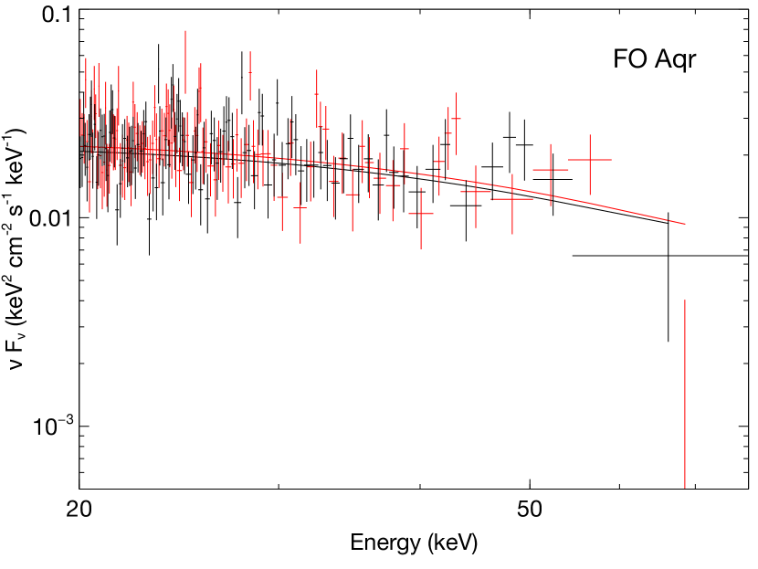
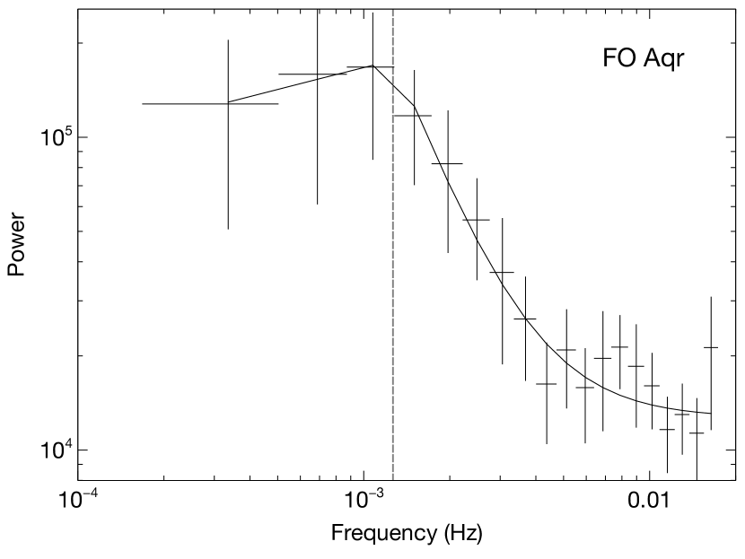
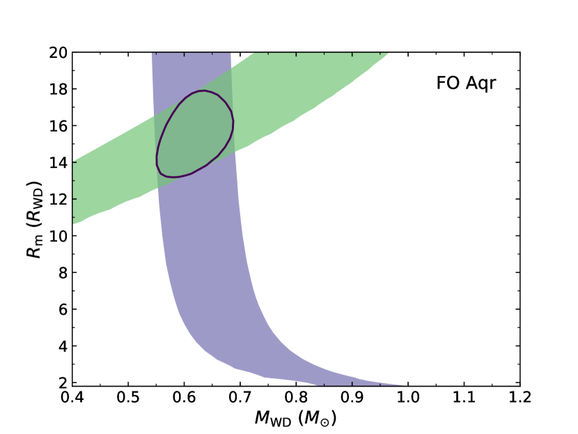
Figure 1: Upper Panel: NuSTAR FPMA (black) and FPMB (red) spectra of FO Aqr, fit with the Suleimanov et al. (2019) PSR model and plotted unfolded in $\nu$F_ν space. Middle Panel: Aperiodic power spectrum of the NuSTAR light curve of FO Aqr, fit with a broken power law. The power spectrum shows a break at $\nu_{\rm b}=1.3\times 10^{-3}$ Hz (indicated by the vertical dashed line), which can be linked to the $R_{\rm m}$ and $M_{\rm WD}$ parameters in the (energy) spectral model in xspec. Lower Panel: 90% confidence contours in the $M_{\rm WD}$—$R_{\rm m}$ plane calculated by fitting the power spectrum (green) and the energy spectrum (purple) separately. The solid closed curve represents the 90% confidence region obtained by fitting the power and energy spectra together. The best-fit parameters for FO Aqr are presented in Table 2.

For the unique case of FO Aqr, where we detect a break in the power spectrum, we are able to link the break frequency to the $R_{\rm m}$ parameter in the model using Equation 1 and fit the energy and power spectra simultaneously (see Fig. 1). For the other IPs, we assume that the WD is close to spin equilibrium; that is, that accreting matter has the same angular velocity as the WD. If this is not the case, there will be a torque trying to slow or speed the WD’s rotation. For IPs that have accreted persistently for a long time, we may assume that the WD has come into spin equilibrium (see e.g. Patterson et al., 2020). In this case, the Keplerian velocity of accreting material at $R_{\rm m}$ will match the WD’s spin;

$$R_{\rm m}\simeq R_{\rm co}=\left(\frac{GM_{\rm WD}P^{2}_{\rm spin}}{4\pi^{2}}\right)$$ (2)

where $R_{\rm co}$ is the corotation radius. This is a reasonable assumption for all the IPs in our sample, which are persistent sources that show no signs of transient outbursts in public all-sky monitoring data from the Swift/BAT and Monitor of All-Sky X-ray Image (MAXI; Matsuoka et al., 2009).

To include the spin equilibrium assumption in our xspec spectral fits, we set the $R_{\rm m}$ parameter to be a function of the $M_{\rm WD}$ parameter using Equation 2. For the APs, we assume $R_{\rm m}=1000R_{\rm WD}$, which is equivalent to $R_{\rm m}=\infty$ in the xspec model. For all observations, we fit the FPMA & FBMB spectra simultaneously, with the cross-normalisation between the two instruments accounted for by a constant. All xspec fits utilised $\chi^{2}$ as the fitting statistic, and all uncertainties presented in this work are given at $90\%$ confidence unless otherwise stated.

3 Results and Discussion

Table 2: Results of the NuSTAR Legacy Survey. The values of $R_{\rm m}$ and $M_{\rm WD}$ are extracted from the best-fit PSR model and $kT_{\rm bremss}$ is extracted from a single temperature bremmstrahlung fit to the spectra (bremss in xspec) and is not intended to be a full treatment of the shock temperature (see e.g. Mukai et al., 2015).

Source	$R_{\rm m}$	$M_{\rm WD}$	$kT_{\rm bremss}$	$F^{a}$	$d^{b}$	$L^{c}$
	($R_{\rm WD}$)	($M_{\odot}$)	(keV)	($10^{-10}$ erg cm-2 s-1)	(pc)	($10^{33}$ erg s-1)
1RXS J052523.2+241331d	$7.4^{*}$	$0.81^{+0.13}_{-0.10}$	$19.6^{+5.2}_{-3.6}$	$0.55^{+0.09}_{-0.07}$	$1888^{+363}_{-266}$	$23.5^{+9.9}_{-7.2}$
V515 And	$10.7^{*}$	$0.73\pm 0.06$	$18.2^{+2.3}_{-2.0}$	$0.70^{+0.08}_{-0.06}$	$978^{+46}_{-42}$	$8.0^{+0.12}_{-0.10}$
V1432 Aql	$\infty^{\dagger}$	$0.76^{+0.09}_{-0.08}$	$20.8^{+3.9}_{-3.1}$	$0.85^{+0.12}_{-0.09}$	$456^{+10}_{-9}$	$2.1^{+0.3}_{-0.2}$
FO  Aqr	$15.0^{+2.1}_{-1.5}$	$0.61^{+0.06}_{-0.05}$	$14.8^{+1.8}_{-1.7}$	$1.41^{+0.20}_{-0.17}$	$518^{+14}_{-13}$	$4.5^{+0.7}_{-0.6}$
V405 Aur	$12.3^{*}$	$0.75^{+0.07}_{-0.06}$	$19.1^{2.6}_{-2.2}$	$0.95^{+0.11}_{-0.09}$	$662^{+14}_{-13}$	$5.0^{+0.6}_{-0.5}$
BY Cam	$\infty^{\dagger}$	$0.76\pm 0.06$	$21.0^{+2.4}_{-2.0}$	$1.49^{+0.13}_{-0.11}$	$270\pm 2$	$1.3\pm 0.1$
BG CMi	$18.2^{*}$	$0.78^{+0.08}_{-0.07}$	$20.7^{+3.1}_{-2.6}$	$0.74^{+0.09}_{-0.07}$	$966^{+55}_{-50}$	$8.3^{+1.3}_{-1.2}$
V2069 Cyg	$14.7^{*}$	$0.73^{+0.09}_{-0.08}$	$18.5^{+2.8}_{-3.6}$	$0.46^{+0.07}_{-0.06}$	$1140^{+43}_{-40}$	$7.2^{+1.3}_{-1.0}$
PQ Gem	$15.3^{*}$	$0.71^{+0.06}_{-0.05}$	$18.0^{+2.3}_{-1.9}$	$0.94^{+0.11}_{-0.09}$	$750^{+21}_{-20}$	$6.3^{+0.8}_{-0.7}$
V2400 Oph	$15.5^{*}$	$0.67^{+0.06}_{-0.05}$	$16.6^{+2.0}_{-1.7}$	$1.59^{+0.19}_{-0.16}$	$701^{+17}_{-16}$	$9.3^{+1.2}_{-1.0}$
AO Psc	$11.6^{*}$	$0.55\pm 0.05$	$12.4^{+1.7}_{-1.4}$	$1.48^{+0.28}_{-0.22}$	$488^{+11}_{-10}$	$4.2^{+0.8}_{-0.6}$
V667 Pup	$13.4^{*}$	$0.83^{+0.11}_{-0.08}$	$22.8^{+4.3}_{-3.4}$	$0.63^{+0.07}_{-0.06}$	$798^{+51}_{-46}$	$5.1^{+0.9}_{-0.8}$
V1062 Tau	$43.0^{*}$	$0.72^{+0.07}_{-0.06}$	$18.7^{+2.4}_{-2.0}$	$0.71^{+0.08}_{-0.07}$	$1512^{+209}_{-165}$	$19.5^{+5.8}_{-4.7}$
EI UMa	$19.4^{*}$	$0.91^{+0.15}_{-0.13}$	$26.0^{+8.1}_{-5.6}$	$0.39^{+0.06}_{-0.05}$	$1095^{+47}_{-43}$	$5.6^{+1.0}_{-0.8}$
IGR J08390$-$4833	$26.4^{*}$	$0.81^{+0.13}_{-0.11}$	$12.1^{+5.8}_{4.2}$	$0.30^{+0.05}_{-0.04}$	$2064^{+311}_{-240}$	$15.4^{+5.4}_{-4.1}$
IGR J15094$-$6649	$15.4^{*}$	$0.73\pm 0.06$	$18.5^{+2.4}_{-2.0}$	$0.97^{+0.11}_{-0.09}$	$1127^{+37}_{-35}$	$14.8^{+1.9}_{-1.7}$
IGR J16547$-$1916	$12.2^{*}$	$0.74^{+0.09}_{-0.08}$	$18.9^{+3.4}_{-2.7}$	$0.58^{+0.09}_{-0.07}$	$1066^{+61}_{-54}$	$7.8^{+1.5}_{-1.2}$
IGR J17195$-$4100	$21.8^{*}$	$0.84^{+0.08}_{-0.07}$	$22.9^{+3.6}_{-2.9}$	$0.97^{+0.10}_{-0.08}$	$643^{+17}_{-16}$	$4.8^{+0.6}_{-0.5}$
RX J2133.7+5107	$17.5^{*}$	$0.96^{+0.08}_{-0.07}$	$28.2^{+4.6}_{-3.7}$	$1.06^{+0.08}_{-0.07}$	$1325^{+48}_{-45}$	$22.2^{+2.4}_{-2.2}$

^a Best-fit model flux (unabsorbed) from the PSR model in the 0.1–100 keV range, calculated using the cflux model in xspec (we choose this range for easy comparisons with Suleimanov et al. (2019))
^b Distance from Gaia DR2 (Bailer-Jones et al., 2018)
^c Luminosity calculated from best-fit model flux of the PSR model in 0.1–100 keV range
^dSpectrum was fit in the 20–50 keV range due to stray light
^∗ $R_{\rm m}=R_{\rm co}$ assumed
^† $R_{\rm m}=1000R_{\rm WD}$ assumed in xspec

3.1 Comparisons with other WD distributions

The measured masses from our 19 Legacy targets are listed in Table 2 and the spectra are plotted for reference in Fig. 6. For the Legacy sample, we calculate a weighted average $\bar{M}_{\rm WD}=0.72$, which increases to $\bar{M}_{\rm WD}=0.77$ if we include the 7 IPs previously observed with NuSTAR (Suleimanov et al., 2019). We refer to the Legacy+Suleimanov et al. (2019) sample as the "full NuSTAR sample." To estimate uncertainties on $\bar{M}_{\rm WD}$, we first calculate the standard deviation of the sample around the weighted average and find $\sigma=0.09$ $M_{\odot}$ ($\sigma=0.10$ $M_{\odot}$) for the Legacy (full NuSTAR) samples. In both cases, this value is larger than what is implied by the numerical error in the weighted mean (0.01 and 0.006 $M_{\odot}$, respectively) after correcting for the population size. This can occur if the errors of individual data points are underestimated. To quantitatively address this, we calculated 10000 weighted averages from a randomly selected sample of the Legacy only, or Legacy+Suleimanov et al. (2019) mCVs (bootstrap-with-replacement) and measured the 68% confidence interval. We find this to be $0.02$ $M_{\odot}$ for both the Legacy and full NuSTAR samples. The correction of this for population size agrees with the calculated values of $\sigma$ above. Since the mean of the 10000 bootstrapped weighted averages agrees with the weighted average of the full sample, we find no evidence of bias in our masses. We thus quote weighted averages as follows: $\bar{M}_{\rm WD}=0.72\pm 0.02$ $M_{\odot}$ for the Legacy only sample, and $\bar{M}_{\rm WD}=0.77\pm 0.02$ $M_{\odot}$ for the full NuSTAR sample.

The average mass for the full NuSTAR mCV sample is consistent with that of IPs obtained with non-imaging telescopes ($0.88\pm 0.25$ and $0.86\pm 0.07$ $M_{\odot}$; Yuasa et al., 2010; Bernardini et al., 2012, respectively), and with a combination of non-imaging and imaging telescopes ($0.84\pm 0.17$ $M_{\odot}$; de Martino et al., 2020), though slightly lower. We note here that the results of Bernardini et al. (2012) may be biased towards higher masses as the majority of their sample consists of sources that were discovered by INTEGRAL, a hard X-ray telescope. Yuasa et al. (2010) also note that their sample of 16 of the brightest IPs may be biased towards higher masses. We discuss potential selection biases of our sample in Section 3.5.

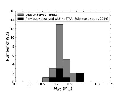
Figure 2: Stacked histogram of the mass distribution of WDs in mCVs. Legacy targets from this work are in grey, whilst masses derived from previous NuSTAR observations (Suleimanov et al., 2019) are in black.

The mass distribution of WDs in the 26 mCVs observed by NuSTAR is presented in Fig. 2. The distribution peaks in the range 0.7–0.8 $M_{\odot}$. We also present the mCV mass distribution alongside WD mass distributions for different populations of WDs in Fig. 3 in order to draw some comparisons. In the upper panel, we plot the mass distribution of WDs in non-magnetic CVs. To do this we use a sample of CVs that are considered to have ‘robust’ mass measurements (Zorotovic et al., 2011, their table 1) and remove the four mCVs from that sample, such that only non-magnetic systems remain, for a total of 27 sources. The non-magnetic WDs peak in the range 0.7–0.8 $M_{\odot}$ and have a weighted average $\bar{M}_{\rm WD}=0.80\pm 0.04$ $M_{\odot}$, with $\sigma=0.10$ $M_{\odot}$, consistent with the magnetic WD distribution.

In the middle panel of Fig. 3 we show the mass distribution of isolated WDs. This distribution consists of spectroscopically confirmed WDs from Data Release 12 of the Sloan Digital Sky Survey (SDSS-DR12; see Kepler et al., 2016b, a). We choose hydrogen atmosphere (DA) WDs with a spectral signal-to-noise ratio (S/N) $\geq 15$ for a total of 492 WDs with a weighted average $\bar{M}_{\rm WD}=0.53\pm 0.03$ $M_{\odot}$and $\sigma=0.15$ $M_{\odot}$. The isolated WD distribution peaks in the range 0.5–0.7 $M_{\odot}$ and, from Fig. 3, it is clear just by eye that isolated WDs are preferentially lower mass than both magnetic and non-magnetic WDs in CVs.

The final distribution we compare to, in the lower panel of Fig. 3, is that of detached post-common-envelope binaries (PCEBs) - the stage in binary evolution that immediately precedes CV formation (Paczynski, 1976). We plot this distribution from the sample presented by Zorotovic et al. (2011) in their table 2. We highlight in particular a subset of the sample that have CV formation times shorter than the age of the Galaxy and will undergo stable mass-transfer and thus are representative of the present-day CV population, the so-called ‘pre-CVs’ (Zorotovic et al., 2011). The PCEB distribution peaks in the range 0.5–0.6 $M_{\odot}$ and the pre-CVs in the range 0.6–0.7 $M_{\odot}$, similar to the isolated WDs, though with a longer tail. The PCEBs and Pre-CVs have a weighted average $\bar{M}_{\rm WD}=0.50\pm 0.02$ ($\sigma=0.11$) and $0.53\pm 0.04$ ($\sigma=0.12$) $M_{\odot}$, respectively.

To compare the mCV distribution with other WD distributions we utilise the $k$-sample Anderson-Darling test, where $k=2$ in this instance. We adopt the null hypothesis that two samples are drawn from the same distribution. In comparing the mCVs and non-magnetic CVs (Zorotovic et al., 2011), we find that we cannot reject the null hypothesis, down to the 10% level. When comparing the mCV mass distribution with that of the Kepler et al. (2016b) isolated WDs, we find that they must be drawn from two separate distributions, rejecting the null hypothesis at the $<0.1$% level. Finally, we find that when we compare the mCV and Zorotovic et al. (2011) PCEB and Pre-CV samples, we can reject the null hypothesis at the $<0.1$% level in both instances. Statistically, it appears that mCVs and non-magnetic CVs exhibit consistent mass distributions, both distinct from those of other types of WD, confirming, and expanding upon, the findings of Zorotovic et al. (2011).

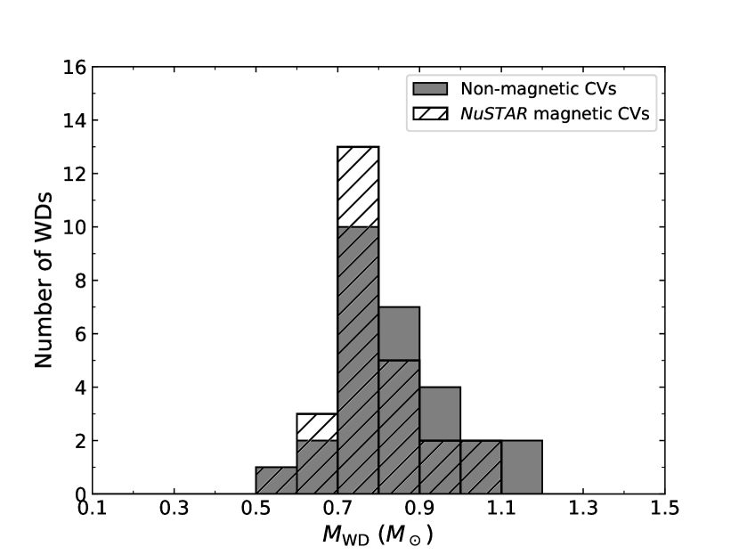
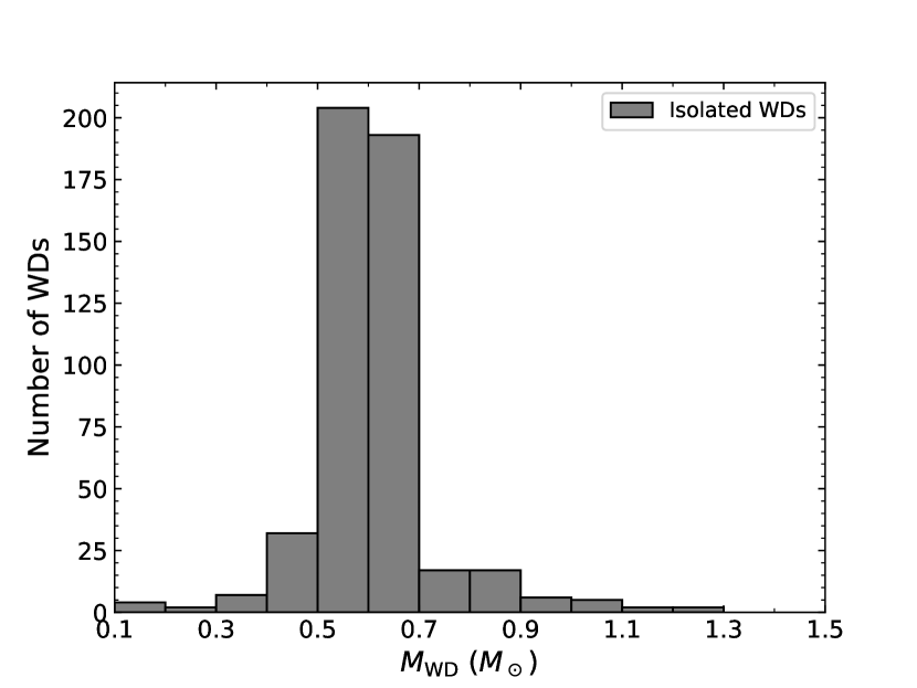
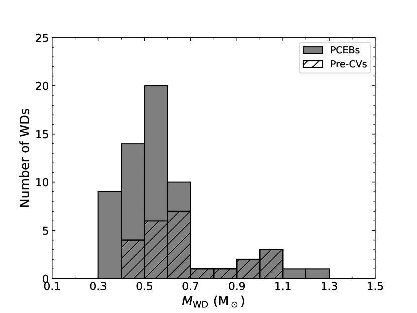
Figure 3: Upper Panel: Histograms of WD masses from mCVs (this work plus Suleimanov et al., 2019, hatched) and the non-magnetic CVs (grey; Zorotovic et al., 2011). Middle Panel: Histogram of masses of isolated WDs from the Sloan Digital Sky Survey (Kepler et al., 2016b). Lower Panel: Histogram of WD masses from post-common-envelope binaries (grey) and a subset of that sample considered to be representative of progenitors of current CVs (‘pre-CVs;’ Zorotovic et al., 2011, hatched).

3.2 Comparisons with Swift/BAT-measured masses

Suleimanov et al. (2019) analyse a sample of 35 IPs detected in the 70 month Swift/BAT survey. They use NuSTAR to measure the masses for 10 of them (three Legacy targets and 7 previously observed with NuSTAR). Of the remaining 25 IPs in that sample, 13 now have NuSTAR-derived masses. We directly compare the masses we derive from NuSTAR spectra with those from Swift/BAT spectra in Fig. 4.

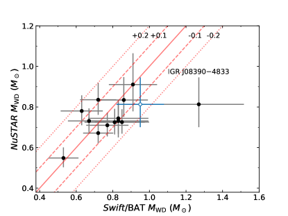
Figure 4: Comparison of WD masses derived by applying the PSR model to NuSTAR spectra, with those obtained by applying the same model to Swift/BAT spectra (Suleimanov et al., 2019). The solid line is the function $M_{\rm WD}$ (NuSTAR) = $M_{\rm WD}$ (BAT), the dashed lines show $M_{\rm WD}$ (NuSTAR) = $M_{\rm WD}$ (BAT) $\pm 0.1$ $M_{\odot}$ and the dotted lines show $M_{\rm WD}$ (NuSTAR) = $M_{\rm WD}$ (BAT) $\pm 0.2$ $M_{\odot}$. We also plot the value of $M_{\rm WD}$ of IGR J08390$-$4833 as measured by INTEGRAL (Bernardini et al., 2012) with a blue, open circle.

The majority of the derived masses are broadly consistent between NuSTAR and Swift/BAT, with a typical scatter $\sim\pm 0.1$ $M_{\odot}$. However, Fig. 4 shows one major outlier: IGR  J08390$-$4833. Suleimanov et al. (2019) measure $M_{\rm WD}$=$1.27\pm 0.25$ $M_{\odot}$ (uncertainty recalculated to 90% confidence), compared to the $0.81^{+0.13}_{-0.11}$ $M_{\odot}$ derived from the NuSTAR spectra. Previous measurements with INTEGRAL imply a mass consistent with the NuSTAR-derived one ($M_{\rm WD}$=$0.95\pm 0.13$ $M_{\odot}$; Bernardini et al., 2012).

IGR J08390$-$4833 is located in a complicated region of the sky, where contributions from the Vela supernova remnant (SNR; with which the IP is spatially coincident) and other nearby X-ray sources may cause higher than typical systematic uncertainties for poor angular-resolution measurements, such as those by Swift-BAT. Indeed, upon closer inspection of the modeled Swift/BAT spectrum of IGR J08390$-$4833, we find that the fit is poor, with a strong excess beyond $30$ keV that can likely be attributed to emission from the SNR and/or other nearby X-ray sources. We therefore suggest that the value in Table 2 is more representative of the true mass of the WD in IGR J08390$-$4833, as we were able to isolate and extract photons from the source and background by studying the NuSTAR image.

3.3 Comparisons with masses derived from the iron line complex

Fujimoto & Ishida (1997) and Ezuka & Ishida (1999) showed that the Fe complex in the $\sim$6–7 keV region of mCV spectra can be used to constrain $M_{\rm WD}$. This is achieved by measuring the intensity ratio of the H-like (7.0 keV) and He-like (6.7 keV) components of the Fe complex, which is correlated with the temperature of the PSR. Using the NuSTAR observations of mCVs available at the time (some of which are Legacy targets), Xu et al. (2019) applied a similar methodology to derive $M_{\rm WD}$ for a number of systems. We directly compare the masses derived using the PSR model (Suleimanov et al., 2019, and this work) with those derived using the Fe line ratio method on the same NuSTAR data (combined with Suzaku data, Xu et al., 2019) in Fig. 5.

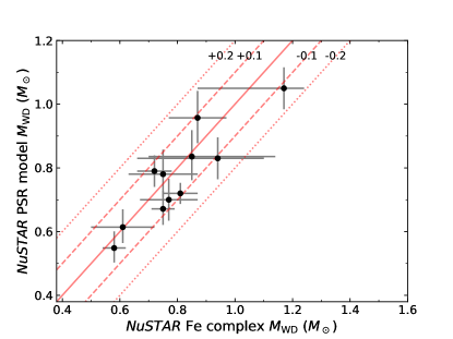
Figure 5: Comparison of WD masses derived from applying the PSR model to the 20–78 keV NuSTAR spectra ($y$-axis) with those derived by measuring the intensity ratio of the 7.0 and 6.7 keV Fe lines (Xu et al., 2019, $x$-axis), using the same NuSTAR data combined with archival Suzaku data. The solid line is the function $M_{\rm WD}$ (PSR) = $M_{\rm WD}$ (Fe), the dashed lines show $M_{\rm WD}$ (PSR) = $M_{\rm WD}$ (Fe) $\pm 0.1$ $M_{\odot}$ and the dotted lines show $M_{\rm WD}$ (PSR) = $M_{\rm WD}$ (Fe) $\pm 0.2$ $M_{\odot}$.

The PSR model produces results consistent (within 90% uncertainties) with those of Xu et al. (2019), though we note that the PSR model results in smaller uncertainties. The completion of the Legacy survey, which was still in progress at the time of publication of Xu et al. (2019), adds 13 more mCVs to the NuSTAR archive. In future studies of the Legacy data we will be able to examine if this consistency between the two methodologies holds for all mCVs.

3.4 Caveats of the Modeling

3.4.1 Choice of Background Extraction Region

At high energies, the X-ray background becomes more dominant relative to the source photons. In mCVs, where the high energy turnover of the spectrum informs the derived $M_{\rm WD}$, it is therefore crucial that the background is measured correctly. We experimented by extracting background spectra for different regions (both on different detector chips and on the same chip as the source) for a subset of targets in the Legacy sample and applying the PSR model. We find that the derived mass remains consistent within uncertainties with the values detailed in Table 2.

3.4.2 Magnetic Field Strength

The Suleimanov et al. (2019) PSR model assumes that the dominant cooling mechanism in the PSR is thermal emission (i.e. Brehmsstrahlung). However, if the WD is highly magnetized ($B\gtrsim 20$ MG, but note the dependence on $M_{\rm WD}$ and specific accretion rate; see fig. 4 of Wu et al., 1994) then we might expect cyclotron cooling to compete with thermal emission. In this case, the PSR will be fainter in hard X-rays compared to the model prediction and the resultant mass will be underestimated.

Magnetic field strength measurements for IPs are rare. However, some of our targets do have optical polarisation measurements that have led to estimates of $B$. Of the IPs in the full NuSTAR sample, V405 Aur, V2400 Oph, RX J2133.7$+$5107 and PQ Gem have been suggested to contain WDs with $B\gtrsim 20$ MG (see Ferrario et al., 2015, and references therein). The two APs in our target list, V1432 Aql and BY Cam, are very close to being polars and are thus expected to be highly magnetic ($B\gtrsim 30$ MG; Ferrario et al., 2015, and references therein). Therefore, the masses of these WDs may be slightly underestimated. Though it is difficult to quantify the mass difference, due to the uncertainty in measurements of $B$ from optical polarimetry, taking cyclotron cooling into account would only push the mass distribution higher. Thus, the conclusion that the mCV mass distribution is distinct from that of PCEBs and isolated WDs remains valid.

3.4.3 Shock height

In our analysis, we have assumed that the shock is sufficiently close to the white dwarf surface such that the difference of the gravitational potential between the surface and the shock can be ignored. In reality, the shock can never be exactly at the surface. Here we investigate the systematic errors this may introduce to our white dwarf mass estimates.

As spectroscopy is relatively unaffected by shock heights $h_{\rm sh}\sim 0.1$ $R_{\rm WD}$, we instead investigate the shock height in our sample of IPs using their hard X-ray (10–30 keV) spin modulation. At these energies, absorption, the predominant cause of spin modulation below 10 keV, has limited effects. Geometric effects due to tall shocks, on the other hand, can result in a strong hard X-ray spin modulation regardless of photon energy (Mukai, 1999). This effect has been invoked to explain the spin modulation in IPs V709 Cas (de Martino et al., 2001) and EX Hya (Luna et al., 2018).

The characteristics of spin modulation due to tall shocks are a large amplitude, and modulations that often exhibit flat tops or flat bottoms (see e.g. V709 Cas; de Martino et al., 2001). Tall shocks lead to spin modulation because there is a range of viewing angles at which you see the emission from both shocks, so the maximum observed intensity can be twice the minimum. Lower spin modulation amplitude is possible when the footprint of the emission region is large enough that each pole is seen at a range of viewing angles, some allowing visibility of only one pole, others for both poles to be observable simultaneously. Small amplitude modulations require that poles largely remain in the one-pole only viewing zone with at most small, partial excursions into the two-pole viewing zone, or vice versa. This is likely to result in flat-bottomed (flat-topped) light curves.

We have examined the spin-folded 10–30 keV light curves of our targets. The APs V1432 Aql and BY Cam have large-amplitude modulations, as expected, since they are presumed to accrete onto one pole at a time (Staubert et al., 2003; Pavlenko et al., 2013). The IPs in our sample have low-amplitude modulations and do not collectively fit our expectations for tall shock systems. They all appear to show small but statistically significant spin modulations, of order $\pm$10% of the mean. The spin modulations are sometimes single peaked, sometimes double-peaked, and sometimes complex. Since spectral fits below 10 keV often indicate the presence of absorber components with hydrogen column density $N_{\rm H}$ up to several times 10²³ cm^-2, or Compton optical depths of a few tenths of unity, we believe that the observed level of hard X-ray absorption can be expected due to variable complex absorption.

Diametrically opposite X-ray emission regions 0.1 $R_{\rm WD}$ above the surface are observable for viewing angles 65–115^∘. We argue that this is not generally the case for IPs in our sample, as it would frequently lead to obvious symptoms of a tall shock, as has been observed in V709 Cas (Mukai et al., 2015). The range is 82–98^∘ for emission regions 0.01 $R_{\rm WD}$ above the surface. This range of viewing angle is sufficently small compared to the expected angular extent of the emission region that it is plausible for the resulting hard X-ray modulation to be smooth (i.e., not flat-topped or flat-bottomed) and small in amplitude, as we argue. This line of reasoning suggests that the systematic uncertainties due to tall shocks for our sample, as a group, is of order a few percent.

We can extrapolate the case of EX Hya to place rough estimates on the shock heights of some of the mCVs in our sample and test the above discussion. Luna et al. (2018) estimate a shock height $h_{\rm sh}\gtrsim 0.9$ $R_{\rm WD}$ for EX Hya, which exhibits a luminosity $L\sim 8\times 10^{31}$ erg s^-1 (Suleimanov et al., 2019). Shock height $h_{\rm sh}$ is inversely proportional to local mass accretion rate (Mukai, 1999). If we assume that the footprint area of the shock above the surface of the WD is the same for all mCVs, then $h_{\rm sh}$ varies inversely with overall mass accretion rate ($\dot{M}$) and therefore luminosity (along with a mass dependence). Based on this luminosity dependence, the faintest mCV in our target list, BY Cam with a luminosity $L=1.3\times 10^{33}$ erg s^-1, can be estimated to have $h_{\rm sh}\sim 0.06$ $R_{\rm WD}$, and brighter mCVs should have shorter shocks. The assumption that the footprint area is constant between sources is not completely secure, it is unclear how they vary amongst mCVs with different values of $B$ and $P_{\rm spin}$ (for example see e.g. Scaringi et al., 2010). Nevertheless, we may use the above extrapolation as an order of magnitude estimate of $h_{\rm sh}$, showing that systematic uncertainties in mass due to tall shocks should typically be of order a few percent.

This does not preclude the possibility of a more significant systematic error for individual objects. Among the Legacy sample, the hard X-ray spin modulation amplitude is of order $\pm$20% or greater for IGR J16547$-$1916, AO Psc, V405 Aur and FO Aqr. These are the IPs for which larger systematic errors are most likely.

The conclusion that WDs in IPs are more massive than in the field remains secure in any case, since tall shock effects can only lead to underestimates of $M_{\rm WD}$.

3.5 Selection Effects

With any survey of a specific class of astrophysical objects, one must consider the possible biases that may arise from the way the sample is selected. We discuss potential selection effects of our sample below and any subsequent effects they may have on our results.

3.5.1 Source flux

When devising the NuSTAR Legacy Survey of mCVs, we chose our sample based on the flux in the Swift/BAT 70 month catalogue (Baumgartner et al., 2013; Mukai, 2017). We chose the 25 brightest mCVs (in the BAT energy band; 14–195 keV) that had not previously been observed by NuSTAR, such that the limiting flux of our sample is $\sim 1.7\times 10^{-11}$ erg cm^-2 s^-1. Of the 25 initial targets, two were not observed (IGR J16500-3307 and IGR J04571+4527), two were not detected by NuSTAR (DO Dra and IGR J14536-5522) and two did not provide high enough S/N spectra to accurately constrain the mass using the method described in Section 2 (XY Ari and RX J2015.6+3711).

It could be assumed that, considering the sample is flux selected in the hard-X-ray band, the results may be biased towards higher masses. Though it is impossible to remove all potential bias arising from a flux-limited sample, our target selection seeks to reduce bias towards higher masses as much as possible. Suleimanov et al. (2019) measure masses for 35 objects from the Swift/BAT 70 month catalogue, which is the majority of the confirmed IPs in the catalogue. Their limiting flux is approximately half of ours (V1033 Cas; $8.43\times 10^{-12}$ erg cm^-2 s^-1; Mukai, 2017). Of those 35 IPs, there are now NuSTAR-measured masses for 23 of them, and we find that they generally agree with the Swift/BAT-measured masses but with smaller uncertainties (Fig. 4; also fig. 8 of Suleimanov et al., 2019). We can therefore reasonably assume that the remaining sources below our flux threshold have accurate Swift/BAT-measured masses, and these remaining sources are not biased toward any mass, high or low. In addition, there are only five confirmed IPs that are not detected by Swift/BAT (HT Cam, DW Cnc, UU Col, V1323 Her and WX Pyx). The limited X-ray information available regarding these objects suggests that they exhibit a range of shock temperatures (e.g. Schlegel, 2005; de Martino et al., 2006; Nucita et al., 2019) and therefore likely a range of masses. Any mass bias that exists due to the way in which we selected our sample is unlikely to be large.

However, we must make it clear that our sample selection does not preclude the existence of a population of (possibly low-mass) mCVs that may not have been identified as such due to their non-detection by X-ray observatories. This cannot be mitigated with statistical analysis and we base our results and conclusions on the known, visible population of mCVs.

3.5.2 Origin of the target’s X-ray discovery

Many of the X-ray observatories that discovered the mCVs in this work operate at hard X-ray energies. For example, all of the ‘IGR’ labelled IPs in our sample were discovered by the IBIS instrument onboard INTEGRAL, which operates at energies $>15$ keV. Considering the fraction of the total flux emitted in the hard band increases with $M_{\rm WD}$, hard X-ray instruments are more likely to detect massive WDs. Though a number of sources in the full NuSTAR sample were first detected in X-rays by ROSAT (0.1–2 keV; Truemper, 1982), the majority were discovered by instruments with some hard X-ray sensitivity (e.g. Ariel V; 1.5–20 keV, Uhuru; 2–20 keV and HEAO-1; 0.25–25 keV). We cannot discount the possibility of a bias towards higher masses. Though we note here that the five IGR sources in the full NuSTAR sample in addition to V667 Pup which was discovered by Swift/BAT ($>15$ keV), range from $M_{\rm WD}$=0.69–1.06 $M_{\odot}$, similar to the 8 ROSAT-discovered sources (0.61–1.05 $M_{\odot}$).

3.6 The CV mass problem

Considering the discussion above, we have shown that mCVs, like their non-magnetic counterparts, are preferentially more massive than both isolated WDs and PCEBs, consistent with previous surveys with non-imaging hard X-ray telescopes (e.g. Yuasa et al., 2010; Bernardini et al., 2012; Suleimanov et al., 2019). Whilst we cannot dismiss the possibility that unidentified systematic uncertainties in the mass measurements of both non-magnetic and magnetic systems contribute to this observed difference, we can only discuss the origin of the discrepancy in the context of the existing observations. Therefore, how do we reconcile this with theoretical predictions? The classic picture of CV formation starts with a wide main-sequence – main-sequence (MS – MS) binary, whereby one of the binary components becomes a red giant and fills its Roche lobe, initiating mass transfer on to the companion. The unstable nature of this mass transfer leads to a common envelope (CE) phase and the orbital separation is reduced through drag forces within the envelope. Once the envelope is expelled, what is left behind is a close (yet detached) WD – MS binary, i.e., the PCEB scenario discussed above. Upon further reduction of the binary separation (through angular momentum loss by a combination of gravitational radiation and magnetic braking; Knigge et al., 2011), the binary will then initiate the second mass transfer stage that defines CVs (Paczynski, 1976). A consequence of this evolutionary path is that WDs in CVs should have a (slightly) lower mean mass than that of isolated WDs (Politano, 1996).

We now know that observationally, this is not true. Zorotovic et al. (2011) show that $\bar{M}_{\rm WD}=0.83$ $M_{\odot}$ from a non-magnetic CV sample free of observational biases related to WD mass. We show from spectral modeling of high quality NuSTAR observations that the weighted average mass of WDs in mCVs is similarly high, $\bar{M}_{\rm WD}=0.77\pm 0.02$ $M_{\odot}$, with $\sigma=0.10$ $M_{\odot}$. Matters are complicated further by the fact that studies of PCEBs, i.e. the precursor to CVs, have revealed that the observed WD mass distribution of these objects is in good agreement with theoretical predictions (e.g. Zorotovic et al., 2011; Toonen & Nelemans, 2013; Camacho et al., 2014), meaning that the problem is not due to an underlying misunderstanding of CE evolution.

Mass-growth does not appear to solve the problem, nor does a short phase of thermal timescale mass transfer, at least for non-magnetic CVs (Wijnen et al., 2015). It has long been suggested that nova explosions should prevent mass-growth from occurring, if the amount of mass expelled in the explosion is more than the amount accreted between outbursts, as is predicted by a number of theoretical models (Prialnik & Kovetz 1995; Yaron et al. 2005; but see below). Schreiber et al. (2016) suggest that consequential angular momentum loss (CAML) may solve the WD mass problem in non-magnetic CVs. The CAML hypothesis suggests that angular momentum loss driven by mass transfer (e.g. frictional angular momentum loss through nova explosions) is more effective in lower mass systems, resulting in mass transfer becoming unstable in such systems. CVs therefore have preferentially higher mass WDs. Our results may indicate that CAML works similarly for both magnetic and non-magnetic CVs.

Another potential solution to the CV mass problem could be that the amount of mass expelled by a nova explosion is less than some theoretical models predict. According to a number of simulations (e.g. Hillman et al., 2015), there is a region of the parameter space where $M_{\rm WD}$ grows after successive accretion–nova cycles. While this region was limited to very high mass WDs in most models, hence did not address the observational discrepancy, more recent hydrodynamical simulations of classical novae by Starrfield et al. (2020) suggest that WDs with masses in the range 0.6–1.35 $M_{\odot}$ can grow in mass through accretion–nova cycles. The fact that nova models are seen to contradict one another on the topic of mass-growth, shows that there is no clear consensus on the matter.

4 Conclusions

We have conducted the first dedicated survey of mCVs with an imaging hard X-ray telescope in order to derive the mass distribution of magnetic WDs. Adding the results of this survey to those of the 7 IPs previously observed by NuSTAR (Suleimanov et al., 2019) brings the total number of accreting magnetic WD masses constrained with NuSTAR to 26. This is the largest single sample of mCV masses constrained with imaging telescopes to date.

We utilized the PSR X-ray spectral model (Suleimanov et al., 2016, 2019) to derive $M_{\rm WD}$. For FO Aqr, we confirmed the Suleimanov et al. (2019) estimate of $R_{\rm m}$ based on the measurement of a break in the aperiodic power spectrum. We find the weighted average of all 26 mCVs to be $\bar{M}_{\rm WD}=0.77\pm 0.02$ $M_{\odot}$ with a standard deviation of 0.10 $M_{\odot}$. Statistically, the mass distribution is consistent with that of WDs in non-magnetic CVs, i.e. accreting WDs, whether magnetic or not, appear to preferentially have higher masses than both isolated WDs and the precursors to CVs, PCEBs. This compounds the CV mass problem, i.e. the discrepancy between observations and theory surrounding masses of accreting WDs. We speculate that consequential angular momentum loss (Schreiber et al., 2016) may play a role in this discrepancy, but also note that our understanding of how $M_{\rm WD}$ changes over accretion–nova cycles may also be incomplete.

4.1 Future Work

The Legacy dataset that resulted in this work is extensive, and PSR modeling of the $>20$ keV spectra is just one of the analysis approaches we can take. Xu et al. (2019) showed, with a small number of NuSTAR spectra, that there is a wealth of information embedded within the Fe line complex that can lead to an independent derivation of PSR temperature and therefore mass. In addition a study of the full 3–78 keV spectra, will allow us to conduct an in-depth analysis of reflection and partial covering in mCVs, allowing estimates of the shock height, as well as an alternative spectral fitting method to measure $M_{\rm WD}$.

Data Availability Statement

The data underlying this article are publicly available in the NuSTAR Master Catalog (NUMASTER) at https://heasarc.gsfc.nasa.gov/W3Browse/nustar/numaster.html. The Observation ID for each target is listed in Table 1.

Appendix A Spectral figures

We plot the NuSTAR spectra of the Legacy survey targets (excluding FO Aqr; see Fig. 1 in Fig. 6.

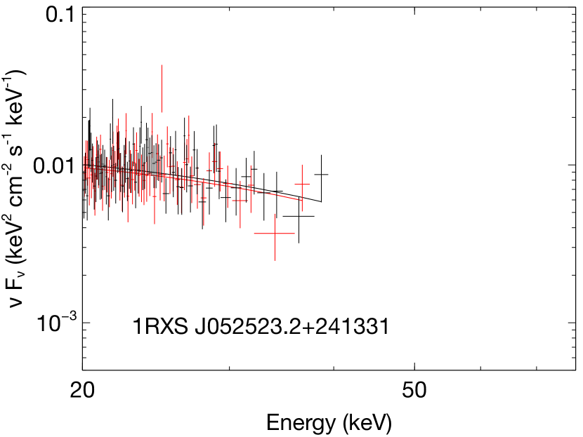
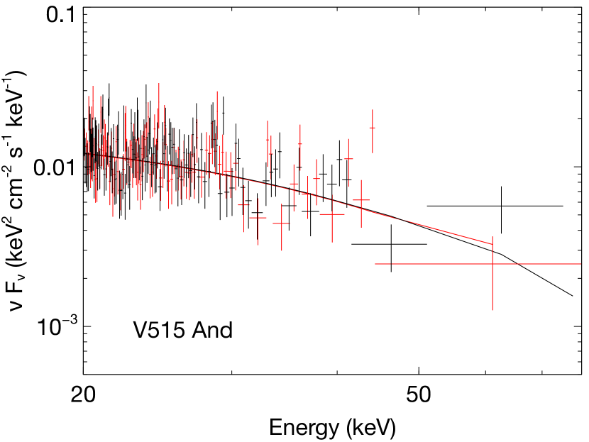
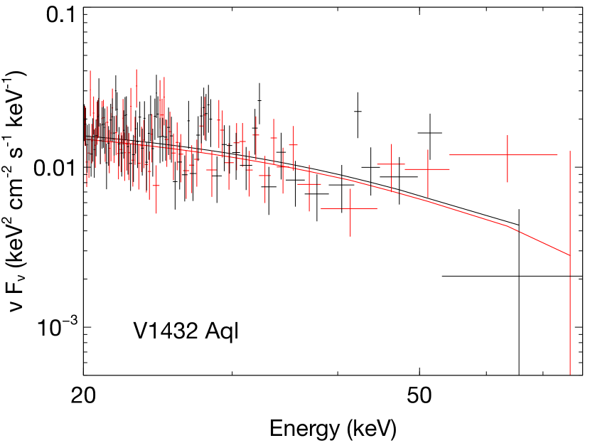
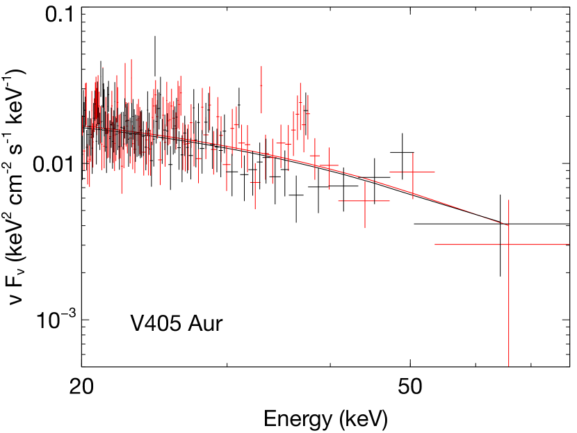
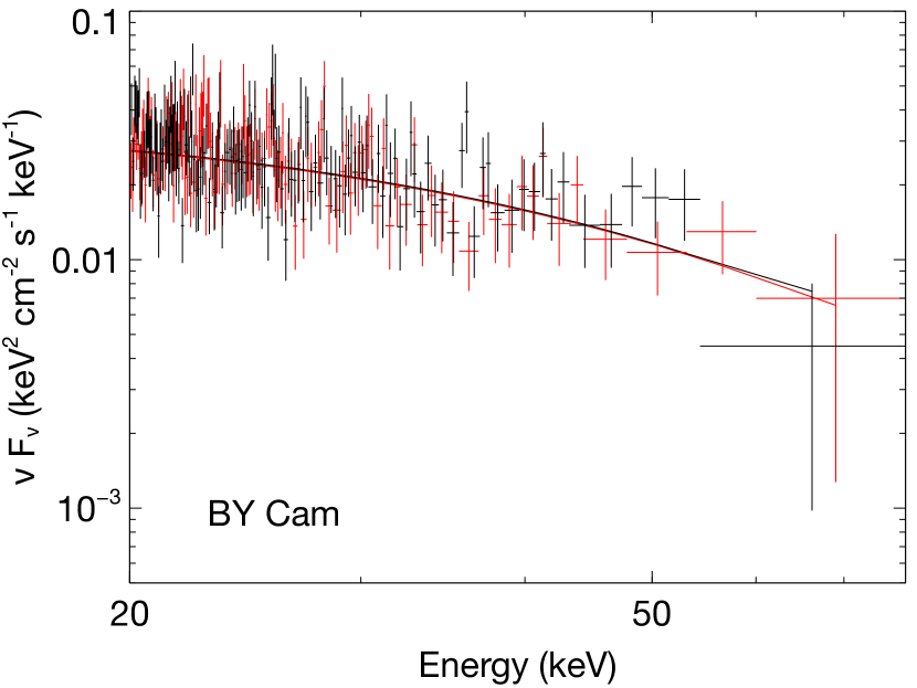
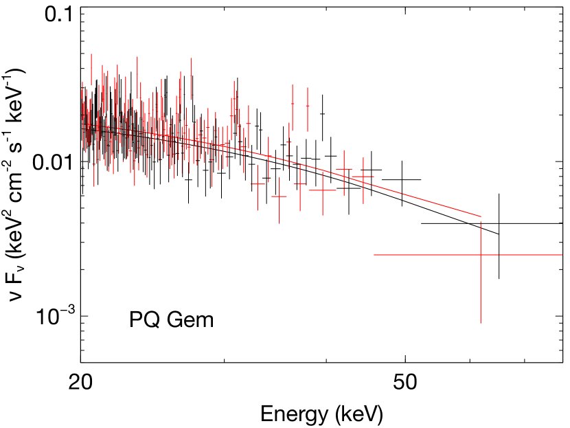
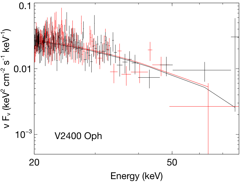
Figure 6: NuSTAR FPMA (black) and FPMB (red) spectra of the Legacy survey targets (excluding FO Aqr; see Fig. 1), fit with the Suleimanov et al. (2019) PSR model and plotted unfolded in $\nu$F_ν space. Because the IP V1062 Tau was split into two separate observations, we fit two spectra from each FPM simultaneously. In this case we also plot FPMA (green) and FPMB (blue) of the second observation.

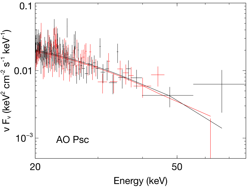
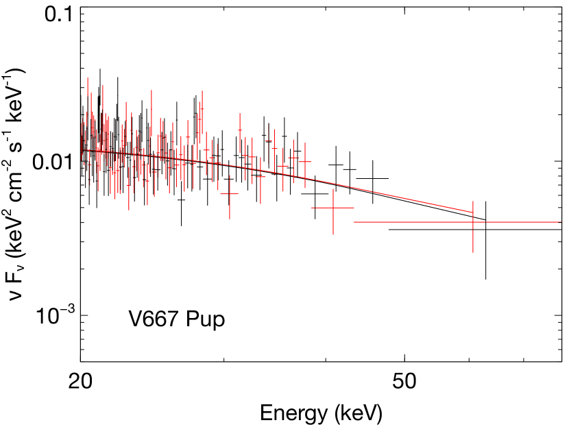
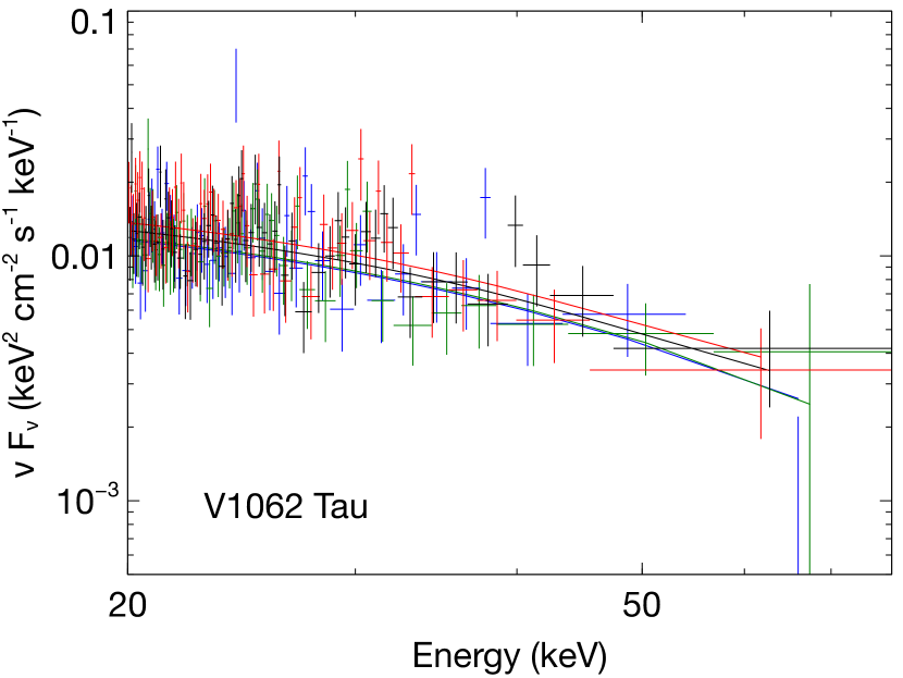
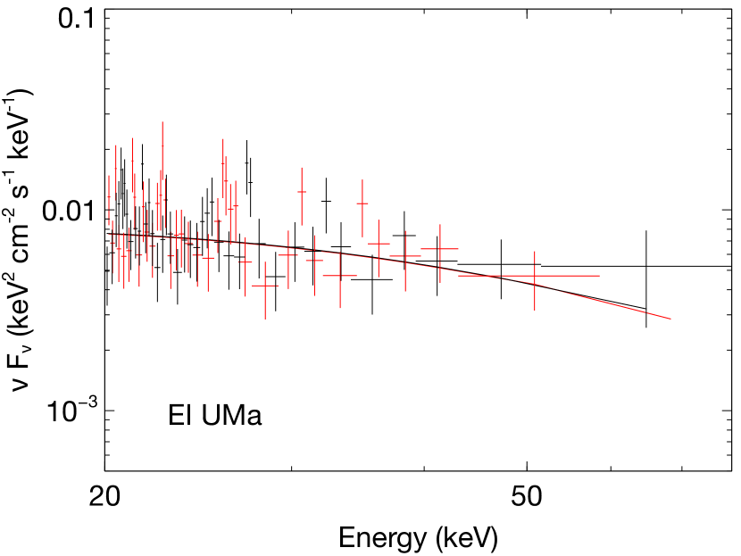
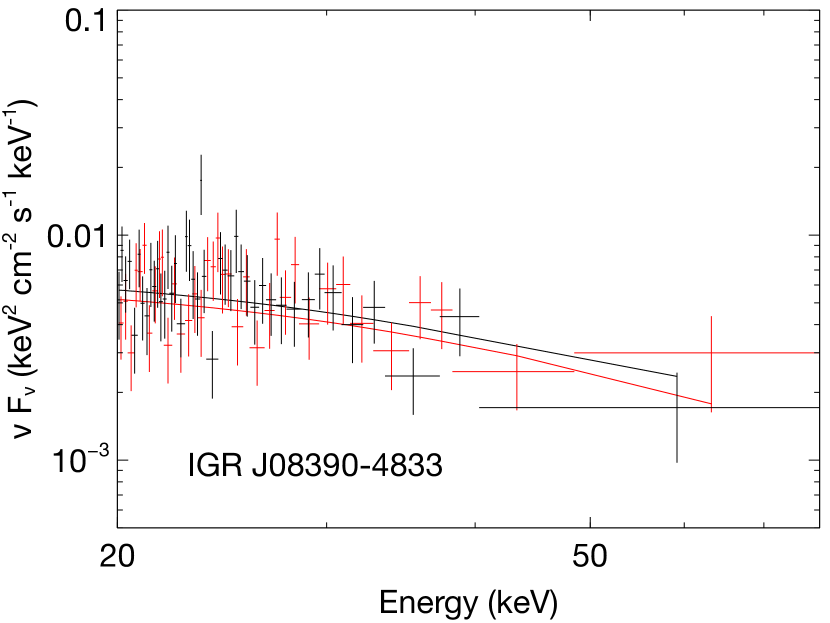
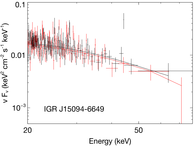
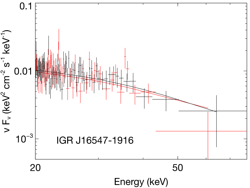
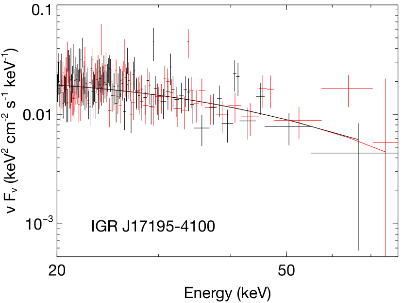
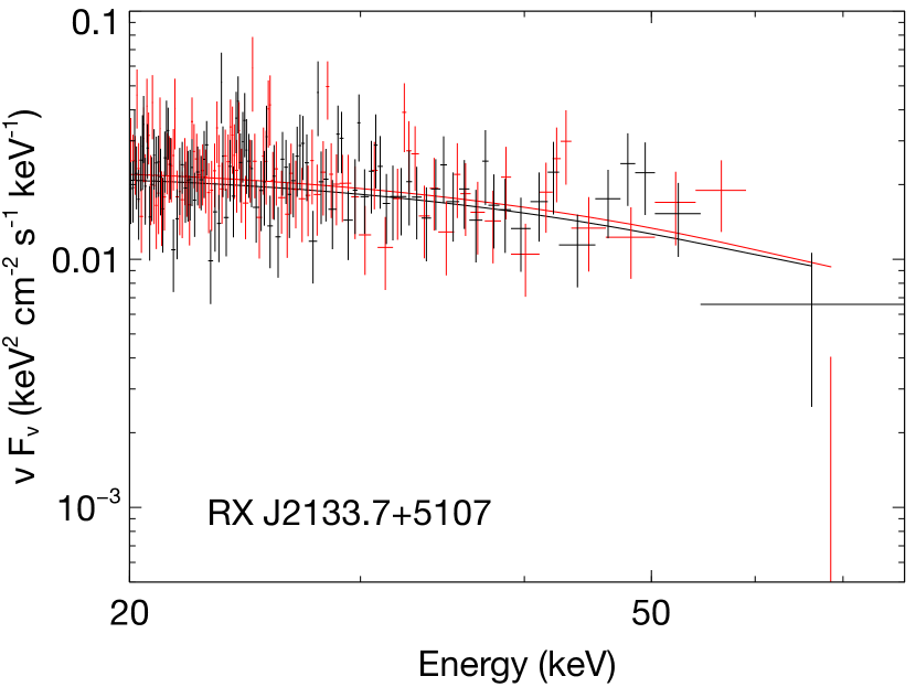
Figure 7: (cont.)

References

- Aizu (1973) Aizu K., 1973, Progress of Theoretical Physics, 49, 1184
- Arnaud (1996) Arnaud K. A., 1996, in Jacoby G. H., Barnes J., eds, Astronomical Society of the Pacific Conference Series Vol. 101, Astronomical Data Analysis Software and Systems V. p. 17
- Bailer-Jones et al. (2018) Bailer-Jones C. A. L., Rybizki J., Fouesneau M., Mantelet G., Andrae R., 2018, AJ, 156, 58
- Barthelmy et al. (2005) Barthelmy S. D., et al., 2005, Space Sci. Rev., 120, 143
- Baumgartner et al. (2013) Baumgartner W. H., Tueller J., Markwardt C. B., Skinner G. K., Barthelmy S., Mushotzky R. F., Evans P. A., Gehrels N., 2013, ApJS, 207, 19
- Belloni & Schreiber (2020) Belloni D., Schreiber M. R., 2020, MNRAS, 492, 1523
- Bernardini et al. (2012) Bernardini F., de Martino D., Falanga M., Mukai K., Matt G., Bonnet-Bidaud J. M., Masetti N., Mouchet M., 2012, A&A, 542, A22
- Bradt et al. (1993) Bradt H. V., Rothschild R. E., Swank J. H., 1993, A&AS, 97, 355
- Brunschweiger et al. (2009) Brunschweiger J., Greiner J., Ajello M., Osborne J., 2009, A&A, 496, 121
- Camacho et al. (2014) Camacho J., Torres S., García-Berro E., Zorotovic M., Schreiber M. R., Rebassa-Mansergas A., Nebot Gómez-Morán A., Gänsicke B. T., 2014, A&A, 566, A86
- Coti Zelati et al. (2016) Coti Zelati F., Rea N., Campana S., de Martino D., Papitto A., Safi-Harb S., Torres D. F., 2016, MNRAS, 456, 1913
- Cropper (1990) Cropper M., 1990, Space Sci. Rev., 54, 195
- Cropper et al. (1998) Cropper M., Ramsay G., Wu K., 1998, MNRAS, 293, 222
- Cropper et al. (1999) Cropper M., Wu K., Ramsay G., Kocabiyik A., 1999, MNRAS, 306, 684
- Done & Magdziarz (1998) Done C., Magdziarz P., 1998, MNRAS, 298, 737
- Ezuka & Ishida (1999) Ezuka H., Ishida M., 1999, ApJS, 120, 277
- Ferrario et al. (2015) Ferrario L., de Martino D., Gänsicke B. T., 2015, Space Sci. Rev., 191, 111
- Ferrario et al. (2020) Ferrario L., Wickramasinghe D. T., Kawka A., 2020, arXiv e-prints, p. arXiv:2001.10147
- Fujimoto & Ishida (1997) Fujimoto R., Ishida M., 1997, ApJ, 474, 774
- Fukazawa et al. (2009) Fukazawa Y., et al., 2009, PASJ, 61, S17
- Gehrels et al. (2004) Gehrels N., et al., 2004, ApJ, 611, 1005
- Hailey et al. (2016) Hailey C. J., et al., 2016, ApJ, 826, 160
- Halpern et al. (2017) Halpern J. P., Bogdanov S., Thorstensen J. R., 2017, ApJ, 838, 124
- Harrison et al. (2013) Harrison F. A., et al., 2013, ApJ, 770, 103
- Hayashi & Ishida (2014) Hayashi T., Ishida M., 2014, MNRAS, 441, 3718
- Hellier (2014) Hellier C., 2014, in European Physical Journal Web of Conferences. p. 07001 (arXiv:1312.4779), doi:10.1051/epjconf/20136407001
- Hillman et al. (2015) Hillman Y., Prialnik D., Kovetz A., Shara M. M., 2015, MNRAS, 446, 1924
- Hillman et al. (2020) Hillman Y., Shara M. M., Prialnik D., Kovetz A., 2020, Nature Astronomy,
- Huppenkothen et al. (2016) Huppenkothen D., Bachetti M., Stevens A. L., Migliari S., Balm P., 2016, Stingray: Spectral-timing software (ascl:1608.001)
- Huppenkothen et al. (2019) Huppenkothen D., et al., 2019, ApJ, 881, 39
- Katz (1977) Katz J. I., 1977, ApJ, 215, 265
- Kennedy et al. (2017) Kennedy M. R., Garnavich P. M., Littlefield C., Callanan P., Mukai K., Aadland E., Kotze M. M., Kotze E. J., 2017, MNRAS, 469, 956
- Kepler et al. (2016a) Kepler S. O., et al., 2016a, VizieR Online Data Catalog, p. J/MNRAS/455/3413
- Kepler et al. (2016b) Kepler S. O., et al., 2016b, MNRAS, 455, 3413
- Kilic et al. (2018) Kilic M., Hambly N. C., Bergeron P., Genest-Beaulieu C., Rowell N., 2018, MNRAS, 479, L113
- Knigge et al. (2011) Knigge C., Baraffe I., Patterson J., 2011, ApJS, 194, 28
- Littlefield et al. (2015) Littlefield C., et al., 2015, MNRAS, 449, 3107
- Luna et al. (2018) Luna G. J. M., Mukai K., Orio M., Zemko P., 2018, ApJ, 852, L8
- Madsen et al. (2017) Madsen K. K., Christensen F. E., Craig W. W., Forster K. W., Grefenstette B. W., Harrison F. A., Miyasaka H., Rana V., 2017, Journal of Astronomical Telescopes, Instruments, and Systems, 3, 1
- Matsuoka et al. (2009) Matsuoka M., et al., 2009, PASJ, 61, 999
- Matthews et al. (2007) Matthews O. M., Speith R., Wynn G. A., West R. G., 2007, MNRAS, 375, 105
- Mitsuda et al. (2007) Mitsuda K., et al., 2007, PASJ, 59, 1
- Mukai (1999) Mukai K., 1999, in Hellier C., Mukai K., eds, Astronomical Society of the Pacific Conference Series Vol. 157, Annapolis Workshop on Magnetic Cataclysmic Variables. p. 33
- Mukai (2017) Mukai K., 2017, PASP, 129, 062001
- Mukai et al. (2015) Mukai K., Rana V., Bernardini F., de Martino D., 2015, ApJ, 807, L30
- Nauenberg (1972) Nauenberg M., 1972, ApJ, 175, 417
- Nucita et al. (2019) Nucita A. A., Conversi L., Licchelli D., 2019, MNRAS, 484, 3119
- Paczynski (1976) Paczynski B., 1976, in Eggleton P., Mitton S., Whelan J., eds, IAU Symposium Vol. 73, Structure and Evolution of Close Binary Systems. p. 75
- Patterson (1994) Patterson J., 1994, PASP, 106, 209
- Patterson et al. (2020) Patterson J., et al., 2020, arXiv e-prints, p. arXiv:2001.07288
- Pavlenko et al. (2013) Pavlenko E., Andreev M., Babina Y., Malanushenko V., 2013, in Krzesiński J., Stachowski G., Moskalik P., Bajan K., eds, Astronomical Society of the Pacific Conference Series Vol. 469, 18th European White Dwarf Workshop.. p. 343
- Politano (1996) Politano M., 1996, ApJ, 465, 338
- Prialnik & Kovetz (1995) Prialnik D., Kovetz A., 1995, ApJ, 445, 789
- Ramsay et al. (2004) Ramsay G., Cropper M., Wu K., Mason K. O., Córdova F. A., Priedhorsky W., 2004, MNRAS, 350, 1373
- Rea et al. (2017) Rea N., et al., 2017, MNRAS, 471, 2902
- Revnivtsev et al. (2009) Revnivtsev M., Churazov E., Postnov K., Tsygankov S., 2009, A&A, 507, 1211
- Revnivtsev et al. (2011) Revnivtsev M., Potter S., Kniazev A., Burenin R., Buckley D. A. H., Churazov E., 2011, MNRAS, 411, 1317
- Rothschild et al. (1981) Rothschild R. E., et al., 1981, ApJ, 250, 723
- Scaringi et al. (2010) Scaringi S., et al., 2010, Monthly Notices of the Royal Astronomical Society, 401, 2207
- Schlegel (2005) Schlegel E. M., 2005, A&A, 433, 635
- Schmidt & Stockman (1991) Schmidt G. D., Stockman H. S., 1991, ApJ, 371, 749
- Schreiber et al. (2016) Schreiber M. R., Zorotovic M., Wijnen T. P. G., 2016, MNRAS, 455, L16
- Shaw et al. (2018) Shaw A. W., Heinke C. O., Mukai K., Sivakoff G. R., Tomsick J. A., Rana V., 2018, MNRAS, 476, 554
- Starrfield et al. (2020) Starrfield S., Bose M., Iliadis C., Hix W. R., Woodward C. E., Wagner R. M., 2020, ApJ, 895, 70
- Staubert et al. (2003) Staubert R., Friedrich S., Pottschmidt K., Benlloch S., Schuh S. L., Kroll P., Splittgerber E., Rothschild R., 2003, A&A, 407, 987
- Suleimanov et al. (2005) Suleimanov V., Revnivtsev M., Ritter H., 2005, A&A, 435, 191
- Suleimanov et al. (2016) Suleimanov V., Doroshenko V., Ducci L., Zhukov G. V., Werner K., 2016, A&A, 591, A35
- Suleimanov et al. (2019) Suleimanov V. F., Doroshenko V., Werner K., 2019, MNRAS, 482, 3622
- Toonen & Nelemans (2013) Toonen S., Nelemans G., 2013, A&A, 557, A87
- Truemper (1982) Truemper J., 1982, Advances in Space Research, 2, 241
- Warner (2003) Warner B., 2003, Cataclysmic Variable Stars. Cambridge Univ. Press, doi:10.1017/CBO9780511586491
- Wijnen et al. (2015) Wijnen T. P. G., Zorotovic M., Schreiber M. R., 2015, A&A, 577, A143
- Winkler et al. (2003) Winkler C., et al., 2003, A&A, 411, L1
- Wu et al. (1994) Wu K., Chanmugam G., Shaviv G., 1994, ApJ, 426, 664
- Xu et al. (2019) Xu X.-j., Yu Z.-l., Li X.-d., 2019, ApJ, 878, 53
- Yaron et al. (2005) Yaron O., Prialnik D., Shara M. M., Kovetz A., 2005, ApJ, 623, 398
- Yuasa et al. (2010) Yuasa T., Nakazawa K., Makishima K., Saitou K., Ishida M., Ebisawa K., Mori H., Yamada S., 2010, A&A, 520, A25
- Zorotovic et al. (2011) Zorotovic M., Schreiber M. R., Gänsicke B. T., 2011, A&A, 536, A42
- de Martino et al. (2001) de Martino D., et al., 2001, A&A, 377, 499
- de Martino et al. (2006) de Martino D., Matt G., Mukai K., Bonnet-Bidaud J. M., Burwitz V., Gänsicke B. T., Haberl F., Mouchet M., 2006, A&A, 454, 287
- de Martino et al. (2020) de Martino D., Bernardini F., Mukai K., Falanga M., Masetti N., 2020, Advances in Space Research, 66, 1209