Unifying framework for strong and fragile liquids via machine learning: a study of liquid silica

Abstract

The fragility of a glassforming liquid characterizes how rapidly its relaxation dynamics slow down with cooling. The viscosity of strong liquids follows an Arrhenius law with a temperature-independent barrier height to rearrangements responsible for relaxation, whereas fragile liquids experience a much faster increase in their dynamics, suggesting a barrier height that increases with decreasing temperature. Strong glassformers are typically network glasses, while fragile glassformers are typically molecular or hard-sphere-like. As a result of these differences at the microscopic level, strong and fragile glassformers are usually treated separately from a theoretical point of view. Silica is the archetypal strong glassformer at low temperatures, but also exhibits a mysterious strong-to-fragile crossover at higher temperatures. Here we show that softness, a structure-based machine learned parameter that has previously been applied to fragile glassformers provides a useful description of model liquid silica in the strong and fragile regimes, and through the strong-to-fragile crossover. Just as for fragile glassformers, the relationship between softness and dynamics is invariant and Arrhenius in all regimes, but the average softness changes with temperature. The strong-to-fragile crossover in silica is not due to a sudden, qualitative change in structure, but can be explained by a simple Arrhenius form with a continuously and linearly changing local structure. Our results unify the study of liquid silica under a single simple conceptual picture.

When cooled quickly enough, liquids can avoid crystallization and relax more and more slowly, eventually undergoing dynamical arrest on human time scales even as their structure remains similar to that of the liquid. In 1985, Angell suggested placing glassforming liquids into a spectrum from strong liquids to fragile liquids in the celebrated “Angell plot” Angell (1985, 1991); Salmon and Zeidler (2013). In strong liquids like silica, the dynamics of the liquid slow down as one would expect from an Arrhenius process. Most other liquids are fragile, however, and exhibit a much faster slowing of the dynamics. To complicate matters further, silica undergoes a strong-to-fragile crossover upon heating at around 3100-3300 K Saika-Voivod et al. (2001); Geske et al. (2016).

It has been shown that the non-Arrhenius behavior of a model fragile glassformer, a binary Lennard-Jones mixture known as the Kob-Andersen model Kob and Andersen (1994), can be captured by simple expression involving a structural quantity known as “softness”  Schoenholz et al. (2016). This quantity is obtained using machine learning to identify the linear combination of a set of structural quantities that correlates most strongly with rearrangements in the supercooled liquid. At any given moment, different particles have different softnesses described by a distribution. For three fragile glassformers, the Kob-Andersen model Schoenholz et al. (2017), the Weeks-Chandler-Andersen model Landes et al. (2019) and a model polymer glassformer Sussman et al. (2017), the relaxation time $\tau_{\alpha}$ can be expressed simply as Schoenholz et al. (2017)

$$\tau_{\alpha}\propto 1/P_{R}(\langle S\rangle),$$ (1)

where $P_{R}(S)$ is the probability density that a particle of softness $S$ will rearrange and $\langle S\rangle$ is the average softness of particles in the system. The rearrangement probability $P_{R}(S)$ is Arrhenius at each value of $S$, implying that particles of softness $S$ have a well-defined, temperature-independent free energy barrier to rearrangement $\Delta F(S)$. The barrier increases with decreasing $S$, so that particles with lower softness have a smaller propensity to rearrange. As the system cools, $\langle S\rangle$ decreases; this leads to slowing down of the relaxation time.

In this Letter, we show that the softness-based description of the dynamics outlined above for fragile glassformers also applies to a model of a strong glassformer, namely silica. Further, we show that this description can predict the dynamics not only of the low-temperature strong liquid, but also the strong-to-fragile crossover and the high temperature fragile liquid. Thus, our results suggest that the wide diversity of fragility observed in different liquids can be boiled down to the temperature dependence of a single machine-learned variable.

We model silica liquid using the potential of van Beest, Krame, and van Santen (BKS) Van Beest et al. (1990), which has been commonly used to study liquid Saika-Voivod et al. (2001); Horbach and Kob (1999) and amorphous silica Vollmayr and Kob (1996). A harmonic potential is used at small distances to prevent Si and O atoms from fusing together Vollmayr and Kob (1996). We confirm that this modification reliably prevents unphysical fusion events without affecting the potential at relevant temperatures. We use a unit cell of 2880 atoms: 960 Si and 1920 O atoms. Simulations are done using the LAMMPS package Plimpton (1995); Thompson et al. (2009); Brown et al. (2011, 2012). We start by melting an $\alpha$-quartz structure at 6000 K. We use a time step of 1 fs. We then quench the system with a cooling rate of $5\times 10^{12}$ K s^-1 to the final temperature of 2500 K, using the NPT ensemble at zero pressure. We then fix the density of the system to its value at 2500 K, and switch to the NVT ensemble (for all temperatures studied). Training data is collected at 2500 K, and this single trained model is used throughout the paper across the full range of temperatures. We output states every 400 fs, and quench them to their inherent structure using a combination of FIRE Bitzek et al. (2006) and conjugate gradient algorithms.

The calculation of the softness variable has been described in previous work, in the context of dynamical heterogeneities Schoenholz et al. (2016), plasticity Cubuk et al. (2017a), thin film dynamics  Sussman et al. (2017), and grain boundaries in polycrystals Sharp et al. (2018). Here we summarize it for completeness, but readers should refer to previous work for further details. For each atom in the quenched state, we calculate the quantity $p_{hop}$ (see Methods for details), which (with a time window of 4ps) labels atoms as either rearranging (i. e.  about to rearrange in the next time window) or non-rearranging (i .e . not going to rearrange for a time of order the relaxation time). We then parameterize the local structure around each atom using a set of structure functions Cubuk et al. (2015); Schoenholz et al. (2016) which are inspired by and very similar to widely-used symmetry functions Behler and Parrinello (2007); Khaliullin et al. (2011); Behler (2015); Artrith et al. (2011); Artrith and Behler (2012); Artrith et al. (2013); Artrith and Urban (2016); Cubuk et al. (2017b); Onat et al. (2018). Given a set of structure functions, the local structural environment of an individual atom, $i$, can then be described by a point in structure-function space.

We then use a support vector machine (SVM) Cortes and Vapnik (1995); Chang and Lin (2011); Fan et al. (2008) to train a classifier to distinguish between a set of rearranging and non-rearranging atoms (a different SVM is trained for Si and O atoms), based on their local structure. Training the SVM leads to a classification hyperplane with particles on one side being classified as not susceptible to rearrangement, while particles on the other side are likely to rearrange. The test-set accuracy of this model is found to be 86%, which is slightly lower than the 90% accuracy that was achieved on the simpler system of Lennard-Jones particles Schoenholz et al. (2016). An interesting observation is that although restricting the model to only use radial structure functions leads to only a 2% decrease for Lennard-Jones systems Schoenholz et al. (2016), it leads to a significantly larger 7% decrease for silica. This is not surprising given the directional bonding present in SiO₂ compared with the spherically-symmetric interactions observed in the Lennard-Jones model. A similar conclusion was reached regarding the importance of three-body interactions in modeling silica dynamics Kob et al. (2002).

The softness, $S_{i}$, of atom $i$ is defined as the signed distance between that point and the classification hyperplane. Atoms on the rearranging side of the hyperplane have $S_{i}>0$, whereas atoms on the non-rearranging side have $S_{i}<0$. Previous analysis on a variety of systems with isotropic interactions has found that not only does the probability of rearranging, $P_{R}(S)$, have the Arrhenius form, $P_{R}(S)\sim\exp[\Delta F(S)/T]$ with temperature $T$, but that the free energy barrier to rearrangement, $\Delta F(S)$ decreases approximately linearly with increasing $S$ Schoenholz et al. (2016, 2017); Sussman et al. (2017); Sharp et al. (2018); Freitas and Reed (2020); Landes et al. (2019).

To study liquid silica in the strong and fragile regimes, we run MD simulations at several temperatures between 2400 K and 6000 K. Following previous work, we train the SVM at data collected at a low temperature (2500 K), and apply this SVM at all the other temperatures. In Fig. 1a, we show a representative structure of the SiO₂ unit cell at 2500 K. Fig. 1b shows the softness distribution at several temperatures. Note that for the fragile glassformers studied previously, the distribution of softnesses is well approximated by a Gaussian distribution - that is slightly skewed towards high softness - with a mean that increases with temperature and the standard deviation that remains roughly constant Schoenholz et al. (2016). Fig. 1(b) shows that the softness distributions are very different for silica. They are non-symmetric at all temperatures studied, with a growing high-$S$-tail with increasing temperature. The softness distribution of silica atoms appears to be well-approximated by the Gumbel distribution Gumbel (1935), which characterizes the extreme values of a number of samples from a distribution. An intriguing possibility is that the Gumbel distribution arises because for each atom $i$ the barrier $\Delta F(S_{i})$ is roughly equal to the smallest barrier accessible to that atom. However, it is unclear why the same argument would not apply to the fragile Lennard-Jones systems. This issue would be interesting to investigate in future work.

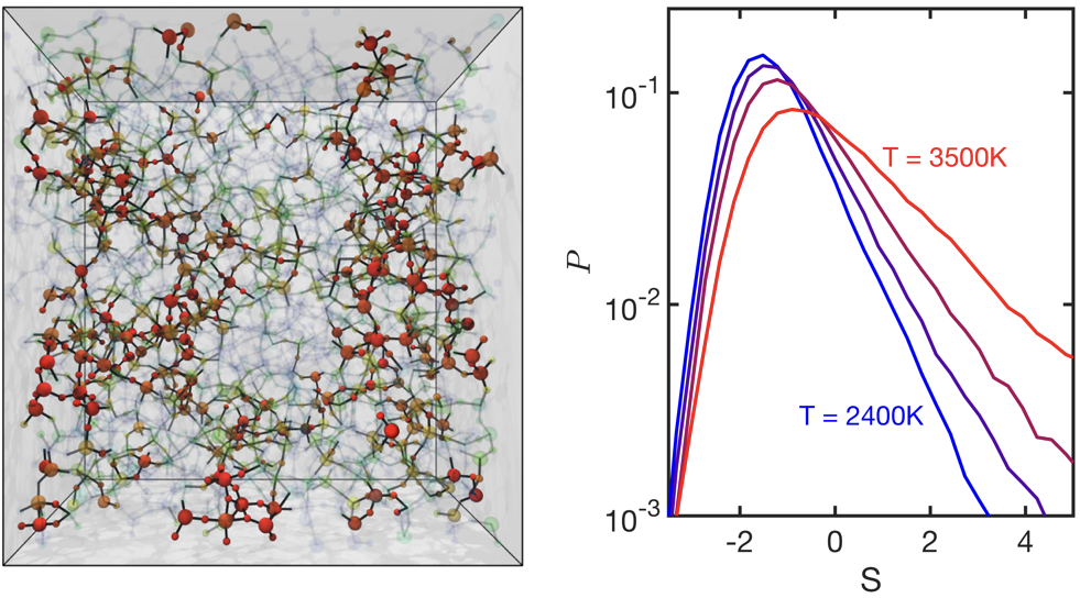
Figure 1: (a) A snapshot of the SiO₂ unit cell at 2500 K. Softness is represented on an opacity scale with $S\ll 0$ being transparent and $S\gg 0$ being opaque. (b) Distribution of softness, $P(S)$ at temperatures 2400 K, 2700 K, 3000 K, and 3500 K, with line types ranging from blue to red.

We examine the probability of rearrangement $P_{R}(S)$, given by the fraction of particles of softness $S$ that are rearranging at a given time step, averaged over time steps. The temperature-dependence of $P_{R}(S)$ at each $S$ was found to be Arrhenius for particles with spherically-symmetric interactions Schoenholz et al. (2016, 2017), for polymers made up of monomers with spherically-symmetric interactions plus anisotropic bonding along the polymer backbone Sussman et al. (2017) and aluminum atoms in polycrystals Sharp et al. (2018)). We find this to be true for SiO₂ as well (Fig. 2a), implying that the rearrangements in silica are governed by Arrhenius processes where the free energy barrier to rearrangement is decided by the local structure of the atoms (characterized by $S$). . This is surprising since SiO₂ behaves significantly differently at low and high temperatures. We fit $P_{R}(S)$ to the Arrhenius form:

$$P_{R}(S)=\mathrm{exp}(\Sigma(S)-\Delta E(S)/T),$$ (2)

where $\Sigma(S)$ and $\Delta E(S)$ are fitting constants for each $S$ and the free energy barrier is interpreted as $\Delta F(S)\equiv E(S)-T\Sigma(S)$. We plot $\Delta E(S)$, the energy barrier to rearrangement, and $\Sigma(S)$, the temperature-independent term, as a function of $S$ in Fig 2b.

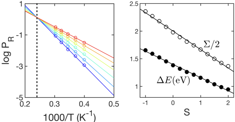
Figure 2: (a) Probabilities of rearrangement as a function of inverse temperature for six different softness values from $S\sim-1$ (blue) to $S\sim 2.75$ (red). Circles denote measurements from MD, solid lines are the corresponding Arrhenius fits. Vertical dashed line indicates the onset temperature ($\sim$ 4150 K). (b) Extracted energy barrier and prefactor from the Arrhenius fits in (a).

Given that the dynamics are Arrhenius at all temperatures, what causes the strong-to-fragile crossover as $T$ increases? To answer this question, we study how $S$ itself changes as a function of time. We begin by equilibrating the silica melt at 6000 K, and then rapidly lower the temperature to $T_{f}$. We then follow the system as it approaches equilibrium at fixed temperature and volume. In Fig 3(a), we show how the average softness of particles, $\langle S\rangle$ changes as a function of waiting time, $t_{w}$, following the temperature quench for several temperatures between 2400 K and 3100 K. It is interesting to note that the average softness, $\langle S\rangle$, of systems with different $T_{f}$ decays at the same rate until a system equilibrates; this was also observed for the Kob-Andersen glassformer Schoenholz et al. (2017). For systems that equilibrate within $10^{6}$ ps, we estimate $\langle S\rangle_{\mathrm{eq}}$by direct measurement. For systems that do not equilibrate within our simulation timescale, we investigate the functional form of $\langle S\rangle(t_{w})$. We find that it can approximated by a power law function of the form $\langle S\rangle(t_{w})=C\cdot t_{w}^{-\alpha}+\langle S\rangle_{\mathrm{eq}}$. By curve-fitting to the data shown in Fig. 3(a), we extrapolate to obtain $\langle S\rangle_{\mathrm{eq}}$ as a function of temperature. The results are shown in Fig. 3(b).

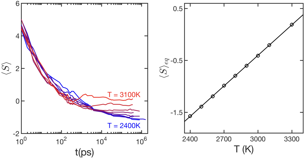
Figure 3: (a) Average softness as a function of waiting time at temperatures $T=2400$ K to 3100 K. The line-type/color scheme is the same as in Fig. 1. (b) Equilibrium softness values vs. T. The line is a fit to the equilibrium softness values.

The linear fit to $\langle S\rangle_{\mathrm{eq}}(T)$ is strikingly good. It shows that the average scale for the energy barriers encountered in liquid silica is linear in temperature, at least in the range that we have studied (2400 K - 6000 K). This linear behavior can be contrasted with the phenomenology of silica. At the low temperatures near 2400K, liquid silica behaves as a strong liquid, where the dynamics scale with temperature in an Arrhenius fashion Böhmer et al. (1993). As the temperature is increased, silica transitions into a fragile liquid Saika-Voivod et al. (2001).

To explore fragility vs. $T$ in terms of softness, we must relate $\langle S\rangle_{\mathrm{eq}}(T)$ to relaxation. In silica, relaxation is typically quantified by the diffusion constant, defined via the long-time behavior of the mean squared displacement,

$$\lim_{t\to\infty}\langle(r(t)-r(0))^{2}\rangle\sim Dt.$$ (3)

We now follow the considerable empirical evidence and assume that particles diffuse via discrete hops that occur intermittently compared with caged vibrations. We take the timescale for vibrations to be $\tau_{\mathrm{vib}}\approx 400$ fs. Thus, in a similar spirit to Niblett et al. (2016), we write

$$r(t)=\sum_{n=0}^{t/\tau_{\mathrm{vib}}}\Delta r_{n}+r(0)$$ (4)

where $\Delta r_{n}$ is the displacement during a hop that occurs (or does not occur) at a time $n\tau$.

To analyze Eq. (4), we make the additional approximation that hops are independent in time such that $\langle\Delta r_{i}\Delta r_{j}\rangle=\langle(\Delta r_{i})^{2}\rangle\delta_{ij}.$ While this does not hold exactly - especially when $i=j\pm 1$ - for events that do not occur in succession this approximation is reasonable Niblett et al. (2016). Moreover, we assume the system is in equilibrium so that $\langle(\Delta r_{i})^{2}\rangle=\langle(\Delta r_{0})^{2}\rangle=\langle(\Delta r)^{2}\rangle$. It follows that the diffusion constant is related to the hop statistics by

$$D\sim\langle(\Delta r)^{2}\rangle.$$ (5)

As we have hinted at above, Eq. (5) is difficult to analyze since $\Delta r$ contains contributions from both hopping and non-hopping particles. We therefore introduce $\langle(\Delta R)^{2}\rangle$ to be the average displacement of hopping particles. We may now introduce softness directly and rewrite Eq. (5) as

$$D\sim\langle(\Delta R)^{2}\rangle\int dSP(S)P_{R}(S).$$ (6)

Finally, we make the mean-field approximation and write, $D\sim\langle(\Delta R)^{2}\rangle P_{R}(\langle S\rangle_{eq})$. As has been noted in previous studies Schoenholz et al. (2016), $\langle(\Delta R)^{2}\rangle$ is only weakly temperature-dependent and so most of the temperature dependence should be contained in $P_{R}(\langle S\rangle_{eq})$.

Although we have significantly simplified the dynamics, we will see that this approximate framework suffices to explain the temperature dependence of silica. Combining the above arguments with the Arrhenius form of $P_{R}(S)$ we find,

$$\frac{1}{D(T)} \propto\frac{1}{P_{R}(\langle S\rangle_{\mathrm{eq}}(T))}$$ (7)

$$=\mathrm{exp}(\Delta E(\langle S\rangle_{\mathrm{eq}}(T))/T-\Sigma(\langle S\rangle_{\mathrm{eq}}(T))),$$ (8)

where $\Sigma(S)$ and $\Delta E(S)$ are given by the fits shown in Fig 2(b), and $\langle S\rangle_{\mathrm{eq}}(T))$ is given by the fit in Fig 3(a).

Since both $\Sigma(S)$ and $\Delta E(S)$ are approximately linear in the softness we can rewrite Eq. (8) as $\Sigma(S)=\Sigma_{0}+\Sigma_{1}S$ and $\Delta E(S)=E_{0}+E_{1}S$ respectively. As such, we can rewrite Eq. (8) as,

$$\frac{1}{D(T)}\propto\exp\left[\left(\frac{E_{0}}{T}-\Sigma_{0}\right)-\left(\frac{E_{1}}{T}-\Sigma_{1}\right)S\right].$$ (9)

Note that Eq. 9 predicts that the diffusivity is independent of softness at the temperature $T_{0}=E_{1}/\Sigma_{1}$; this is the onset temperature (vertical dashed line in Fig. 2(a). Finally, since $S$ depends linearly on temperature we can write $S=S_{0}+S_{1}T$ and so the temperature dependence of Eq. (8) is given by

$$\frac{1}{D(T)}\propto\exp\left[\frac{E_{0}-E_{1}S_{0}}{T}+\Sigma_{1}S_{1}T\right].$$ (10)

Thus we see that a crossover naturally emerges. When $\Sigma_{1}S_{1}T\gg(E_{0}-E_{1}S)/T$ we expect silica to exhibit non-Arrhenius relaxation while at lower temperatures we recover strong liquid behavior, as expected.

We plot Eq. 10 in Fig. 4 as a solid line. We note that the predicted $\frac{1}{D(T)}$ has a fragile-to-strong transition at approximately 3000 K. For a quantitative comparison, we also measure the inverse diffusivity of oxygen atoms in silica as a function of temperature, using the RMS displacement of the oxygen atoms, shown as red circles in Fig. 4. We used one fitting parameter to match the constant of proportionality in Eq. 10. Evidently our prediction based on $\langle S\rangle_{\mathrm{eq}}(T))$ predicts the diffusivity of the atoms remarkably well over the entire temperature range studied, spanning the strong-to-fragile crossover. Note that the solid line only extends up to the onset temperature, as local structure is not relevant to dynamics above the onset temperature, by definition Schoenholz et al. (2014).

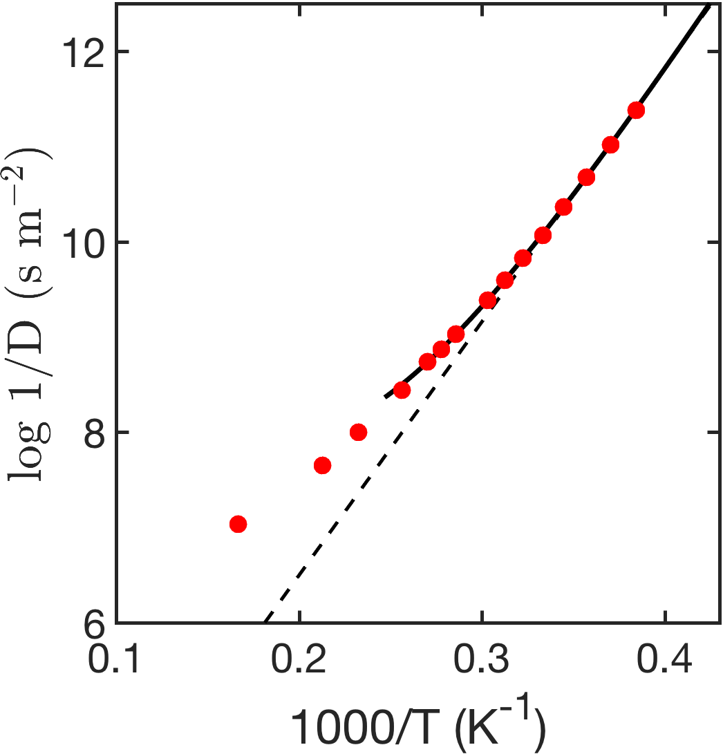
Figure 4: Inverse diffusivity vs. inverse temperature. Circles are measurements from MD simulations, and the solid line is our prediction based on $\langle S\rangle_{\mathrm{eq}}$ and the Arrhenius form. Note that the prediction is made only for temperatures below the onset temperature. The dashed line denotes the strong scaling, to reveal the strong-to-fragile crossover.

In conclusion, we have shown that a simple model based on softness quantitatively predicts the temperature-dependence of relaxation in supercooled BKS silica. The same reasoning predicts the temperature-dependence of relaxation in a fragile glassformer, the Kob-Andersen model. Note that although the method of calculating softness is the same for different systems, the actual definition of softness is based on the classification hyperplane, which depends on the system. Nevertheless, it has been shown that the emergent properties of softness in systems below yield exhibit commonality Cubuk et al. (2017a). Here we have shown that commonality in the emergent properties of softness extends even to the temperature-dependence of relaxation in glassformers of arbitrary fragility. The fact that relaxation in both fragile and strong systems is well-described by the same simple reasoning in terms of average softness implies that softness provides a unifying framework for relaxation dynamics in glassy liquids. The difference in fragility arises from the differing dependences of average softness on temperature. For silica, the average softness is well-approximated as linear in $T$. For the Kob-Andersen system, the average softness is well-approximated by $\langle S\rangle=c_{0}-c_{1}/T$. Our results shift the theoretical challenge from understanding fragility in glassforming liquids to understanding the temperature-dependence of a purely structural (static) quantity, $\langle S\rangle$.

Machine learning has already emerged as a promising tool for materials design Bassman et al. (2018); Sendek et al. (2020); Cheon et al. (2018); Hoyt et al. (2019) as well as building conceptual models Hoffmann et al. (2019); Rajak et al. (2019a, b). The ability to find predictive, compressed representations of physical data using machine learning becomes truly useful to theoretical physics if we can use those representations to build new models. This approach has the potential to be particularly useful for systems that are far out of equilibrium and/or disordered and/or that exhibit nonlinear response, where we cannot use statistical mechanics to bridge the gap between microscopic models and macroscopic behavior. In such situations, machine learning may provide a way of connecting microscopic information to collective behavior.

I Methods

I.1 Machine Learning Model

As descriptors of local structure, we use structure functions that were used to predict the dynamics of Lennard-Jones particles and granular pillars Cubuk et al. (2015). These structure functions are closely related and are inspired by the symmetry functions that were proposed by Behler and Parrinello Behler and Parrinello (2007). While these descriptors have been described in previous work in detail Cubuk et al. (2015); Schoenholz et al. (2016, 2017); Cubuk et al. (2017a); Sharp et al. (2018); Ivancic and Riggleman (2019); Ma et al. (2019); Freitas and Reed (2020), we briefly introduce them here.

Radial structure functions are given by,

$$G(k;\mu) =\sum_{i}\mathrm{e}^{-(r_{ik}-\mu)^{2}/L^{2}}$$ (11)

which provides information about the radial density at distance $\mu$ from particle $k$, where $r_{ik}$ is the distance between particles $i$ and $k$. We choose the range of $\mu$ to be between 0 and 7 Å. The parameter $L$ is the size of the window in radius, which is set to $L=0.2$ Å.

Angular structure functions are given by,

$$\Psi(k;\xi,\lambda,\zeta) =\sum_{i,j}\mathrm{e}^{-\left(r_{ik}^{2}+r_{jk}^{2}+r_{ij}^{2}\right)/\xi^{2}}\left(1+\lambda\cos\theta_{kij}\right)^{\zeta}$$ (12)

where $\xi$, $\lambda$, and $\zeta$ are variables that characterize angular structure functions; $\theta_{kij}$ is the angle made between particles $k$, $i$, and $j$. These functions count the number of large and small bond angles within a distance $\xi$ of particle $k$. By varying $\lambda=\pm 1$, we can count large or small bond angles. $\zeta$ parameter controls the angular resolution of the structure functions. We identify rearrangements using the $p_{hop}$ measure, with a time window of 4 ps, and a cutoff of $p_{hop}=0.6s$. The optimal C parameter of the linear SVM was found to be 1 by cross-validation. As mentioned in the main text, the training set and test set accuracies were both found to be 86% when both radial and angular structure functions are used. When we restrict our model to only use radial structure functions, the prediction accuracy goes down to 79%.

I.2 Identifying Rearrangements

To identify rearrangements we use the $p_{\text{hop}}$ metric that was first proposed by Candelier et. al. Candelier et al. (2010) and has since been used extensively to identify rearrangements in amorphous materials Smessaert and Rottler (2013); Schoenholz et al. (2016). To construct $p_{\text{hop}}$, first a timescale $t_{R}=4$ ps is chosen to be commensurate with the timescale for rearrangements to take place in the system. Then two time intervals are defined as $A_{t}=[t-t_{R}/2,t]$ and $B_{t}=[t,t+t_{R}/2]$. For each particle $i$, $p_{\text{hop}}$ can be written as,

$$p_{\text{hop}}(t)\sqrt{\langle(r_{i}-\langle r_{i}\rangle_{B})^{2}\rangle_{A}\langle(r_{i}-\langle r_{i}\rangle_{A})^{2}\rangle_{B}}$$ (13)

where $\langle\rangle_{A}$ and $\langle\rangle_{B}$ are averages over the $A$ and $B$ interval respectively. When a particle is trapped in a cage, $\langle r_{i}\rangle_{A}\approx\langle r_{i}\rangle_{B}$ and $p_{\text{hop}}$ is equal to the scale of fluctuations about the cage center. However, when a particle has undergone a rearrangement, the means will shift and $p_{\text{hop}}$ will be exhibit a peak. The size of this peak will be commensurate with the size of the rearrangement.

II acknowledgments

We would like to thank Austen Angell and Evan Reed for helpful discussions.

References

- Angell (1985) C. Angell, Relaxations in complex systems 3 (1985).
- Angell (1991) C. Angell, Journal of Non-Crystalline Solids 131, 13 (1991).
- Salmon and Zeidler (2013) P. S. Salmon and A. Zeidler, Physical Chemistry Chemical Physics 15, 15286 (2013).
- Saika-Voivod et al. (2001) I. Saika-Voivod, P. H. Poole, and F. Sciortino, Nature 412, 514 (2001).
- Geske et al. (2016) J. Geske, B. Drossel, and M. Vogel, AIP Advances 6, 035131 (2016).
- Kob and Andersen (1994) W. Kob and H. C. Andersen, Phys. Rev. Lett. 73, 1376 (1994).
- Schoenholz et al. (2016) S. S. Schoenholz, E. D. Cubuk, D. M. Sussman, E. Kaxiras, and A. J. Liu, Nature Physics 12, 469 (2016).
- Schoenholz et al. (2017) S. S. Schoenholz, E. D. Cubuk, E. Kaxiras, and A. J. Liu, Proceedings of the National Academy of Sciences 114, 263 (2017).
- Landes et al. (2019) F. P. Landes, G. Biroli, O. Dauchot, A. J. Liu, and D. R. Reichman, arXiv preprint arXiv:1906.01103 (2019).
- Sussman et al. (2017) D. M. Sussman, S. S. Schoenholz, E. D. Cubuk, and A. J. Liu, Proceedings of the National Academy of Sciences 114, 10601 (2017).
- Van Beest et al. (1990) B. Van Beest, G. J. Kramer, and R. Van Santen, Phys. Rev. Lett. 64, 1955 (1990).
- Horbach and Kob (1999) J. Horbach and W. Kob, Physical Review B 60, 3169 (1999).
- Vollmayr and Kob (1996) K. Vollmayr and W. Kob, Berichte der Bunsengesellschaft für physikalische Chemie 100, 1399 (1996).
- Plimpton (1995) S. Plimpton, J. Comp. Phys. 117, 1 (1995).
- Thompson et al. (2009) A. P. Thompson, S. J. Plimpton, and W. Mattson, The Journal of chemical physics 131, 154107 (2009).
- Brown et al. (2011) W. M. Brown, P. Wang, S. J. Plimpton, and A. N. Tharrington, Computer Physics Communications 182, 898 (2011).
- Brown et al. (2012) W. M. Brown, A. Kohlmeyer, S. J. Plimpton, and A. N. Tharrington, Computer Physics Communications 183, 449 (2012).
- Bitzek et al. (2006) E. Bitzek, P. Koskinen, F. Gähler, M. Moseler, and P. Gumbsch, Phys. Rev. Lett. 97, 170201 (2006).
- Cubuk et al. (2017a) E. Cubuk, R. Ivancic, S. Schoenholz, D. Strickland, A. Basu, Z. Davidson, J. Fontaine, J. Hor, Y.-R. Huang, Y. Jiang, et al., Science 358, 1033 (2017a).
- Sharp et al. (2018) T. A. Sharp, S. L. Thomas, E. D. Cubuk, S. S. Schoenholz, D. J. Srolovitz, and A. J. Liu, Proceedings of the National Academy of Sciences 115, 10943 (2018), http://www.pnas.org/content/115/43/10943.full.pdf .
- Cubuk et al. (2015) E. D. Cubuk, S. S. Schoenholz, J. M. Rieser, B. D. Malone, J. Rottler, D. J. Durian, E. Kaxiras, and A. J. Liu, Phys. Rev. Lett. 114, 108001 (2015).
- Behler and Parrinello (2007) J. Behler and M. Parrinello, Phys. Rev. Lett. 98, 146401 (2007).
- Khaliullin et al. (2011) R. Z. Khaliullin, H. Eshet, T. D. Kühne, J. Behler, and M. Parrinello, Nat. Mater. 10, 693 (2011).
- Behler (2015) J. Behler, International Journal of Quantum Chemistry 115, 1032 (2015).
- Artrith et al. (2011) N. Artrith, T. Morawietz, and J. Behler, Physical Review B 83, 153101 (2011).
- Artrith and Behler (2012) N. Artrith and J. Behler, Physical Review B 85, 045439 (2012).
- Artrith et al. (2013) N. Artrith, B. Hiller, and J. Behler, physica status solidi (b) 250, 1191 (2013).
- Artrith and Urban (2016) N. Artrith and A. Urban, Computational Materials Science 114, 135 (2016).
- Cubuk et al. (2017b) E. D. Cubuk, B. D. Malone, B. Onat, A. Waterland, and E. Kaxiras, The Journal of chemical physics 147, 024104 (2017b).
- Onat et al. (2018) B. Onat, E. D. Cubuk, B. D. Malone, and E. Kaxiras, Physical Review B 97, 094106 (2018).
- Cortes and Vapnik (1995) C. Cortes and V. Vapnik, Mach. Learn. 20, 273 (1995).
- Chang and Lin (2011) C.-C. Chang and C.-J. Lin, ACM Transactions on Intelligent Systems and Technology 2, 27 (2011).
- Fan et al. (2008) R.-E. Fan, K.-W. Chang, C.-J. Hsieh, X.-R. Wang, and C.-J. Lin, Journal of machine learning research 9, 1871 (2008).
- Kob et al. (2002) W. Kob, M. Nauroth, and F. Sciortino, Journal of non-crystalline solids 307, 181 (2002).
- Freitas and Reed (2020) R. Freitas and E. J. Reed, Nature Communications 11, 1 (2020).
- Gumbel (1935) E. J. Gumbel, in Annales de l’institut Henri Poincaré, Vol. 5 (1935) pp. 115–158.
- Böhmer et al. (1993) R. Böhmer, K. Ngai, C. A. Angell, and D. Plazek, The Journal of chemical physics 99, 4201 (1993).
- Niblett et al. (2016) S. Niblett, V. de Souza, J. Stevenson, and D. Wales, The Journal of chemical physics 145, 024505 (2016).
- Schoenholz et al. (2014) S. S. Schoenholz, A. J. Liu, R. A. Riggleman, and J. Rottler, Phys. Rev. X 4, 031014 (2014).
- Bassman et al. (2018) L. Bassman, P. Rajak, R. K. Kalia, A. Nakano, F. Sha, J. Sun, D. J. Singh, M. Aykol, P. Huck, K. Persson, et al., npj Computational Materials 4, 1 (2018).
- Sendek et al. (2020) A. D. Sendek, G. Cheon, M. Pasta, and E. J. Reed, The Journal of Physical Chemistry C 124, 8067 (2020).
- Cheon et al. (2018) G. Cheon, E. D. Cubuk, E. R. Antoniuk, L. Blumberg, J. E. Goldberger, and E. J. Reed, The journal of physical chemistry letters 9, 6967 (2018).
- Hoyt et al. (2019) R. A. Hoyt, M. M. Montemore, I. Fampiou, W. Chen, G. Tritsaris, and E. Kaxiras, Journal of chemical information and modeling 59, 1357 (2019).
- Hoffmann et al. (2019) J. Hoffmann, Y. Bar-Sinai, L. M. Lee, J. Andrejevic, S. Mishra, S. M. Rubinstein, and C. H. Rycroft, Science advances 5, eaau6792 (2019).
- Rajak et al. (2019a) P. Rajak, A. Krishnamoorthy, A. Nakano, P. Vashishta, and R. Kalia, Physical Review B 100, 014108 (2019a).
- Rajak et al. (2019b) P. Rajak, R. K. Kalia, A. Nakano, and P. Vashishta, MRS Advances 4, 1109 (2019b).
- Ivancic and Riggleman (2019) R. J. Ivancic and R. A. Riggleman, Soft matter 15, 4548 (2019).
- Ma et al. (2019) X. Ma, Z. S. Davidson, T. Still, R. J. Ivancic, S. Schoenholz, A. Liu, and A. Yodh, Physical review letters 122, 028001 (2019).
- Candelier et al. (2010) R. Candelier, A. Widmer-Cooper, J. K. Kummerfeld, O. Dauchot, G. Biroli, P. Harrowell, and D. R. Reichman, Phys. Rev. Lett. 105, 135702 (2010).
- Smessaert and Rottler (2013) A. Smessaert and J. Rottler, Phys. Rev. E 88, 022314 (2013).