Compact galaxies and the size-mass galaxy distribution from a colour-selected sample at $0.04<z<0.15$ supplemented by $ugrizYJHK$ photometric redshifts

Abstract

The size-mass galaxy distribution is a key diagnostic for galaxy evolution. Massive compact galaxies are potential surviving relics of a high-redshift phase of star formation. Some of these could be nearly unresolved in SDSS imaging and thus not included in galaxy samples. To overcome this, a sample was selected from the combination of SDSS and UKIDSS photometry to $r<17.8$. This was done using colour-colour selection, and then by obtaining accurate photometric redshifts (photo-z) using scaled flux matching (SFM). Compared to spectroscopic redshifts (spec-z), SFM obtained a 1-sigma scatter of 0.0125 with only 0.3% outliers ($|\Delta\ln(1+z)|>0.06$). A sample of 163 186 galaxies was obtained with $0.04<z<0.15$ over $2300\,{\rm deg}^{2}$ using a combination of spec-z and photo-z. Following Barro et al., $\log\Sigma_{1.5}{}={}\log{}M_{*}-1.5\log r_{50,\mathrm{maj}}$ was used to define compactness. The spectroscopic completeness was 76% for compact galaxies ($\log\Sigma_{1.5}>10.5$) compared to 92% for normal-size galaxies. This difference is primarily attributed to SDSS ‘fibre collisions’ and not the completeness of the main galaxy sample selection. Using environmental overdensities, this confirms that compact quiescent galaxies are significantly more likely to be found in high-density environments compared to normal-size galaxies. By comparison with a high-redshift sample from 3D-HST, $\log\Sigma_{1.5}$ distribution functions show significant evolution, with this being a compelling way to compare with simulations such as EAGLE. The number density of compact quiescent galaxies drops by a factor of about 30 from $z\sim{}2$ to $\log{}(n/\mathrm{Mpc}^{-3}){}={}-5.3\pm{}0.4$ in the SDSS-UKIDSS sample. The uncertainty is dominated by the steep cut off in $\log\Sigma_{1.5}$, which is demonstrated conclusively using this complete sample.

1 Introduction

The galaxy population of the local Universe is very different to its ancestral population ten billion years ago at $z\sim 2$. One of the most striking changes is the transformation of the radially small massive galaxies seen at high redshift to the larger and more diffuse red galaxies seen today. Multiple observations indicate that a high proportion of galaxies at $z>2$ are already ‘red and dead’ as well as unusually small for their mass relative to local red galaxies (e.g., Daddi et al. 2005; Trujillo et al. 2007). A quintessential high-redshift quiescent galaxy, or ‘red nugget’, has a stellar mass ($M_{*}$) of $\sim 10^{11}\mathrm{M}_{\odot}$ and a half-light radius of $\sim 1\,\mathrm{kpc}$ (Buitrago et al., 2008; van Dokkum et al., 2008; Damjanov et al., 2009).

Considering the demographics in more detail, at $z\sim 2$ almost half of the massive ($M_{*}>10^{10}\mathrm{M}_{\odot}$) galaxy population are both quiescent (e.g. Cimatti et al. 2004; Kriek et al. 2006) and radially smaller than quiescent galaxies locally (Daddi et al., 2005; Trujillo et al., 2007; Longhetti et al., 2007; Buitrago et al., 2008; Barro et al., 2013). The red nuggets at $z\sim 2.3$ measure 5–6 times smaller than the median size of low-redshift samples (Shen et al., 2003; Lange et al., 2015) for the same mass (van Dokkum et al., 2008). These observations have posed a significant challenge for theories of galaxy evolution.

In a hierarchical structure formation scenario, red nuggets should evolve into the most massive ellipticals in the local Universe (e.g., Trujillo et al. 2007). An early proposed mechanism for this evolution involved an adiabatic expansion of stellar systems in response to a significant mass loss from their inner regions. This mass expulsion is thought to be driven by means of stellar winds or/and quasars and to increase the effective radius as $R_{e}\propto M^{-1}$ (Fan et al., 2008; Damjanov et al., 2009; Fan et al., 2010; Ragone-Figueroa & Granato, 2011). However, the amount of the stellar mass loss is too small to explain the size evolution (Damjanov et al., 2009). Compact massive galaxies are already quiescent in terms of star-formation activity at high $z$ and they do not seem to possess sufficient gas to increase their stellar component significantly (Bezanson et al., 2009).

A natural hierarchical explanation for this radial growth would involve major mergers ($\sim 1$:1 mass ratio) building the red sequence from the high-redshift compacts to the local red giant ellipticals. However, major mergers result in equal growth of both mass and radius (Naab et al., 2009); they shift galaxies along the high-redshift mass-radius relation rather than towards the low-redshift relation (see also Boylan-Kolchin et al. 2006). Major mergers are effectively ruled out of consideration for this reason, and because ‘wet’ (star-forming) mergers would leave a signature in the stellar density profiles of galaxies that is not seen (Szomoru et al., 2012).

The current view for explaining the size-mass evolution is that a series of minor mergers together with accretion of a stellar envelope have combined to build either local elliptical galaxies or massive spiral/S0 galaxies (Hopkins et al., 2010; Sonnenfeld et al., 2014; van Dokkum et al., 2014; Graham et al., 2015; Buitrago et al., 2017). Progenitor bias has also been invoked in explaining the apparent size evolution of the red galaxy population as a class (e.g. Szomoru et al. 2012; Carollo et al. 2013). In fact, as noted by Barro et al. (2013), both paths must operate: an early formation of massive compact galaxies that become quenched and then grow via minor mergers (Naab et al., 2009; Hilz et al., 2012), and a late-arrival path in which larger star-forming galaxies build mass and then form extended quenched galaxies (Barro et al., 2013).

It has long been recognised that local massive ellipticals generally have old stellar populations with little recent star formation. However, they could still have undergone significant evolution due to mergers unless they are compact. The stochastic nature of merging processes suggests that a non-negligible number of quiescent massive compact galaxies at each redshift between 2 and 0 should be unaltered, old and compact ‘relics’ (Trujillo et al., 2014). Quantifying the number density of these massive compact relics in the present-day universe is thus an important constraint on galaxy formation models (Quilis & Trujillo, 2013; Ferré-Mateu et al., 2017), in addition to relics being local analogs of the high-redshift red nuggets (Saulder et al., 2015; Yıldırım et al., 2017; Martín-Navarro et al., 2019).

Valentinuzzi et al. (2010) searched for and found a population of compact galaxies in local $0.04<z<0.07$ clusters using mass and surface mass density lower limits. Poggianti et al. (2013) showed that the fraction of these ‘superdense’ galaxies was 3–4 times higher in groups with high velocity dispersion ($>500$ km/s) compared to the field. This means that it requires large volumes using blind surveys in order to sample compact galaxies in high-density environments. Saulder et al. (2015) searched the Sloan Digital Sky Survey (SDSS) for compact quiescent galaxies, using a lower limit on galaxy velocity dispersion ($>300$ km/s) in addition to an upper limit on size ($\la 2$ kpc), finding only 76 galaxies at $0.05<z<0.3$. Even these are not as extreme as the high redshift red nuggets. Using deeper imaging in the Galaxy And Mass Assembly (GAMA) survey regions, Buitrago et al. (2018) found 22 massive compact galaxies ($\log M_{*}>10.9$) with number density $\sim 10^{-6}\,\mathrm{cMpc}^{-3}$ at $z<0.3$. Various authors have quantified the evolution in the number density of compact galaxies (e.g. Barro et al. 2013; Cassata et al. 2013; van Dokkum et al. 2015; Tortora et al. 2016; Charbonnier et al. 2017), for $\log M_{*}>10$ or higher limits, for quiescent/star-forming galaxies, and with various definitions of compactness (e.g. Gargiulo et al. 2016; Lu et al. 2019). The number density of compact quiescent galaxies peaks around $z\sim 1$–2.

There is some concern that local galaxy surveys could be missing extremely compact galaxies due to mis-identification with stars in the input catalogue. For example, for the SDSS main galaxy sample, $r<17.77$ mag, a profile separator is used for galaxy selection (Strauss et al., 2002). Without this, there would be about ten times as many stars as galaxies for this magnitude limit. Liske et al. (2006) spectroscopically identified all sources over $1.14\,{\rm deg}^{2}$ to $B<20$ mag for the Millenium Galaxy Catalogue (MGC). They estimated that about 1% of galaxies in the MGC input catalogue were mis-identified as stars. The volume probed in the $\sim 1\,{\rm deg}^{2}$ region, however, was not sufficient to search for massive compact galaxies. Taylor et al. (2010) considered the selection of galaxies in SDSS, which includes cuts against saturation, spectroscopic fiber crosstalk, and the concentration of light. All of these characteristics predispose compact galaxies to exclusion by the SDSS automated data pipeline for spectroscopic selection. Taylor et al. concluded that the SDSS completeness should be $\ga 75$% for the types of compact galaxies seen at high redshift but maybe as low as $\sim 20$% for the smallest galaxies.

The aim of this paper is to determine the local number densities of compact galaxies using a complete sample. This is enabled by star-galaxy separation using colours and photometric redshifts based on 9-band photometry from the combination of SDSS (York et al., 2000) and the UKIRT Infrared Deep Sky Survey (UKIDSS, Lawrence et al. 2007). The sample selection and photometric redshifts are described in § 2 and § 3. The results of the size-mass relations and distributions are presented and discussed in § 4, and a summary is presented in § 5. Size tests and images of compact galaxies are presented in the Appendix. We assume a flat $\Lambda$CDM cosmology with $H_{0}=70{\rm\,km\,s^{-1}\,Mpc^{-1}}$ and $\Omega_{m,0}=0.3$.

2 Sample selection

2.1 Data

Sources were selected from the SDSS DR14 database with $r<17.8$ ($r$-band extinction-corrected Petrosian magnitude) covering five separate sky areas as shown in Table 1 (from tables PhotoPrimary and, where available, SpecObj). This approximately matched the UKIDSS Large Area Survey (LAS) sky coverage. No restrictions were applied based on photometric flags or star-galaxy separation. This produced a catalog of 3.38 million sources covering $2664\,{\rm deg}^{2}$.

Table 1: Sky areas. RA and DEC limits for selection of sources from catalogs. The areas were chosen to approximately match UKIDSS LAS coverage.

RA range (deg.) DEC range (deg.) note 125 to 238 $-2$ to 15 LAS main region 114 to 128  18 to 30 190 to 210  22 to 36 240 to 250  22 to 32 $>309.2$ or $<58.6$ $-1.26$ to 1.26 Stripe 82

Sources were selected from the UKIDSS database lasYJHKsource table, which provides combined data for the LAS survey. The magnitude limits were $Y<18.4$ or $J<18.1$ with magnitude types petromag, apermag3 or apermag4. These limits were a magnitude fainter than expected for any typical type of galaxy given the SDSS $r$-band limit. The aim was to be inclusive at this stage. This produced a catalog of 15.28 million sources.

Sources were selected from the GAIA DR2 gaia_source table over the areas defined in Table 1. This produced a catalog 12.02 million sources, of which, 687 471 have a GAIA $G$-band magnitude brighter than 15.

2.2 Masking radii around GAIA sources

The SDSS main galaxy sample (Strauss et al., 2002) excluded sources for which the saturated flag was set. This was to remove artifacts that are caused by light either diffracted or scattered from bright stars. Without resorting to this flag, it is instead possible to remove these types of artifacts by masking the sky area around selected stars. These stars are, of course, uncorrelated with the galaxy distribution and there is no bias in trimming the catalogue using this method.

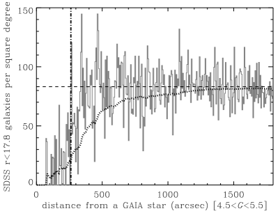
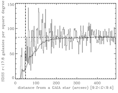
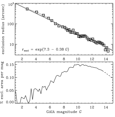
The exclusion radius around GAIA stars was empirically determined using the spectroscopically-confirmed galaxy sample from SDSS. To do this, the sky density of confirmed galaxies around each star was measured in bins of separation and GAIA magnitude of the star. Two examples of this are shown in Figure 1. The radius at which the sky density (within the radius) is 25% of the expected sky density was determined. This was chosen as visually this is the radius at which the impact of the stellar stray light becomes negligible. Figure 2 shows the resulting exclusion radii versus the GAIA magnitude.

Figure 1: Examples of SDSS spectroscopically-confirmed galaxy sky densities around GAIA stars. The grey solid-line shows the sky density histogram. The dashed line shows the mean sky density away from the stars. The dotted line shows the cumulative sky density (accounting for sky area). The vertical dash-dot line show the radius at which the cumulative sky density is 25% of the mean. This corresponds to the empirical estimate of the exclusion radius.

Figure 2: Top panel: exclusion radius versus GAIA $G$ magnitude. The squares and dotted line represent the results from the empirical determination for each bin (examples in Fig. 1). The solid grey line shows a fit to the these points, with the parameters and equation annotated. Lower panel: percentage of excluded area including all stars and using exclusion-radius values from the fit. The solid line shows the magnitude range used for this project, while the dashed line shows a small extension to 15th magnitude.

2.3 Trimming the area

The sample selection requires UKIDSS data and since the initial query did not take account of the exact coverage, significant adjustment to the area was needed. In particular, there is a requirement for $Y$, $J$ and $K$ data, and the UKIDSS coverage was defined with the criteria that valid photometry exists in all these bands. At the same time, there are genuine SDSS galaxies without a UKIDSS catalogue match and these should not be rejected. Therefore the SDSS sample was trimmed by area and not by match criteria.

The SDSS master sample was trimmed in area using the following:

• Seven polygons were defined where there was no UKIDSS coverage and sources within these polygons were removed.

• A $6^{\prime}\times 6^{\prime}$ grid was defined and sources in grid areas without any UKIDSS coverage were removed.

• One polygon was defined where there was no SDSS spectroscopy and sources within this polygon were removed.

• Sources in areas with $g$-band Galactic extinction greater than 0.4 were removed.

• Sources in the masked areas around $G<13.5$ GAIA stars were removed (§ 2.2). Note GAIA sources include galaxies but no spectroscopically-confirmed SDSS galaxies had a GAIA aperture magnitude brighter than 14.5 in the sample. Therefore, 13.5 is a safe limit that even compact galaxies would not be excluded.

This produced a catalog of 2.48 million sources covering $2300\,{\rm deg}^{2}$.

2.4 Colour-colour galaxy selection

In order to avoid using a profile separator for star-galaxy separation, galaxies were selected using a combination of SDSS and UKIDSS colours. To do this, we considered two colour-colour diagrams: $J-K$ versus $g-i$ and $Y-K$ versus $g-z$. These show the cleanest separation between galaxies and stars, while also not requiring matched-aperture or matched-profile photometry between UKIDSS and SDSS. For UKIDSS, we used apermag4 ($2.8^{\prime\prime}$-diameter aperture) and for SDSS, we used psf and Petro magnitudes. The UKIDSS aperture was chosen to provide accurate colours for stars and galaxies, $2.8^{\prime\prime}$ is more than twice the typical seeing of $<1^{\prime\prime}$ (Dye et al., 2006). The SDSS psf magnitudes provide the most precise colours for point sources whereas Petro magnitudes provide the best unbiased colours for extended sources.

The basic method is to obtain a quadratic fit to the stellar locus of the UKIDSS colour as a function of the SDSS colour over a suitable range, with clipping of the function beyond that range. The galaxy selection is then defined as galaxies with UKIDSS colour greater than 0.2 above the function value.

The $J-K$ separator is given by

$$\Delta_{\rm sg,jk,gi}=J_{\rm AB}-K_{\rm AB}-f_{\rm locus}(g-i)$$ (1)

with the locus function as per Baldry et al. (2010). For this paper, we determined the locus function for $Y-K$ versus $g-z$ colours using spectrosopcially-confirmed stars and with point-spread function (PSF) magnitudes for the SDSS colours. This additional separator is given by

$$\Delta_{\rm sg,yk,gz}=Y_{\rm AB}-K_{\rm AB}-f^{\prime}_{\rm locus}(g-z)$$ (2)

where

$$f^{\prime}_{\rm locus}(x)=\begin{array}[]{l}-0.8297\\ -1.04+0.74x-0.13x^{2}\\ 0.0128\end{array}\mbox{~{}for~{}}\begin{array}[]{l}x<0.3\\ 0.3<x<2.8\\ x>2.8\end{array}$$ (3)

Figure 3: Colour-colour distributions for spectroscopically-confirmed galaxies and stars. The distributions are shown by contours and points. The blue lines show the stellar locus fits. The green lines show the selection boundaries for galaxies, 0.2 above the locus function.

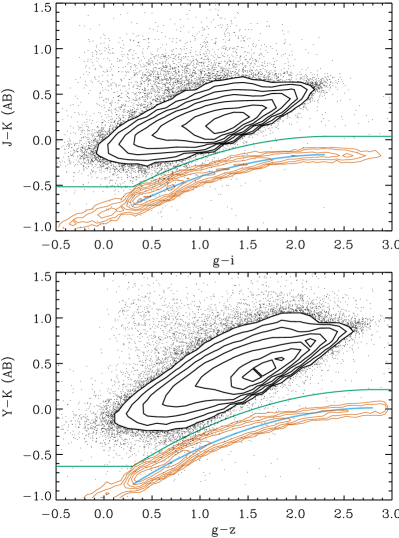
Figure 3 shows the two colour-colour diagrams used to distinguish stars from galaxies. Note that when determining the $\Delta$ values for the selection, the bluer of SDSS PSF and SDSS Petrosian magnitudes are used for each source. This is in order to be inclusive toward galaxy selection (where the Petrosian colours could be different from the PSF colours). The colour-only galaxy selection is then given by

$$0.2<\Delta_{\rm sg,jk,gi}<3\mbox{~{}~{}~{}\&~{}~{}~{}}0.2<\Delta_{\rm sg,yk,gz}<3$$ (4)

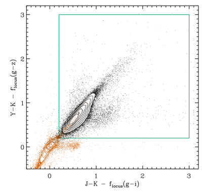
with the high cuts used to exclude some cases of photometric measurement problems. Figure 4 shows these selection boundaries with the distributions of $\Delta_{\rm sg,yk,gz}$ versus $\Delta_{\rm sg,jk,gi}$ for stars and galaxies.

Figure 4: Boundaries in the $\Delta$ values used to select galaxies. The distributions are shown for spectroscopically-confirmed galaxies (black contours and points) and stars (orange contours and points).

The colour-colour selection results in 225 634 sources. Of these, 198 123 have an associated reliable SDSS redshift, with 99.2%, 0.3% and 0.5% classified as a galaxy, star and quasar, respectively (a galaxy being defined to have $0.002<z<0.4$ or by spectral class from the SDSS pipeline). This demonstrates the high purity of this selection.

2.5 Additional selections

The above selection is not complete because of the reliance on SDSS-UKIDSS matching, and this can miss extended sources where the UKIDSS aperture position is offset or undefined. In addition, the method of trimming the area to UKIDSS $Y$, $J$ and $K$ coverage is not perfect. Additional sources with SDSS photometry but no UKIDSS match were selected using the SDSS star-galaxy profile separator,

$$\Delta_{\rm sg,prof}=r_{\rm model}-r_{\rm psf}\mbox{~{}~{}~{},}$$ (5)

satisfying the following criteria:

$$\Delta_{\rm sg,prof}>0.5\mbox{~{}~{}~{}\&~{}~{}~{} not {saturated} ~{}~{}~{}\&~{}~{}~{}}\mu_{r,50}<24.5\mbox{~{}~{}~{},}$$ (6)

where $\mu_{r,50}$ is the Petrosian half-light surface brightness. These criteria selected 15 309 sources.

On top of the UKDSS-SDSS and SDSS-only selections, 4533 sources that were galaxy targets in DR7 and 169 spectroscopically-confirmed galaxies, but not otherwise selected, were included. Including all four selections, this results in 245 645 sources, of which 86.1% have redshifts from SDSS and 0.2% from 2MRS (Huchra et al., 2012). This leaves 13.7% without spectroscopic redshifts (spec-z).

3 Photometric redshifts from scaled flux matching (SFM)

The above combined selection (§ 2) primarily selects galaxies. However, 1.0% of the sources are spectroscopically-confirmed stars (kept in for testing purposes) and a significant fraction of those without spec-z are stars. This is because there are about 10 times as many stars as galaxies at these magnitudes ($r<17.8$), and finding any nearly unresolved galaxies is like ‘looking for a needle in a haystack’. To refine the search further, we use a photometric redshift (photo-z) technique that identifies sources with galaxy-like fluxes (beyond that already considered with the colour-colour selection). In addition, redshifts are needed to estimate luminosities and physical sizes.

Photo-z methods are generally divided into two classes: template fitting (e.g. Babbedge et al. 2004; Brammer et al. 2008) and empirical. When there are many sources with reliable spec-z covering the colour and magnitude space of a sample, which is the case for this SDSS-UKIDSS sample, empirical methods should be more accurate (Koo, 1999). Here, we note that empirical methods can be further divided into: (a) predictive modelling, for example, using neural networks (Firth et al., 2003) or analytical functions (Connolly et al., 1995; Sedgwick et al., 2019a); and (b) photometric-property matching, typically using colours and a magnitude (Baldry et al., 2006; Beck et al., 2016). In the latter method, a source’s photo-z is obtained by the distribution of spec-z for galaxies with similar properties. Here, we use scaled flux matching (SFM). This is similar to colour matching except that it works in linear flux space with the advantage that it can naturally deal with missing data, low S/N measurements (Sedgwick et al., 2019b) or, more generally, different errors in each band.

3.1 General method

For each source $i$ and band $k$, the uncertainty in the flux is given by:

$$\sigma_{i,k}^{2}=\sigma_{i,k,\mathrm{P}}^{2}+(a_{k}f_{i,k})^{2}$$ (7)

where $\sigma_{i,k,\mathrm{P}}$ is the Poisson/counting or linear error, $a_{k}$ is the band-dependent fractional error, and $f_{i,k}$ is the flux. If the Poisson error is not well determined, then a band-dependent value could be used. The flux measurements and flux uncertainties are also corrected for Galactic extinction.

For each source, the fluxes are matched to the matching-set galaxy ($j$) fluxes with chi-squared defined as:

$$\chi^{2}_{i,j}=\sum_{k}\frac{(f_{i,k}-n_{i,j}f_{j,k})^{2}}{\sigma_{i,k}^{2}}$$ (8)

where $n_{i,j}$ is the usual best-fit normalization when scaling a model to fit data points with errors (obtained from solving $\mathrm{d}\chi^{2}/\mathrm{d}n=0$):

$$n_{i,j}=\frac{\sum_{k}f_{j,k}f_{i,k}/\sigma_{i,k}^{2}}{\sum_{k}f_{j,k}^{2}/\sigma_{i,k}^{2}}\mbox{~{}~{}~{}.}$$ (9)

Note that no uncertainty is applied to the matching-set fluxes in the calculaton of chi-squared.

The reliability weight of the match is then given by:

$$w_{i,j}=\exp(-\chi^{2}_{i,j}/2)\,W_{j}$$ (10)

where $W_{j}$ is any additional weight assigned to galaxy $j$ of the matching set. This could be, for example, to downweight redshift bins that are well populated. Importantly, $w_{i,j}$ is set to zero where $i$ and $j$ refer to the same galaxy. This is so the photo-z of the matching-set galaxies are independent of their spec-z.

These weights could then be used to estimate a probability distribution function (PDF) if desired (see Wolf 2009). In general, this method is accurate if the matching set is large and the galaxies for which photo-z are desired are within the covered range of spectral-energy distribution (SED) type and redshifts. A characterization of the PDF is then given by the weighted mean and standard deviation. The weighted mean of the redshift variable is given by:

$$\zeta_{i,\mathrm{phot}}=\frac{\sum_{j}w_{i,j}\zeta_{j,\mathrm{spec}}}{\sum_{j}w_{i,j}}\mbox{~{}~{}~{}where~{}~{}~{}}\zeta=\ln(1+z)\>.$$ (11)

Noting that $\zeta$ (zeta) is the appropriate quantity to use when dealing with redshift measurements and errors (Baldry, 2018).

The initial estimate of the uncertainty (nominal error) is given by:

$$\zeta_{i,\mathrm{err}}^{2}=\left(\frac{\sum_{j}w_{i,j}\zeta_{j,\mathrm{spec}}^{2}}{\sum_{j}w_{i,j}}\>-\>\zeta_{i,\mathrm{phot}}^{2}\right)\frac{N_{i,\mathrm{eff}}}{N_{i,\mathrm{eff}}-1}$$ (12)

which is the weighted standard deviation multiplied by a correction factor to obtain the sample standard deviation. The effective number of measurements for reliability weights is given by

$$N_{i,\mathrm{eff}}=\frac{\left(\sum_{j}w_{i,j}\right)^{2}}{\sum_{j}w_{i,j}^{2}}\mbox{~{}~{}~{}.}$$ (13)

3.2 Specific implementation

SDSS modelmag values were converted to fluxes (Lupton et al., 1999) in units of nanomaggies (log-flux zeropoint of 22.5 mag, AB system; Blanton et al. 2005). For photo-z measurements, modelmag fluxes were chosen because they provide the highest S/N for point and extended sources. UKIDSS apermag4 (1.4^′′-radius aperture) magnitudes were converted to fluxes in the same units (Vega to AB magnitude conversion was taken to be $+0.63,+0.94,+1.38,+1.90$ for $Y,J,H,K$, Hill et al. 2011; though we note this is not necessary for SFM).

Despite the fact that the SDSS and UKIDSS fluxes were not obtained using the same types of apertures, the SFM method could still be used to calculate photo-z. However, an improvement can be made by scaling the SDSS fluxes to better match the UKIDSS fluxes prior to using SFM. This allows for a greater number of potential low $\chi^{2}$ matches. For each source, the $i$-band flux within a $1.4^{\prime\prime}$ circular aperture was estimated using both the de-Vaucouleurs and exponential profile fits (§ 4.4.5.5 of Stoughton et al. 2002) and combined with weights fracdev and $1-$fracdev, respectively (analogous to cmodel, Abazajian et al. 2004). This is effectively a (PSF-deconvolved) circular-aperture flux estimated using a galaxy profile model. The ratio between this flux and the $i$-band modelmag was determined, and used to scale the SDSS fluxes, for each source. After this process, both the SDSS and UKIDSS fluxes represent similar size apertures. It is not ideal aperture-matched photometry but it is sufficient for SFM because it is an empirical matching technique.

The choice of flux errors is important as it sets the relative weights between the best fitting matching-set galaxies. By guidance from nominal limiting magnitudes and by trial and error, the linear errors, in place of Poisson errors, were taken to be $(0.84,0.54,0.72,1.08,4.44,3.0,3.0,3.0,3.0)$ nanomaggies for $(u,g,r,i,z,Y,J,H,K)$. The fractional errors ($a_{k}$) were taken to be 0.05 in the $u$-band and 0.02 in all the other bands. The $u$-band was down weighted by this because of the signicantly larger spread in these magnitudes compared to a median SDSS magnitude for each source. This spread primarily reflects variations in star-formation rate (SFR) with less constraint on photo-z.

For any missing measurements (mostly where no UKIDSS match was available), the error is set to a extremely large value and the flux to zero (i.e. to give no effect on normalization or chi-squared). In addition, for each source the magnitudes (SDSS and UKIDSS, separately) were compared to a median value, and any measurements outside a large tolerance were set as if missing. Thus, some bad measurements are accounted for and do not affect the photo-z determination.

The matching set was chosen as a subset of the sample with all the following criteria: zwarning$=0$, spectroscopic classification as a galaxy, valid photometric measurements in all nine bands, and $0.002<\zeta<0.5$. The matching-set galaxies were binned in $\zeta$ with binsize of 0.002. The weights $W_{j}$ for all ($n_{\rm bin}$) galaxies in a bin were set to $100/n_{\rm bin}^{\alpha}$ with $\alpha=0.5$ with a maximum weight of 20 (when $n_{\rm bin}\leq 25$). The choice of $\alpha=0.5$ is a compromise between equal weight to all galaxies ($\alpha=0$) and effectively setting equal weight to all bins ($\alpha=1$). The number of matching-set galaxies was 194 183.

3.3 Selecting reliable galaxy redshifts

In order to assess the reliability of the photo-z, the number of matches with $\chi^{2}<30$ is considered, hereafter $C_{30}$, along with the nominal error ($\zeta_{i,\mathrm{err}}$, Eq. 12). Figure 5 shows the distribution in $C_{30}$ in the upper panel. Taking only photo-z measurements where there is also a reliable spec-z, the lower panel indicates the fraction of sources spectroscopically classified as stars and the fraction where there is a significant redshift offset $|\Delta\ln(1+z)|>0.08$ between photo-z and spec-z. To eliminate poor photo-z and stars from the sample, only sources with $6<C_{30}<100000$ were set as having reliable photo-z.

Figure 5: Upper panel: histogram in $C_{30}$ of the photo-z measurements. Lower panel: fraction of sources (stacked bar chart) classified as stars (orange) and fraction with a redshift offset between the spec-z and photo-z given by $|\Delta\ln(1+z)|>0.08$ (blue). The range used to select reliable photo-z is shown by the dashed line in both panels.

Figure 6: Upper panel: histogram in $\zeta_{i,\mathrm{err}}$ of the photo-z measurements. Lower panel: fraction of sources (stacked bar chart) with a redshift offset between the spec-z and photo-z given by $|\Delta\ln(1+z)|>0.08$ (blue), and fraction with offset between 0.06 and 0.08 (pink). The range used to select reliable photo-z is shown by the dashed line in both panels. The sample used for this figure was selected to have $6<C_{30}<100000$, i.e., within the reliable range shown in Fig. 5.

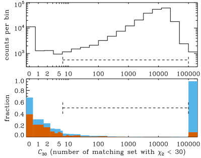
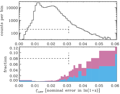
Figure 6 shows the distribution in $\zeta_{i,\mathrm{err}}$. As expected, the fraction of photo-z outliers generally increases with the nominal error estimate. To select sources with reliable photo-z, we additionally applied the criteria $\zeta_{i,\mathrm{err}}<0.031$. In total, 93.1% of the 245 645 sources from Section 2 have reliable photo-z; and 98.3% of spec-z confirmed galaxies. Thus most of the 6.9% of the sample without reliable photo-z are expected to be stars. Of the reliable photo-z sample, only 1 in 1000 are spec-z confirmed stars; and of those with photo-z $>0.04$, only 1 in 3000. Thus without using any photometric profile information, these have a very low stellar contamination.

3.4 Redshift accuracy

Figure 7 shows a plot of spec-z versus photo-z for the reliable photo-z sample. The correlation is good with no obvious bias (considering that the contours represent logarithmically-spaced number densities). The 68th percentile ($\sigma_{68}$) of $|\Delta\ln(1+z)|$ is 0.0125, and the 95th percentile ($\sigma_{95}$) is 0.030.

Figure 7: Distribution of photo-z versus spec-z for sources with reliable photo-z and spectroscopic zwarning$=0$. The solid-line contours show logarithmically spaced densities with a factor of two between each contour. 98% of the data are represented by the contours, and 2% by the points. The dashed lines show the limits of $|\Delta\ln(1+z)|=0.06$ (99.7% of the data).

These SFM ($ugrizYJHK$) redshifts were compared with the empirical photo-z for SDSS from Beck et al. (2016). The latter were determined using ‘local linear regression’ for redshift as a function of the $r$-band magnitude and four colours ($u-g$, $g-r$, $r-i$, $i-z$). For the Beck et al. photo-z to spec-z difference, $\sigma_{68}=0.0144$ and $\sigma_{95}=0.0357$ using a comparison sample of photo-z for which the Beck et al. analysis defines as reliable (photoerrorclass$=1$). Thus, the SFM photo-z have a 25-30% reduction in the error variance compared to the Beck et al. photo-z. This is because of the addition of the near-IR data rather than the method, which is a similar empirical method using a $\chi^{2}$ matching formalism. In any case, the Beck et al. photo-z were not determined for SDSS sources photometrically classified as stars. Therefore we only use the SFM photo-z that also do not have a magnitude prior.

3.5 Final galaxy sample selection

For the 245 645 sources from § 2, redshifts are assigned with the following priority: reliable SDSS spec-z, 2MRS, and then reliable photo-z (§ 3.3), with 86.1%, 0.2%, and 9.4%, respectively. The remainder are assumed to be stars or quasars. Redshifts are converted from the heliocentric to the CMB frame, used hereafter. The galaxy sample selection for this study is then $0.04<z<0.15$.

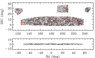
Compact galaxy candidates were visually inspected and 27 sources whose photometry was significantly affected by scattered light (missed by the masking procedure) or a bright neighbour were rejected. In addition, 138 sources with GAIA photometry that had $\mathrm{S/N}>5$ for their parallax measurement or $\mathrm{S/N}>10$ for their proper motion were rejected. The latter cut was set high because there were many obviously extended sources that had S/N between 5 and 10, some of which may be star-galaxy blends but in other cases it was not clear. After the redshift limits and these cuts, a sample of 163 186 sources remained. Figure 8 shows the sky positions of a subset of the sample.

Figure 8: Sky positions of the galaxy sample with $17.3<r<17.5$ demonstrating the $ugrizYJHK$ coverage ($2300\,{\rm deg}^{2}$) from SDSS and UKIDSS. The black dots represent galaxies with spec-z and the red dots with photo-z.

4 Results and discussion

4.1 Stellar masses

Stellar masses ($M_{*}$) were determined for the spec-z and photo-z sample using the the method of Sedgwick et al. (2019a) (updated from Bryant et al. 2015) such that

$$\log M_{*}=-0.4i+0.4{\cal D}+f(\mathrm{z})+g(\mathrm{z})(g-i)_{\rm obs}$$ (14)

where $i$ is the $i$-band cmodel magnitude, ${\cal D}$ is the distance modulus, and $(g-i)_{\rm obs}$ is the observed colour using Petrosian magnitudes. This effectively folds the mass-to-light ratio and k-correction into the same formula. These magnitude types were chosen as cmodel represents the best estimate of the total flux derived from profile fits, while Petrosian magnitudes provide the best unbiased estimate of galaxy colours. The functions $f(\mathrm{z})$ and $g(\mathrm{z})$ are calibrated to a stellar-population fitted set of stellar masses. In this case, the functions were calibrated using the GAMA survey photometry and products (Baldry et al., 2018) with the stellar masses from the magphys code (da Cunha et al., 2008) applied by Driver et al. (2016). These masses were used in order to be consistent with the high-z comparison sample.

The functions used in this paper are given by $f(z)=1.008-3.531z+21.64z^{2}-35.28z^{3}$ and $g(z)=0.8132+3.304z-30.26z^{2}+55.60z^{3}$. The calibration is valid over the range $0<z<0.35$. The stellar initial mass function (IMF) assumed was the Chabrier (2003) IMF.

We note that dynamical modelling using resolved spectroscopy (Cappellari et al., 2012; Posacki et al., 2015) and detailed stellar population analysis (Conroy & van Dokkum, 2012; La Barbera et al., 2013) have suggested that there is a bottom-heavy IMF in early-type galaxies that have high velocity dispersion. This is relevant for massive and/or compact galaxies. For example, Ferré-Mateu et al. (2017) modelled the spectra of two compact galaxies using steep IMF slopes. However, Collier et al. (2018) showed that the mass obtained using gravitational lensing for four low-redshift ($z<0.07$) massive ellipticals was consistent with a Kroupa (2001) IMF. Strong lensing of these galaxies is dominated by their stellar mass (Smith & Lucey, 2013) and therefore is an accurate constraint on stellar mass-to-light ratios. Regardless of the variation or not of the IMF between galaxies, it is appropriate to assume a universal IMF for distribution functions or relationships involving stellar mass because the extra mass, if any, for some galaxies has little impact on broadband photometry and, for transparency and simplicity, the stellar mass can be considered as a ‘modified luminosity’. This is particularly the case here because we only use $g$- and $i$-bands to estimate the stellar mass. Stellar masses obtained assuming a Kroupa IMF (Salpeter IMF) are about 0.05 dex (0.25 dex) higher than using the Chabrier IMF (Collier et al., 2018).

The stellar mass approximation, above, uses observed colour. To define red galaxies, we use

$$(u-r)_{\rm adj}=u-r-4.5\ln(1+z)\>.$$ (15)

This approximates the $k$-and-evolution correction for dividing the red and blue sequences of galaxies at a rest-frame $u-r\sim 2$.

Specific star formation rates (SSFRs) were obtained for the sample from the SDSS table galSpecExtra. These were derived from spectral emission lines (Brinchmann et al., 2004) with aperture corrections using photometry (Salim et al., 2007). For sources without a match, e.g. with photo-z only, the nearest SFM matching-set galaxy was used for the SSFR. This provided SSFR measurements for 98.6% of galaxies with $\log M_{*}>10$. Red galaxies were defined using $(u-r)_{\rm adj}>2.0$ while quenched galaxies were defined using $\log(\mathrm{SSFR/yr}^{-1})<-11.2$ (or using the red galaxy definition for the 1.4% without SSFR measurements) for this $z<0.15$ sample.

4.2 Half-light radii

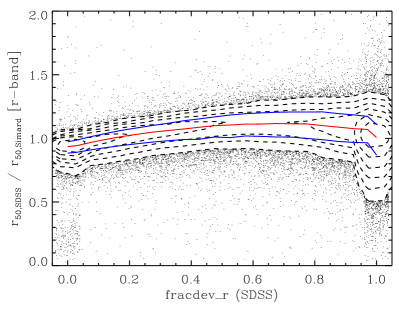
Various half-light radii ($r_{50}$) are provided for SDSS. The SDSS pipeline computes Petrosian $r_{50}$ (circular), de Vaucolueurs and exponential profile fits (elliptical) (Stoughton et al., 2002). Only the profile fits take account of the PSF. The SDSS pipeline “also takes the best-fit exponential and de Vaucouleurs fits in each band and asks for the linear combination of the two that best fits the image” (Abazajian et al., 2004). This provides a coefficient (clipped between zero and one), called fracdev ($f_{\rm dev}$), that gives the relative flux contribution of the de Vaucouleurs fit, with $1-f_{\rm dev}$ giving the contribution of the exponential fit. This ‘composite model’ is effectively a non-simultaneous fit of the two profile functions because the profiles are fitted separately before being combined. In addition, Simard et al. (2011) provides bulge plus disk simultaneous fits, and Sersic fits for SDSS galaxies with spec-z, using gim2d (Simard et al., 2002). These are provided for the $g$- and $r$-bands.

Since the Simard et al. fits are not provided for sources without spec-z, or for the $i$-band, we used the half-light radii from SDSS with a weighted geometric average of the two models for each band:

$$\log r_{50,\mathrm{maj}}=f_{\rm dev}\log r_{\rm dev}+(1-f_{\rm dev})\log r_{\rm exp}\mbox{~{}~{}~{}.}$$ (16)

Figure 9 shows a comparison between the the radii from these non-simultaneous fits with the simultaneous fits (de Vaucolueurs bulge plus exponential disk) of Simard et al.. There is generally good agreement with 93% of galaxies within 0.1 dex, and 98.5% within 0.2 dex. The geometric weighted mean for SDSS agreed marginally better with the comparison sample than the linear weighted mean.

Figure 9: Comparison between the half-light radii determined using the SDSS profile fits (weighted average) with the radii from Simard et al. (2011). The dashed contours and points show the bivariate distribution, of the galaxy sample, in the ratio between the radii measurements versus fracdev_r, which is determined by the SDSS pipeline. (Note jitter has been added to fracdev_r to spread out the data at 0 and 1.) The red and blue solid lines show the median, 16th and 84th percentiles of the ratios binned in fracdev_r. For the whole sample, 93% of the galaxies have measurements differing by less than 0.1 dex (ratios between 0.79 and 1.26).

The final $r_{50,\mathrm{maj}}$ we used was taken as the mean between the $r$ and $i$-band. This was to increase the fidelity, ensuring that compact galaxies had to have small fitted radii in two bands, while avoiding the bluer $g$-band that crosses the 4000Å break at $z>0$ and the $z$-band which is of lower S/N. The mean rest-frame effective wavelength of the $r$- and $i$-bands is $\sim$6000–6500Å for $0.04<z<0.15$. For a few sources, half-light radii were clipped to a minimum of $0.3^{\prime\prime}$. In total, there were 34 unresolved sources with mean radius $<0.35^{\prime\prime}$ and that were photometrically classified as a star by the SDSS pipeline. Of the 18 that had estimated stellar masses $\log M_{*}>10$, all but one had log SSFR $>-10$. This sample is of interest as candidate compact starbursts but has no significance for the number densities of the compact quiescent population. Note Taylor et al. (2010) used a minimum of $0.75^{\prime\prime}$ for the $z$-band sizes, however, we find that reasonable agreement between the Simard et al. (2011) and pipeline half-light radii, and between $i$- and $r$-bands, extends to lower values. This is testament to the accuracy with which the PSF is measured and accounted for in the galaxy profile fitting. See Appendix for further comparisons.

4.3 Size-mass distribution

Figure 10 shows the size-mass distribution of the SDSS-UKIDSS selected sample. Following Barro et al. (2013), we define a projection in the size-mass distribution that runs perpendicular to the quiescent size-mass relation at high masses. This is given by

$$\log\Sigma_{1.5}=\log(M_{*}/\mathrm{M}_{\odot})-1.5\log(r_{50,\mathrm{maj}}/\mathrm{kpc})\mbox{~{}~{}~{}.}$$

Thus $\Sigma_{1.5}$ has units of $\mathrm{M}_{\odot}\mathrm{kpc}^{-1.5}$ and uses physical half-light radius. Compact galaxies are shown with circles in the figure that have $\log\Sigma_{1.5}>10.5$ (sample images are shown in Fig. 19). This represents only 0.12% of the sample at $\log M_{*}>10$. Note we prefer to use the major axis to define radii and $\Sigma_{1.5}$ because cicularization of effective radii is strongly inclination dependent (Devour & Bell, 2017).

Figure 10: Size-mass distribution for the galaxy sample ($0.04<z<0.15$). The contours and points represent the majority of the galaxy sample, while the circles represent galaxies with $\log\Sigma_{1.5}>10.5$ (black with spec-z and orange with photo-z). The dashed line shows $\log\Sigma_{1.5}=9.85$, which is the median for the quiescent population at $\log(M_{*}/\mathrm{M}_{\odot})>10$. The red dotted lines show the two-power-law fits from Lange et al. (2015) for the $r$- and $i$-bands $r_{50,\mathrm{maj}}$ with the early-type division using Sersic index and $u-r$. The grey dotted box shows the ultra-compact massive galaxy (UCMG) selection with a $r_{50,\mathrm{maj}}<2.0$ cut.

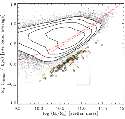
The orange circles in Fig. 10 represent the 26% of the compact galaxy sample that have photo-z only. For compact galaxies, there is a significantly larger fraction with photo-z compared to the full sample. This demonstrates a bias against compact galaxies in the SDSS spectroscopic sample. Figure 11 shows the spectroscopic and target completeness as a function of $\log\Sigma_{1.5}$ ($r<17.75$ to minimise the issue of photometric scatter across the 17.77 selection boundary between SDSS data reduction versions). The target completeness, in this paper, is the fraction of sources that were selected as targets for SDSS spectroscopy regardless of whether a spectrum was obtained. The spectrocopic (target) completeness is 91.6% (99.4%) in the normal $\log\Sigma_{1.5}$ range (8.8–10.3). This drops to 75.8% (96.7%) for $\log\Sigma_{1.5}>10.5$. This means that the majority of the bias against compact galaxies is due to ‘fibre collisions’ and not the SDSS photometric selection. Fibre collisions were caused by the restriction of how close fibres could be placed on the spectroscopic plate (Stoughton et al., 2002). The bias arises because compact galaxies are more likely to be found in proximity to other SDSS galaxies (Trujillo et al., 2014) (§ 4.6).

Figure 11: Completeness as a function of $\log\Sigma_{1.5}$. The solid line shows the spectrosopic completeness of the sample, while the dashed line shows the SDSS target completeness i.e. the fraction of galaxies that were part of the SDSS main galaxy sample, primarily. Also shown are the fraction of red galaxies [$(u-r)_{\rm adj}>2.0$] and quenched galaxies [$\log({\rm SSFR/yr}^{-1})<-11.2$].

The fraction of red galaxies and quenched galaxies as a function of $\log\Sigma_{1.5}$ is also shown in Figure 11. The red fraction is higher than the quenched fraction for less compact galaxies. This is because the estimate of SSFR takes account of internal dust attenuation whereas the $u-r$ colour does not. In other words, some dusty star forming galaxies appear as red but not as quenched. The red/quenched fraction rises from less than 0.2 at $\log\Sigma_{1.5}\sim 9.0$ to 0.95 at $\sim 10.2$. This range is where the majority of galaxies are distributed. For compact galaxies ($\log\Sigma_{1.5}>10.5$), the red/quenched fraction drops below 0.85. This is due to a small population of quasars and starburst galaxies, for which, the SDSS half-light radii likely do not represent the overall stellar population within each galaxy.

4.4 High-z comparison

In order to compare the distribution functions from the SDSS-UKIDSS sample at $z\sim 0.1$ to high redshift, we used the 3D-HST survey data. These are five fields with near-IR grism spectra (Brammer et al., 2012) and photometry from HST primarily from the CANDELS treasury programme (Grogin et al., 2011). The construction of the photometric catalogues, including space and ground-based imaging, is described in Skelton et al. (2014). The science area (use_phot=1) of the combined fields is $0.249\,{\rm deg}^{2}$. The sources were assigned photo-z, ground-based spec-z or grism redshifts (Momcheva et al., 2016).

Structural parameters using Sersic models were determined for the sources by van der Wel et al. (2012) in the near-IR F160W ($H$) and F125W ($J$) bands. These included half-light radii and profile-integrated magnitudes. Stellar masses and SSFR were determined by Driver et al. (2018) using magphys. For this paper, the stellar masses were corrected for the difference between the F160W magnitude (Skelton et al., 2014) used in the magphys fitting and the Sersic F160W magnitude. F125W was used if F160W was not available ($<0.5$% of sources). The same procedure was used in van der Wel et al. (2014), except here we use the magphys stellar masses. Selecting galaxies with $0.5<z<2.5$, $\log M_{*}>10$, use_phot$\,=1$, and rejecting poor fits visually checked by van der Wel et al. (2014), produced a volume-limited sample of 9757 galaxies (over $4.8\times 10^{6}\,\mathrm{cMpc}^{3}$).

The half-light radii were obtained using the F160W band ($>99.5$% of sources), which has a pivot wavelength of 15400Å. This matches the rest-frame wavelength used for the low-redshift sample at $z\sim 1.5$. At higher redshifts, the rest-frame wavelength drops below 6000Å and thus the measured radii are potentially affected more significantly by younger stellar populations. This is mitigated by the fact that the colour gradients in galaxies are close to zero at $z\sim 2$–2.5 (Suess et al., 2019). Therefore, measurements in F160W in the high-z sample can be reasonably compared to the low-z measurements without significant concern regarding the dependence of radii on rest-frame wavelength.

Star-forming galaxies form a ‘main sequence’ in SSFR versus stellar mass that evolves with redshift (Noeske et al., 2007; Salim et al., 2007; Pearson et al., 2018; Popesso et al., 2019). Therefore, we define ‘quenched’ using a dividing line that evolves with redshift such that

$$\log({\rm SSFR}_{\rm divide}/{\rm yr}^{-1})\>=\>-11.2+1.2\ln(1+z)\>,$$ (17)

which corresponds to $-10.4$ at $z=1$ and $-9.7$ at $z=2.5$ [$-11.2+2.76\log(1+z)$]. This dividing line is about 1 dex below the SSFR versus redshift of the main sequence for $\log M_{*}>10$ galaxies.

4.5 Distribution functions

The total volume covered by the SDSS-UKIDSS sample is $54.6\times 10^{6}\,\mathrm{cMpc}^{3}$. This is only a volume-limited sample for $\log M_{*}\ga 10.9$. To determine distribution functions including galaxies less massive than this, 1/Vmax weighting was used (Eales, 1993). Distribution functions were then obtained by summing 1/Vmax in bins. For the high-z comparison sample, Vmax was the same for all galaxies in a given redshift range.

For the SDSS-UKIDSS sample, the maximum luminosity distance ($D_{L}$) that a galaxy, of the same type and luminosity, could be seen at and remain within the flux limit is given by

$$5\log(D_{L,\mathrm{max}})=5\log(D_{L,\mathrm{obs}})+17.8-r_{\rm Petro}+dK$$ (18)

where $dK$ accounts for the difference in the $k$-correction between the observed and maximum redshifts. For the purposes of this paper, sufficient accuracy was obtained with $dK$ set to zero. Then, from $D_{L,\mathrm{max}}$, the maximum redshift ($z_{\mathrm{max}}$) was determined for each galaxy. These $z_{\mathrm{max}}$ values were clipped to lie between a lower limit as a function of stellar mass, that was determined using the 1st percentiles in mass bins, and $z=0.15$, the redshift limit of the sample. Vmax is then given by the comoving volume between 0.04 and $z_{\mathrm{max}}$. At $\log M_{*}=10.0$, Vmax is about $5\times 10^{6}\,\mathrm{cMpc}^{3}$ for the least luminous galaxies ($z_{\mathrm{max}}\approx 0.07$), which are quenched galaxies. Thus the volume covered is larger than, or comparable to, the high-z comparison sample for all types of galaxies with $\log M_{*}>10$.

Figure 12 shows the galaxy stellar mass functions (GSMFs) for the SDSS-UKIDSS sample and for the high-z comparison split into three redshift bins. This demonstrates the trend that most of the highest mass galaxies ($\log M_{*}>11$) have been in place since $z\sim 2$ with more growth in number density occurring at lower masses (Davidzon et al., 2013; Muzzin et al., 2013; Mortlock et al., 2015; Huertas-Company et al., 2016; Wright et al., 2018; Kawinwanichakij et al., 2020). Kawinwanichakij et al. noted that the near absence of observed evolution in the number density of $\log M_{*}>11$ galaxies does not mean no mass growth. This is because stellar mass loss from late-stage stellar evolution could be compensated by mass growth from dry mergers or residual star formation. They estimated an upper limit of 0.16 dex for this mass growth of supermassive quiescent galaxies from $z=1.0$ to 0.4.

Figure 12: Galaxy stellar mass functions. The hatched regions represent the Poission counting uncertainties ($\pm\sigma$).

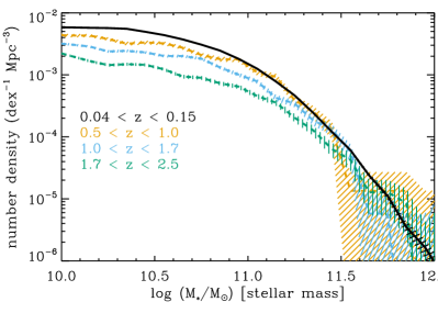
Size-mass distributions of the high-z sample are shown in figure 5 of van der Wel et al. (2014). In this paper, in order to demonstrate the evolution of the size-mass distribution in comparison to the SDSS-UKIDSS sample, we computed the distribution functions in $\log\Sigma_{1.5}$. In other words, this represents the number density of galaxies running perpendicular to the high-mass quiescent relation. Such a representation is suggested by the analysis of Barro et al. (2013). Figure 13 shows the $\log\Sigma_{1.5}$ distribution functions for the SDSS-UKIDSS sample and three high-z redshift bins for: (a) $\log(M_{*}/\mathrm{M}_{\odot})>10.0$, (b) quenched galaxies with the same mass limit, and (c) quenched galaxies with $\log(M_{*}/\mathrm{M}_{\odot})>10.9$.

Figure 13: $\log\Sigma_{1.5}$ distribution functions. The hatched regions represent the Poisson counting uncertainties ($\pm\sigma$). Upper panel (a): for all galaxies with $\log(M_{*}/\mathrm{M}_{\odot})>10.0$. Middle panel (b): for quenched galaxies. Lower panel (c): for supermassive quenched galaxies ($\log(M_{*}/\mathrm{M}_{\odot})>10.9$).

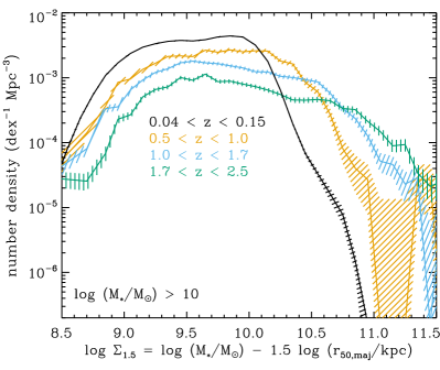
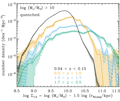
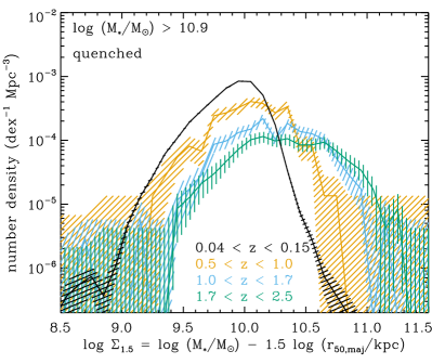
The evolution in the $\log\Sigma_{1.5}$ distribution functions (Fig. 13) is far more striking than the GSMF evolution (Fig. 12). The high $\log\Sigma_{1.5}$ cutoff becomes sharper and moves to lower values as the galaxy population evolves (from high to low redshift). At the same time, there is an increase in number density of the less compact galaxies ($\log\Sigma_{1.5}\la 10$). The pattern is similar for all three selections with narrowing of the functions for the quenched galaxies, and the supermassive ($\log(M_{*}/\mathrm{M}_{\odot})>10.9$) quenched galaxies.

This supports the picture of Barro et al. (2013) (their figure 6): size growth due to minor mergers (Naab et al., 2009; Hilz et al., 2012) for compact quenched galaxies that primarily formed at $z\ga 2$, and galaxies with normal sizes quenching at all these epochs. In this way, the $\log\Sigma_{1.5}$ distribution cutoff at high values becomes steeper. In this paper, we have demonstrated this by using a rigorously complete low-redshift galaxy selection for compact sources, and we also used the major axis for the half-light radii. Note that the increase of half-light radii caused by minor merger growth cannot be entirely due to addition of light at large radii. This was demonstrated by van Dokkum et al. (2014) who showed that the number density of high-mass-core galaxies, with $\log M_{*}>10.5$ within the central kpc of each galaxy, decreased from high to low redshift. This could be explained by a small amount of stellar-evolution mass loss from the core leading to adiabatic expansion.

In summary, compact quiescent galaxies can grow primarily through minor mergers that increase a galaxy’s mass and size. The size growth is a combination of adding mass to the envelope (Huang et al., 2013) and dynamical friction causing the core to expand (Naab et al., 2009). The mass increase can be compensated by mass loss from stellar evolution, and the core can also grow marginally through adiabatic expansion (van Dokkum et al., 2014). It should also be noted that compact galaxies can accrete a disk becoming early-type spirals (Gao & Fan, 2020), and then in some cases becoming low-redshift S0 galaxies (Graham et al., 2015; de la Rosa et al., 2016; Deeley et al., 2020). No doubt there is more than one path to galaxy growth given the stochastic nature of hierarchical assembly. Gao & Fan (2020) estimated, based on a spectral and structural analysis of SDSS galaxies, that about 15% of compact quiescent galaxies become spirals with a massive bulge with the remaining growing through dry minor mergers to become massive early types.

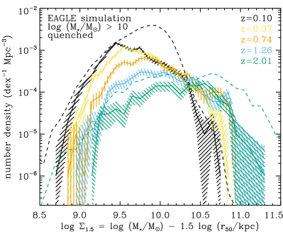
The evolution of the size-mass distribution of galaxies can be examined using cosmological-scale hydrodynamical simulations. Furlong et al. (2017) found good agreement for the size-mass evolution in the EAGLE simulation compared to the van der Wel et al. (2014) observational measurements. In all cases of $z=2$ compact galaxies identified in the simulation, stars formed at high redshift migrated to larger radii at $z=0$ (Furlong et al., 2017). For some of these galaxies, further growth occurred by mergers and star formation. Wellons et al. (2015) looked at the formation of supermassive compact galaxies at $z=2$ in the Illustris simulation, finding that they could be formed by gas-rich mergers at $z<4$ or by assembly at early times when the universe was much denser.

To examine the EAGLE simulation in terms of the $\log\Sigma_{1.5}$ distribution functions, we obtained data for five snapshots (different redshifts), four that matched the midpoints of the low- and high-z comparison measurements plus one intermediate redshift, from the $10^{6}\,\mathrm{cMpc}^{3}$ reference simulation box (McAlpine et al., 2016). Total stellar masses were defined in spheres of radius 30 kpc around each galaxy, with half-mass radii also defined in 3D (Furlong et al., 2017). Figure 14 shows the distribution functions from the simulation using these definitions of $M_{*}$ and $r_{50}$ for massive quenched galaxies using the SSFR cut of Eq. 17. There are clear quantitative differences compared to the observational data: a lower number density at all redshifts; and a lack of ultra-compact galaxies at high redshift that is not unexpected given the gravitational softening length of 0.7 kpc (Schaye et al., 2015). There is however strikingly good qualitative agreement. Crain et al. (2015) note that it is important for hydrodynamical simulations to match the observed size-mass relation otherwise simulations can end up with unrealistically compact low-z galaxies. While the EAGLE reference simulation was calibrated to the low-z relation, it was not to the high-z relations, and therefore this qualitative agreement is a success of the model.

Figure 14: $\log\Sigma_{1.5}$ distribution functions using the EAGLE hydrodynamical simulation. These are shown with solid lines, while the hatched regions represent the Poisson counting uncertainties ($\pm\sigma$). The dashed lines show the observational measurements that are the lowest and highest redshift bins from the middle panel of Fig. 13.

The distribution functions in Fig. 13 clearly demonstrate the number density evolution without the need to define a compact sample. Nevertheless, there is interest in the number density of compact galaxies that have largely evolved passively since high redshift. Figure 15 shows the evolution in the number density of compact galaxies with $\log\Sigma_{1.5}>10.5$ (cf. Barro et al. 2014 and Gu et al. 2020 use a limit of 10.45 with circularized radii). To estimate the uncertainty, the number densities were also determined using cuts at 10.4 and 10.6. The number density of low-redshift compact galaxies depends significantly on the cut since it is on the steep part of the $\log\Sigma_{1.5}$ distribution function, and this is the dominant uncertainty. The evolutionary trend is clear though with a peak at $z\sim 2$ and a steep decline in the number density towards low redshift (Cassata et al., 2013; van der Wel et al., 2014). The $z\sim 0.1$ number density of compact quenched galaxies from this study is $\log(n/\mathrm{cMpc}^{-3})=-5.3\pm 0.4$ ($-6.4\pm 0.5$) for $\log M_{*}>10.0$ ($>10.9$).

Figure 15: Evolution in the number density of compact galaxies. The lines and squares from top to bottom represent: all galaxies with $\log M_{*}>10$, compact galaxies with $\log\Sigma_{1.5}>10.5$, compact quenched galaxies, supermassive compact quenched galaxies. The hatched regions represent the range in number density from changing the definition of compact galaxies from $\log\Sigma_{1.5}>10.4$ to 10.6. The stars show the corrected number densities for UCMGs from Scognamiglio et al. (2020) (their fig. 7, $r_{50,\mathrm{circ}}<1.5\,\mathrm{kpc}$), while the circle shows the number density from the SDSS-UKIDSS sample with $r_{50,\mathrm{maj}}<2.0\,\mathrm{kpc}$ and $\log M_{*}>10.9$.

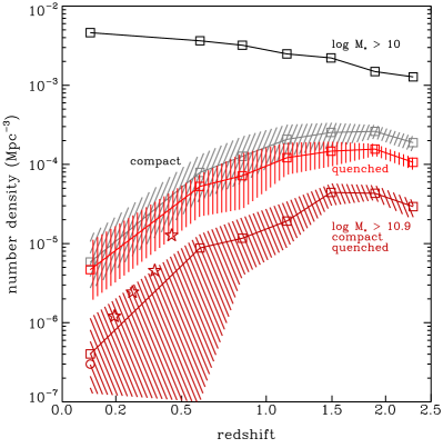
Different definitions of ultra-compact massive galaxies (UCMGs) have been used by other studies (e.g. Trujillo et al. 2009; Damjanov et al. 2014; Tortora et al. 2016; Buitrago et al. 2018). Scognamiglio et al. (2020) define UCMGs using $\log M_{*}>10.9$ ($8\times 10^{10}\mathrm{M}_{\odot}$) and $r_{50,\mathrm{circ}}<1.5\,\mathrm{kpc}$. For the UKIDSS-SDSS sample, a similar number of galaxies is obtained using $r_{50,\mathrm{maj}}<2.0\,\mathrm{kpc}$. This is shown by the grey dotted box in Fig. 10. Note that nearly all UCMGs, and all in this case, have $10.9<\log M_{*}<11.2$ (Tortora et al., 2020). From this cut, we obtained a number density of $3\times 10^{-7}\mathrm{cMpc}^{-3}$ for quenched UCMGs (15 galaxies). This is within with the upper limit at $z<0.1$ determined by Buitrago et al. (2018), and lower than the number densities of $\sim 10^{-6}\mathrm{cMpc}^{-3}$ at $z\approx 0.2$ determined by Scognamiglio et al. (2020) and of $\sim 3\times 10^{-6}\mathrm{cMpc}^{-3}$ at $0.2<z<0.6$ by Damjanov et al. (2014) (their fig. 7, UCMG lower mass limit), Our results are consistent with steep evolution in the number density at $z<0.5$ (Fig. 15).

4.6 Environment

The spectroscopic completeness of the SDSS-UKIDSS galaxy sample drops from 92% for normal-size galaxies to 76% for compact galaxies (Fig. 11). This is primarily due to fibre collisions. To evaluate the reason for and physically quantify this effect, we computed environmental densites for a selected galaxy sample.

A density-defining population (DDP) of galaxies was selected over an expanded redshift range (0.024–0.168) to avoid a redshift edge when determining densities at the sample limits of 0.04 and 0.15. The DDP was selected: (i) with $\log M_{*}>10.5$ or $\log M_{*}>10.0$ for quenched galaxies; and (ii) with a spec-z or a photo-z that had a nominal error $\zeta_{i,\mathrm{err}}^{2}<0.015$. For a calibration sample with both spec-z and good photo-z (within this error limit), 90% had $\Delta\ln(1+z)<0.015$ (difference between the spec-z and photo-z). This DDP thus supplements the spec-z with accurate photo-z enabled by the SDSS-UKIDSS data and significantly reduces biases associated with fibre collisions when measuring environmental densities.

For each galaxy, the projected distances to the three nearest DDP neighbours were determined. The neighbours had to have $\Delta v<1200$ km/s using spec-z or $\Delta v<4500$ km/s using photo-z (for either the potential neighbour and/or the target), where $\Delta v=c\Delta\ln(1+z)$ is the velocity difference (Baldry, 2018) between the target and DDP galaxy. The surface neighbour density for each galaxy is then given by

$$\log\Sigma_{{\rm ddp}}=\frac{1}{2}\log\left(\frac{2}{\pi d_{2}^{2}}\right)+\frac{1}{2}\log\left(\frac{3}{\pi d_{3}^{2}}\right)$$ (19)

where $d_{2}$ and $d_{3}$ are the projected comoving distances (cMpc) to the 2nd and 3rd nearest neighbours. This is then converted to an environmental overdensity ($\delta$) using

$$\log(1+\delta)=\log\Sigma_{{\rm ddp}}-f_{\rm ddp}(z)\mbox{~{}~{}~{},}$$ (20)

where $f_{\rm ddp}(z)$ is a fitted function for the global surface density of the DDP (in bins of 2400 km/s) that accounts for the observational flux limit because the DDP is not a volume-limited sample. For this DDP and $r_{\rm petro}<17.8$, $f_{\rm ddp}(z)$ was approximated by $f_{\rm ddp}=-0.978$ for $z\leq 0.0784$ and $-0.351-8.30\ln(1+z)$ otherwise ($-1.511$ at $z=0.15$). This ensures that the median value of $\delta$ is similar across the full redshift range for a particular type of galaxy. This was tested for both quenched and star-forming galaxies with $\log M_{*}>10.5$.

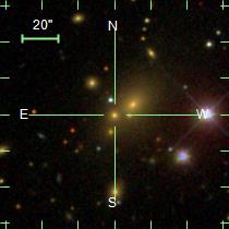
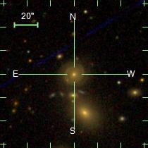
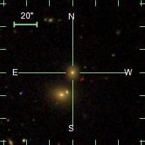
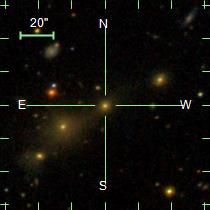
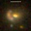
Figure 16 shows the environmental overdensity versus $\log\Sigma_{1.5}$ for the quenched galaxies. The lower panel shows the fraction of galaxies in high density environments with $\log(1+\delta)>1.5$. From this, there is a clear difference with $69\pm 8$% of the most compact galaxies ($>10.6$) found in high density environments compared to 24% for normal-size quenched galaxies. This noticeable effect is in contrast to the median $\log\Sigma_{1.5}$ that is 9.875 in high-density environments compared to 9.866 at lower densities. In other words, for quenched galaxies, there are small or negligible differences between the general size-mass relations at low redshift (Maltby et al., 2010; Matharu et al., 2019). Matharu et al. noted that while minor mergers in clusters are less likely than in the field, the dissapearance of compact cluster galaxies that are seen at high redshift can be explained by a combination of mergers with the brightest cluster galaxy and being tidally destroyed. For the rarer compact galaxies, they are nevertheless more likely to survive in high-density environments (Poggianti et al., 2013; Trujillo et al., 2014; Buitrago et al., 2018). This is demonstrated conclusively using this complete SDSS-UKIDSS sample (see Fig. 20 for images of compact galaxies in high-density environments).

Figure 16: Upper panel: environmental densities for the quenched galaxy sample ($0.04<z<0.15$). Lower panel: fraction of galaxies in high density environments. The circles represent galaxies with $\log\Sigma_{1.5}>10.5$ (black with spec-z and orange with photo-z)

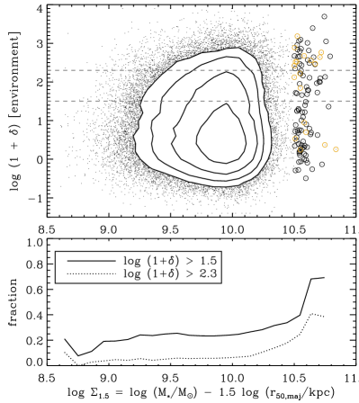
This result is consistent with analysis of Peralta de Arriba et al. (2016), using an SDSS sample, who showed that the fraction of relics (compact early types) relative to normal-sized early types was higher in high-density environments. For our sample, we find that 0.7% of quenched massive galaxies are compact ($\log\Sigma_{1.5}>10.5$) in high density environments ($\log(1+\delta)>2.3$) compared to 0.1% in low density ($\log(1+\delta)<1.5$). For $\log\Sigma_{1.5}>10.2$, we find 7.8% compared to 3.7%. Damjanov et al. (2015) found a neglible difference between the environments of compact and non-compact quiescent galaxies when controlling for stellar mass (their fig. 10) at $0.1<z<0.4$. Tortora et al. (2020) found UCMGs to be slightly more abundant in clusters compared to the field when restricting the comparison sample to $10.9<\log M_{*}<11.2$ at $z\sim 0.4$ (their fig. 1). These differences compared to the SDSS-UKIDSS sample could arise from the types of density measurements, the mass range or from evolution since $z\sim 0.4$.

5 Summary

The primary aim of this analysis was to determine the number density of compact galaxies using a complete sample with photometry from SDSS and UKIDSS. After masking around GAIA stars (Figs. 1–2), rather than using a not-saturated criterion, and selecting galaxies using primarily colours ($JKgi$, $YKgz$, Figs. 3–4), a sample of 245 645 sources was obtained covering $2300\,{\rm deg}^{2}$ to $r<17.8$. The majority (92%) of the sample were selected without using a profile separator, i.e. with no bias against compact galaxies, with the additional selection being mainly extended sources that did not have catalog-matched UKIDSS photometry and which were added in for completeness.

To refine the sample further, photo-z were determined using an accurate scaled flux matching (SFM) empirical method. The matching set were galaxies with reliable spec-z and photometry. A photo-z estimate can be obtained for any source even if it is missing or has bad photometry in one or more bands. The criteria for a reliable photo-z estimate were determined using: the number of matches within a chi-squared limit (Fig. 5), and the estimate of the error (Fig. 6). For sources with reliable spec-z and photo-z, the 68th percentile of $|\Delta\ln(1+z)|$ was 0.0125 (0.010 for quenched galaxies, 0.016 for star-forming galaxies) and 99.7% were within 0.06 (Fig. 7). These photo-z were more accurate than the SDSS Beck et al. (2016) photo-z because of the additional near-IR photometry.

Sources were assigned reliable photo-z if reliable spec-z were not available; otherwise they were not included and assumed to be stars or quasars. The selection of sources with $0.04<z<0.15$ produced a sample of 163 186 galaxies (10.4% with photo-z, Fig. 8). Utilizing SDSS pipeline half-light radii that were shown to be similar to the sizes from the two-component fits of Simard et al. (2011) (Fig. 9), a size-mass distribution was produced (Fig. 10). This is complete for compact galaxies because of the colour selection and photo-z. The slope of the high-mass relation for quiescent galaxies is is about 2/3, and thus following Barro et al. (2013), we computed $\Sigma_{1.5}$ ($M_{*}/r_{50,\mathrm{maj}}^{1.5}$ in $\mathrm{M}_{\odot}\mathrm{kpc}^{-1.5}$, Eq. 4.3) that runs perpendicular to this slope. The spectroscopic completeness drops from 92% for normal-size galaxies to 76% for compact galaxies with $\log\Sigma_{1.5}>10.5$ (Fig. 11) ($\log M_{*}>10$). This can be attributed primarily to fibre collisions, and thus environments, rather than incompleteness of the SDSS target selection.

A high-z comparison sample was obtained from 3D-HST data with structural measurements from van der Wel et al. (2012) and stellar masses from Driver et al. (2018). The evolution in the $\log\Sigma_{1.5}$ distribution functions (Fig.13) from high to low redshift shows: a gradual rise in the number density at $\log\Sigma_{1.5}\la 10$; while at $>10$, there is a sharp cutoff in the number density at lower redshifts. In the SDSS-UKIDSS sample, the number densities of compact galaxies are about a factor of 30–100 below the peak at $z\sim 2$ (Fig. 15). The consensus mechanism for the growth of compact galaxies is primarily via minor mergers.

Comparing the distribution functions with different redshift snapshots from the EAGLE hydrodynamical simulation shows good qualitative agreement (Fig. 14). In addition to the GSMF (Fig. 12) and size-mass relations, using $\log\Sigma_{1.5}$ distributions is an informative way to compare simulations with data because the number densities for both normal-size and compact galaxies are clearly conveyed. This is an avenue for future research, for example, for simulations that agree with observations, the past merger history and environments of quenched galaxies with different low- and high-redshift $\log\Sigma_{1.5}$ values could be compared.

We searched amongst the entire population of (more than two million) stars and galaxies to $r<17.8$, using 9-band photometry, for compact galaxies. This confirmed the low number densities ($\la 10^{-5}\,\mathrm{cMpc}^{-3}$) of local compact galaxies in agreement with the SDSS analysis of Taylor et al. (2010). The $\log\Sigma_{1.5}$ distribution of local quenched galaxies is similar in low- and high-density environments (Fig. 16 upper panel). However, the rare compact galaxies are significantly more likely to survive in high density environments (Fig. 16 lower panel).

There is substantial evolution in the size-mass distribution since $z\sim 1$. In the future, the WAVES-DEEP survey with 4MOST aims to obtain redshifts for galaxies to $z\la 0.8$ over $\sim 60\,{\rm deg}^{2}$ (Driver et al., 2019). Coupled with Euclid imaging (Laureijs et al., 2010; da Silva et al., 2019), this will provide galaxy structural measurements over a cosmic volume that is sufficient to divide the sample into several epochs and different types of environments. The diversification of the compact galaxy population will be illuminated in detail.

Data Availability

The data underlying this article were accessed from: the Sloan Digital Sky Survey at skyserver.sdss.org/ (dr14.PhotoPrimary, dr14.SpecObj, dr14.Photoz, dr7.PhotoObjAll); the WFCAM Science Archive at wsa.roe.ac.uk/ for the UKIDSS data (lasYJHKsource); the Gaia archive at gea.esac.esa.int/archive/ (gaiadr2.gaia_source); and the 3D-HST archive at 3dhst.research.yale.edu/ [the catalog is also available via ADS 2015yCat..22140024S (Skelton et al., 2014)]. Galaxy structural measurements can be accessed via ADS 2011yCat..21960011S (Simard et al., 2011) and ADS 2012yCat..22030024V (van der Wel et al., 2012).

The derived data generated in this research will be shared at www.astro.ljmu.ac.uk/~ikb/research/ or on reasonable request to the corresponding author.

Appendix A Size tests and Images

This paper uses the SDSS pipeline profile fits for the estimates of the half-light radii (§ 4.2). The photometric pipeline was constructed by Lupton et al. (2001) and is described primarily in § 4.4 of Stoughton et al. (2002) with updates in other data release papers (e.g. Abazajian et al. 2004). The measurements are robust because the de Vaucouleurs (Sersic $n=4$) and exponential (Sersic $n=1$) profiles are fitted separately. Therefore, minimization problems are less severe compared to simultaneous bulge-plus-disk fitting or allowing for a free Sersic index (e.g. Simard et al. 2011; Kelvin et al. 2012). In addition, the local PSF is well determined and accounts for the variation across each detector chip (§ 4.3 of Stoughton et al.). This variation is only 1-dimensional because SDSS images were obtained using drift scanning. This is a notable advantage for empirical PSF determination compared to typical point-and-stare integrations.

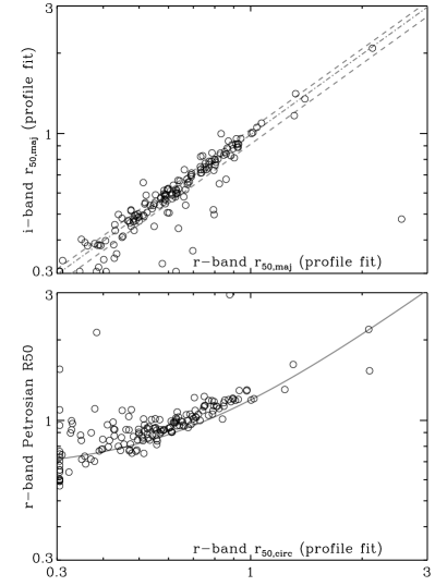
For the half-light radii, we used a weighted average of the profile radii for each galaxy (Eq. 16). Figure 17 (top) shows a comparison between $r$- and $i$-band $r_{50,\mathrm{maj}}$ measurements for compact galaxies. For these galaxies, the median ratio is 0.99 ($i$- divide $r$-band size) and there is good agreement between the measurements with 93% differing by less than 0.1 dex. An alternative measure of half-light radius obtained by the SDSS pipeline is using the Petrosian magnitude with circular apertures (petroR50, Stoughton et al. 2002). Figure 17 (bottom) shows petroR50 versus the circularized half-light radii from the profile fits. The petroR50 measurement includes the effects of the PSF. To account for this, the solid shows a simple correction with 0.65 added in quadrature to x-axis value, where $0.65^{\prime\prime}$ is median value of petroR50 for stars in the SDSS-UKIDSS sample. While most of the petroR50 values lie above this line, 90% are within 0.1 dex. The profile-fit radii will be more accurate as they account for the variable PSF. There is sufficient agreement to demonstrate the internal consistency of the SDSS half-light radii.

Figure 17: Internal size tests for the compact galaxies with $\log\Sigma_{1.5}>10.5$. Top panel: comparison between $r$- and $i$-band measurements from the profile fits (units of arcsec). The dot-dash line shows the median ratio, while the dashed lines show the 16th and 84th percentiles. Bottom panel: comparison between the Petrosian half-light radii and the profile fits. The solid line shows $y=\sqrt{(}x^{2}+0.65^{2})$ as a simple guide to account approximately for the effect of the PSF on the petroR50 sizes.

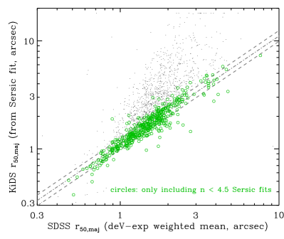
To compare with an external dataset, we used the $r$-band structural parameters determined by Roy et al. (2018), and presented in Tortora et al. (2018), based on the imaging from the Kilo Degree Survey (KiDS, de Jong et al. 2017). The mean PSF full width half maximum (FWHM) is $0.7^{\prime\prime}$ and thus higher resolution than the SDSS which has a median of $1.3^{\prime\prime}$. The comparison set of galaxies was expanded to $\log\Sigma_{1.5}>10$ (using the smaller $r_{50,\mathrm{maj}}$ from KiDS or SDSS) and $0.04<z<0.2$ because the overlap area was only about $200\,{\rm deg}^{2}$ to give a sample of 1674 galaxies. Figure 18 shows the comparison between the half-light radii determined from KiDS (that used a Sersic fit) with SDSS. Notably, there are many outliers shown by the points, however, these occur primarily when the Sersic index $n$ is above 4.5. A unrealistic fraction of galaxies (72%) are fitted with $n>4.5$ in the KiDS process. Restricting the sample to only those galaxies where the KiDS process fitted the galaxies with $n<4.5$ (469 galaxies), shown by the green circles, results in good agreement between the KiDS and SDSS sizes. For these, the median offset of the KiDS sizes is $+0.04$ dex and 84% differ by less than 0.1 dex. We conclude that the SDSS sizes are more robust that the sizes determined from KiDS with a free Sersic index, with sufficient agreement with $n<4.5$ to demonstrate that the SDSS sizes are not substantially underestimating the half-light radii.

Figure 18: Comparison between half-light radii from KiDS with SDSS. The dot-dash line shows the median ratio, while the dashed lines show the 16th and 84th percentiles for the sample shown by green circles.

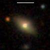
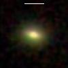
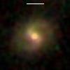
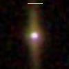
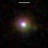
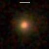
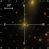
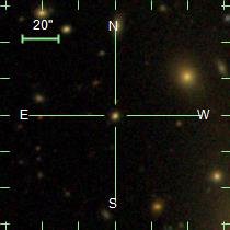
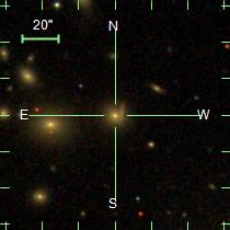
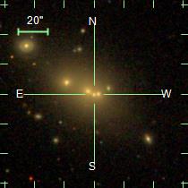
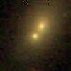
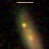
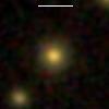
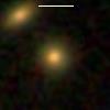
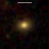
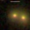
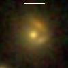
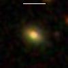
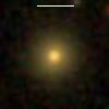
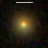
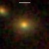
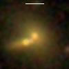
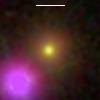
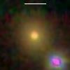
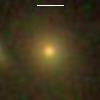
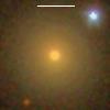
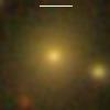
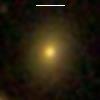
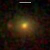
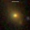
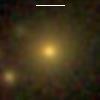
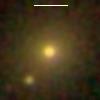
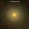
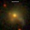
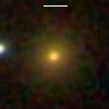
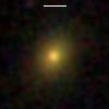
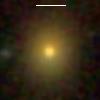
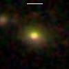
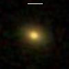
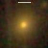
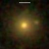
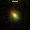
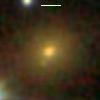
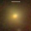
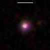
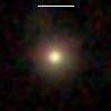
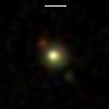
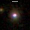
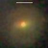
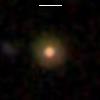
The final check on the compact galaxies is visual inspection, noting that those in areas of severe scattered light, not accounted for by the GAIA masking, have been rejected from the sample. Images were obtained from the SDSS cutout service (Nieto-Santisteban et al., 2004) scaled as per Lupton et al. (2004). Figure 19 shows a selection of 48 out of the 164 compact galaxies. Each image clearly shows a concentration of light within a small area ($\sim 2^{\prime\prime}$) with the size of the core being determined by the PSF in many cases. By chance, the first image in row six shows a possible lense of a background galaxy (coordinates 343.09313, $+01.11666$; Diehl et al. 2017).

Note that a number of images show an obvious extended halo around the compact core. The use of the arcsinh stretch (Lupton et al., 2004) is specifically designed to highlight low-surface-brightness features at the same time as preserving the structure of bright sources. Nevertheless, an extended halo may indicate that the SDSS pipeline half-light radii apply to the core and not to the whole galaxy. Taking a sample of 111 compact galaxies that are quenched ($\log\Sigma_{1.5}>10.5$ and $r_{50,\mathrm{maj}}<2$), we tested this by using the PhotoProfile measurements from SDSS to determine $r$-band aperture magnitudes out to radii of 5 kpc and 20 kpc (total flux for this test) where available. From these and by visual inspection (to rule out problems with the aperture magnitudes), only about 15 out of 111 have $>10$% of their total flux at radii larger than 5 kpc, with the median being 3%. For 40 star-forming compact galaxies, the median is 13% of the total flux at $r>5\,\mathrm{kpc}$ in the $r$-band. For all 164 galaxies with $\log\Sigma_{1.5}>10.5$, these total aperture magnitudes differ from the cmodel magnitudes by less than 0.10 mag for 150 galaxies, and by less than 0.15 mag for 159 galaxies. This demonstrates that the SDSS pipeline profile fits are accounting for most of the flux, and are thus sufficiently representative of each galaxy for determining the half-light radii and masses.

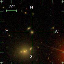
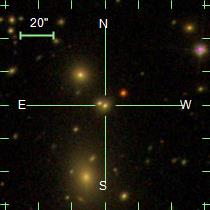
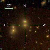
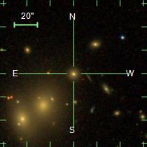
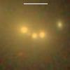
Figure 20 shows a larger sky area around a sample of the compact galaxies in high-density regions. These images demonstrate the fidelity of the compact galaxy sample.

10.0
10.4
10.6
10.7
10.8
11.0
10.3
10.6

Figure 19: Images of compact galaxies ($\log\Sigma_{1.5}>10.5$). Most images are $20^{\prime\prime}\times 20^{\prime\prime}$; ten images centred on galaxies at $z<0.08$ were scaled to $30\times 30\,\mathrm{kpc}$. The white bar at the top of each image represents 10 kpc at the redshift of the central galaxy. The top six rows show the quenched the population, while the remaining two rows show galaxies with higher star-formation rates. The images are ordered from the lowest to highest in stellar mass (10.0–11.4) within each subsample, and are evenly selected by mass from the 164 shown with circles in Fig. 10. The mass ($\log M_{*}$) is noted for the first image in each row. The arcsinh stretch used to produce the images ($i$-$r$-$g\rightarrow$RGB) is described by Lupton et al. (2004).

Figure 20: Images centred on compact galaxies in high-density environments. The second image has two compact galaxies. The images are selected from the compact galaxies with $\log(1+\delta)>2.3$ shown in Fig. 16.

References

- Abazajian et al. (2004) Abazajian K., et al., 2004, AJ, 128, 502
- Babbedge et al. (2004) Babbedge T. S. R. et al., 2004, MNRAS, 353, 654
- Baldry (2018) Baldry I. K., 2018, arXiv:1812.05135
- Baldry et al. (2006) Baldry I. K., Balogh M. L., Bower R. G., Glazebrook K., Nichol R. C., Bamford S. P., Budavari T., 2006, MNRAS, 373, 469
- Baldry et al. (2018) Baldry I. K. et al., 2018, MNRAS, 474, 3875
- Baldry et al. (2010) Baldry I. K. et al., 2010, MNRAS, 404, 86
- Barro et al. (2013) Barro G. et al., 2013, ApJ, 765, 104
- Barro et al. (2014) Barro G. et al., 2014, ApJ, 791, 52
- Beck et al. (2016) Beck R., Dobos L., Budavári T., Szalay A. S., Csabai I., 2016, MNRAS, 460, 1371
- Bezanson et al. (2009) Bezanson R., van Dokkum P. G., Tal T., Marchesini D., Kriek M., Franx M., Coppi P., 2009, ApJ, 697, 1290
- Blanton et al. (2005) Blanton M. R., et al., 2005, AJ, 129, 2562
- Boylan-Kolchin et al. (2006) Boylan-Kolchin M., Ma C.-P., Quataert E., 2006, MNRAS, 369, 1081
- Brammer et al. (2008) Brammer G. B., van Dokkum P. G., Coppi P., 2008, ApJ, 686, 1503
- Brammer et al. (2012) Brammer G. B. et al., 2012, ApJS, 200, 13
- Brinchmann et al. (2004) Brinchmann J., Charlot S., White S., Tremonti C., Kauffmann G., Heckman T., Brinkmann J., 2004, MNRAS, 351, 1151
- Bryant et al. (2015) Bryant J. J. et al., 2015, MNRAS, 447, 2857
- Buitrago et al. (2018) Buitrago F. et al., 2018, A&A, 619, A137
- Buitrago et al. (2008) Buitrago F., Trujillo I., Conselice C. J., Bouwens R. J., Dickinson M., Yan H., 2008, ApJ, 687, L61
- Buitrago et al. (2017) Buitrago F., Trujillo I., Curtis-Lake E., Montes M., Cooper A. P., Bruce V. A., Pérez-González P. G., Cirasuolo M., 2017, MNRAS, 466, 4888
- Cappellari et al. (2012) Cappellari M. et al., 2012, Nature, 484, 485
- Carollo et al. (2013) Carollo C. M. et al., 2013, ApJ, 773, 112
- Cassata et al. (2013) Cassata P. et al., 2013, ApJ, 775, 106
- Chabrier (2003) Chabrier G., 2003, PASP, 115, 763
- Charbonnier et al. (2017) Charbonnier A. et al., 2017, MNRAS, 469, 4523
- Cimatti et al. (2004) Cimatti A. et al., 2004, Nature, 430, 184
- Collier et al. (2018) Collier W. P., Smith R. J., Lucey J. R., 2018, MNRAS, 478, 1595
- Connolly et al. (1995) Connolly A. J., Csabai I., Szalay A. S., Koo D. C., Kron R. G., Munn J. A., 1995, AJ, 110, 2655
- Conroy & van Dokkum (2012) Conroy C., van Dokkum P. G., 2012, ApJ, 760, 71
- Crain et al. (2015) Crain R. A. et al., 2015, MNRAS, 450, 1937
- da Cunha et al. (2008) da Cunha E., Charlot S., Elbaz D., 2008, MNRAS, 388, 1595
- da Silva et al. (2019) da Silva R. et al., 2019, in ASP Conf. Ser., Vol. 521, ADASS XXVI, Molinaro M., Shortridge K., Pasian F., eds., p. 311
- Daddi et al. (2005) Daddi E. et al., 2005, ApJ, 626, 680
- Damjanov et al. (2014) Damjanov I., Hwang H. S., Geller M. J., Chilingarian I., 2014, ApJ, 793, 39
- Damjanov et al. (2009) Damjanov I. et al., 2009, ApJ, 695, 101
- Damjanov et al. (2015) Damjanov I., Zahid H. J., Geller M. J., Hwang H. S., 2015, ApJ, 815, 104
- Davidzon et al. (2013) Davidzon I. et al., 2013, A&A, 558, A23
- de Jong et al. (2017) de Jong J. T. A. et al., 2017, A&A, 604, A134
- de la Rosa et al. (2016) de la Rosa I. G., La Barbera F., Ferreras I., Sánchez Almeida J., Dalla Vecchia C., Martínez-Valpuesta I., Stringer M., 2016, MNRAS, 457, 1916
- Deeley et al. (2020) Deeley S. et al., 2020, arXiv e-prints, arXiv:2008.02426
- Devour & Bell (2017) Devour B. M., Bell E. F., 2017, MNRAS, 468, L31
- Diehl et al. (2017) Diehl H. T. et al., 2017, ApJS, 232, 15
- Driver et al. (2018) Driver S. P. et al., 2018, MNRAS, 475, 2891
- Driver et al. (2019) Driver S. P. et al., 2019, The Messenger, 175, 46
- Driver et al. (2016) Driver S. P. et al., 2016, MNRAS, 455, 3911
- Dye et al. (2006) Dye S., et al., 2006, MNRAS, 372, 1227
- Eales (1993) Eales S., 1993, ApJ, 404, 51
- Fan et al. (2010) Fan L., Lapi A., Bressan A., Bernardi M., De Zotti G., Danese L., 2010, ApJ, 718, 1460
- Fan et al. (2008) Fan L., Lapi A., De Zotti G., Danese L., 2008, ApJ, 689, L101
- Ferré-Mateu et al. (2017) Ferré-Mateu A., Trujillo I., Martín-Navarro I., Vazdekis A., Mezcua M., Balcells M., Domínguez L., 2017, MNRAS, 467, 1929
- Firth et al. (2003) Firth A. E., Lahav O., Somerville R. S., 2003, MNRAS, 339, 1195
- Furlong et al. (2017) Furlong M. et al., 2017, MNRAS, 465, 722
- Gaia Collaboration et al. (2016) Gaia Collaboration et al., 2016, A&A, 595, A1
- Gao & Fan (2020) Gao Y., Fan L.-L., 2020, Research in Astronomy and Astrophysics, 20, 106
- Gargiulo et al. (2016) Gargiulo A., Saracco P., Tamburri S., Lonoce I., Ciocca F., 2016, A&A, 592, A132
- Graham et al. (2015) Graham A. W., Dullo B. T., Savorgnan G. A. D., 2015, ApJ, 804, 32
- Grogin et al. (2011) Grogin N. A. et al., 2011, ApJS, 197, 35
- Gu et al. (2020) Gu Y., Fang G., Yuan Q., Lu S., 2020, PASP, 132, 054101
- Hill et al. (2011) Hill D. T., et al., 2011, MNRAS, 412, 765
- Hilz et al. (2012) Hilz M., Naab T., Ostriker J. P., Thomas J., Burkert A., Jesseit R., 2012, MNRAS, 425, 3119
- Hopkins et al. (2010) Hopkins P. F. et al., 2010, ApJ, 715, 202
- Huang et al. (2013) Huang S., Ho L. C., Peng C. Y., Li Z.-Y., Barth A. J., 2013, ApJ, 768, L28
- Huchra et al. (2012) Huchra J. P. et al., 2012, ApJS, 199, 26
- Huertas-Company et al. (2016) Huertas-Company M. et al., 2016, MNRAS, 462, 4495
- Kawinwanichakij et al. (2020) Kawinwanichakij L. et al., 2020, ApJ, 892, 7
- Kelvin et al. (2012) Kelvin L. S. et al., 2012, MNRAS, 421, 1007
- Koo (1999) Koo D. C., 1999, in ASP Conf. Ser., Vol. 191, Photometric Redshifts and the Detection of High Redshift Galaxies, Weymann R., Storrie-Lombardi L., Sawicki M., Brunner R., eds., p. 3
- Kriek et al. (2006) Kriek M. et al., 2006, ApJ, 649, L71
- Kroupa (2001) Kroupa P., 2001, MNRAS, 322, 231
- La Barbera et al. (2013) La Barbera F., Ferreras I., Vazdekis A., de la Rosa I. G., de Carvalho R. R., Trevisan M., Falcón-Barroso J., Ricciardelli E., 2013, MNRAS, 433, 3017
- Lange et al. (2015) Lange R. et al., 2015, MNRAS, 447, 2603
- Laureijs et al. (2010) Laureijs R. J., Duvet L., Escudero Sanz I., Gondoin P., Lumb D. H., Oosterbroek T., Saavedra Criado G., 2010, Proc. SPIE, 7731, 77311H
- Lawrence et al. (2007) Lawrence A., et al., 2007, MNRAS, 379, 1599
- Liske et al. (2006) Liske J., Driver S. P., Allen P. D., Cross N. J. G., De Propris R., 2006, MNRAS, 369, 1547
- Longhetti et al. (2007) Longhetti M. et al., 2007, MNRAS, 374, 614
- Lu et al. (2019) Lu S.-Y., Gu Y.-Z., Fang G.-W., Yuan Q.-R., 2019, Research in Astronomy and Astrophysics, 19, 150
- Lupton et al. (2004) Lupton R., Blanton M. R., Fekete G., Hogg D. W., O’Mullane W., Szalay A., Wherry N., 2004, PASP, 116, 133
- Lupton et al. (2001) Lupton R. H., Gunn J. E., Ivezić Z., Knapp G. R., Kent S., Yasuda N., 2001, in ASP Conf. Ser., Vol. 238, ADASS X, Harnden F. R., et al., eds., ASP, San Francisco, p. 269
- Lupton et al. (1999) Lupton R. H., Gunn J. E., Szalay A. S., 1999, AJ, 118, 1406
- Maltby et al. (2010) Maltby D. T. et al., 2010, MNRAS, 402, 282
- Martín-Navarro et al. (2019) Martín-Navarro I., van de Ven G., Yıldırım A., 2019, MNRAS, 487, 4939
- Matharu et al. (2019) Matharu J. et al., 2019, MNRAS, 484, 595
- McAlpine et al. (2016) McAlpine S. et al., 2016, Astronomy and Computing, 15, 72
- Momcheva et al. (2016) Momcheva I. G. et al., 2016, ApJS, 225, 27
- Mortlock et al. (2015) Mortlock A. et al., 2015, MNRAS, 447, 2
- Muzzin et al. (2013) Muzzin A. et al., 2013, ApJ, 777, 18
- Naab et al. (2009) Naab T., Johansson P. H., Ostriker J. P., 2009, ApJ, 699, L178
- Nieto-Santisteban et al. (2004) Nieto-Santisteban M. A., Szalay A. S., Gray J., 2004, in ASP Conf. Ser., Vol. 314, ADASS XIII, Ochsenbein F., Allen M. G., Egret D., eds., p. 666
- Noeske et al. (2007) Noeske K. G. et al., 2007, ApJ, 660, L47
- Pearson et al. (2018) Pearson W. J. et al., 2018, A&A, 615, A146
- Peralta de Arriba et al. (2016) Peralta de Arriba L., Quilis V., Trujillo I., Cebrián M., Balcells M., 2016, MNRAS, 461, 156
- Poggianti et al. (2013) Poggianti B. M. et al., 2013, ApJ, 762, 77
- Popesso et al. (2019) Popesso P. et al., 2019, MNRAS, 490, 5285
- Posacki et al. (2015) Posacki S., Cappellari M., Treu T., Pellegrini S., Ciotti L., 2015, MNRAS, 446, 493
- Quilis & Trujillo (2013) Quilis V., Trujillo I., 2013, ApJ, 773, L8
- Ragone-Figueroa & Granato (2011) Ragone-Figueroa C., Granato G. L., 2011, MNRAS, 414, 3690
- Roy et al. (2018) Roy N. et al., 2018, MNRAS, 480, 1057
- Salim et al. (2007) Salim S. et al., 2007, ApJS, 173, 267
- Saulder et al. (2015) Saulder C., van den Bosch R., Mieske S., 2015, A&A, 578, A134
- Schaye et al. (2015) Schaye J. et al., 2015, MNRAS, 446, 521
- Scognamiglio et al. (2020) Scognamiglio D. et al., 2020, ApJ, 893, 4
- Sedgwick et al. (2019a) Sedgwick T. M., Baldry I. K., James P. A., Kelvin L. S., 2019a, MNRAS, 484, 5278
- Sedgwick et al. (2019b) Sedgwick T. M., Baldry I. K., James P. A., Kelvin L. S., 2019b, arXiv:1909.04535
- Shen et al. (2003) Shen S., Mo H. J., White S. D. M., Blanton M. R., Kauffmann G., Voges W., Brinkmann J., Csabai I., 2003, MNRAS, 343, 978
- Simard et al. (2011) Simard L., Mendel J. T., Patton D. R., Ellison S. L., McConnachie A. W., 2011, ApJS, 196, 11
- Simard et al. (2002) Simard L., et al., 2002, ApJS, 142, 1
- Skelton et al. (2014) Skelton R. E. et al., 2014, ApJS, 214, 24
- Smith & Lucey (2013) Smith R. J., Lucey J. R., 2013, MNRAS, 434, 1964
- Sonnenfeld et al. (2014) Sonnenfeld A., Nipoti C., Treu T., 2014, ApJ, 786, 89
- Stoughton et al. (2002) Stoughton C., et al., 2002, AJ, 123, 485
- Strauss et al. (2002) Strauss M. A., et al., 2002, AJ, 124, 1810
- Suess et al. (2019) Suess K. A., Kriek M., Price S. H., Barro G., 2019, ApJ, 877, 103
- Szomoru et al. (2012) Szomoru D., Franx M., van Dokkum P. G., 2012, ApJ, 749, 121
- Taylor et al. (2010) Taylor E. N., Franx M., Glazebrook K., Brinchmann J., van der Wel A., van Dokkum P. G., 2010, ApJ, 720, 723
- Tortora et al. (2016) Tortora C. et al., 2016, MNRAS, 457, 2845
- Tortora et al. (2020) Tortora C. et al., 2020, A&A, 638, L11
- Tortora et al. (2018) Tortora C. et al., 2018, MNRAS, 481, 4728
- Trujillo et al. (2009) Trujillo I., Cenarro A. J., de Lorenzo-Cáceres A., Vazdekis A., de la Rosa I. G., Cava A., 2009, ApJ, 692, L118
- Trujillo et al. (2007) Trujillo I., Conselice C. J., Bundy K., Cooper M. C., Eisenhardt P., Ellis R. S., 2007, MNRAS, 382, 109
- Trujillo et al. (2014) Trujillo I., Ferré-Mateu A., Balcells M., Vazdekis A., Sánchez-Blázquez P., 2014, ApJ, 780, L20
- Valentinuzzi et al. (2010) Valentinuzzi T. et al., 2010, ApJ, 712, 226
- van der Wel et al. (2012) van der Wel A. et al., 2012, ApJS, 203, 24
- van der Wel et al. (2014) van der Wel A. et al., 2014, ApJ, 788, 28
- van Dokkum et al. (2014) van Dokkum P. G. et al., 2014, ApJ, 791, 45
- van Dokkum et al. (2008) van Dokkum P. G. et al., 2008, ApJ, 677, L5
- van Dokkum et al. (2015) van Dokkum P. G. et al., 2015, ApJ, 813, 23
- Wellons et al. (2015) Wellons S. et al., 2015, MNRAS, 449, 361
- Wolf (2009) Wolf C., 2009, MNRAS, 397, 520
- Wright et al. (2018) Wright A. H., Driver S. P., Robotham A. S. G., 2018, MNRAS, 480, 3491
- Yıldırım et al. (2017) Yıldırım A., van den Bosch R. C. E., van de Ven G., Martín-Navarro I., Walsh J. L., Husemann B., Gültekin K., Gebhardt K., 2017, MNRAS, 468, 4216
- York et al. (2000) York D. G., et al., 2000, AJ, 120, 1579