Pseudo-Goldstone dark matter: gravitational waves and direct-detection blind spots

Abstract

Pseudo-Goldstone dark matter is a thermal relic with momentum-suppressed direct-detection cross section. We study the most general model of pseudo-Goldstone dark matter arising from the complex-singlet extension of the Standard Model. The new U(1) symmetry of the model is explicitly broken down to a CP-like symmetry stabilising dark matter. We study the interplay of direct-detection constraints with the strength of cosmic phase transitions and possible gravitational-wave signals. While large U(1)-breaking interactions can generate a large direct-detection cross section, there are blind spots where the cross section is suppressed. We find that sizeable cubic couplings can give rise to a first-order phase transition in the early universe. We show that there exist regions of the parameter space where the resulting gravitational-wave signal can be detected in future by the proposed Big Bang Observer detector.

1 Introduction

Recent direct-detection results have imposed severe constraints Akerib:2016vxi ; Aprile:2018dbl ; Cui:2017nnn on some of the most popular dark matter (DM) frameworks, such as the real-scalar-singlet extension of the Standard Model (SM). Pseudo-Goldstone DM is a simple framework with a naturally small direct-detection cross section due to suppressed scattering rates at low momentum transfer resulting from the derivative interactions of the Goldstone boson.

In the minimal pseudo-Goldstone DM model Gross:2017dan ; Huitu:2018gbc ; Alanne:2018zjm ; Azevedo:2018oxv ; Karamitros:2019ewv ; Cline:2019okt ; Arina:2019tib (see also refs. Barger:2008jx ; Chiang:2017nmu ), the global U(1) symmetry is explicitly broken down to a $\mathbb{Z}_{2}$ symmetry by the DM mass term. In this case, the electroweak phase transition is of second order Kannike:2019wsn . If the U(1) symmetry is explicitly broken to $\mathbb{Z}_{3}$ Kannike:2019mzk or to nothing, the resulting cubic terms of the general model can induce, in part of the parameter space, strong first-order phase transitions Witten:1984rs ; Hogan:1984hx ; Steinhardt:1981ct leading to a gravitational-wave (GW) signal detectable by LISA Audley:2017drz ; Baker:2019nia , DECIGO Seto:2001qf ; Kawamura:2006up ; Yagi:2011wg ; Isoyama:2018rjb , or BBO Crowder:2005nr ; Corbin:2005ny ; Harry:2006fi . These cubic couplings have also been considered in a different context, e.g., in refs. Jiang:2015cwa ; Alves:2018oct ; Alves:2018jsw .

The tree-level direct-detection cross section vanishes — in the limit of zero momentum transfer — only in the case of the $\mathbb{Z}_{2}$- symmetric pseudo-Goldstone DM model with the U(1) symmetry softly broken by a mass term Gross:2017dan . In general, interaction terms that explicitly break the U(1) also yield contributions to the direct-detection cross section at tree level which do not vanish at zero momentum transfer. At one-loop level the zero-momentum-transfer cross section is non-vanishing already in the $\mathbb{Z}_{2}$-symmetric model Alanne:2018zjm ; Azevedo:2018exj ; Ishiwata:2018sdi .

These features can be understood as follows. The vanishing of the cross section at zero momentum transfer is a manifestation of the underlying continuous global symmetry; in the absence of any explicit symmetry-breaking terms, the prospective DM candidate is an exact Goldstone boson and therefore has only derivative interactions, which yield zero cross section in the $t\to 0$ limit in elastic scattering processes. An exact Goldstone boson would of course be massless, which is why the minimal model must contain at least the $\mathbb{Z}_{2}$-symmetric mass term which breaks U(1), but yields a vanishing zero-momentum-transfer cross section at tree level. Any other operator breaking the symmetry explicitly, and thereby contributing to the mass of the pseudo-Goldstone boson, results in a non-vanishing zero-momentum-transfer cross section already at tree level.

Our aim is to study the most general model of pseudo-Goldstone DM arising from the complex-singlet extension of the SM; the parameter space studied here has some overlap with that of ref. Chao:2017vrq . The scalar potential in this model is inevitably CP-conserving Branco:1999fs , and the only symmetry of the potential is the CP-like $S\to S^{*}$ invariance which stabilises the imaginary part of the complex singlet, $S$. In particular, we seek to study the correlation between the direct-detection cross section and the strength of the electroweak phase transition. We take into account theoretical constraints from perturbativity, unitarity and vacuum stability together with experimental constraints on the invisible width of the Higgs boson and on the Higgs-singlet mixing angle.

Our main result relevant for direct detection of pseudo-Goldstone DM is that in this model certain combinations of parameters appear in both the pseudo-Goldstone mass and the $t\to 0$ cross section. Setting such a combination to zero then makes the direct-detection cross section vanish at tree level (but not at loop level) on a slice of the parameter space. On the other hand, we will uncover regions of parameter space where the model has sufficiently strong first-order finite-temperature phase transition so that the associated gravitational-wave signal can be detected in future satellite observatories. There is a significant correlation between the strength of the gravitational-wave signal and direct-detection cross section: Increasing the former will also make the pseudo-Goldstone DM more easily detectable, while suppressing the latter typically results in a weak phase transition.

The paper is organised as follows: We introduce the general complex-singlet model in section 2. In section 3 we discuss DM phenomenology including direct and indirect detection. Cosmic phase transitions are considered in section 4, and we conclude in section 5. The appendices contain some more technical details: In appendix A we give the formulae for shifting away the linear term in the potential, appendix B lists the annihilation cross sections, appendix C shows how the one-loop contribution to the direct-detection cross section is modified in the presence of cubic symmetry-breaking terms, and in appendix D we list the one-loop renormalisation group equations for the model.

2 General complex-singlet model

We consider a model where the scalar sector consists of the SM Higgs doublet, $H$, and a complex singlet, $S$. The model is by construction CP-conserving Branco:1999fs , i.e. invariant under the CP-like transformation $S\rightarrow S^{\ast}$. We write the potential as

$$V_{\rm tree}=V_{0}+V_{\rm br},$$ (1)

where

$$V_{0}=\mu_{H}^{2}H^{\dagger}H+\mu_{S}^{2}S^{*}S+\lambda_{H}(H^{\dagger}H)^{2}+\lambda_{HS}(H^{\dagger}H)S^{*}S+\lambda_{S}(S^{*}S)^{2}$$ (2)

is invariant under a global U(1) transformation $S\to e^{i\phi}S$, while the remaining part explicitly breaks the U(1) symmetry:

$$\begin{split}V_{\rm br}=&\frac{1}{\sqrt{2}}\mu_{1}^{3}(S+S^{*})+\frac{1}{2}\mu_{S}^{\prime 2}(S^{2}+S^{*2})\\ &+\frac{1}{2\sqrt{2}}\mu_{HS}H^{\dagger}H(S+S^{*})+\frac{1}{2}\mu_{3}(S^{3}+S^{*3})+\frac{1}{2}\mu_{3}^{\prime}SS^{*}(S+S^{*})\\ &+\frac{1}{2}\lambda_{HS}^{\prime}H^{\dagger}H(S^{2}+S^{*2})+\frac{1}{2}\lambda_{S}^{\prime}(S^{4}+S^{*4})+\frac{1}{2}\lambda_{S}^{\prime\prime}SS^{*}(S^{2}+S^{*2})\,.\end{split}$$ (3)

The minimal $\mathbb{Z}_{2}$-symmetric pseudo-Goldstone DM model contains only the U(1)-symmetric potential and the explicit symmetry-breaking $\mu_{S}^{\prime 2}$ mass term; the potential (1) is the most general setup. In the unitary gauge the scalar multiplets are parametrised as

$$H=\frac{1}{\sqrt{2}}\left(\begin{array}[]{c}0\\ v+h\end{array}\right),\quad\textrm{and}\quad S=\frac{1}{\sqrt{2}}(w+s+i\chi),$$ (4)

where $v=246.22\ {\rm GeV}$ is the usual electroweak vacuum expectation value (vev), and $w$ is the vev of the singlet scalar. The $\lambda_{S}^{\prime\prime}$ term produces an independent contribution only to the $\chi^{4}$ vertex; elsewhere it can be absorbed by a redefinition of the other couplings. Consequently, we will set $\lambda_{S}^{\prime\prime}=0$ in what follows.

Minimising the potential, the mass of the CP-odd field, $\chi$, is calculated to be

$$m_{\chi}^{2}=-2\mu_{S}^{\prime\,2}-\lambda^{\prime}_{HS}v^{2}-4\lambda^{\prime}_{S}w^{2}-\frac{1}{2\sqrt{2}}(9\mu_{3}+\mu^{\prime}_{3})w-\frac{1}{4}\mu_{HS}\frac{v^{2}}{w}-\frac{\mu_{1}^{3}}{w}.$$ (5)

The real part of the singlet, $s$, mixes with the neutral component of the doublet, $h$, resulting in two mass eigenstates, $h_{1}$ and $h_{2}$. The particle ${h_{1}=h\cos\theta-s\sin\theta}$ is identified as the SM-like Higgs boson with mass $m_{1}=125.1$ GeV, and the orthogonal linear combination $h_{2}$ is another CP-even scalar with mass $m_{2}$. The mixing angle $\theta$ is given by

$$\tan 2\theta=-\frac{8(\lambda_{HS}+\lambda^{\prime}_{HS})vw^{2}+4\mu_{HS}vw}{8\lambda_{H}v^{2}w-8(\lambda_{S}+\lambda^{\prime}_{S})w^{3}+3\sqrt{2}(\mu_{3}+\mu^{\prime}_{3})w^{2}+\mu_{HS}v^{2}+4\mu_{1}^{3}}.$$ (6)

We replace the parameters $\mu_{H}^{2}$, $\mu_{S}^{2}$, $\mu_{S}^{\prime 2}$, $\lambda_{H}$, $\lambda_{S}$ and $\lambda_{HS}$ appearing in the potential with physical parameters $m_{1}$, $m_{2}$, $m_{\chi}$, $\theta$, $v$ and $w$. Fixing the value of the electroweak vev and the mass of the Higgs boson to the known values reduces the number of independent parameters by two. The independent parameters are then further constrained by collider searches and cosmological observations. Let us briefly discuss the phenomenological constraints which are relevant for our model.

Stability of the potential and unitarity.

To guarantee a stable vacuum, the potential has to be bounded from below. This is in particular relevant for large field values, where we can neglect dimensionful terms. Imposing the co-positivity condition Kannike:2012pe ; Kannike:2016fmd on the matrix of quartic couplings requires

$$\lambda_{H}>0,\qquad\lambda_{S}-|\lambda^{\prime}_{S}|>0,\qquad\lambda_{HS}-|\lambda^{\prime}_{HS}|+2\sqrt{\lambda_{H}(\lambda_{S}+\lambda^{\prime}_{S})}>0,$$ (7)

$$4(\lambda_{S}-\lambda^{\prime}_{S})\sqrt{\lambda_{H}}+2(\lambda_{HS}-\lambda^{\prime}_{HS})\sqrt{\lambda_{S}+\lambda^{\prime}_{S}}+\sqrt{\lambda_{HR}\lambda_{HI}(\lambda_{S}-\lambda^{\prime}_{S})}>0,$$

$$\leavevmode\nobreak\ \leavevmode\nobreak\ \leavevmode\nobreak\ \leavevmode\nobreak\ \mbox{where}\hskip 11.38109pt\lambda_{HR}\equiv\lambda_{HS}+\lambda^{\prime}_{HS}+2\sqrt{\lambda_{H}(\lambda_{S}+\lambda^{\prime}_{S})}>0,$$

$$\leavevmode\nobreak\ \leavevmode\nobreak\ \leavevmode\nobreak\ \leavevmode\nobreak\ \hskip 39.83385pt\lambda_{HI}\equiv\lambda_{HS}-\lambda^{\prime}_{HS}+2\sqrt{\lambda_{H}(\lambda_{S}+\lambda^{\prime}_{S})}>0.$$

In addition to this, we ensure that the point

$$\langle H\rangle=\frac{1}{\sqrt{2}}(0\ \,v)^{T},\qquad\langle S\rangle=\frac{w}{\sqrt{2}},$$ (8)

is the global minimum of the potential. Unitarity of the $S$ matrix for two-to-two elastic scattering constrains the values of combinations of $\lambda$-parameters in the potential at asymptotically large center-of-mass energies Kanemura:1993hm ; Akeroyd:2000wc . In our numerical analysis with the SARAH package Goodsell:2018tti , we determine the eigenvalues $\Lambda_{i}$ of the scattering matrix, require $|\Lambda_{i}|\leq 1/2$ and implement the resulting constraints on the quartic couplings. In our model this condition translates into

$$|\lambda_{H}|\leq 4\pi,\leavevmode\nobreak\ \leavevmode\nobreak\ |\lambda_{HS}+\lambda^{\prime}_{HS}|\leq 8\pi,\leavevmode\nobreak\ \leavevmode\nobreak\ |\lambda_{HS}-\lambda^{\prime}_{HS}|\leq 8\pi,\leavevmode\nobreak\ \leavevmode\nobreak\ |\lambda_{S}-3\lambda^{\prime}_{S}|\leq 4\pi.$$ (9)

The three remaining eigenvalues $\Lambda_{1,2,3}$ of the scattering matrix are the solutions to a cubic equation and lie in the interval 10.2307/2285901 ; Belanger:2014bga

$$|\Lambda_{1,2,3}|\leq -2\lambda_{H}-4\lambda_{S}-4\lambda^{\prime}_{S}+4\sqrt{\lambda_{H}^{2}+2/3(2\lambda_{S}^{2}+\lambda_{HS}^{2}+\lambda_{HS}^{\prime 2}+6\lambda_{S}^{\prime 2})}.$$ (10)

Constraints from collider experiments.

From the two CP-even mass eigenstates, $h_{1}$ and $h_{2}$, we identify $h_{1}$ as the SM-like boson whose couplings are scaled by $\cos\theta$ with respect to the Higgs boson in the SM $h_{\text{SM}}$. The signal strength of the decay of the SM-like Higgs boson $h_{1}$ to final state $XX$ is defined as Khachatryan:2016vau

$$\mu_{XX}\equiv\frac{\sigma(gg\to h_{1})}{\sigma(gg\to h_{\text{SM}})}\times\frac{\text{Br}(h_{1}\to XX)}{\text{Br}(h_{\text{SM}}\to XX)}$$ (11)

and constrains the parameter space in each decay channel. In particular, the signal strengths constrain the value of the mixing angle to satisfy $\cos^{2}\theta\geq 0.9$ Beacham:2019nyx . The latest measurement of the width of an SM-like Higgs boson gives $\Gamma^{h_{1}}_{\text{tot}}\,=3.2^{+2.8}_{-2.2}$ MeV, with 95% CL limit on $\Gamma_{\text{tot}}\leq 9.16$ MeV Sirunyan:2019twz . In our model, the total width of the SM-like Higgs boson can be modified — if kinematically allowed — through new decay channels $h_{1}\to\chi\chi$ and $h_{1}\to h_{2}h_{2}$

$$\textrm{Br}(h_{1}\to XX)=\frac{\Gamma(h_{1}\to\chi\chi)+\Gamma(h_{1}\to h_{2}h_{2})}{\Gamma_{h_{1}}^{\rm SM}+\Gamma(h_{1}\to\chi\chi)+\Gamma(h_{1}\to h_{2}h_{2})},$$ (12)

where the partial decay width for a new decay channel $h_{1}\to XX$ is

$$\Gamma(h_{1}\to XX)=\frac{g_{h_{1}XX}^{2}v^{2}}{32\pi m_{1}}\left(1-\frac{4m_{X}^{2}}{m_{1}^{2}}\right)^{1/2}.$$ (13)

Current experimental values provided by the ATLAS and CMS experiments Khachatryan:2016whc ; ATLAS-CONF-2018-031 on the invisible branching ratio are

$$\textrm{Br}(h_{1}\to{\rm inv.})<0.23-0.36,$$ (14)

where $h_{1}\to{\rm inv.}$ represents the SM-like Higgs decay to the DM candidate, $\chi$. We will use the conservative limit $\textrm{Br}(h_{1}\to{\rm inv.})<0.23$ in the following analysis.

Relic density measurements.

The obsevations by the Planck satellite Aghanim:2018eyx show the abundance of DM to be

$$\Omega_{c}\,h^{2}\,=\,0.120\,\pm\,0.001,$$ (15)

where $h$ is the dimensionless Hubble parameter, $H=100\,h\,\textrm{km}/\textrm{s}/\textrm{Mpc}$.

In terms of the relative DM abundance, $f_{\rm{rel}}=\Omega_{\chi}h^{2}/(\Omega_{c}h^{2})$, we take $f_{\rm{rel}}=1$ meaning that $\chi$ constitutes all of the expected DM relic density.

Taking into account these preliminary constraints, we then consider direct and indirect detection of the DM candidate in our model to identify regions of the parameter space surviving all the above constraints.

3 Direct and indirect detection

Let us now consider the cross sections relevant for the phenomenology of the model. Our focus will be on understanding the suppression of the direct-detection cross section, and how the situation changes in the presence of various symmetry-breaking terms.

3.1 Tree-level cross section

Let us first review the suppression of the direct-detection cross section at tree level. The CP-even scalar mass eigenstates couple to $\chi$ as

$$\mathcal{L}=-\lambda_{h_{1}\chi\chi}\chi^{2}h_{1}-\lambda_{h_{2}\chi\chi}\chi^{2}h_{2}.$$ (16)

Here the couplings are

$$\lambda_{h_{1}\chi\chi}=-\frac{1}{8w^{2}}\left(A(m_{1})\sin\theta+B\cos\theta\right),\quad\lambda_{h_{2}\chi\chi}=\frac{1}{8w^{2}}\left(A(m_{2})\cos\theta-B\sin\theta\right),$$ (17)

and we have defined

$$A(m)=4m^{2}w-32w^{3}\lambda^{\prime}_{S}+4\mu_{1}^{3}-\sqrt{2}(9\mu_{3}+\mu^{\prime}_{3})w^{2}+\mu_{HS}v^{2},$$ (18)

and

$$B=2vw(4\lambda^{\prime}_{HS}w+\mu_{HS}).$$ (19)

The two CP-even scalar mass eigenstates couple to the nucleon, $N$, via the Higgs-boson Yukawa couplings as

$$\mathcal{L}=-Y\cos\theta\,\bar{N}Nh_{1}-Y\sin\theta\,\bar{N}Nh_{2},$$ (20)

where $Y=f_{N}m_{N}/v$, $m_{N}=0.946$ GeV is the nucleon mass, and we use $f_{N}=0.3$ Alarcon:2011zs ; Alarcon:2012nr ; Cline:2013gha for the effective Higgs–nucleon coupling.

The spin-independent direct-detection cross section is given by

$$\frac{\mathrm{d}\sigma_{\rm SI}}{\mathrm{d}\Omega}=\frac{\lambda_{\rm SI}^{2}f_{N}^{2}m_{N}^{2}}{16\pi^{2}m_{\chi}^{2}}\left(\frac{m_{\chi}m_{N}}{m_{\chi}+m_{N}}\right)^{2},$$ (21)

where we have defined the effective DM–nucleon coupling $\lambda_{\rm SI}$ as

$$\lambda_{\rm SI}^{2}\equiv\frac{1}{4f_{N}^{2}m_{N}^{4}}\lvert\mathcal{M}\rvert^{2}=\frac{1}{m_{N}^{2}v^{2}}\left[\frac{\lambda_{\chi\chi h_{1}}\cos\theta}{t-m_{1}^{2}}+\frac{\lambda_{\chi\chi h_{2}}\sin\theta}{t-m_{2}^{2}}\right]^{2}(4m_{N}^{2}-t).$$ (22)

Writing the scalar couplings explicitly, cf. eq. (17), the effective direct-detection coupling in the $t\to 0$ limit becomes

$$\lambda_{\rm SI}= \frac{m_{1}^{2}+m_{2}^{2}}{8\,v\,m_{1}^{2}m_{2}^{2}}\Bigg{\{}\left(\frac{m_{2}^{2}-m_{1}^{2}}{m_{1}^{2}+m_{2}^{2}}\right)\bigg{[}\left(4\frac{\mu_{1}^{3}}{w^{2}}+\mu_{HS}\frac{v^{2}}{w^{2}}-\sqrt{2}(9\mu_{3}+\mu^{\prime}_{3})-32w\lambda^{\prime}_{S}\right)\sin 2\theta$$

$$\qquad\qquad\qquad\qquad\quad\ -2\frac{v}{w}(4w\lambda^{\prime}_{HS}+\mu_{HS})\cos 2\theta\bigg{]}-2\frac{v}{w}(4w\lambda^{\prime}_{HS}+\mu_{HS})\Bigg{\}}.$$ (23)

As discussed in the introduction, the tree-level direct-detection cross section vanishes in the $t\to 0$ limit for U(1)-invariant interactions or if only the $\mathbb{Z}_{2}$-symmetric $\mu_{S}^{\prime 2}$ mass term is included. As explicitly shown by the above equation, this is no longer true if any other symmetry-breaking interaction terms in the potential, eq. (3), are present.

To extract the effect of the symmetry-breaking terms on the direct-detection cross section, it is instructive to study the DM–nucleus interaction regardless of the relic-density contribution of the DM candidate, $\chi$. In figure 1, we show the spin-independent DM–nucleus interaction cross section for the minimal $\mathbb{Z}_{2}$-symmetric model enhanced with only one non-zero symmetry-breaking term in each plot.

Figure 2 shows regions allowed by the XENON1T bound  Akerib:2016vxi ; Aprile:2018dbl regardless of the relic-density contribution of $\chi$ for typical values of $w=250$ GeV, $m_{2}=200$ GeV and $\sin\theta=0.1$. In the left panel, all terms with odd powers of the singlet $S$ in the symmetry breaking potential in eq. (3) have been set to zero, i.e. $\mu_{HS}=\mu_{3}=\mu^{\prime}_{3}=\mu_{1}=0$, and in the right panel all doublet-singlet mixing terms in eq. (3) have been set to zero, i.e. $\mu_{HS}=0$ and $\lambda^{\prime}_{HS}=0$.

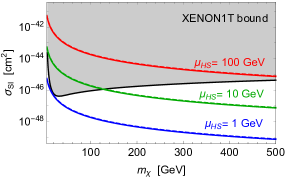
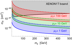
Figure 1: The spin-independent DM–nucleus interaction cross section for different parameter values regardless of the relic density of the DM candidate, $\chi$. The cross-section values constrained by the XENON1T experiment Akerib:2016vxi ; Aprile:2018dbl are shown in gray. In each plot, the solid lines represent the cross section for the minimum considered value for $\sin\theta=0.01$ and the dashed lines represent the maximum considered value of $\sin\theta=0.2$. In all plots, $w=250$ GeV, $m_{2}=200$ GeV and the U(1)-breaking parameters which are not shown are set to zero, except for $\mu_{S}^{\prime 2}$.

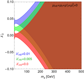
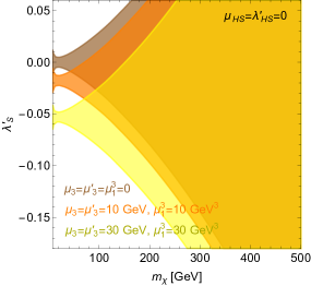
Figure 2: Coloured regions are what is allowed by direct-detection bounds from XENON1T for $\sin\theta=0.1$, regardless of the relic-density contribution of the DM candidate. In the symmetry-breaking potential all terms with odd powers of the singlet have been set to zero in the left panel, and in the right panel all doublet–singlet mixing terms have been set to zero. In both panels $w=250$ GeV and $m_{2}=200$ GeV.

3.2 Cancellation regions

Let us study the general formula for the effective direct-detection coupling in the $t\to 0$ limit in eq. (23) in more detail. As noted before, this result is generally non-zero in the presence of any of the symmetry-breaking interactions in eq. (3). However, there are specific combinations of the symmetry-breaking parameters which lead to a suppressed $\lambda_{\rm SI}$ in the $t\to 0$ limit, thereby mimicking the behaviour of the minimal $\mathbb{Z}_{2}$-symmetric model. We shall now explore these cancellation conditions more closely.

Recall first, that in the non-linear representation, if only the U(1)-breaking $\mu_{S}^{\prime 2}$ mass term in eq. (3) is present, we have

$$V_{\mathrm{int}}\supset-\frac{m_{\chi}^{2}}{w}\left[\sin\theta\;h_{1}-\cos\theta\;h_{2}\right]\chi^{2}+\frac{1}{w}\left[\sin\theta\;h_{1}-\cos\theta\;h_{2}\right](\partial_{\mu}\chi)^{2},$$ (24)

yielding the following effective coupling for direct detection, where $p_{1}$ and $k_{1}$ are the momenta of the incoming and outgoing $\chi$-particles, resp.,

$$\lambda_{\mathrm{eff}}^{\mathrm{non-lin}}= \frac{\sin(2\theta)(m_{1}^{2}-m_{2}^{2})}{vw(m_{1}^{2}-t)(m_{2}^{2}-t)}\left(-m_{\chi}^{2}-(-p_{1}\cdot k_{1})\right)$$

$$= \frac{\sin(2\theta)(m_{1}^{2}-m_{2}^{2})}{vw(m_{1}^{2}-t)(m_{2}^{2}-t)}\left(-m_{\chi}^{2}-\frac{1}{2}(t-2m_{\chi}^{2})\right)$$

$$= \ \frac{\sin(2\theta)(m_{1}^{2}-m_{2}^{2})}{vw(m_{1}^{2}-t)(m_{2}^{2}-t)}\left(\frac{-t}{2}\right),$$ (25)

which explicitly shows that the direct-detection cross section vanishes in the $t\to 0$ limit.

Let us now study how the cubics $\mu_{3}$ and $\mu^{\prime}_{3}$ affect the cross section and pseudo-Goldstone mass. For simplicity, we take here $\lambda^{\prime}_{S}=0$ and $\mu^{3}_{1}=0$ and also set all symmetry-breaking terms involving the Higgs boson to zero. Representing the singlet field, $S$, as

$$S=\frac{s+w}{\sqrt{2}}e^{i\chi/w},$$ (26)

the cubic terms in the potential (1) can be written as

$$V_{3}=\frac{1}{2\sqrt{2}}(s+w)^{3}\left[\mu_{3}\cos\left(\frac{3\chi}{w}\right)+\mu_{3}^{\prime}\cos\left(\frac{\chi}{w}\right)\right].$$ (27)

Minimisation of the potential yields

$$\mu_{S}^{2}=-\lambda_{S}w^{2}-\frac{3}{2\sqrt{2}}(\mu_{3}+\mu^{\prime}_{3})w-\mu_{S}^{\prime\,2},$$ (28)

and the mass of $\chi$ is calculated to be

$$m_{\chi}^{2}=-2\mu_{S}^{\prime\,2}-\frac{1}{2\sqrt{2}}(9\mu_{3}+\mu_{3}^{\prime})w.$$ (29)

Let us now try to understand the origin of the contributions to the direct-detection cross section by explicitly relating the derivation of the $\mathbb{Z}_{2}$-symmetric case, eq. (25). The relevant interaction terms in our simplified case are given by

$$\begin{split}V_{\rm int}\supset&-\frac{1}{8w^{2}}\left[8\mu_{S}^{\prime 2}(s+w)^{2}+\sqrt{2}(9\mu_{3}+\mu_{3}^{\prime})(s+w)^{3}\right]\chi^{2}\\ =&-\left[\mu_{S}^{\prime 2}+\frac{1}{4\sqrt{2}}(9\mu_{3}+\mu_{3}^{\prime})w\right]\chi^{2}-\frac{1}{w}\left[2\mu_{S}^{\prime 2}+\frac{3}{4\sqrt{2}}(9\mu_{3}+\mu_{3}^{\prime})w\right]s\chi^{2}+\dots\\ =&\frac{1}{2}m_{\chi}^{2}\chi^{2}+\frac{1}{w}\left[m_{\chi}^{2}-\frac{1}{4\sqrt{2}}(9\mu_{3}+\mu_{3}^{\prime})w\right]s\chi^{2}+\dots,\end{split}$$ (30)

where we used eq. (5) to obtain the last equality. The second term in the parenthesis of the last line of eq. (30) does not cancel by the mass coming from the derivative terms, and thus there is a contribution to direct detection from the cubic terms.

However, note how the mass $m_{\chi}$, given by eq. (29) in the simplified case at hand, is proportional to the same combination of parameters as in the direct-detection cross section. This shows explicitly that also in this case the suppression of the direct-detection rate is tied to the pseudo-Goldstone nature of the $\chi$ field.

In the special case $\mu_{3}^{\prime}=-9\mu_{3}$, when the tree-level direct-detection cross section cancels, the contribution to $m_{\chi}$ from the cubic terms goes to zero as well, thereby implying a more symmetric vacuum than just an accidental cancellation. This can be understood by the form of the $\chi$-potential at the vacuum, eq. (27). To illustrate this explicitly, we show the cubic part of the potential and its derivatives for the special parameter domain $\mu_{3}^{\prime}=-9\mu_{3}$ in figure 3.

Figure 3: The potential, $V_{3}$, and its first two derivatives with respect to $\chi$ at $s=0$ for ${\mu_{3}^{\prime}=-9\mu_{3}}$.

As we noted above, the second derivative of $V_{3}$ with respect to $\chi$ vanishes when evaluated in the vacuum. However, notice that the cubic contributions along the $s$ direction are not zero at $\chi=0$ even for $\mu_{3}^{\prime}=-9\mu_{3}$ implying that the full Lagrangian does not have an enhanced symmetry in this limit.

In the general case of eq. (23), setting the combinations of parameters which appear in the direct-detection cross section,

$$9\mu_{3}+\mu^{\prime}_{3},\qquad 4\mu^{3}_{1}+v^{2}\mu_{HS},\qquad 4w\lambda^{\prime}_{HS}+\mu_{HS},$$ (31)

to zero leads to suppression of the direct-detection rate. It can be shown that these same combinations also appear in $m_{\chi}$. To illustrate these conclusions, we show in the left panel of figure 4 the contours of the ratio of tree-level $\sigma_{\rm{SI}}$ to the XENON1T upper limit on the DM–nucleon cross section for the parameter combination $9\mu_{3}+\mu^{\prime}_{3}$. Thus, contours with values of one or less are allowed. For this plot, we have chosen the typical values of $w=250$ GeV, $m_{2}=200$ GeV and $\sin\theta=0.1$, while all other symmetry-breaking terms (except for $\mu_{S}^{\prime 2}$) are set to zero.

3.3 Direct-detection cross section at one loop

As shown in Azevedo:2018exj , in the case of the simplest U(1)-invariant model broken by only the $\mathbb{Z}_{2}$-symmetric mass term, the non-vanishing corrections to the direct-detection cross section in the $t\to 0$ limit arise at one-loop order. When more general U(1)-breaking interactions are considered, they will yield ${\cal O}(t^{0})$ contributions to the direct-detection cross section already at tree level. The allowed magnitude of these interactions at tree level is expected to be roughly similar to the size of the loop corrections due to the mass term Alanne:2018zjm . The loop corrections arising from the symmetry-breaking interactions are then expected to be negligible.

However, as we have discussed above, the contributions from the symmetry-breaking interactions are suppressed at tree level in specific parts of the parameter space. In such case the effect of loop corrections becomes again relevant. Therefore, we will briefly discuss the one-loop contribution in the presence of these cubic terms extending the analysis of ref. Azevedo:2018exj .

We will concentrate here on the case where the only non-zero cubics are $\mu_{3}$ and $\mu_{3}^{\prime}$. This choice is motivated by simplicity, but also because we want to, in particular, study if the suppression of the direct-detection cross section for the specific choice $\mu_{3}^{\prime}=-9\mu_{3}$ is preserved at the loop level.

The spin-independent cross section with the one-loop corrections at $t\to 0$ limit can be written as

$$\sigma_{\rm SI}=\frac{f_{N}^{2}m_{N}^{2}}{4\pi m_{\chi}^{2}}\left(\frac{m_{\chi}m_{N}}{m_{\chi}+m_{N}}\right)^{2}|\lambda_{\rm SI}^{\rm tree}+\lambda^{\rm 1L}_{\rm SI}|^{2},$$ (32)

where now $\lambda_{\rm SI}^{\rm tree}$ is given by eq. (23) with $\mu_{1}=\mu_{HS}=0\,{\rm GeV}$, and $\lambda_{HS}^{\prime}=\lambda_{S}^{\prime}=0$. In general, $\lambda_{\rm SI}^{\rm 1L}$ has a complicated analytic expression involving several loop functions. In the particular case $\delta\equiv 9\mu_{3}+\mu_{3}^{\prime}=0$ the expression simplifies significantly, and we show the result for illustration in appendix C. In the numerical computation we keep the full expression including the deviation from the $\delta=0$ limit.

While at tree level, the value of only the combination $\delta$ is relevant, at loop level also the individual values of the coupligns $\mu_{3}$ and $\mu_{3}^{\prime}$ become important, since the limit $\delta=0$ does not correspond to a symmetry at the Lagrangian level. We illustrate this in figure 4, where we plot the spin-independent cross section (again regardless of the relic-density contribution) at tree and one-loop levels as a function of $m_{\chi}$ and $\delta$ for two representative values of $\mu_{3}=50,500$ GeV. For the numerical evaluation of the various loop functions, we use the pySecDec toolbox Borowka:2017idc ; Borowka:2018goh with FORM optimization Vermaseren:2000nd ; Kuipers:2013pba ; Ruijl:2017dtg and CUBA library for multi-dimensional integration Hahn:2004fe ; Hahn:2014fua .

Figure 4: Cancellation regions for the DM-nucleon interaction cross section, regardless of the relic density contributions; contours show the value for $\sigma_{\rm SI}$ over the XENON1T limit cross section, $\sigma_{\max}$, meaning that the contours showing a value less than one pass the direct-detection bounds. Here, we have set $w=250$ GeV, $m_{2}=200$ GeV and $\sin\theta=0.1$. Note that all other symmetry-breaking terms not explicitly presented in the plot are set to zero: $\mu_{1}=\mu_{HS}=0$ GeV and $\lambda^{\prime}_{S}=\lambda^{\prime}_{HS}=0$.

Figure 4 shows that the suppression of the direct-detection cross section persists also at one-loop level for moderate values of the couplings $\mu_{3},\mu_{3}^{\prime}$, but at larger values the interference with the symmetry-breaking mass term increases the one-loop cross section significantly at large $m_{\chi}$. Note however, that near the $\delta=0$ region for $\delta<0$ and large $m_{\chi}$, the tree-level and one-loop contributions interfere destructively, allowing for the region of suppressed direct-detection cross section for larger DM masses, too.

We conclude that the situation is analogous to the simplest $\mathbb{Z}_{2}$-symmetric model of pseudo-Goldstone DM: starting from a model in the cancellation region of U(1)-breaking parameters discussed in the previous section, we expect deviation from the symmetric $t\to 0$ limit of the direct-detection cross section by contributions of the order of the loop corrections discussed in this section.

Another feature arising from loop corrections is that the parameter combination $\delta=9\mu_{3}+\mu_{3}^{\prime}$ may not stay zero under running of couplings. The $\beta$-functions of the model are given in appendix D. As a simple example, let us consider the case where all other symmetry-breaking interactions are set to zero except $\mu_{3}$ and $\mu_{3}^{\prime}$. Then we have

$$\begin{split}16\pi^{2}\frac{d(9\mu_{3}+\mu^{\prime}_{3})}{dt}&=12\lambda_{S}(9\mu_{3}+\mu^{\prime}_{3})+8\lambda_{S}\mu^{\prime}_{3},\end{split}$$ (33)

which explicitly shows that the running of $\delta$ is not multiplicative. Generally, the model should be viewed as a low-energy effective theory with the coefficients of the symmetry-breaking operators taking non-zero values constrained to be compatible with experiments and observations. Nevertheless, the cancellation regions we have discussed here may be interesting towards more complete model building, in particular with the relatively large regions of the parameter space near the $\delta=0$ limit with suppressed direct-detection cross section persisting even at one-loop level.

3.4 Indirect detection

Finally, to relate the present analysis to the results of ref. Alanne:2018zjm , we discuss the implications of indirect detection of DM for our model framework. The relevant indirect-detection constraints arise due to annihilation of DM in the dwarf galaxies that orbit our Milky Way. In these structures the DM is cold and therefore DM annihilations take place essentially at vanishing momentum: $s\to 4m_{\chi}^{2}$. The annihilation cross section to all final states, $f\bar{f}$, $W^{+}W^{-}$, $ZZ$, $h_{1}h_{1}$, $h_{1}h_{2}$ and $h_{2}h_{2}$ is non-vanishing in this limit (unless kinematically forbidden). The annihilation cross sections for these processes are given in appendix B.

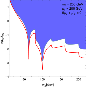
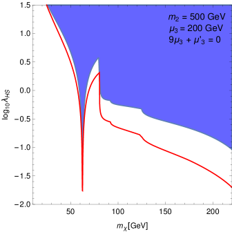
Figure 5: The left panel presents the indirect-detection constraints for $m_{2}=200$ GeV and the right panel for $m_{2}=500$ GeV. In both panels $\sin\theta=0.2$. The red curve shows where the model reproduces the observed relic density, $f_{\rm rel}=1$. The blue area is excluded by the latest Fermi-LAT data Boddy:2019qak . Of the explicit breaking terms, only the mass term $\mu_{S}^{\prime 2}$ and the cubics $\mu_{3}$ and $\mu^{\prime}_{3}$ satisfying $\delta=9\mu_{3}+\mu_{3}^{\prime}=0$ are present.

The constraints from the Fermi-LAT dwarf galaxy observations, based on the recent analysis Boddy:2019qak , are presented in figure 5. The red curve shows where the model reproduces the observed relic density, $f_{\rm rel}=1$. The excluded regions, shown in blue, are produced by comparing the annihilation cross section $v_{\rm rel}\,\sigma_{\chi\chi\to\,b\bar{b}}$ to the reported $b\bar{b}$ exclusion limit for $m_{\chi}<m_{W^{\pm}}$. In the region $m_{\chi}>m_{W^{\pm}}$, the dominant annihilation channel is to $W^{+}W^{-}$ and in this region we compare the total DM annihilation cross section — that is, the combined cross sections $\chi\chi\to W^{+}W^{-},ZZ,h_{1}h_{1},h_{1}h_{2},h_{2}h_{2}$ — to the $W^{+}W^{-}$ bound. The kinks in the plot occur at kinematic thresholds for each channel, that is at ${m_{\chi}=m_{W^{\pm}},m_{Z},m_{1},(m_{1}+m_{2})/2,m_{2}}$. We have set all the explicit U(1)-breaking terms to zero in figure 5, except for the mass term $\mu_{S}^{\prime 2}$ and the cubics $\mu_{3}$ and $\mu^{\prime}_{3}$ satisfying $\delta=9\mu_{3}+\mu_{3}^{\prime}=0$.

The gamma ray flux originating from DM annihilations in a dwarf galaxy depends on the density profile of the DM halo. This effect is described via the so-called $J$-factor. In the present analysis we use the constraints on $\chi\chi\to b\bar{b}$ and $\chi\chi\to W^{+}W^{-}$ cross sections based on $J$-factors obtained in Boddy:2019qak . These updated bounds are weaker than the ones used in our previous work Alanne:2018zjm , and therefore we find the model less constrained by the indirect-detection data. We conclude that, taking into account the uncertainties in the determination of the $J$-factors, the model is not presently constrained by indirect detection in the $m_{\chi}>m_{1}/2$ region.

4 Phase transitions and gravitational waves

4.1 Thermal potential

So far we have seen how the pseudo-Goldstone DM model can account for the observed relic abundance, and how it is constrained by direct-detection experiments. Since the model consists of an extended scalar sector, it is natural to explore the finite-temperature phase transitions in the early universe and their phenomenological consequences, in particular for the GW signals relevant for the LISA, BBO or DECIGO satellites.

It turns out that the phenomenologically viable scenario is a two-step transition starting from the high-temperature vacuum in the singlet direction $(h,s)=(0,w_{0})$. With the linear and the cubic terms present — in the absence of an additional $\mathbb{Z}_{2}$ symmetry — the symmetry in the $s$ direction is not necessarily restored, and $w_{0}$ can be non-zero. In the first step, as temperature is lowered, another minimum forms in the singlet direction, $(h,s)=(0,w_{1})$, and the transition $(0,w_{0})\to(0,w_{1})$ occurs at the critical temperature $T_{c}$. This transition is potentially of first order, and can produce GW signals to be searched for in the future space-based missions. The electroweak transition from $(0,w_{1})$ to $(v_{2},w_{2})$ happens at a significantly lower temperature $T_{c}^{\rm EWPT}\ll T_{c}$, and finally evolves to the zero-temperature global minimum $(v,w)$. In the phenomenologically viable parameter space for DM, this second transition is predominantly of second order, and does not produce detectable GW signals. In the following, we will concentrate on the former first-order transition.

Let us now turn to the quantitative analysis of this scenario. The effective one-loop potential reads

$$V_{\mathrm{eff}}=V_{\mathrm{tree}}+V_{\rm CW}^{0}+V_{\rm 1L}^{T}+V_{\rm CT}\,,$$ (34)

where the tree-level potential is given by eq. (1). The second term, $V_{\rm CW}^{0}$, is the $T=0$ Coleman–Weinberg potential in the $\overline{\rm MS}$ scheme,

$$V_{\rm CW}^{0}=\frac{1}{64\pi^{2}}\sum_{i}(-1)^{F}g_{i}\,M^{4}_{i}(h,s)\left[\ln\frac{M^{2}_{i}(h,s)}{\mu_{0}^{2}}-C_{i}\right],$$ (35)

where $g_{i}$ denotes the number of degrees of freedom, $M_{i}(h,s)$ are the field-dependent masses, and $\mu_{0}$ is the renormalisation scale (which we fix to be $\mu_{0}=v$). In this expression, $F=1$ for fermions and $0$ for bosons, $C_{i}=3/2$ for scalars, fermions and longitudinal polarizations of gauge bosons and $1/2$ for transverse polarizations of gauge bosons.

The one-loop finite-temperature corrections are given by

$$V_{\rm 1L}^{T}=\frac{T^{4}}{2\pi^{2}}\sum_{i}g_{i}\,J_{\pm}\left(\frac{M_{i}(h,s)}{T}\right),\qquad J_{\pm}(x)=\pm\int_{0}^{\infty}\!\mathrm{d}y\ y^{2}\ln\left(1\mp\mathrm{e}^{-\sqrt{x^{2}+y^{2}}}\right)\,,$$ (36)

where the upper signs correspond to bosons and lower signs to fermions.

The last term in eq. (34) contains the finite parts of the counter terms that are fixed such that the scalar vevs and masses remain at their tree-level values at the minimum, eq. (8):

$$V_{\mathrm{CT}}=\delta\mu_{H}^{2}|H^{2}|+\delta\mu_{S}^{2}|S|^{2}+\frac{1}{2}\delta\mu_{S}^{2\,\prime}(S^{2}+S^{*\,2})+\delta\lambda_{H}|H|^{4}+\delta\lambda_{S}|S|^{4}+\delta\lambda_{HS}|S|^{2}|H|^{2}\,,$$ (37)

such that the following renormalization conditions are satisfied:

$$\left.\frac{\partial V_{\mathrm{CT}}}{\partial\varphi_{i}}\right|_{\mathrm{vac}}=-\left.\frac{\partial V_{\rm CW}^{0}}{\partial\varphi_{i}}\right|_{\mathrm{vac}}\,,\quad\left.\frac{\partial^{2}V_{\mathrm{CT}}}{\partial\varphi_{i}\partial\varphi_{j}}\right|_{\mathrm{vac}}=-\left.\frac{\partial^{2}V_{\rm CW}^{0}}{\partial\varphi_{i}\partial\varphi_{j}}\right|_{\mathrm{vac}}\,,\quad\varphi=(h,s).$$ (38)

Finally, we use the thermally improved finite-temperature potential, which is obtained by adding to the field-dependent masses in eqs. (35), (36) the leading thermal corrections (see ref. Kainulainen:2019kyp for a recent discussion):

$$M_{i}^{2}(h,s)\rightarrow M_{i}^{2}(h,s)+c_{i}\,T^{2},$$ (39)

where the coefficients $c_{i}$ are given by

$$c_{h}= (9g^{2}+3g^{\prime\,2}+12y_{t}^{2}+24\lambda_{H}+4\lambda_{HS})/48,$$

$$c_{s}= (2\lambda_{HS}+2\lambda_{HS}^{\prime}+4\lambda_{S})/12,$$ (40)

$$c_{\chi}= (2\lambda_{HS}-2\lambda_{HS}^{\prime}+4\lambda_{S})/12.$$

4.2 Gravitational-wave signal and peak-integrated sensitivity curves

During a first-order phase transition, stochastic GWs are produced via three independent mechanisms: collisions of bubbles (b), sound waves in the plasma (s), and turbulence in the plasma (t). The resulting GW spectra can be approximately written in terms of a peak amplitude, $\Omega^{\rm peak}_{i}$, and a spectral shape, $\mathcal{S}_{i}$ which depends on the peak frequency, $f_{i}$,

$$h^{2}\Omega_{i}\left(f\right)=h^{2}\Omega_{i}^{\text{peak}}\,\mathcal{S}_{i}(f,f_{i})\,.$$ (41)

The peak amplitudes and peak frequencies depend on the characteristics of the phase transition which can be quantified in terms of the nucleation temperature, $T_{n}$, the amount of energy density released relative to the radiation energy density Ellis:2019oqb

$$\alpha\equiv\frac{1}{\rho_{\text{rad}}}\left(\Delta V-\frac{T}{4}\Delta\frac{\mathrm{d}V}{\mathrm{d}T}\right)$$ (42)

characterising the strength of the transition, and in terms of

$$\beta/H_{n}\equiv T_{n}\frac{\mathrm{d}(S/T)}{\mathrm{d}T}\qquad\mbox{with}\quad H_{n}=H(T_{n}),$$ (43)

which gives approximately the inverse duration of the transition Grojean:2006bp . Here, $S$ is the Euclidean action of the bubble solution. The latent heat released during the phase transition is converted with efficiency $\kappa_{\rm b}$ into the kinetic energy of the expanding bubbles, with $\kappa_{\rm s}$ into the sound waves, and with $\kappa_{\rm t}$ into the turbulent motion in the plasma. There is still no consensus in the literature on how latent heat released into the kinetic energy of the plasma, $1-\kappa_{\rm b}$, is subsequently transformed into sound waves and turbulence Caprini:2009yp ; Caprini:2015zlo ; Alves:2018jsw ; Axen:2018zvb ; Ellis:2019oqb ; Guo:2020grp ; here we choose the commonly used estimate for the turbulence fraction $\kappa_{\rm t}=0.1$, and we fix the bubble wall velocity $v_{w}=0.9$.

The peak amplitudes and peak frequencies depend on parameters $v_{w}$ and $\kappa_{i}$ and on the values of functions $\alpha$ and $\beta$ evaluated at the nucleation temperature; explicit formulas for these in the runaway-bubble-in-plasma scenario are given in refs. Caprini:2015zlo ; Ellis:2019oqb along with the spectral shape functions, $\mathcal{S}_{i}$, in terms of the peak frequencies.

The resulting GW signal needs to be compared with the noise spectrum of the experiment under consideration to obtain the signal-to-noise ratio (SNR) Allen:1997ad ; Maggiore:1999vm

$$\rho=\left[n_{\text{det}}\,\frac{t_{\text{obs}}}{s}\int_{f_{\text{min}}}^{f_{\text{max}}}\frac{\mathrm{d}f}{\,\mathrm{Hz}}\left(\frac{h^{2}\Omega_{\text{signal}}(f)}{h^{2}\Omega_{\text{noise}}(f)}\right)^{2}\right]^{1/2}\,,$$ (44)

where $n_{\rm det}=1$ if the experiment consists of just one detector allowing only auto-correlation measurement, while $n_{\rm det}=2$ if it is possible to cross-correlate signals of a detector pair. In the following, we will consider three satellite-borne GW interferometers: LISA Audley:2017drz ; Baker:2019nia , DECIGO Seto:2001qf ; Kawamura:2006up ; Yagi:2011wg ; Isoyama:2018rjb , and BBO Crowder:2005nr ; Corbin:2005ny ; Harry:2006fi with the planned configurations $n_{\rm det}=1$ for LISA and $n_{\rm det}=2$ for DECIGO and BBO. The noise spectra of these experiments are discussed in detail in ref. Schmitz:2020syl .

For the representation of the model parameter points in the GW signal region and the experimental reach of the above interferometers, we adopt the approach of peak-integrated sensitivity (PIS) curves put forward recently in refs. Alanne:2019bsm ; Schmitz:2020syl . The advantage of this approach with respect to the conventional power-law-integrated sensitivity curves Thrane:2013oya is that it allows to represent each parameter point as a single point in the GW signal region and is thus well-suited for the purpose of a general scan of the parameter space to be discussed in the following section.

The key observation is that if the shape of the expected signal is known, as is the case of first-order phase transitions, the integration over the spectral shape can be carried out leaving SNR uniquely determined by the peak energy densities and peak frequencies that depend on the model-specific phase-transition quantities and no longer on the GW frequency. More specifically, the SNR in eq. (44) can be rewritten as

$$\frac{\rho^{2}}{t_{\text{obs}}/\mathrm{yr}}= \left(\frac{h^{2}\Omega^{\text{peak}}_{\text{b}}}{h^{2}\Omega_{\text{PIS}}^{\text{b}}}\right)^{2}+\left(\frac{h^{2}\Omega^{\text{peak}}_{\text{s}}}{h^{2}\Omega_{\text{PIS}}^{\text{s}}}\right)^{2}+\left(\frac{h^{2}\Omega^{\text{peak}}_{\text{t}}}{h^{2}\Omega_{\text{PIS}}^{\text{t}}}\right)^{2}$$ (45)

$$+\Bigg{(}\frac{h^{2}\Omega^{\text{peak}}_{\text{b/s}}}{h^{2}\Omega_{\text{PIS}}^{\text{b/s}}}\Bigg{)}^{2}+\Bigg{(}\frac{h^{2}\Omega^{\text{peak}}_{\text{s/t}}}{h^{2}\Omega_{\text{PIS}}^{\text{s/t}}}\Bigg{)}^{2}+\Bigg{(}\frac{h^{2}\Omega^{\text{peak}}_{\text{b/t}}}{h^{2}\Omega_{\text{PIS}}^{\text{b/t}}}\Bigg{)}^{2}\,,$$

where the integration over the frequency range has already been carried out implicitly:

$$h^{2}\Omega_{\text{PIS}}^{i/j}\equiv\left[(2-\delta_{ij})\,n_{\text{det}}\,1\,\mathrm{yr}\int_{f_{\text{min}}}^{f_{\text{max}}}\mathrm{d}f\>\frac{{\mathcal{S}}_{i}(f)\,{\mathcal{S}}_{j}(f)}{\left(h^{2}\Omega_{\text{noise}}(f)\right)^{2}}\right]^{-1/2}\,,$$ (46)

where $i,j\in\left\{\textrm{b},\textrm{s},\textrm{t}\right\}$ and the mixed peak amplitudes are defined as geometric means,

$$h^{2}\Omega^{\text{peak}}_{i/j}=\left(h^{2}\Omega^{\text{peak}}_{i}\,h^{2}\Omega^{\text{peak}}_{j}\right)^{1/2}\,.$$ (47)

For details of the approach, see refs. Alanne:2019bsm ; Schmitz:2020syl .

4.3 Scan of the parameter space and results

We scan the parameter space with non-zero soft-breaking mass and cubic interactions terms $\mu_{3}$ and $\mu_{3}^{\prime}$. We set the quartic couplings $\lambda^{\prime}_{S}$ and $\lambda^{\prime}_{HS}$ to zero since they need to be very small in any case to satisfy the XENON1T direct-detection bounds. We also set $\mu_{HS}$ to zero as it does not contribute significantly to producing a first-order phase transition in the singlet direction in which we are interested. We also set the linear $\mu_{1}^{3}$ term to zero to reduce unnecessary degeneracy, since it can be eliminated in favour of the cubic couplings, cf. appendix A.1. The parameter ranges we consider are $m_{\chi}\in[30,500]$ GeV, $|\sin\theta|\in[0.01,0.2]$, $m_{2}\in[10,1500]$ GeV, $|\mu_{3}|,|\mu^{\prime}_{3}|\in[0,250]$ GeV and $\mu_{HS}=\lambda^{\prime}_{S}=\lambda^{\prime}_{HS}=0$. To keep the scan denser, we employ a conservative perturbativity bound of $\pi/2$ on the absolute values of the quartic couplings.

To implement the constraints from the relic density, we use the micrOMEGAs code Belanger:2018mqt with model files generated by the FeynRules package Christensen:2008py ; Christensen:2009jx ; Alloul:2013bka . To search for the cosmological phase transitions and compute the nucleation temperature, the tunnelling action between the vacua, as well as the phase-transition quantities $\alpha$ and $\beta$, we employ the CosmoTransitions Wainwright:2011kj code. These results were also checked by our own Mathematica code and using the FindBounce package Guada:2020xnz .

In addition, we perform a separate scan to investigate the effect of the linear term $\mu_{1}^{3}$. In this case, we set $\mu_{3}=\mu^{\prime}_{3}=\mu_{HS}=0$, so they are generated solely from elimination of the tadpoles. This elimination is achieved by shifting the field $s\to s+\sigma$ and then demanding that the linear term of the resulting potential vanishes. The effect of the shift on scalar potential parameters is given in appendix A.1. We parametrise this scan in terms of $\sigma$, not $\mu_{1}^{3}$ to avoid solving a cubic equation. In this scan we consider parameter ranges $|\sigma|\in[0.1,200]$ GeV, $|\lambda^{\prime}_{S}|\in[0,0.001]$, $|\lambda^{\prime}_{HS}|\in[0,0.01]$. We consider the singlet vev in the range $|w|\in[1,1.5\times 10^{5}]\leavevmode\nobreak\ \text{GeV}$ and use it to fit the relic density to the observed value of $\Omega_{c}h^{2}$ within three standard deviations Aghanim:2018eyx . However, this linear term scan does not yield any points with strong first-order phase transition, nor is it particularly distinguishable in the direct-detection plots. For that reason we do not further discuss it separately.

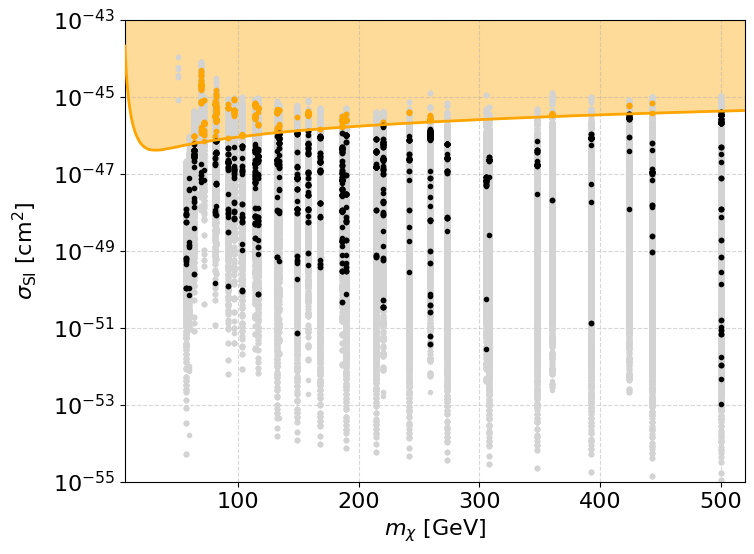
Figure 6: The direct-detection cross section vs. DM mass where the orange shaded region is excluded by the XENON1T experiment. The black and orange points produce a first-order phase transition while the gray points fail to do so. The black points are allowed by the XENON1T bound while the orange points are excluded.

The results of the scan in the plane of direct-detection cross section vs. DM mass are shown in figure 6. The points shown satisfy all theoretical and experimental constraints discussed in section 2 except for the direct-detection bounds by XENON1T which rule out the orange shaded region. The black and orange points produce a first-order phase transition while the gray points fail to do so. The black points are allowed by the XENON1T bound while the orange points are excluded. As is evident from the figure, there are ample regions of the parameter space which provide a viable DM candidate and lead to a first-order phase transition. For these sets of parameters, we then determine the magnitude of the GW signal.

For the stochastic GW background signal, we recast the parameter points into the peak frequency–peak energy density plane, fixing $\kappa_{\rm t}=0.1$. For the PIS curves, we assume the observational time $t_{\rm obs}=4\leavevmode\nobreak\ {\rm yr}$ and threshold SNR $\rho_{\rm thr}=10$ Caprini:2015zlo ; Audley:2017drz for all the experiments. The most sensitive channel turns out to be bubble collisions for which we show the parameter points in the GW signal region in the left panel of figure 7. The black (orange) points are allowed (excluded) by XENON1T constraints.

We observe that obtaining parameter sets which lead to strong enough GW signal observable by future experiments becomes difficult in the generic parameter scan described in the beginning of this section. This is typical for a multi-dimensional parameter space constrained by multiple observables: the viable parameter space becomes more concentrated on lower-dimensional hypersurfaces and refined parameter scanning is needed.

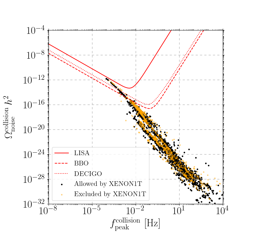
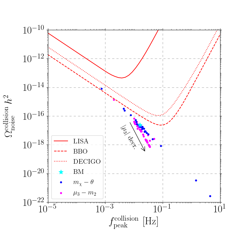
Figure 7: Left panel: Points allowed by the XENON1T experiment in black and points ruled out by it in orange. Right panel: Refined scan around a benchmark (BM) point along the $f_{\rm rel}=1$ hypersurface. The blue points are obtained by varying $m_{\chi}$ and $\theta$ while the magenta points are the result of varying $\mu_{3}$ and $m_{2}$ values.

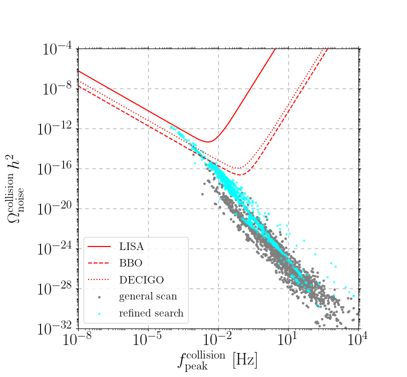
Figure 8: The points from the general scan are shown in gray while the points generated by refined scanning are shown in cyan.

Here, to explore the parameter space for the first-order phase transition more closely, we choose a few viable benchmark points from the general scan and search for more points in their vicinity along $f_{\rm rel}=1$ hypersurfaces varying only two parameters at a time. This search strategy is illustrated in the right panel of figure 7, where we show the variation around a benchmark point

$$(m_{2},m_{\chi},\theta,w,\mu_{3},\mu_{3}^{\prime})=(400\,{\rm GeV},360\,{\rm GeV},0.0316,1320\,{\rm GeV},-200\,{\rm GeV},-3.76\,{\rm GeV})$$

by varying either $(\mu_{3},m_{2})$ or $(m_{\chi},\theta)$. With this refined scan we are able to obtain parameter sets which correspond to models with sufficiently strong first-order transition to be visible in future searches for GWs. To better show the effect of the refined search over the full set of generated points, in figure 8 we show the points from the general scan discussed earlier in gray and the points generated by refined scanning in cyan.

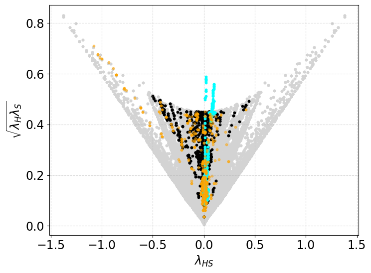
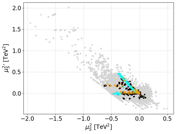
Figure 9: The gray points in both panels show all scanned points while the orange (black) points show the points leading to a first-order phase transition but are excluded (allowed) by XENON1T constraints on the direct-detection cross section. The cyan points are the ones generated by the refined scan.

To complete this discussion, we show how the scanned points are distributed by looking at various projections in the parameter space of the model. In figure 9 the gray points in both panels show all scanned points, while the orange (black) points show the points leading to a first-order phase transition but are excluded (allowed) by XENON1T constraints on the direct-detection cross section. The cyan points are the ones generated by the refined scan.

In the left panel we show the dependence of the scanned points on the portal coupling $\lambda_{HS}$ and on the combination $\sqrt{\lambda_{H}\lambda_{S}}$. The linear envelopes arise from the stability of the potential condition, while the curve bounding the points from above is due to the upper limit $\lambda_{S}=\pi/2$ set by hand to guarantee a conservative bound on perturbativity and unitarity. As expected, the refined points cover very specific regions in the parameter space. Note that in the left panel some of the newly generated points go above the enveloping curve of the general scan. This is merely due to releasing the constraint $\lambda_{S}\leq\pi/2$ slightly but without endangering unitarity. The right panel shows the scanned points with respect to $\mu_{S}^{2}$ and $\mu_{S}^{\prime 2}$.

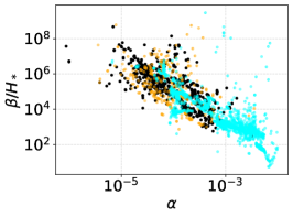
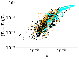
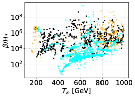
Figure 10: All points leading to a first-order phase transition including the points from the refined scan shown in cyan. The orange (black) points are excluded (allowed) by the XENON1T experiment. Left panel: $\beta/H_{n}$ vs. $\alpha$ at nucleation temperature. Middle panel: $(T_{c}-T_{n})/T_{c}$ vs. $\alpha$. Right panel: $\beta/H_{n}$ vs $T_{n}$.

In figure 10 we show only the points which lead to a first-order phase transition. The orange (black) points are excluded (allowed) by the XENON1T experiment, while all other theoretical and experimental constraints discussed in section 2 are satisfied. The cyan points again correspond to the refined scan. The points are projected into the plane of the quantities relevant for the GW signal. From the plots we see that both $\beta$ and $1-T_{n}/T_{c}$ quantifying the amount of supercooling are correlated with $\alpha$, but the value of $\beta$ and the value of the nucleation temperature are uncorrelated. The refined points follow the same correlation pattern, but the new points are more concentrated towards the region of large $\alpha$.

In figure 11 the same points as in figure 10 are shown, but illustrating the dependence of GW signal on the parameters of the potential. In the left panel we see that the non-zero value of $\mu_{3}$ allows for larger values of $\alpha$. This is expected since a non-zero $\mu_{3}$ contributes to a stronger phase transition. Similarly in the right panel we see that larger nucleation temperature requires a larger absolute value for the vev of the singlet field, $|w|$.

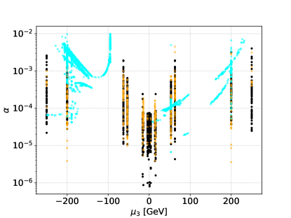
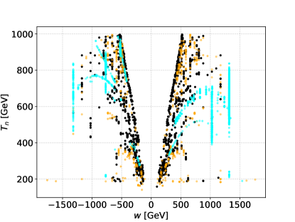
Figure 11: Dependence of phase transition parameters on potential parameters. The points from the refined scan are shown in cyan. The orange points are excluded and the black points are allowed by the XENON1T constraints. All other constraints are satisfied.

This concludes our analysis: we have established the parameter space of the model which provides for the observed DM abundance and is compatible with all present constraints from collider searches and direct and indirect DM detection. Moreover, this same parameter space allows for a first-order phase transition in the early universe whose resulting GW signal may be discovered in future observations.

5 Conclusions

In this paper, we have considered the most general model of pseudo-Goldstone DM that arises from the complex-singlet extension of the SM. Since the global U(1) symmetry is completely broken, the only remaining discrete symmetry is $S\to S^{*}$ which stabilises the imaginary part of the singlet as a DM candidate.

In the $\mathbb{Z}_{2}$-symmetric case, in which the only U(1)-breaking term present is the mass term $\mu_{S}^{\prime 2}$, the tree-level direct-detection cross section vanishes in the $t\to 0$ limit. In the general case, we show that all other U(1)-breaking terms give a non-zero contribution to the direct-detection cross section in the $t\rightarrow 0$ limit significantly increasing the interaction rates relevant for direct-detection experiments and lifting the protection due to the pseudo-Goldstone properties of the DM candidate.

However, we discovered that the symmetry-breaking parameters appear in certain combinations, given explicitly in eq. (31), both in the pseudo-Goldstone mass and the tree-level direct-detection cross section. Setting such combinations to zero leads to cancellations which restore the pseudo-Goldstone properties of the DM candidate and suppress its direct-detection cross section in the $t\rightarrow 0$ limit. Although the running of the couplings upsets this cancellation, the loop-level contributions can be mild and keep the direct-detection cross section moderately suppressed and still interesting from a phenomenological point of view as shown in figure 4. We also considered constraints from indirect detection, but found that they do not presently constrain the parameter space significantly; see figure 5.

We also calculated the finite-temperature effective potential of the model and study the implications for phase transitions in the early universe. We considered a scenario where there is first a first-order transition in the singlet direction $(w,v)=(w_{0},0)\to(w_{1},0)$ with zero Higgs vev $v$, from which a second-order transition brings the fields to the electroweak minimum where both the singlet and the Higgs have non-zero vevs. The barrier in the first transition is generated by the singlet cubic couplings.

Although in most of the parameter space regions the first-order phase transition is not strong enough, we demonstrated that there are regions of the parameter space where a sizeable cubic coupling for a singlet can yield a stochastic GW signal with peak frequency of $10^{-4}$ to $10^{-2}$ Hz which may be detectable by future satellites BBO and DECIGO as illustrated in figure 8. We also established that such couplings also tend to increase the direct-detection signal, and may be observable in future detectors such as the XENONnT experiment. The combination of cubics which suppresses the direct-detection cross section does not yield a strong enough GW signal.

Appendix A Shift of the singlet field

A.1 Shifts of parameters under the shift of the field

We can shift the real part of the complex singlet as $s\to s+\sigma$, e.g., to remove the linear term in the potential. The scalar quartic couplings are shift-invariant, but the dimensionful couplings are shifted as

$$\mu_{1}^{3} \to\mu_{1}^{3}+(\mu^{2}_{S}+\mu^{\prime 2}_{S})\sigma+\frac{3}{2\sqrt{2}}(\mu_{3}+\mu^{\prime}_{3})\sigma+(\lambda_{S}+\lambda^{\prime}_{S}+\lambda^{\prime\prime}_{S})\sigma^{3},$$ (48)

$$\mu_{3} \to\mu_{3}+\frac{1}{\sqrt{2}}(4\lambda^{\prime}_{S}+\lambda^{\prime\prime}_{S})\sigma,$$ (49)

$$\mu^{\prime}_{3} \to\mu^{\prime}_{3}+\frac{1}{\sqrt{2}}(4\lambda_{S}+3\lambda^{\prime\prime}_{S})\sigma,$$ (50)

$$\mu^{2}_{H} \to\mu^{2}_{H}+\frac{1}{2}\mu_{HS}\sigma+\frac{1}{2}(\lambda_{HS}+\lambda^{\prime}_{HS})\sigma^{2},$$ (51)

$$\mu^{2}_{S} \to\mu^{2}_{S}+\sqrt{2}\mu^{\prime}_{3}\sigma+\left(2\lambda_{S}+\frac{3}{2}\lambda^{\prime\prime}_{S}\right)\sigma^{2},$$ (52)

$$\mu^{\prime 2}_{S} \to\mu^{\prime 2}_{S}+\frac{1}{\sqrt{2}}(3\mu_{3}+\mu^{\prime}_{3})\sigma+\left(\lambda_{S}+3\lambda^{\prime}_{S}+\frac{3}{2}\lambda^{\prime\prime}_{S}\right)\sigma^{2}.$$ (53)

A.2 Potential in the shift-invariant notation

In ref. Espinosa:2011ax , the potential of the Higgs boson, $h$, and a real singlet, $s$, is given in terms of shift-invariant quantities. We can extend their formalism to write the potential in eq. (1) of $h$, $s$ and $\chi$ in a shift-invariant way as

$$\begin{split}V&=\frac{m_{h}^{2}}{8v^{2}}(h^{2}-v^{2})^{2}+\left[\frac{m_{sh}^{2}}{2v}(h^{2}-v^{2})+\frac{1}{2}(\lambda_{HI}w+2\mu_{HS})\right](s-w)\\ &+\frac{1}{4}[\lambda_{HR}(h^{2}-v^{2})+2m_{s}^{2}+\lambda_{HI}\chi^{2}](s-w)^{2},\end{split}$$ (54)

where $\lambda_{HR}$ and $\lambda_{HI}$ are defined in eq. (7) and $m_{h}^{2}$, $m_{s}^{2}$ and $m_{sh}^{2}$ are the elements of the CP-even scalar mass matrix. A cosmological constant term appearing with a shift has been omitted.

Appendix B Annihilation cross sections

Here we define the tree-level annihilation cross sections of the pseudo-Goldstone DM, $\chi$. We use short-hand notations $s_{x}\equiv\sin x$, and $c_{x}\equiv\cos x$ for simplicity. It is also useful to define:

$$\beta_{i}=\sqrt{1-\frac{4m_{i}^{2}}{s}},\quad\beta_{ij}=\sqrt{1-\frac{2(m_{i}^{2}+m_{j}^{2})}{s}+\frac{(m_{i}^{2}-m_{j}^{2})^{2}}{s^{2}}},\quad k_{i}=\frac{m_{i}^{2}}{s},$$ (55)

and $v_{\rm rel}=2\beta_{\chi}$.

The annihilation cross section to fermionic final states is

$$\sigma_{\chi\chi\to\bar{f}f}=\frac{N_{c}\beta_{f}^{3}m_{f}^{2}}{\pi v_{\rm rel}v^{2}}\left[\frac{c_{\theta}\lambda_{h_{1}\chi\chi}}{s-m_{1}^{2}}+\frac{s_{\theta}\lambda_{h_{2}\chi\chi}}{s-m_{2}^{2}}\right]^{2},$$ (56)

where the $N_{c}$ is $3$ for quarks and $1$ for leptons.

The annihilation cross sections to gauge boson final states are

$$\sigma_{\chi\chi\to W^{+}W^{-}} =\frac{\beta_{W}}{2\pi v_{\rm rel}sv^{2}}\left[s^{2}-4m_{W}^{2}s+12m_{W}^{4}\right]\left[\frac{c_{\theta}\lambda_{h_{1}\chi\chi}}{s-m_{1}^{2}}+\frac{s_{\theta}\lambda_{h_{2}\chi\chi}}{s-m_{2}^{2}}\right]^{2},$$ (57)

$$\sigma_{\chi\chi\to ZZ} =\frac{\beta_{Z}}{2\pi v_{\rm rel}sv^{2}}\left[s^{2}-4m_{Z}^{2}s+12m_{Z}^{4}\right]\left[\frac{c_{\theta}\lambda_{h_{1}\chi\chi}}{s-m_{1}^{2}}+\frac{s_{\theta}\lambda_{h_{2}\chi\chi}}{s-m_{2}^{2}}\right]^{2}.$$ (58)

The annihilation cross sections to scalar final states are

$$\sigma_{\chi\chi\to h_{i}h_{i}}=\frac{1}{4\pi}\frac{1}{v_{\rm rel}}\frac{\beta_{i}}{s}\Bigg{\{}\alpha^{2}_{i}+\alpha_{i}\frac{8\lambda_{h_{i}\chi\chi}^{2}}{s\beta_{\chi}\beta_{i}}\log\left(\frac{1-2k_{i}+\beta_{\chi}\beta_{i}}{1-2k_{i}-\beta_{\chi}\beta_{i}}\right)$$

$$+\frac{16\lambda_{h_{i}\chi\chi}^{4}}{s^{2}}\left[-\frac{2}{\beta_{\chi}^{2}\beta^{2}_{i}-(1-2k_{i})^{2}}+\frac{1}{\beta_{\chi}\beta_{i}(1-2k_{i})}\log\left(\frac{1-2k_{i}+\beta_{\chi}\beta_{i}}{1-2k_{i}-\beta_{\chi}\beta_{i}}\right)\right]\Bigg{\}},$$ (59)

$$\sigma_{\chi\chi\to h_{1}h_{2}}=\frac{\beta_{12}}{4\pi v_{\rm rel}s}\Bigg{\{}\alpha_{12}^{2}+\alpha_{12}\frac{16\lambda_{h_{1}\chi\chi}\lambda_{h_{2}\chi\chi}}{s\beta_{\chi}\beta_{12}}\log\left(\frac{1-k_{1}-k_{2}+\beta_{\chi}\beta_{12}}{1-k_{1}-k_{2}-\beta_{\chi}\beta_{12}}\right)$$

$$+\frac{32\lambda_{h_{1}\chi\chi}^{2}\lambda_{h_{2}\chi\chi}^{2}}{s^{2}}\left[-\frac{2}{\beta_{\chi}^{2}\beta_{12}^{2}-(1-k_{1}-k_{2})^{2}}\right.$$

$$+\left.\frac{1}{\beta_{\chi}\beta_{12}(1-k_{1}-k_{2})}\log\left(\frac{1-k_{1}-k_{2}+\beta_{\chi}\beta_{12}}{1-k_{1}-k_{2}-\beta_{\chi}\beta_{12}}\right)\right]\Bigg{\}},$$ (60)

where

$$\alpha_{1}=-2\lambda_{h_{1}h_{1}\chi\chi}-\frac{6\lambda_{h_{1}\chi\chi}\lambda_{h_{1}h_{1}h_{1}}}{s-m_{1}^{2}}-\frac{2\lambda_{h_{2}\chi\chi}\lambda_{h_{2}h_{1}h_{1}}}{s-m_{2}^{2}},$$ (61)

$$\alpha_{2}=-2\lambda_{h_{2}h_{2}\chi\chi}-\frac{2\lambda_{h_{1}\chi\chi}\lambda_{h_{1}h_{2}h_{2}}}{s-m_{1}^{2}}-\frac{6\lambda_{h_{2}\chi\chi}\lambda_{h_{2}h_{2}h_{2}}}{s-m_{2}^{2}},$$ (62)

$$\alpha_{12}=-2\lambda_{h_{1}h_{2}\chi\chi}-\frac{2\lambda_{h_{1}\chi\chi}\lambda_{h_{2}h_{1}h_{1}}}{s-m_{1}^{2}}-\frac{2\lambda_{h_{2}\chi\chi}\lambda_{h_{1}h_{2}h_{2}}}{s-m_{2}^{2}}.$$ (63)

The scalar couplings in the above formulae are defined as

$$\lambda_{h_{1}h_{1}\chi\chi}= -\frac{1}{16vw^{3}}\Bigg{[}2vw^{2}(4w\lambda^{\prime}_{HS}+\mu_{HS})c^{2}_{\theta}+4(m_{1}^{2}-m_{2}^{2})w^{2}c^{3}_{\theta}s_{\theta}$$

$$\qquad\quad+v\Big{(}-2(m_{1}^{2}+m_{2}^{2})w+32w^{3}\lambda^{\prime}_{S}-4\mu_{1}^{3}+3\sqrt{2}w^{2}(\mu_{3}+\mu^{\prime}_{3})$$ (64)

$$\qquad\qquad\quad\ -v^{2}\mu_{HS}+2(m_{1}^{2}-m_{2}^{2})wc_{2\theta}\Big{)}s^{2}_{\theta}\Bigg{]}$$

$$\lambda_{h_{2}h_{2}\chi\chi}= -\frac{1}{16vw^{3}}\Bigg{[}2vw^{2}(4w\lambda^{\prime}_{HS}+\mu_{HS})s^{2}_{\theta}+4(m_{1}^{2}-m_{2}^{2})w^{2}c_{\theta}s^{3}_{\theta}$$

$$\qquad\quad+v\Big{(}-2(m_{1}^{2}+m_{2}^{2})w+32w^{3}\lambda^{\prime}_{S}-4\mu_{1}^{3}+3\sqrt{2}w^{2}(\mu_{3}+\mu^{\prime}_{3})$$ (65)

$$\qquad\qquad\quad\ -v^{2}\mu_{HS}+2(m_{1}^{2}-m_{2}^{2})wc_{2\theta}\Big{)}c^{2}_{\theta}\Bigg{]}$$

$$\lambda_{h_{1}h_{2}\chi\chi}= -\frac{c_{\theta}s_{\theta}}{8vw^{3}}\Bigg{[}-2(m_{1}^{2}-m_{2}^{2})vwc_{2\theta}+2(m_{1}^{2}-m_{2}^{2})w^{2}s_{2\theta}$$

$$\qquad\quad+v\Big{(}2(m_{1}^{2}+m_{2}^{2})w+8w^{3}\lambda^{\prime}_{HS}-32w^{3}\lambda^{\prime}_{S}+4\mu_{1}^{3}$$ (66)

$$\qquad\qquad\quad-3\sqrt{2}w^{2}(\mu_{3}+\mu^{\prime}_{3})+v^{2}\mu_{HS}+2w^{2}\mu_{HS}\Big{)}\Bigg{]}$$

$$\lambda_{h_{1}h_{1}h_{1}}= -\frac{1}{16vw^{2}}\Bigg{[}w(-6m_{1}^{2}w+v^{2}\mu_{HS})c_{\theta}-w(2m_{1}^{2}+v^{2}\mu_{HS})c_{3\theta}$$

$$\qquad\quad+2v\Big{(}4m_{1}^{2}w+4\mu_{1}^{3}-\sqrt{2}w^{2}(\mu_{3}+\mu^{\prime}_{s})+v^{2}\mu_{HS}\Big{)}s^{3}_{\theta}\Bigg{]}$$ (67)

$$\lambda_{h_{2}h_{2}h_{2}}= \frac{1}{32vw^{2}}\Bigg{[}3v\Big{(}4m_{2}^{2}w+4\mu_{1}^{3}-\sqrt{2}w^{2}(\mu_{3}+\mu^{\prime}_{3})+v^{2}\mu_{HS}\Big{)}c_{\theta}$$

$$\qquad\qquad\ +v\Big{(}4m_{2}^{2}w+4\mu_{1}^{3}-\sqrt{2}w^{2}(\mu_{3}+\mu^{\prime}_{3})+v^{2}\mu_{HS}\Big{)}c_{3\theta}$$ (68)

$$\qquad\qquad\ -4w\Big{(}-2m_{2}^{2}w+v^{2}\mu_{HS}+(2m_{2}^{2}w+v^{2}\mu_{HS})c_{2\theta}\Big{)}s_{\theta}\Bigg{]}$$

$$\lambda_{h_{1}h_{1}h_{2}}= \frac{s_{\theta}}{16vw^{2}}\Bigg{[}2w(4m_{1}^{2}w+2m_{2}^{2}w+v^{2}\mu_{HS})$$

$$\qquad\qquad\ +2w(4m_{1}^{2}w+2m_{2}^{2}w+3v^{2}\mu_{HS})c_{2\theta}$$ (69)

$$\qquad\qquad\ +v\Big{(}8m_{1}^{2}w+4m_{2}^{2}w+12\mu_{1}^{3}-3\sqrt{2}w^{2}(\mu_{3}+\mu^{\prime}_{3})+3v^{2}\mu_{HS}\Big{)}s_{2\theta}\Bigg{]},$$

$$\lambda_{h_{1}h_{2}h_{2}}= -\frac{c_{\theta}}{16vw^{2}}\Bigg{[}-2w(4m_{2}^{2}w+2m_{1}^{2}w+v^{2}\mu_{HS})+2w(4m_{2}^{2}w+2m_{1}^{2}w+3v^{2}\mu_{HS})c_{2\theta}$$

$$\qquad\quad\ \ +v\Big{(}8m_{2}^{2}w+4m_{1}^{2}w+12\mu_{1}^{3}-3\sqrt{2}w^{2}(\mu_{3}+\mu^{\prime}_{3})+3v^{2}\mu_{HS}\Big{)}s_{2\theta}\Bigg{]}.$$ (70)

Appendix C Direct-detection cross section at one loop

In specific parts of the parameter space, the contributions from the symmetry-breaking interactions are suppressed at tree level. In such case the effect of loop corrections becomes relevant. Therefore, we will briefly discuss how to extend the analysis of ref. Azevedo:2018exj to the case of cubic terms.

Let us first briefly summarize the analysis of ref. Azevedo:2018exj in the U(1)-invariant model with the $\mathbb{Z}_{2}$-symmetric mass term. We write the one-loop contributions to the direct-detection cross section at $t\to 0$ limit as

$$\sigma^{\rm 1L}_{\rm SI}=\frac{f_{N}^{2}m_{N}^{2}}{4\pi m_{\chi}^{2}}\left(\frac{m_{\chi}m_{N}}{m_{\chi}+m_{N}}\right)^{2}|\lambda_{\rm SI}^{\rm 1L}|^{2}$$ (71)

In the absence of other symmetry-breaking operators than the mass term for $\chi$, $\lambda_{\rm SI}^{\rm 1L}$ can be written as

$$\begin{split}\lambda_{\rm SI,\,0}^{\rm 1L}=-\frac{s_{2\theta}(m_{1}^{2}-m_{2}^{2})m_{\chi}^{2}}{4v^{2}w^{3}m_{1}^{2}m_{2}^{2}}&\left[\mathcal{A}_{1}C_{2}(0,m_{\chi}^{2},m_{\chi}^{2},m_{1}^{2},m_{2}^{2},m_{\chi}^{2})\right.\\ &+\mathcal{A}_{2}D_{3}(0,0,m_{\chi}^{2},m_{\chi}^{2},0,m_{\chi}^{2},m_{1}^{2},m_{1}^{2},m_{2}^{2},m_{\chi}^{2})\\ &\left.+\mathcal{A}_{3}D_{3}(0,0,m_{\chi}^{2},m_{\chi}^{2},0,m_{\chi}^{2},m_{1}^{2},m_{2}^{2},m_{2}^{2},m_{\chi}^{2})\right],\end{split}$$ (72)

with short-hand notations $s_{x}\equiv\sin x$ and $c_{x}\equiv\cos x$, and

$$\begin{split}\mathcal{A}_{1}\equiv&4(m_{1}^{2}s_{\theta}^{2}+m_{2}^{2}c_{\theta}^{2})(2m_{1}^{2}vs_{\theta}^{2}+2m_{2}^{2}vc_{\theta}^{2}-m_{1}^{2}ws_{2\theta}+m_{2}^{2}ws_{2\theta}),\\ \mathcal{A}_{2}\equiv&-2m_{1}^{4}s_{\theta}\left[(m_{1}^{2}+5m_{2}^{2})wc_{\theta}-(m_{1}^{2}-m_{2}^{2})(wc_{3\theta}+4vs_{\theta}^{3})\right],\\ \mathcal{A}_{3}\equiv&2m_{2}^{4}c_{\theta}\left[(5m_{1}^{2}+m_{2}^{2})ws_{\theta}-(m_{1}^{2}-m_{2}^{2})(ws_{3\theta}+4vc_{\theta}^{3})\right].\end{split}$$ (73)

Let us then consider what happens in the presence of U(1)-breaking cubic interactions $\frac{1}{2}\mu_{3}(S^{3}+S^{*3})+\frac{1}{2}\mu_{3}^{\prime}SS^{*}(S+S^{*})$. For $\mu_{3}^{\prime}=-9\mu_{3}$, the tree-level direct-detection cross section vanishes in the limit $t\to 0$, so let us write $\mu_{3}^{\prime}=-9\mu_{3}+\delta$. Then

$$\begin{split}\lambda_{\rm SI}^{\rm 1L}=-\frac{s_{2\theta}(m_{1}^{2}-m_{2}^{2})}{4v^{2}w^{3}m_{1}^{2}m_{2}^{2}}&\left[\vphantom{\frac{1}{2}}m_{\chi}^{2}(\mathcal{A}_{1}+\delta_{\mathcal{A}_{1}})C_{2}(0,m_{\chi}^{2},m_{\chi}^{2},m_{1}^{2},m_{2}^{2},m_{\chi}^{2})\right.\\ &+m_{\chi}^{2}(\mathcal{A}_{2}+\delta_{\mathcal{A}_{2}})D_{3}(0,0,m_{\chi}^{2},m_{\chi}^{2},0,m_{\chi}^{2},m_{1}^{2},m_{1}^{2},m_{2}^{2},m_{\chi}^{2})\\ &+m_{\chi}^{2}(\mathcal{A}_{3}+\delta_{\mathcal{A}_{3}})D_{3}(0,0,m_{\chi}^{2},m_{\chi}^{2},0,m_{\chi}^{2},m_{1}^{2},m_{2}^{2},m_{2}^{2},m_{\chi}^{2})\\ &\left.+\mathcal{A}_{4}B_{0}(m_{\chi}^{2},m_{1}^{2},m_{\chi}^{2})+\mathcal{A}_{5}A_{0}(m_{1}^{2})+\mathcal{A}_{6}A_{0}(m_{\chi}^{2})+\mathcal{O}(\delta)\vphantom{\frac{1}{2}}\right],\end{split}$$ (74)

where

$$\begin{split}\delta_{\mathcal{A}_{1}}\equiv&-24\sqrt{2}\mu_{3}(m_{1}^{2}c_{2\theta}-2m_{2}^{2}c_{\theta}^{2})vw+\mathcal{{O}(\delta)},\\ \delta_{\mathcal{A}_{2}}\equiv&\ 24\sqrt{2}\mu_{3}m_{1}^{2}(m_{1}^{2}-m_{2}^{2})vws_{\theta}^{4}+\mathcal{{O}(\delta)},\\ \delta_{\mathcal{A}_{3}}\equiv&-24\sqrt{2}\mu_{3}m_{2}^{2}(m_{1}^{2}-m_{2}^{2})vwc_{\theta}^{4}+\mathcal{{O}(\delta)},\\ \mathcal{A}_{4}\equiv&-12\sqrt{2}\mu_{3}m_{1}^{2}vw+\mathcal{O}(\delta),\\ \mathcal{A}_{5}\equiv&\ 12\sqrt{2}\mu_{3}vw+\mathcal{O}(\delta),\\ \mathcal{A}_{6}\equiv&\ 6\sqrt{2}\mu_{3}vw+\mathcal{O}(\delta).\end{split}$$ (75)

The functions $A_{0}$, $B_{0}$, $C_{2}$ and $D_{3}$ are the standard Passarino-Veltman functions; our definition of these agrees with the ones given in ref. Hahn:1998yk . The last term in eq. (74), $\mathcal{O}(\delta)$, signifies that for $\delta\neq 0$ several additional loop functions appear that cancel out in $\delta=0$ limit. Note that while the divergent parts of the loop functions of coefficients $\mathcal{A}_{4}$ and $\mathcal{A}_{5}$ cancel, the divergent part of the last term $\mathcal{A}_{6}A_{0}(m_{\chi}^{2})$ does not. (Notice, however, that the divergent part vanishes in the limit $m_{\chi}^{2}\to 0$.) A new counter-term of the form $\frac{1}{2}\delta\mu_{3}s\chi^{2}$ is needed, where

$$\delta\mu_{3}=3\sqrt{2}\mu_{3}\frac{A_{0}^{\rm div}(m_{\chi}^{2})}{w^{2}}.$$ (76)

Appendix D Renormalisation group equations

We use the SARAH code Staub:2013tta to calculate the RGEs for the model. For the sake of conciseness, we present here only the one-loop part. Of couplings to fermions, we take into account only the dominant top quark Yukawa coupling of the Higgs boson. The $\beta$-functions for the quartic couplings are given by

$$16\pi^{2}\beta_{\lambda_{H}}= \frac{3}{8}\left(3g^{4}+2g^{2}g^{\prime 2}+g^{\prime 4}\right)-3\lambda_{H}(3g^{2}+g^{\prime 2}-4y_{t}^{2})$$

$$+24\lambda_{H}^{2}+\lambda_{HS}^{2}+\lambda_{HS}^{\prime 2}-6y_{t}^{4},$$ (77)

$$16\pi^{2}\beta_{\lambda_{HS}}= \left[12\lambda_{H}+8\lambda_{S}+4\lambda_{HS}-\frac{3}{2}(3g^{2}+g^{\prime 2})+6y_{t}^{2}\right]\lambda_{HS}+4\lambda_{HS}^{\prime 2}+6\lambda^{\prime}_{HS}\lambda^{\prime\prime}_{S},$$ (78)

$$16\pi^{2}\beta_{\lambda^{\prime}_{HS}}= \left[12\lambda_{H}+4\lambda_{S}+8\lambda_{HS}+12\lambda^{\prime}_{S}-\frac{3}{2}(3g^{2}+g^{\prime 2})+6y_{t}^{2}\right]\lambda^{\prime}_{HS}+6\lambda_{HS}\lambda^{\prime\prime}_{S},$$ (79)

$$16\pi^{2}\beta_{\lambda_{S}}= \,20\lambda_{S}^{2}+36\lambda_{S}^{\prime 2}+\frac{27}{2}\lambda_{S}^{\prime\prime 2}+2\lambda_{HS}^{2}+\lambda_{HS}^{\prime 2},$$ (80)

$$16\pi^{2}\beta_{\lambda^{\prime}_{S}}= \,24\lambda_{S}\lambda^{\prime}_{S}+\frac{9}{2}\lambda_{S}^{\prime\prime 2}+\lambda_{HS}^{\prime 2},$$ (81)

$$16\pi^{2}\beta_{\lambda^{\prime\prime}_{S}}= \,4\lambda_{HS}\lambda^{\prime}_{HS}+36(\lambda_{S}+\lambda^{\prime}_{S})\lambda^{\prime\prime}_{S}.$$ (82)

The $\beta$-functions for the cubic couplings are given by

$$16\pi^{2}\beta_{\mu_{3}}= \,12\lambda_{S}\mu_{3}+6(\lambda^{\prime}_{S}+2\lambda^{\prime\prime}_{S})\mu^{\prime}_{3}+\sqrt{2}\lambda^{\prime}_{HS}\mu_{HS},$$ (83)

$$16\pi^{2}\beta_{\mu^{\prime}_{3}}= \,36\lambda^{\prime}_{S}\mu_{3}+20\lambda_{S}\mu^{\prime}_{3}+6\lambda^{\prime\prime}_{S}(3\mu_{3}+2\mu^{\prime}_{3})+\sqrt{2}(2\lambda_{HS}+\lambda^{\prime}_{HS})\mu_{HS},$$ (84)

$$16\pi^{2}\beta_{\mu_{HS}}= -\frac{3}{4}(g^{\prime 2}+3g^{2})\mu_{HS}+3y_{t}^{2}\mu_{HS}+6\lambda_{H}\mu_{HS}+2\lambda_{HS}(\sqrt{2}\mu^{\prime}_{3}+\mu_{HS})$$

$$+\lambda^{\prime}_{HS}(3\sqrt{2}\mu_{3}+\sqrt{2}\mu^{\prime}_{3}+2\mu_{HS}).$$ (85)

References

- (1) LUX collaboration, D. S. Akerib et al., Results from a search for dark matter in the complete LUX exposure, Phys. Rev. Lett. 118 (2017) 021303 [1608.07648].
- (2) XENON collaboration, E. Aprile et al., Dark Matter Search Results from a One Ton-Year Exposure of XENON1T, Phys. Rev. Lett. 121 (2018) 111302 [1805.12562].
- (3) PandaX-II collaboration, X. Cui et al., Dark Matter Results From 54-Ton-Day Exposure of PandaX-II Experiment, Phys. Rev. Lett. 119 (2017) 181302 [1708.06917].
- (4) C. Gross, O. Lebedev and T. Toma, Cancellation Mechanism for Dark-Matter–Nucleon Interaction, Phys. Rev. Lett. 119 (2017) 191801 [1708.02253].
- (5) K. Huitu, N. Koivunen, O. Lebedev, S. Mondal and T. Toma, Probing pseudo-Goldstone dark matter at the LHC, Phys. Rev. D100 (2019) 015009 [1812.05952].
- (6) T. Alanne, M. Heikinheimo, V. Keus, N. Koivunen and K. Tuominen, Direct and indirect probes of Goldstone dark matter, Phys. Rev. D99 (2019) 075028 [1812.05996].
- (7) D. Azevedo, M. Duch, B. Grzadkowski, D. Huang, M. Iglicki and R. Santos, Testing scalar versus vector dark matter, Phys. Rev. D99 (2019) 015017 [1808.01598].
- (8) D. Karamitros, Pseudo Nambu-Goldstone Dark Matter: Examples of Vanishing Direct Detection Cross Section, Phys. Rev. D 99 (2019) 095036 [1901.09751].
- (9) J. M. Cline and T. Toma, Pseudo-Goldstone dark matter confronts cosmic ray and collider anomalies, Phys. Rev. D100 (2019) 035023 [1906.02175].
- (10) C. Arina, A. Beniwal, C. Degrande, J. Heisig and A. Scaffidi, Global fit of pseudo-Nambu-Goldstone Dark Matter, JHEP 04 (2020) 015 [1912.04008].
- (11) V. Barger, P. Langacker, M. McCaskey, M. Ramsey-Musolf and G. Shaughnessy, Complex Singlet Extension of the Standard Model, Phys. Rev. D79 (2009) 015018 [0811.0393].
- (12) C.-W. Chiang, M. J. Ramsey-Musolf and E. Senaha, Standard Model with a Complex Scalar Singlet: Cosmological Implications and Theoretical Considerations, Phys. Rev. D97 (2018) 015005 [1707.09960].
- (13) K. Kannike and M. Raidal, Phase Transitions and Gravitational Wave Tests of Pseudo-Goldstone Dark Matter in the Softly Broken U(1) Scalar Singlet Model, Phys. Rev. D99 (2019) 115010 [1901.03333].
- (14) K. Kannike, K. Loos and M. Raidal, Gravitational wave signals of pseudo-Goldstone dark matter in the complex singlet model, Phys. Rev. D101 (2020) 035001 [1907.13136].
- (15) E. Witten, Cosmic Separation of Phases, Phys. Rev. D30 (1984) 272.
- (16) C. J. Hogan, NUCLEATION OF COSMOLOGICAL PHASE TRANSITIONS, Phys. Lett. 133B (1983) 172.
- (17) P. J. Steinhardt, Relativistic Detonation Waves and Bubble Growth in False Vacuum Decay, Phys. Rev. D25 (1982) 2074.
- (18) LISA collaboration, P. Amaro-Seoane et al., Laser Interferometer Space Antenna, 1702.00786.
- (19) J. Baker et al., The Laser Interferometer Space Antenna: Unveiling the Millihertz Gravitational Wave Sky, 1907.06482.
- (20) N. Seto, S. Kawamura and T. Nakamura, Possibility of direct measurement of the acceleration of the universe using 0.1-Hz band laser interferometer gravitational wave antenna in space, Phys. Rev. Lett. 87 (2001) 221103 [astro-ph/0108011].
- (21) S. Kawamura et al., The Japanese space gravitational wave antenna DECIGO, Class. Quant. Grav. 23 (2006) S125.
- (22) K. Yagi and N. Seto, Detector configuration of DECIGO/BBO and identification of cosmological neutron-star binaries, Phys. Rev. D83 (2011) 044011 [1101.3940].
- (23) S. Isoyama, H. Nakano and T. Nakamura, Multiband Gravitational-Wave Astronomy: Observing binary inspirals with a decihertz detector, B-DECIGO, PTEP 2018 (2018) 073E01 [1802.06977].
- (24) J. Crowder and N. J. Cornish, Beyond LISA: Exploring future gravitational wave missions, Phys. Rev. D72 (2005) 083005 [gr-qc/0506015].
- (25) V. Corbin and N. J. Cornish, Detecting the cosmic gravitational wave background with the big bang observer, Class. Quant. Grav. 23 (2006) 2435 [gr-qc/0512039].
- (26) G. M. Harry, P. Fritschel, D. A. Shaddock, W. Folkner and E. S. Phinney, Laser interferometry for the big bang observer, Class. Quant. Grav. 23 (2006) 4887.
- (27) M. Jiang, L. Bian, W. Huang and J. Shu, Impact of a complex singlet: Electroweak baryogenesis and dark matter, Phys. Rev. D93 (2016) 065032 [1502.07574].
- (28) A. Alves, T. Ghosh, H.-K. Guo and K. Sinha, Resonant Di-Higgs Production at Gravitational Wave Benchmarks: A Collider Study using Machine Learning, JHEP 12 (2018) 070 [1808.08974].
- (29) A. Alves, T. Ghosh, H.-K. Guo, K. Sinha and D. Vagie, Collider and Gravitational Wave Complementarity in Exploring the Singlet Extension of the Standard Model, JHEP 04 (2019) 052 [1812.09333].
- (30) D. Azevedo, M. Duch, B. Grzadkowski, D. Huang, M. Iglicki and R. Santos, One-loop contribution to dark-matter-nucleon scattering in the pseudo-scalar dark matter model, JHEP 01 (2019) 138 [1810.06105].
- (31) K. Ishiwata and T. Toma, Probing pseudo Nambu-Goldstone boson dark matter at loop level, JHEP 12 (2018) 089 [1810.08139].
- (32) W. Chao, H.-K. Guo and J. Shu, Gravitational Wave Signals of Electroweak Phase Transition Triggered by Dark Matter, JCAP 09 (2017) 009 [1702.02698].
- (33) G. C. Branco, L. Lavoura and J. P. Silva, CP Violation, Int. Ser. Monogr. Phys. 103 (1999) 1.
- (34) K. Kannike, Vacuum Stability Conditions From Copositivity Criteria, Eur. Phys. J. C72 (2012) 2093 [1205.3781].
- (35) K. Kannike, Vacuum Stability of a General Scalar Potential of a Few Fields, Eur. Phys. J. C76 (2016) 324 [1603.02680].
- (36) S. Kanemura, T. Kubota and E. Takasugi, Lee-Quigg-Thacker bounds for Higgs boson masses in a two doublet model, Phys. Lett. B313 (1993) 155 [hep-ph/9303263].
- (37) A. G. Akeroyd, A. Arhrib and E.-M. Naimi, Note on tree level unitarity in the general two Higgs doublet model, Phys. Lett. B490 (2000) 119 [hep-ph/0006035].
- (38) M. D. Goodsell and F. Staub, Unitarity constraints on general scalar couplings with SARAH, Eur. Phys. J. C78 (2018) 649 [1805.07306].
- (39) P. A. Samuelson, How deviant can you be?, Journal of the American Statistical Association 63 (1968) 1522.
- (40) G. Bélanger, K. Kannike, A. Pukhov and M. Raidal, Minimal semi-annihilating scalar dark matter, JCAP 1406 (2014) 021 [1403.4960].
- (41) ATLAS, CMS collaboration, G. Aad et al., Measurements of the Higgs boson production and decay rates and constraints on its couplings from a combined ATLAS and CMS analysis of the LHC pp collision data at and 8 TeV, JHEP 08 (2016) 045 [1606.02266].
- (42) J. Beacham et al., Physics Beyond Colliders at CERN: Beyond the Standard Model Working Group Report, J. Phys. G47 (2020) 010501 [1901.09966].
- (43) CMS collaboration, A. M. Sirunyan et al., Measurements of the Higgs boson width and anomalous couplings from on-shell and off-shell production in the four-lepton final state, Phys. Rev. D99 (2019) 112003 [1901.00174].
- (44) CMS collaboration, V. Khachatryan et al., Searches for invisible decays of the Higgs boson in pp collisions at = 7, 8, and 13 TeV, JHEP 02 (2017) 135 [1610.09218].
- (45) ATLAS collaboration, Combined measurements of Higgs boson production and decay using up to 80 fb-1 of proton–proton collision data at 13 TeV collected with the ATLAS experiment, .
- (46) Planck collaboration, N. Aghanim et al., Planck 2018 results. VI. Cosmological parameters, 1807.06209.
- (47) J. M. Alarcon, J. Martin Camalich and J. A. Oller, The chiral representation of the scattering amplitude and the pion-nucleon sigma term, Phys. Rev. D85 (2012) 051503 [1110.3797].
- (48) J. M. Alarcon, L. S. Geng, J. Martin Camalich and J. A. Oller, The strangeness content of the nucleon from effective field theory and phenomenology, Phys. Lett. B730 (2014) 342 [1209.2870].
- (49) J. M. Cline, K. Kainulainen, P. Scott and C. Weniger, Update on scalar singlet dark matter, Phys. Rev. D88 (2013) 055025 [1306.4710].
- (50) S. Borowka, G. Heinrich, S. Jahn, S. P. Jones, M. Kerner, J. Schlenk et al., pySecDec: a toolbox for the numerical evaluation of multi-scale integrals, Comput. Phys. Commun. 222 (2018) 313 [1703.09692].
- (51) S. Borowka, G. Heinrich, S. Jahn, S. P. Jones, M. Kerner and J. Schlenk, A GPU compatible quasi-Monte Carlo integrator interfaced to pySecDec, Comput. Phys. Commun. 240 (2019) 120 [1811.11720].
- (52) J. A. M. Vermaseren, New features of FORM, math-ph/0010025.
- (53) J. Kuipers, T. Ueda and J. A. M. Vermaseren, Code Optimization in FORM, Comput. Phys. Commun. 189 (2015) 1 [1310.7007].
- (54) B. Ruijl, T. Ueda and J. Vermaseren, FORM version 4.2, 1707.06453.
- (55) T. Hahn, CUBA: A Library for multidimensional numerical integration, Comput. Phys. Commun. 168 (2005) 78 [hep-ph/0404043].
- (56) T. Hahn, Concurrent Cuba, J. Phys. Conf. Ser. 608 (2015) 012066 [1408.6373].
- (57) K. K. Boddy, J. Kumar, A. B. Pace, J. Runburg and L. E. Strigari, Effective -factors for Milky Way dwarf spheroidal galaxies with velocity-dependent annihilation, Phys. Rev. D102 (2020) 023029 [1909.13197].
- (58) Fermi-LAT, DES collaboration, A. Albert et al., Searching for Dark Matter Annihilation in Recently Discovered Milky Way Satellites with Fermi-LAT, Astrophys. J. 834 (2017) 110 [1611.03184].
- (59) S. J. Clark, B. Dutta and L. E. Strigari, Dark Matter Annihilation into Four-Body Final States and Implications for the AMS Antiproton Excess, Phys. Rev. D97 (2018) 023003 [1709.07410].
- (60) K. Boddy, J. Kumar, D. Marfatia and P. Sandick, Model-independent constraints on dark matter annihilation in dwarf spheroidal galaxies, Phys. Rev. D97 (2018) 095031 [1802.03826].
- (61) K. Kainulainen, V. Keus, L. Niemi, K. Rummukainen, T. V. I. Tenkanen and V. Vaskonen, On the validity of perturbative studies of the electroweak phase transition in the Two Higgs Doublet model, JHEP 06 (2019) 075 [1904.01329].
- (62) J. Ellis, M. Lewicki, J. M. No and V. Vaskonen, Gravitational wave energy budget in strongly supercooled phase transitions, JCAP 1906 (2019) 024 [1903.09642].
- (63) C. Grojean and G. Servant, Gravitational Waves from Phase Transitions at the Electroweak Scale and Beyond, Phys. Rev. D75 (2007) 043507 [hep-ph/0607107].
- (64) C. Caprini, R. Durrer and G. Servant, The stochastic gravitational wave background from turbulence and magnetic fields generated by a first-order phase transition, JCAP 0912 (2009) 024 [0909.0622].
- (65) C. Caprini et al., Science with the space-based interferometer eLISA. II: Gravitational waves from cosmological phase transitions, JCAP 1604 (2016) 001 [1512.06239].
- (66) M. Fitz Axen, S. Banagiri, A. Matas, C. Caprini and V. Mandic, Multiwavelength observations of cosmological phase transitions using LISA and Cosmic Explorer, Phys. Rev. D98 (2018) 103508 [1806.02500].
- (67) H.-K. Guo, K. Sinha, D. Vagie and G. White, Phase Transitions in an Expanding Universe: Stochastic Gravitational Waves in Standard and Non-Standard Histories, 2007.08537.
- (68) B. Allen and J. D. Romano, Detecting a stochastic background of gravitational radiation: Signal processing strategies and sensitivities, Phys. Rev. D59 (1999) 102001 [gr-qc/9710117].
- (69) M. Maggiore, Gravitational wave experiments and early universe cosmology, Phys. Rept. 331 (2000) 283 [gr-qc/9909001].
- (70) K. Schmitz, New Sensitivity Curves for Gravitational-Wave Experiments, 2002.04615.
- (71) T. Alanne, T. Hugle, M. Platscher and K. Schmitz, A fresh look at the gravitational-wave signal from cosmological phase transitions, JHEP 03 (2020) 004 [1909.11356].
- (72) E. Thrane and J. D. Romano, Sensitivity curves for searches for gravitational-wave backgrounds, Phys. Rev. D88 (2013) 124032 [1310.5300].
- (73) G. Bélanger, F. Boudjema, A. Goudelis, A. Pukhov and B. Zaldivar, micrOMEGAs5.0 : Freeze-in, Comput. Phys. Commun. 231 (2018) 173 [1801.03509].
- (74) N. D. Christensen and C. Duhr, FeynRules - Feynman rules made easy, Comput. Phys. Commun. 180 (2009) 1614 [0806.4194].
- (75) N. D. Christensen, P. de Aquino, C. Degrande, C. Duhr, B. Fuks, M. Herquet et al., A Comprehensive approach to new physics simulations, Eur. Phys. J. C71 (2011) 1541 [0906.2474].
- (76) A. Alloul, N. D. Christensen, C. Degrande, C. Duhr and B. Fuks, FeynRules 2.0 - A complete toolbox for tree-level phenomenology, Comput. Phys. Commun. 185 (2014) 2250 [1310.1921].
- (77) C. L. Wainwright, CosmoTransitions: Computing Cosmological Phase Transition Temperatures and Bubble Profiles with Multiple Fields, Comput. Phys. Commun. 183 (2012) 2006 [1109.4189].
- (78) V. Guada, M. Nemevšek and M. Pintar, FindBounce: package for multi-field bounce actions, Comput. Phys. Commun. 256 (2020) 107480 [2002.00881].
- (79) J. R. Espinosa, T. Konstandin and F. Riva, Strong Electroweak Phase Transitions in the Standard Model with a Singlet, Nucl. Phys. B854 (2012) 592 [1107.5441].
- (80) T. Hahn and M. Perez-Victoria, Automatized one loop calculations in four-dimensions and D-dimensions, Comput. Phys. Commun. 118 (1999) 153 [hep-ph/9807565].
- (81) F. Staub, SARAH 4 : A tool for (not only SUSY) model builders, Comput. Phys. Commun. 185 (2014) 1773 [1309.7223].