A framework for modelling Molecular Interaction Maps

Abstract

Metabolic networks, formed by a series of metabolic pathways, are made of intracellular and extracellular reactions that determine the biochemical properties of a cell, and by a set of interactions that guide and regulate the activity of these reactions. Most of these pathways are formed by an intricate and complex network of chain reactions, and can be represented in a human readable form using graphs which describe the cell cycle checkpoint pathways.

This paper proposes a method to represent Molecular Interaction Maps (graphical representations of complex metabolic networks) in Linear Temporal Logic. The logical representation of such networks allows one to reason about them, in order to check, for instance, whether a graph satisfies a given property $\phi$, as well as to find out which initial conditons would guarantee $\phi$, or else how can the the graph be updated in order to satisfy $\phi$.

Both the translation and resolution methods have been implemented in a tool capable of addressing such questions thanks to a reduction to propositional logic which allows exploiting classical SAT solvers.

1 Introduction

Metabolic networks, formed by a series of metabolic pathways, are made of intracellular and extracellular reactions that determine the biochemical properties of a cell by consuming and producing proteins, and by a set of interactions that guide and regulate the activity of such reactions. Cancer, for example, can sometimes appear in a cell as a result of some pathology in a metabolic pathway. These reactions are at the center of a cell’s existence, and are regulated by other proteins, which can either activate these reactions or inhibit them. These pathways form an intricate and complex network of chain reactions, and can be represented in a human readable form using graphs, called Molecular Interaction Maps (MIMs) [26, 33] which describe the cell cycle checkpoint pathways (see for instance Figure 1).

Figure 1: atm-chk2/atr-chk1 molecular interaction map.

Although capital for Knowledge Representation (KR) in biology, MIMs are difficult to use due to the very large number of elements they may involve and the intrinsic expertise needed to understand them. Moreover, the lack of a formal semantics for MIMs makes it difficult to support reasoning tasks commonly carried out by experts, such as checking properties on MIMs, determining how a MIM can explain a given property or how a MIM can be updated in order to describe empirically obtained evidences.

This contribution carries on the research undertaken by the authors aiming at providing a formal background to study MIMs. A first set of works proposed a formalisation of MIMs based on a decidable fragment of first-order logic [14, 15, 16]. In an attempt to find a simpler representation, without resorting to the expressivity of first-order logic, other works [1, 2, 3] proposed an ad-hoc defined non-monotonic logic, called Molecular Interaction Logic (MIL), allowing one to formalize the notions of production and consumption of reactives. In order to formalise the “temporal evolution” of a biological system, MIL formulae are then mapped into Linear Temporal Logic (LTL) [32].

This paper embraces the idea, proposed by the above mentioned works, that LTL is a suitable framework for modelling biological systems due to its ability to describe the interaction between components (represented by propositional variables) and their presence/absence in different time instants. Beyond giving a formal definition of graphs representing MIMs, the paper shows how they can be modeled as an LTL theory, by means of a direct “encoding”, without resorting to intermediate (and cumbersome) ad-hoc logics. The logical encoding allows one to formally address reasoning tasks, such as, for instance, checking whether a graph satisfies some given property $\phi$, as well as finding out which initial conditions would guarantee $\phi$, or else how can the the graph be updated in order to satisfy $\phi$. A first prototypal system has been implemented on the basis of the theoretical work, allowing one to automatically accomplish reasoning tasks on MIMs.

It is worth pointing out that the adequacy of LTL to model MIMs is due to the fact that the latter are qualitative representations of biological processes. In other terms, they model the interactions among the different components of a biological system without resorting, for instance, to differential equations like the Systems Biology Markup Language (SBML) [22] does.

The rest of this paper is organized as follows. Section 2 gives a brief overview of modelling approaches for networks of biological entities. Section 3 presents the lac operon that will be used as a leading example to introduce all the concepts dealt with by our approach. Section 4 describes the fundamental elements and concepts of the modelling approach. Section 5 presents Molecular Interaction Graphs (MIGs), which formalize Molecular Interaction Maps capable of describing and reasoning about general pathways. Section 6 explains how MIGs can be represented by use of Linear Temporal Logic. Section 8 describes the current state of the operational implementation of the software tool and section 9 presents some examples on larger problems. Finally, Section 10 concludes this paper and discusses possible future work.

2 Logical Approaches to Biological Systems

The typical objects to be modelled in the framework of systems biology are networks of interacting elements that evolve in time. According to the features of the network and its properties, various approaches can be followed, which can describe the dynamics of the system taking the following elements into consideration:

• Components: they are represented by variables, which can be either discrete or continuous depending on the requirements of the model.

• Interactions: they are represented by rules that specify the dynamical changes in the variables values. These interactions can in their turn be classified according to the adopted representation of time (discrete or continuous). Finally, the execution of an action can be either stochastic or not, if a certain degree of uncertainty is considered, reflecting the assumption of a noisy environment.

According to the different possible semantics, the various modelling approaches may be classified as follows [20]:

• Models that involve component quantities and deterministic interactions: such models are mathematical, inherently quantitative and usually based on ordinary differential equations. Tools like Timed Automata representations or Continuous-Time Markov Chains are used in the construction of models of this category.

• Discrete-value models: they are characterised by the use of discrete time. Approaches like executable models based on Finite State Machines representations or stochastic models such as Discrete-Time Markov Chains belong to this category.

Other hybrid models such as Hybrid Automata or Process Algebraic Techniques, mix discrete and continuous representation for both variables and time dynamics. Biological properties can be distinguished between qualitative and quantitative: in the former case, time has an implicit consideration while the latter involves reasoning on the dynamics of the system along time. To give an example, reachability and temporal ordering of events are considered qualitative properties while equilibrium states and matabolite dynamics are quantitative properties.

Gene Regulatory Networks (GRNs) have been very well studied in the temporal context because the interaction between components may be easily represented by their presence/absence, i.e components are represented by boolean variables and interactions are represented by logical rules on their values. Following this approach Chabrier et al. [10] successfully modeled a very large network, involving more than 500 genes. They resorted to Concurrent Transition Systems (CTS), allowing one to model modular systems, and can be then translated into the NuSMV language. They checked reachability, stability and temporal ordering properties by the use of CTL. A similar study on a much smaller (although real) biological system has been performed in [6]. Here the LTL specification syntax and the Spin model checker are used to verify stability properties.

When a quantitative approach is chosen, the model dimensions drop drastically. This is essentially due to lack of knowledge on the parameter values for all the interactions, and to the increased computational complexity deriving from a large model. In this kind of settings, logical approaches have been used to verify temporal properties on the representations. For instance, [4, 18, 17] use CTL to verify, among other properties, reachability and stability on different types of biological networks, and in  [7] such properties are checked by using LTL. All these approaches are supported not only for theoretical results but also for tools and frameworks that allow biologists to describe a biological network and then verify whether such representations satisfy some desired properties. Among others, the systems BIOCHAM [8], Bio-PEPA [12, 30] and ANIMO [36] are very popular in the community. We refer the reader to [35, 19] for an overview on this topic.

Some considerations can be made from the study of the aforementioned contributions:

• the size of the modelled systems is generally very small, and a great degree of abstraction and suitable tools are needed to deal with large models;

• qualitative approaches are generally enough to analyse a large variety of interesting biological properties;

• temporal logic plays an important role in the representation and verification of biological systems.

Contrarily to approaches incorporating quantitative information into the temporal formalisation [11], our contribution belongs to the category of qualitative approaches, since quantitative information in biological relations, such as the quantity of reactives and their speed of consumption in a reaction, are not formalised. MIMs in fact represent the interaction among the different components of the system and how they evolve in time according to the different reactions. To the best of our knowledge, there is not any contribution where MIMs are used to model quantitative biological information.

3 A simple example: the lac operon

This section describes a simple example, which represents the regulation of the lac operon (lactose operon), already used in [1, 3]. The lac operon is an operon required for the transport and metabolism of lactose in many bacteria. Although glucose is the preferred carbon source for most bacteria, the lac operon allows for the effective digestion of lactose when glucose is not available. The lac operon is a sequence of three genes (lacZ, lacY and lacA) which encodes 3 enzymes which in turn carry the transformation of lactose into glucose. We will concentrate here on lacZ which encodes $\beta$-galactosidase which cleaves lactose into glucose and galactose.

The lac operon uses a two-part control mechanism to ensure that the cell expends energy producing the enzymes encoded by the lac operon only when necessary. First, in the absence of lactose, the lac repressor halts production of the enzymes encoded by the lac operon. Second, in the presence of glucose, the catabolite activator protein (CAP), required for production of the enzymes, remains inactive.

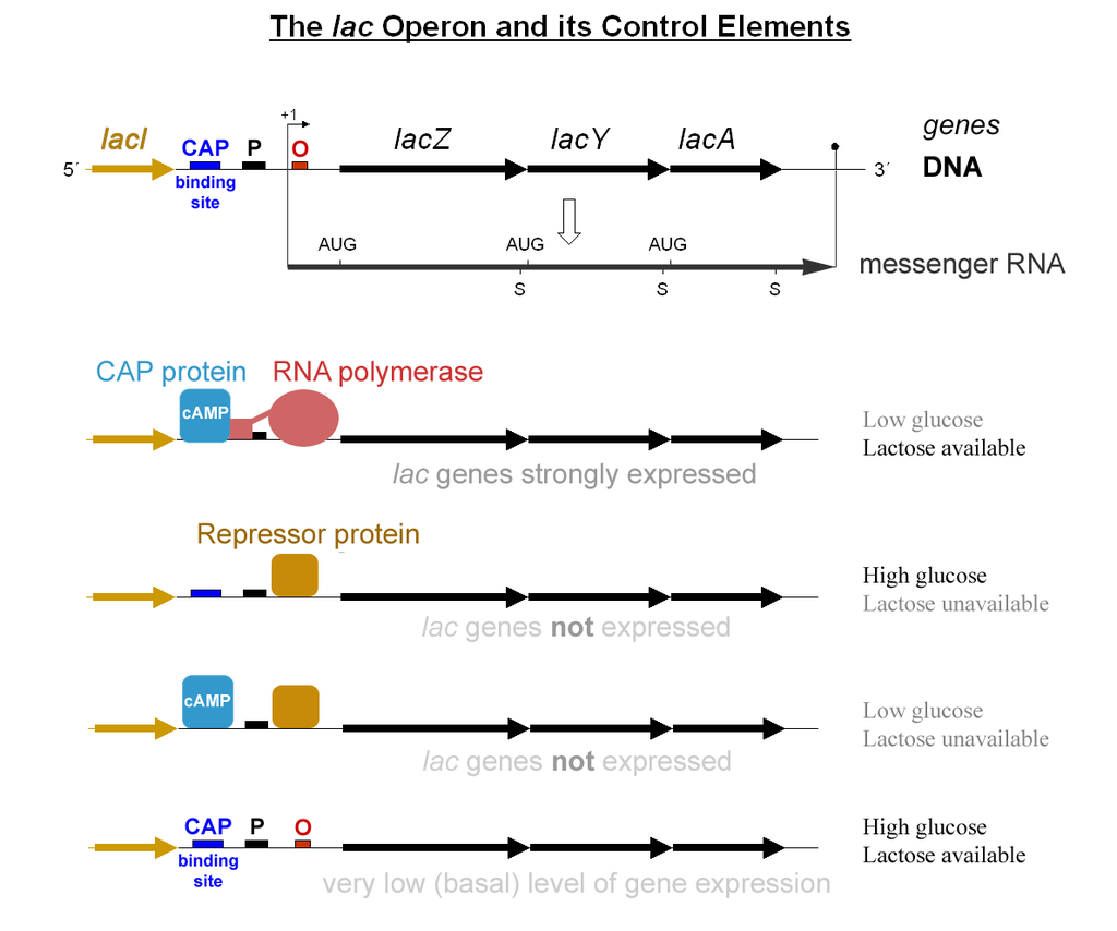
Figure 2: The lac operon

Figure 2 describes this regulatory mechanism. The expression of lacZ gene is only possible when RNA polymerase (pink) can bind to a promotor site (marked P, black) upstream the gene. This binding is aided by the cyclic adenosine monophosphate (CAMP protein, in blue) which binds before the promotor on the CAP site (dark blue).

The lacl gene (yellow) encodes the repressor protein Lacl (yellow) which binds to the promotor site of the RNA polymerase when lactose is not available, preventing the RNA polymerase to bind to the promoter and thus blocking the expression of the following genes (lacZ, lacY and lacA): this is a negative regulation, or inhibition, as it blocks the production of the proteins. When lactose is present, one of its isomer, allolactose, binds with repressor protein Lacl which is no longer able to bind to the promotor site, thus enabling RNA polymerase to bind to the promotor site and to start expressing the lacZ gene if CAMP is bound to CAP.

The CAMP molecule is on the opposite a positive regulation molecule, or an activation molecule, as its presence is necessary to express the lacZ gene. However, the concentration of CAMP is itself regulated negatively by glucose: when glucose is present, the concentration of CAMP becomes low, and thus CAMP does not bind to the CAP site, blocking the expression of lacZ. Thus glucose prevents the activation by CAMP of the expression of galactosidase from lacZ.

4 Molecular Interaction Maps (MIMs)

The mechanism described in the previous section is represented in Figure 3, which is an example of MIM.

Figure 3: Functional representation of the lac operon

This example contains all the relations and all the categories of entities (i.e. the nodes of the graph) that we use in our modelling. They are presented below.

4.1 Relations

The relations among the entities (represented by links in the graphs) represent reactions and can be of different types:

Productions

can take two different forms, depending on whether the reactants are consumed by the reactions or not:

1. The graphical notation used when a reaction consumes completely the reactant(s) is $a_{1},\dots,a_{n}\rightarrowTriangle b$, meaning that the production of $b$ completely consumes $a_{1},\dots,a_{n}$.

   For instance, in Figure 3, lactose, when activated by galactosidase produces glucose, and is consumed while doing so, which is thus noted by $lactose\rightarrowTriangle glucose$.

2. If the reactants are not completely consumed by the reaction, the used notation is $a_{1},\dots,a_{n}\rightarrowtriangle b$. Here $b$ is produced but $a_{1},\dots,a_{n}$ are still present after the production of $b$.

   For example, the expression of the lacZ gene to produce galactosidase (or of the lacl gene to produce the Lacl repressor protein) does not consume the gene, and we thus have $lacZ\rightarrowtriangle galactosidase$.

Regulations

are also of two types: every reaction can be either inhibited or activated by other proteins or conditions.

1. The notation of the type $a_{1},\dots,a_{n}\rightarrowtriangle\dots$ means that the simultaneous presence of $a_{1},\dots,a_{n}$ activates a production or another regulation.

   In the example of Figure 3 the production of galactosidase from the expression of the lacZ gene is activated by CAMP ($CAMP\rightarrowtriangle(lacZ\rightarrowtriangle Galactosidase)$ expresses activation).

2. The notation $a_{1},\dots,a_{n}\longrightfootline\dots$ represents the fact that simultaneous presence of $a_{1},\dots,a_{n}$ inhibits a production or another regulation.

   In Figure 3, $Repressor\longrightfootline(lacZ\rightarrowtriangle Galactosidase)$ represents the fact that production of galactosidase is blocked (or inhibited) by the Lacl repressor protein.

(a) Activations/Inhibitions	(b) Stacking

Figure 4: Activations/Inhibitions and Stacking

Figure 4.(a) shows the basic inhibitions/activations on a reaction: the production of $b$ from $a_{1},\dots,a_{n}$ is activated by the simultaneous presence of both $c_{1},\dots,c_{n}$ and the simultaneous presence of $d_{1},\dots,d_{n}$, and inhibited by either the simultaneous presence of $e_{1},\dots,e_{n}$ or the simultaneous presence of $f_{1},\dots,f_{n}$.

These regulations are often “stacked”, on many levels, like shown in Figure 4.(b). For example in Figure 3, the inhibition by the Lacl repressor protein of the production of galactosidase can itself be inhibited by the presence of lactose, while the activation of the same production by CAMP is inhibited by the presence of glucose.

4.2 Types of Entities

Entities occurring in node labels can be of two different types:

Exogenous:

the value of an exogenous variable is set once and for all by the environment or by the experimenter at the start of the simulation and never changes through time; if the entity is set as present and used in a reaction, the environment will always provide “enough” of it and it will remain present.

Endogenous:

an endogenous entity can either be present or absent at the beginning of the process, as set by the experimenter, and its value after the start of the process is set only by the dynamics of the graph.

These distinctions are fundamental, because the dynamics of entities are different and they must be formalized differently. In practice, the type of an entity is something which is set by the biologist, according to his professional understanding of the biological process described by the map. For instance, in Figure 3, the type of the different entities could be set as follows in order to describe the real behaviour of the lac operon: lacl, lacZ, CAMP and lactose are initial external conditions of the model and they do not evolve in time, and are thus exogenous. Note, in particular, that lactose can be set as an exogenous entity, even if the graph “says” that it is consumed when producing glucose. Conversely, galactosidase, the repressor protein and glucose can only be produced inside the graph, and are thus endogenous.

It is important to notice that glucose could be set as an exogenous variable if the experimenter is interested in testing an environment where glucose is provided externally. Reciprocally, in a more accurate representation of the lac operon, CAMP would be an endogenous variable, produced by ATP and regulated by glucose. These graphs are only a representation and an approximation of the real process, designed to fit the particular level of description that the experimenter wants to model.

Although MIMs may contain also other kinds of entities or links, the two kind of entitities and four kinds of interactions presented above are all that is needed to build the Molecular Interactions Maps we are using in this paper.

4.3 Temporal evolution

A MIM can be considered as an automaton which produces sequences of states of its entities and Linear Temporal Logic formulas can well describe such sequences of states. Time is supposed to be discrete, and all relations (productions/consumptions) that can be executed are executed simultaneously at each time step. An entity can have two states (or values): absent (0) or present (1). When an entity is consumed, it becomes absent and when it is produced it becomes present. In other terms, since quantities are not taken into account, due also to the lack of reliable data thereon, reactions do not contend to get use of given resources: if an entity is present, its quantity is assumed to be enough to be used by all reactions needing it.

This behaviour might look simplistic, as it does not take into account the kinetic of reactions, but it reflects a choice underlying MIMs representation framework and, as a matter of fact, it is nevertheless adequate to handle many problems.

The software tool that will be described in Section 8 provides default values both for the variables and for their classification as exogenous or endogenous. However, the user can modify such default settings through the graphical interface.

5 Molecular Interaction Graphs

This section is devoted to define Molecular Interaction Graphs (MIGs), the graph structures which are the formal representations of MIMs. The concept of trace will also be defined, with the aim of characterising the dynamic behaviour of a MIM.

A MIG is essentially a graph whose vertices are identified with finite sets of atoms, each of which represents a molecule. Productions are represented by links connecting vertices, while regulations are links whose origin is a vertex and whose target is another link.

Definition 1 (Molecular Interaction Graph).

A Molecular Interaction Graph (MIG) $\cal G$ is a tuple $\langle At,\allowbreak Ex,\allowbreak Ed,\allowbreak{\cal P},\allowbreak{\cal C},\allowbreak{\cal A},\allowbreak{\cal I},\allowbreak{\cal B}\rangle$ where

• $At$ is a finite set of atoms, partitioned into the sets $Ex$ (the set of exogenous atoms) and $Ed$ (the set of endogenous ones),

• ${\cal B}$ is a set of literals from atoms in $At$ (the initial conditions),

• ${\cal P}$ and ${\cal C}$ are sets of productions:

  $$\begin{array}[]{lll}{\cal P}~{}\subseteq~{}\{(P\rightarrowtriangle Q)\mid P,Q~{}\subseteq~{}At\}&{}{}&{\cal C}~{}\subseteq~{}\{(P\rightarrowTriangle Q)\mid P,Q~{}\subseteq~{}At\}\end{array}$$

• ${\cal A}$ and ${\cal I}$ are sets of regulations, such that for some $n\in\mathbb{N}$:

  $$\begin{array}[]{lll}{\cal A}~{}=~{}\displaystyle{\bigcup_{i=0}^{n}{\cal A}_{i}}&{}{}{}{}{}&{\cal I}~{}=~{}\displaystyle{\bigcup_{i=0}^{n}{\cal I}_{i}}\end{array}$$

  where ${\cal A}_{i}$ and ${\cal I}_{i}$ are inductively defined as follows:

  $$\begin{array}[]{lll}{\cal A}_{0}~{}\subseteq~{}\{(P\rightarrowtriangle X)\mid X\in\,{\cal P}\cup{\cal C}\}&{}{}&{\cal I}_{0}~{}\subseteq~{}\{(P\longrightfootline X)\mid X\in\,{\cal P}\cup{\cal C}\}\\ {\cal A}_{i+1}~{}\subseteq~{}\{(P\rightarrowtriangle X)\mid X\in\,{\cal A}_{i}\cup{\cal I}_{i}\}&&{\cal I}_{i+1}~{}\subseteq~{}\{(P\longrightfootline X)\mid X\in\,{\cal A}_{i}\cup{\cal I}_{i}\}\end{array}$$

A link is either a production (i.e. an element of ${\cal P}\cup{\cal C}$) or a regulation (an element of ${\cal A}\cup{\cal I}$). The depth of a regulation $X$ is the integer $k$ such that $X\in\,{\cal A}_{k}\cup{\cal I}_{k}$.

The “stratified” definition of regulations rules out the possibility of circular chains of activations and inhibitions. Furthermore, it is worth pointing out that, since $At$ is a finite set of atoms, then also the sets ${\cal P}$ and ${\cal C}$ are finite. Consequently, ${\cal A}$ and ${\cal I}$ are finite sets too, since the depth of their elements is bounded by a given fixed $n\in\mathbb{N}$.

Note that Definition 1 is a generalization w.r.t. the presentation of productions given in Section 4, in that it allows for multiple entities on the right-hand side of a production. This extension can be considered as an abbreviation: $a_{1},\dots,a_{n}\multimap b_{1},\dots b_{k}$ (where $\multimap$ is either or ) stands for the set of productions $a_{1},\dots,a_{n}\multimap b_{1}$, …, $a_{1},\dots,a_{n}\multimap b_{k}$.

Example 1.

The MIG representing the MIM shown in Figure 3, ignoring the initial conditions and the exogenous and endogenous atoms, is constituted by

$$\begin{array}[]{lll}At&=&\{Lactose,\allowbreak Galactosidase,\allowbreak Glucose,\allowbreak CAMP,\allowbreak lacZ,\allowbreak Galactosidase,\allowbreak\\ &&~{}~{}Lactose,\allowbreak Repressor,\allowbreak lacl\}\\ {\cal P}&=&\{(lacl\rightarrowtriangle Repressor),\ (lacZ\rightarrowtriangle Galactosidase)\}\\ {\cal C}&=&\{(Lactose\rightarrowTriangle Glucose)\}\\ {\cal A}&=&\{(CAMP\rightarrowtriangle(lacZ\rightarrowtriangle Galactosidase)),\\ &&~{}~{}(Galactosidase\rightarrowtriangle((Lactose\rightarrowTriangle Glucose))\}\\ {\cal I}&=&\{(Repressor\longrightfootline(lacZ\rightarrowtriangle Galactosidase)),\\ &&~{}~{}(Lactose\longrightfootline(Repressor\longrightfootline(lacZ\rightarrowtriangle Galactosidase))),\\ &&~{}~{}(Glucose\longrightfootline(CAMP\rightarrowtriangle(lacZ\rightarrowtriangle Galactosidase)))\}\end{array}$$

Having defined the structure of MIGs, we now need to provide some machinery that allows one to determine the set of substances that trigger an activation (resp. inhibition) in a MIG. The next definition introduces functions whose values are the regulations directly activating/inhibiting a link $X$ in a MIG.

Definition 2 (Direct regulations of a link).

For every link $X\in\,{\cal P}\cup{\cal C}\cup{\cal A}\cup{\cal I}$:

$$\begin{array}[]{lll}\gamma_{a}(X)&=&\{Y\in\,{\cal A}\,\,\mid\,Y\mbox{ has has the form }(P\rightarrowtriangle X)\}\\ \gamma_{i}(X)&=&\{Y\in\,{\cal I}\,\,\mid\,Y\mbox{ has the form }(P\longrightfootline X)\}\end{array}$$

Similarly to transition systems, a MIG constitutes a compact representation of a set of infinite sequences of states, where every state is determined by the set of proteins, genes, enzymes, metabolites, etc that are present in the cell at a given time. A sequence of such states thus represents the temporal evolution of the cell, and will be called a trace. Differently from transition systems, however, the evolution of a MIG is deterministic: each possible initial configuration determines a single trace. The reason for this is that the representation abstract from quantities, hence entities are not considered as resources over which reactions may compete (see the remark at the end of Section 4).

Before formally defining the concept of trace, we introduce some preliminary concepts such as the notion of active and inhibited links. These two concepts, that are relative to a given situation (i.e. a given set of atoms assumed to be true), will provide the temporal conditions under which a production can be triggered.

Definition 3 (Active and inhibited links).

Let ${\cal G}=\langle At,\allowbreak Ex,\allowbreak Ed,\allowbreak{\cal P},\allowbreak{\cal C},\allowbreak{\cal A},\allowbreak{\cal I},\allowbreak{\cal B}\rangle$ be a MIG. Given $D\subseteq At$ and $\multimap\in\{\rightarrowtriangle,\rightarrowTriangle,\longrightfootline\}$, a link $X=(P\multimap Y)\in\,{\cal P}\cup{\cal C}\cup{\cal A}\cup{\cal I}$ (where $Y$ is either a set of atoms or a link) is said to be active in $D$ if the following conditions hold:

1. $P\subseteq D$;

2. every $Z\in\gamma_{a}(X)$ is active in $D$ – i.e. every regulation of the form $Q\rightarrowtriangle X\in\,{\cal A}$ is active in $D$;

3. for all $Z\in\gamma_{i}(X)$, $Z$ is not active in $D$ – i.e. there are no regulations of the form $(Q\longrightfootline X)\in\,{\cal I}$ that are active in $D$.

A link $X\in\,{\cal P}\cup{\cal C}\cup{\cal A}\cup{\cal I}$ is inhibited in $D$ iff $X$ is not active in $D$.

Before formalising the concepts of production and consumption of substances inside a cell, it is worth pointing out that:

1. a substance is produced in a cell as a result of a reaction, which is triggered whenever the reactants are present and the regulation conditions allow its execution.

2. A substance is consumed in a cell if it acts as a reactive in a reaction which has been triggered.

3. We do not consider quantitative information like concentrations or reaction times: if a substance is involved in several reactions at a time, its concentration does not matter, all reactions will be triggered. Conversely, if a substance belongs to the consumed reactants of a triggered reaction, it will be completely consumed.

4. I might be the case that a substance is consumed in a reaction while produced by a different one, at the same time. This possibility, that will be further commented below, will however raise no inconsistency in the definition of traces.

Definition 4 (Produced and consumed atoms).

Let $\mbox{$\cal G$}=\langle At,\allowbreak Ex,\allowbreak Ed,\allowbreak{\cal P},\allowbreak{\cal C},\allowbreak{\cal A},\allowbreak{\cal I},\allowbreak{\cal B}\rangle$ be a MIG and $D\subseteq At$. An atom $p\in At$ is produced in $D$ iff $p\in Ed$ and there exists $(P\multimap Q)\in\,{\cal P}\cup{\cal C}$, for $\multimap\in\{\rightarrowtriangle,\rightarrowTriangle\}$, such that:

1. $p\in Q$ and

2. $(P\multimap Q)$ is active in $D$.

An atom $p$ is consumed in $D$ iff $p\in Ed$ and there exists $(P\rightarrowTriangle Q)\in\,{\cal C}$ such that

1. $p\in P$ and

2. $(P\rightarrowTriangle Q)$ is active in $D$.

Remark 1.

It may happen that an atom $p$ is both produced and consumed in a given $D\subseteq At$. Consider, for instance, a MIG with $At=Ed=\{p,q,r\}$, ${\cal P}=\{(p\rightarrowtriangle q)\}$, ${\cal C}=\{(q\rightarrowTriangle r)\}$, ${\cal I}={\cal A}=\emptyset$. If $D=\{p,q\}$, the atom $q$ is produced by $(p\rightarrowtriangle q)$ and consumed by $(q\rightarrowTriangle r)$ in $D$, since $\{p\}\subseteq D$, $q\in\{q\}\subseteq D$ and there are no regulations governing these two productions. An even simpler example is given by the (unrealistic) MIG with $At=Ed=\{p\}$, ${\cal C}=\{(p\rightarrowTriangle p)\}$, ${\cal P}={\cal I}={\cal A}=\emptyset$ and $D=\{p\}$.

The behaviour of a MIG can be finally formally defined in terms of its trace, taking into account activations, inhibitions, productions and consumptions.

Definition 5 (Trace).

A trace $T$ on a set $At$ of atoms is an infinite sequence of subsets of $At$, $T_{0},T_{1},\cdots$, called states. If $\mbox{$\cal G$}=\langle At,\allowbreak Ex,\allowbreak Ed,\allowbreak{\cal P},\allowbreak{\cal C},\allowbreak{\cal A},\allowbreak{\cal I},\allowbreak{\cal B}\rangle$ is a MIG, a trace for $\cal G$ is a trace $T$ such that:

1. $p\in T_{0}$ for every $p\in{\cal B}$ and $p\not\in T_{0}$ for every $\neg p\in{\cal B}$;

2. for all $k\geq 0$ and every atom $p\in At$:

   • if $p\in Ex$, then $p\in T_{k+1}$ iff $p\in T_{k}$;

   • if $p\in Ed$, then $p\in T_{k+1}$ if and only if either $p$ is produced in $T_{k}$ or $p\in T_{k}$ and $p$ is not consumed in $T_{k}$.

It is worth pointing out that the condition on traces for a given MIG ${\cal G}$ ensures that every change in a state of the trace affecting endogenous atoms has a justification in ${\cal G}$. Consequently, given the initial state $T_{0}$ of a trace for $\cal G$, all the others are deterministically determined by the productions and regulations of $\cal G$.

As a final observation we remark that, when an atom $p$ is both produced and consumed in a given $T_{k}$, production prevails over consumption. For instance, in a trace for the MIG of Remark 1 with $T_{0}=\{p,q\}$, where $q$ is both produced and consumed, $T_{k}=\{p,q,r\}$ for all $k\geq 1$.

6 Representing MIGs in Linear Temporal Logic

This section considers the connection between traces and LTL and describes how to represent a MIG $\cal G$ by means of an LTL theory whose models are exactly the traces for $\cal G$.

LTL formulae with only unary future time operators are built from the grammar

$$\varphi::=\bot\mid p\mid\neg\varphi\mid\varphi\vee\varphi\mid\bigcirc\varphi\mid\Box\varphi$$

where $p$ is an atom (the other propositional connectives and the “eventually” operator can be defined as usual).

An LTL interpretation $T$ is a trace, i.e. an infinite sequence $T_{0},T_{1},\dots$ of states, where a state is a set of atoms. The satisfaction relation $T_{k}\models\varphi$, where $T_{k}$ is a state and $\varphi$ a formula built from a set of atoms $At$, is defined as follows:

1. $T_{k}\models p$ iff $p\in V_{k}$, for any $p\in At$;

2. $T_{k}\not\models\perp$;

3. $T_{k}\models\neg\varphi$ iff $T_{k}\not\models\varphi$;

4. $T_{k}\models\varphi\vee\psi$; iff $T_{k}\models\varphi$ or $T_{k}\models\psi$;

5. $T_{k}\models\bigcirc\varphi$ iff $T_{k+1}\models\varphi$;

6. $T_{k}\models\Box\varphi$ iff for all $j\geq k$, $T_{j}\models\varphi$;

A formula $\varphi$ is true in an interpretation $T$ if and only if $T_{0}\models\varphi$.

A MIG $\mbox{$\cal G$}=\langle At,\allowbreak Ex,\allowbreak Ed,\allowbreak{\cal P},\allowbreak{\cal C},\allowbreak{\cal A},\allowbreak{\cal I},\allowbreak{\cal B}\rangle$ is represented by means of a set of LTL formulae on the set of atoms $At$. First of all, classical formulae representing the fact that a given link is active (or inhibited) are defined. Below, $\multimap$ stands for any of , or

Definition 6.

Let $\mbox{$\cal G$}=\langle At,\allowbreak Ex,\allowbreak Ed,\allowbreak{\cal P},\allowbreak{\cal C},\allowbreak{\cal A},\allowbreak{\cal I},\allowbreak{\cal B}\rangle$ be a MIG. If $X=(P\multimap Y)\in\,{\cal P}\cup{\cal C}\cup{\cal A}\cup{\cal I}$ (where $Y$ is either a set of atoms or a link), then:

$$\begin{array}[]{rll}\mathbf{A}(P\multimap Y)&\stackrel{{\scriptstyle\rm def}}{{=}}&\displaystyle{\bigwedge_{p\in P}p\wedge\bigwedge_{\rho\in\gamma_{a}(X)}\mathbf{A}(\rho)\wedge\bigwedge_{\rho\in\gamma_{i}(X)}\mathbf{I}(\rho)}\end{array}$$

where $\mathbf{I}(X)$ is an abbreviation for the negation normal form of $\neg\mathbf{A}(X)$.

It is worth pointing out that both $\mathbf{A}(X)$ and $\mathbf{I}(X)$ are classical propositional formulae.

Example 2.

Let us consider, for instance, the links of the MIG $\cal G$ of Example 1:

$$\begin{array}[]{ll}1)&(lacl\rightarrowtriangle Repressor)\\ 2)&(lacZ\rightarrowtriangle Galactosidase)\\ 3)&(Lactose\rightarrowTriangle Glucose)\\ 4)&(CAMP\rightarrowtriangle(lacZ\rightarrowtriangle Galactosidase))\\ 5)&(Galactosidase\rightarrowtriangle(Lactose\rightarrowTriangle Glucose)\\ 6)&(Repressor\longrightfootline(lacZ\rightarrowtriangle Galactosidase))\\ 7)&(Lactose\longrightfootline(Repressor\longrightfootline(lacZ\rightarrowtriangle Galactosidase)))\\ 8)&(Glucose\longrightfootline(CAMP\rightarrowtriangle(lacZ\rightarrowtriangle Galactosidase)))\end{array}$$

For each of them, $\mathbf{A}(X)$ and $\mathbf{I}(X)$ can be computed as follows:

1. = $\mathbf{A}(lacl\rightarrowtriangle Repressor)=lacl$;

2. = $\mathbf{A}(Lactose\longrightfootline(Repressor\longrightfootline(lacZ\rightarrowtriangle Galactosidase)))=Lactose$;

3. = $\mathbf{A}(Glucose\longrightfootline(CAMP\rightarrowtriangle(lacZ\rightarrowtriangle Galactosidase)))=Glucose$;

4. = $\mathbf{A}(CAMP\rightarrowtriangle(lacZ\rightarrowtriangle Galactosidase))=CAMP\wedge\mathbf{I}(8)=\\ CAMP\wedge\neg Glucose$;

5. = $\mathbf{A}(Galactosidase\rightarrowtriangle(Lactose\rightarrowTriangle Glucose))=Galactosidase$;

6. = $\mathbf{A}(Lactose\rightarrowTriangle Glucose)=Lactose\wedge\mathbf{A}(5)=Lactose\wedge Galactosidase$;

7. = $\mathbf{A}(Repressor\longrightfootline(lacZ\rightarrowtriangle Galactosidase))=Repressor\wedge\mathbf{I}(7)=\\ Repressor\wedge\neg Lactose$;

8. = $\mathbf{A}(lacZ\rightarrowtriangle Galactosidase)=lacZ\wedge\mathbf{A}(4)\wedge\mathbf{I}(6)=\\ lacZ\wedge CAMP\wedge\neg Glucose\wedge(\neg Repressor\vee Lactose)$;

The next result establishes that $\mathbf{A}(X)$ is an adequate representation of the property of being active for the link $X$.

Lemma 1.

Let $\mbox{$\cal G$}=\langle At,\allowbreak Ex,\allowbreak Ed,\allowbreak{\cal P},\allowbreak{\cal C},\allowbreak{\cal A},\allowbreak{\cal I},\allowbreak{\cal B}\rangle$ be a MIG and $D\subseteq At$. For every link $X\in\,{\cal P}\cup{\cal C}\cup{\cal A}\cup{\cal I}$: $D\models\mathbf{A}(X)$ if and only if $X$ is active in $D$.

Proof.

Let the size of a link $X$, $size(X)$, be defined as the number of arrows $\multimap\,\in\{\rightarrowtriangle,\rightarrowTriangle,\longrightfootline\}$ occurring in $X$, and let $M$ be the maximal size of a link in $\cal G$. If $X=P\multimap Y$ is any link in $\cal G$, the proof is by induction on $k=M-size(X)$.

• If $k=0$, then $\cal G$ does not have any link of size greater than $size(X)$, hence $\gamma_{a}(X)=\gamma_{i}(X)=\emptyset$, $\mathbf{A}(P\multimap Y)=\bigwedge\limits_{p\in P}P$, and $X$ is active in $D$ iff $P\subseteq D$. Clearly, $D\models\bigwedge\limits_{p\in P}P$ iff $P\subseteq D$.

• If $k>0$, then, for every $Z\in\gamma_{a}(X)\cup\gamma_{i}(X)$, $size(Z)=size(X)+1$, hence $M-(k+1)<k$. By the induction hypothesis, $D\models\mathbf{A}(Z)$ iff $Z$ is active in $D$. Then the thesis follows from the facts that: (i) $D\models\bigwedge\limits_{p\in P}p$ iff $P\subseteq D$; (ii) for all $Z\in\gamma_{a}(X)$, $D\models\mathbf{A}(Z)$ iff $Z$ is active in $D$ (by the induction hypothesis), and (iii) for all $Z\in\gamma_{i}(X)$, $D\models\neg\mathbf{A}(Z)$ iff $Z$ is not active in $D$ (by the induction hypothesis).

∎

In order to give a more compact presentation of the LTL theory representing a MIG, we define, for each atom $p\in At$, classical formulae representing the fact that $p$ is produced or consumed.

Definition 7.

Let Let $\mbox{$\cal G$}=\langle At,\allowbreak Ex,\allowbreak Ed,\allowbreak{\cal P},\allowbreak{\cal C},\allowbreak{\cal A},\allowbreak{\cal I},\allowbreak{\cal B}\rangle$ be a MIG, ${\cal P}rod={\cal P}\cup{\cal C}$, and $p\in At$. Then:

$$\begin{array}[]{lll}\mathbf{Pr}\left(p\right)&\stackrel{{\scriptstyle\rm def}}{{=}}&\left\{\begin{array}[]{ll}\bot&\mbox{ if }p\in Ex\vskip 6.0pt plus 2.0pt minus 2.0pt\\ \bigvee_{(P\multimap Q)\in{\cal P}rod,\,p\in Q}\mathbf{A}(P\multimap Q)&\mbox{ if }p\in Ed\end{array}\right.\\ \\ \mathbf{Cn}\left(p\right)&\stackrel{{\scriptstyle\rm def}}{{=}}&\left\{\begin{array}[]{ll}\bot&\mbox{~{}~{}if }p\in Ex\vskip 6.0pt plus 2.0pt minus 2.0pt\\ \bigvee_{(P\rightarrowTriangle Q)\in{\cal C},\,p\in P}\mathbf{A}(P\rightarrowTriangle Q)&\mbox{~{}~{}if }p\in Ed\end{array}\right.\end{array}$$

Example 3.

Let us consider the simple MIG $\cal G$ of Example 1, where atoms are partitioned into $Ex=\{lacl,lacZ,CAMP\}$ and $Ed=\{Repressor,\allowbreak Lactose,\allowbreak Galactosidase,\allowbreak Glu$ $cose\}$. The abbreviations $\mathbf{Pr}\left(p\right)$ and $\mathbf{Cn}\left(p\right)$ for the endogenous atoms are the following:

$$\begin{array}[]{lllll}\mathbf{Pr}\left(Repressor\right)&\stackrel{{\scriptstyle\rm def}}{{=}}&\mathbf{A}(lacl\rightarrowtriangle Repressor)\\ &\stackrel{{\scriptstyle\rm def}}{{=}}&lacl\\ \mathbf{Pr}\left(Lactose\right)&\stackrel{{\scriptstyle\rm def}}{{=}}&\bot\\ \mathbf{Pr}\left(Galactosidase\right)&\stackrel{{\scriptstyle\rm def}}{{=}}&\mathbf{A}(lacZ\rightarrowtriangle Galactosidase)\\ &\stackrel{{\scriptstyle\rm def}}{{=}}&\lx@intercol lacZ\wedge CAMP\wedge\neg Glucose\hfil\lx@intercol\\ &&\lx@intercol~{}~{}~{}\wedge(\neg Repressor\vee Lactose)\hfil\lx@intercol\\ \mathbf{Pr}\left(Glucose\right)&\stackrel{{\scriptstyle\rm def}}{{=}}&\mathbf{A}(Lactose\rightarrowTriangle Glucose)\\ &\stackrel{{\scriptstyle\rm def}}{{=}}&Lactose\wedge Galactosidase\\ \mathbf{Cn}\left(Lactose\right)&\stackrel{{\scriptstyle\rm def}}{{=}}&\mathbf{A}((Lactose\rightarrowTriangle Glucose)\\ &\stackrel{{\scriptstyle\rm def}}{{=}}&Lactose\wedge Galactosidase\\ \mathbf{Cn}\left(p\right)&\stackrel{{\scriptstyle\rm def}}{{=}}&\lx@intercol\bot\mbox{ for }p\in\{Repressor,Galactosidase,Glucose\}\hfil\lx@intercol\end{array}$$

Finally, the set of LTL formulae ruling the overall behaviour of a MIG can be defined.

Definition 8.

If $\mbox{$\cal G$}=\langle At,\allowbreak Ex,\allowbreak Ed,\allowbreak{\cal P},\allowbreak{\cal C},\allowbreak{\cal A},\allowbreak{\cal I},\allowbreak{\cal B}\rangle$ is a MIG, the LTL encoding of $\cal G$ is the set of formulae containing all the literals in ${\cal B}$ and, for every $p\in At$, the formula

$$\Box(\bigcirc p\leftrightarrow\mathbf{Pr}\left(p\right)\vee(p\wedge\neg\mathbf{Cn}\left(p\right)))$$

It is worth pointing out that, if $p\in Ex$, then the formula encoding its behaviour is equivalent to $\Box(\bigcirc p\leftrightarrow p)$. For endogenous atoms, the encoding captures the (negative and positive) effects produced by a reaction on the environment at any time. This encoding has some similarities with the successor state axioms of the Situation Calculus [34].

Example 4.

If $\cal G$ is the MIG of Example 1, the LTL encoding of $\cal G$ contains (formulae equivalent to) $\Box(\bigcirc lacl\leftrightarrow lacl)$, and similar ones for $lacZ$ and $CAMP$.

Furthermore, it contains the following formulae, ruling the behaviour of endogenous atoms:

$$\begin{array}[]{ll}\lx@intercol\Box(\bigcirc Repressor\leftrightarrow\mathbf{Pr}\left(Repressor\right)\vee(Repressor\wedge\neg\mathbf{Cn}\left(Repressor\right)))\hfil\lx@intercol\\ {}{}{}{}{}{}{}{}{}&\equiv\Box(\bigcirc Repressor\leftrightarrow lacl\vee Repressor)\\ \lx@intercol\Box(\bigcirc Lactose\leftrightarrow\mathbf{Pr}\left(Lactose\right)\vee(Lactose\wedge\neg\mathbf{Cn}\left(Lactose\right)))\hfil\lx@intercol\\ {}{}{}{}{}{}{}{}{}&\equiv\Box(\bigcirc Lactose\leftrightarrow Lactose\wedge\neg(Lactose\wedge Galactosidase))\\ \lx@intercol\Box(\bigcirc Galactosidase\leftrightarrow\mathbf{Pr}\left(Galactosidase\right)\vee\hfil\lx@intercol\\ &\lx@intercol\hfil(Galactosidase\wedge\neg\mathbf{Cn}\left(Galactosidase\right)))\hfil\lx@intercol\\ {}{}{}{}{}{}{}{}{}&\equiv\Box(\bigcirc Galactosidase\leftrightarrow(lacZ\wedge CAMP\wedge\neg Glucose\\ &~{}~{}~{}~{}~{}~{}~{}~{}~{}~{}~{}~{}~{}~{}~{}\wedge(\neg Repressor\vee Lactose)\vee Galactosidase))\\ \lx@intercol\Box(\bigcirc Glucose\leftrightarrow\mathbf{Pr}\left(Glucose\right)\vee(Glucose\wedge\neg\mathbf{Cn}\left(Glucose\right)))\hfil\lx@intercol\\ {}{}{}{}{}{}{}{}{}&\equiv\Box(\bigcirc Glucose\leftrightarrow(Lactose\wedge Galactosidase)\vee Glucose)\end{array}$$

The rest of this section is devoted to show that the LTL encoding of a MIG correctly and completely represents its behaviour. First of all, we prove that the truth of $\mathbf{Pr}\left(p\right)$ and $\mathbf{Cn}\left(p\right)$ in a state coincide with the atom $p$ being produced/consumed at that state.

Lemma 2.

If $T$ is a model of the LTL encoding of a MIG, then for every $k$ and every atom $p\in{At}$, $p$ is produced in $T_{k}$ iff $T_{k}\models\mathbf{Pr}\left(p\right)$ and $p$ is consumed in $T_{k}$ iff $T_{k}\models\mathbf{Cn}\left(p\right)$.

Proof.

Let $T$ be a model of $\mbox{$\cal G$}=\langle At,\allowbreak Ex,\allowbreak Ed,\allowbreak{\cal P},\allowbreak{\cal C},\allowbreak{\cal A},\allowbreak{\cal I},\allowbreak{\cal B}\rangle$ ${\cal P}rod={\cal P}\cup{\cal C}$, $k\in\mathbb{N}$ and $p\in At$.

1. If $T_{k}\models\mathbf{Pr}\left(p\right)$ then $\mathbf{Pr}\left(p\right)\neq\bot$ and there exists some $(P\multimap Q)\in{\cal P}rod$ such that $p\in Q$ and $T_{k}\models\mathbf{A}(P\multimap Q)$. By Lemma 1, $(P\multimap Q)$ is active in $T_{k}$. Moreover, since $\mathbf{Pr}\left(p\right)\neq\bot$, $p\in Ed$. Therefore, from Definition 4 it follows that $p$ is produced in $T_{k}$.

2. If $p$ is produced in $T_{k}$, then $p\in Ed$ and there exists some $(P\multimap Q)\in\,{\cal P}rod$, such that $p\in Q$ and $(P\multimap Q)$ is active in $T_{k}$. By Lemma 1, $T_{k}\models\mathbf{A}(P\multimap Q)$, hence $T_{k}\models\mathbf{Pr}\left(p\right)$ by Definition 7, since $p\in Ed$.

3. If $T_{k}\models\mathbf{Cn}\left(p\right)$ then $\mathbf{Cn}\left(p\right)\neq\bot$ and there exists some $(P\rightarrowTriangle Q)\in{\cal C}$ such that $p\in P$ and $T_{k}\models\mathbf{A}(P\rightarrowTriangle Q)$, By Lemma 1, $P\rightarrowTriangle Q$ is active in $T_{k}$. Moreover, since $\mathbf{Cn}\left(p\right)\neq\bot$, $p\in Ed$. Therefore, from Definition 4 it follows that $p$ is consumed in $T_{k}$.

4. If $p$ is consumed in $T_{k}$, then $p\in Ed$ and there exists some $(P\rightarrowTriangle Q)\in{\cal C}$ such that $p\in P$ and $(P\rightarrowTriangle Q)$ is active in $T_{k}$. By Lemma 1, $T_{k}\models\mathbf{A}(P\rightarrowTriangle Q)$, therefore $T_{k}\models\mathbf{Cn}\left(p\right)$ by Definition 7, since $p\in Ed$.

∎

The adequacy of the LTL encoding of a MIG can finally be proved.

Theorem 1 (Main result).

If $\cal G$ is a MIG, then:

1. every trace for $\cal G$ is a model of the LTL encoding of $\cal G$;

2. every model of the LTL encoding of $\cal G$ is a trace for $\cal G$.

Proof.

Let us assume that $T$ is a trace for $\mbox{$\cal G$}=\langle At,\allowbreak Ex,\allowbreak Ed,\allowbreak{\cal P},\allowbreak{\cal C},\allowbreak{\cal A},\allowbreak{\cal I},\allowbreak{\cal B}\rangle$. Clearly, for every literal $\ell\in{\cal B}$, $T_{0}\models\ell$, since $\ell$ belongs to the encoding of $\cal G$. Moreover, for all $k\geq 0$ and every atom $p\in At$:

• if $p\in Ex$, then $p\in T_{k+1}$ if and only if $p\in T_{k}$. Hence, $T_{k}\models\bigcirc p\leftrightarrow p$, i.e. $T_{k}\models\bigcirc p\leftrightarrow\mathbf{Pr}\left(p\right)\vee(p\wedge\neg\mathbf{Cn}\left(p\right))$.

• If $p\in Ed$, then $p\in T_{k+1}$ if and only if either $p$ is produced in $T_{k}$ or $p\in T_{k}$ and $p$ is not consumed in $T_{k}$. By Lemma 2, this amounts to saying that $p\in T_{k+1}$ if and only if either $T_{k}\models\mathbf{Pr}\left(p\right)$ or $p\in T_{k}$ and $T_{k}\not\models\mathbf{Cn}\left(p\right)$. Consequently, $T_{k}\models\bigcirc p\leftrightarrow\mathbf{Pr}\left(p\right)\vee(p\wedge\neg\mathbf{Cn}\left(p\right))$.

Since these properties hold for all $k$, it follows that for all $p\in At$, $T\models\Box(\bigcirc p\leftrightarrow\mathbf{Pr}\left(p\right)\vee(p\wedge\neg\mathbf{Cn}\left(p\right)))$.

For the other direction, let us assume that $T$ is a model of the LTL encoding of $\cal G$. Then, in particular, $T_{0}\models{\cal B}$, hence $p\in T_{0}$ for every $p\in{\cal B}$, and $p\not\in T_{0}$ for every $\neg p\in{\cal B}$. Moreover, for all $k\geq 0$ and every atom $p\in At$:

• if $p\in Ex$, then $T_{k}\models\bigcirc p\leftrightarrow p$, hence $p\in T_{k+1}$ if and only if $p\in T_{k}$.

• If $p\in Ed$, then $T_{k}\models\bigcirc p\leftrightarrow\mathbf{Pr}\left(p\right)\vee(p\wedge\neg\mathbf{Cn}\left(p\right))$, hence $p\in T_{k+1}$ if and only if either $T_{k}\models\mathbf{Pr}\left(p\right)$ or $p\in T_{k}$ and $T_{k}\not\models\mathbf{Cn}\left(p\right)$. By lemma 2, this amounts to saying that $p\in T_{k+1}$ if and only if either $p$ is produced in $T_{k}$ or $p\in T_{k}$ and $p$ is not consumed in $T_{k}$.

Consequently, $T$ is a trace for $\cal G$. ∎

7 Bounding Time and Reduction to SAT

The use of an LTL formalization allows us to consider solutions with infinite length when performing reasoning tasks such as abduction or satisfiability checks. However, LTL tools for abduction are not as developed as in the case of propositional logic, since the abductive task is in general very complex. In order to take advantage of the highly efficient tools for propositional reasoning such as SAT-solvers, abduction algorithms, etc, the solver that will be presented in Section 8 reduces the problem to propositional logic by assuming bounded time. In essence, the reduction simulates the truth value of an LTL propositional variable $p$ along time by a finite set of $n$ fresh atoms, one per time instant. Moreover, the behaviour of the “always” temporal operator is approximated by use of finite conjunctions. Exogenous variables are not grounded, since it is useless and expensive to consider different variables in this case.

In detail, the grounding to a given time $k\in\mathbb{N}$ of a propositional formula $\varphi$ built from a set of atoms partitioned into exogenous and endogenous is first of all defined.

Definition 9 (Grounding of propositional formulae).

Let $\varphi$ be a propositional formula built from the set of atoms $At=Ex\,\dot{\cup}\,Ed$. The grounding of $\varphi$ to time $k$, ${\langle{\varphi}\rangle}_{k}$, is defined as follows:

• if $p\in Ex$, then ${\langle{p}\rangle}_{k}\stackrel{{\scriptstyle\rm def}}{{=}}p$;

• if $p\in Ed$, then ${\langle{p}\rangle}_{k}\stackrel{{\scriptstyle\rm def}}{{=}}p_{k}$, where $p_{k}$ is a new propositional variable;

• ${\langle{\neg\varphi}\rangle}_{k}\stackrel{{\scriptstyle\rm def}}{{=}}\neg{\langle{\varphi}\rangle}_{k}$;

• ${\langle{\varphi\vee\psi}\rangle}_{k}\stackrel{{\scriptstyle\rm def}}{{=}}{\langle{\varphi}\rangle}_{k}\vee{\langle{\psi}\rangle}_{k}$.

If $S$ is a set of proposional formulae, then ${\langle{S}\rangle}_{k}=\{{\langle{\varphi}\rangle}_{k}\mid\varphi\in S\}$.

Next, the grounding of the encoding of a MIG is defined.

Definition 10 (Grounding of the encoding of a MIG).

Let $\mbox{$\cal G$}=\langle At,\allowbreak Ex,\allowbreak Ed,\allowbreak{\cal P},\allowbreak{\cal C},\allowbreak{\cal A},\allowbreak{\cal I},\allowbreak{\cal B}\rangle$ be a MIG, $S$ its LTL encoding and $k\in\mathbb{N}$.

For all $p\in Ed$, if $SSA_{p}$ is the formula $\Box(\bigcirc p\leftrightarrow\mathbf{Pr}\left(p\right)\vee(p\wedge\neg\mathbf{Cn}\left(p\right)))$ belonging to $S$, we define

$${\langle{SSA_{p}}\rangle}_{k}=p_{k+1}\leftrightarrow{\langle{\mathbf{Pr}\left(p\right)\vee(p\wedge\neg\mathbf{Cn}\left(p\right))}\rangle}_{k}$$

The grounding ${\langle{S}\rangle}_{k}$ of $S$ up to time $k$ is defined as follows:

$${\langle{S}\rangle}_{k}=\{{\langle{\ell}\rangle}_{0}\mid\ell\in{\cal B}\}\cup\{{\langle{SSA_{p}}\rangle}_{i}\mid p\in Ed\mbox{ and }0\leq i<k\}$$

The grounding ${\langle{SSA_{p}}\rangle}_{k}$ is well defined, since $\mathbf{Pr}\left(p\right)\vee(p\wedge\neg\mathbf{Cn}\left(p\right))$ is a classical formula. Note that “successor state axioms” $SSA_{p}$ in the LTL encoding of $\cal G$ are grounded only for endogenous variables and only as far as the “$\bigcirc p$” refers to a state that “exists” in the bounded timed model.

The next definition formalizes the notion of a temporal interpretation $T$ and a classical one $M$ being models of the same initial state.

Definition 11.

Let $At=Ex\,\dot{\cup}\,Ed$ be a set of atoms, $T=T_{0},T_{1},\dots$ an LTL interpretation of the language $At$ and $k\in\mathbb{N}$. A classical interpretation $M$ is said to correspond to $T$ up to time limit $k$ if $M$ is an interpretation of the language $Ex\cup\{p_{i}\mid p\in Ed\mbox{ and }0\leq i\leq k\}$ and for all $p\in At$, $M\models{\langle{p}\rangle}_{0}$ iff $T_{0}\models p$.

The next result establishes a kind of “model correspondence” property.

Theorem 2 (Model correspondence).

Let $\mbox{$\cal G$}=\langle At,\allowbreak Ex,\allowbreak Ed,\allowbreak{\cal P},\allowbreak{\cal C},\allowbreak{\cal A},\allowbreak{\cal I},\allowbreak{\cal B}\rangle$ be a MIG, $S$ its LTL encoding, and ${\langle{S}\rangle}_{n}$ the grounding of $S$ up to time $n$. If $T=T_{0},T_{1},\dots$ is any model of $S$ and $M$ a model of ${\langle{S}\rangle}_{n}$ corresponding to $T$, then for every classical propositional formula $\varphi$ and every $k=0,\dots,n$: $M\models{\langle{\varphi}\rangle}_{k}$ iff $T_{k}\models\varphi$.

Proof.

By double induction on $k$ and $\varphi$.

1. If $k=0$, the thesis is proved by induction on $\varphi$.

   1. If $\varphi$ is an atom, then the thesis follows immediately from the fact that $M$ corresponds to $T$.

   2. If $\varphi=\neg\varphi_{0}$ or $\varphi=\varphi_{0}\vee\varphi_{1}$, the thesis follows from the induction hypothesis, the definition of ${\langle{\varphi}\rangle}_{k}$ (Definition 9) and the definition of $\models$ for classical logic.

2. $0<k\leq n$: By the induction hypothesis $T_{k-1}\models\varphi$ iff $M\models{\langle{\varphi}\rangle}_{k-1}$ for every propositional formula $\varphi$. The thesis is proved by induction on $\varphi$:

   1. If $\varphi$ is an atom, we consider two cases:

      1. $p\in Ex$: since $T_{k-1}\models\bigcirc p\leftrightarrow p$, then $T_{k}\models p$ iff $T_{k-1}\models p$. By the induction hypothesis, $T_{k-1}\models p$ iff $M\models{\langle{p}\rangle}_{k-1}$. Since ${\langle{p}\rangle}_{k-1}=p={\langle{p}\rangle}_{k}$, $T_{k}\models p$ iff $M\models{\langle{p}\rangle}_{k}$.

      2. $p\in Ed$: since $T_{k-1}\models\bigcirc p\leftrightarrow\mathbf{Pr}\left(p\right)\vee(p\wedge\neg\mathbf{Cn}\left(p\right))$, $T_{k}\models p$ iff $T_{k-1}\models\mathbf{Pr}\left(p\right)\vee(p\wedge\neg\mathbf{Cn}\left(p\right))$. By the induction hypothesis, the latter assertion holds iff $M\models{\langle{\mathbf{Pr}\left(p\right)\vee(p\wedge\neg\mathbf{Cn}\left(p\right))}\rangle}_{k-1}$. By Definition 10, ${\langle{S}\rangle}_{n}$ contains $p_{k}\leftrightarrow{\langle{\mathbf{Pr}\left(p\right)\vee(p\wedge\neg\mathbf{Cn}\left(p\right))}\rangle}_{k-1}$, and, since $M\models{\langle{S}\rangle}_{n}$, $M\models{\langle{\mathbf{Pr}\left(p\right)\vee(p\wedge\neg\mathbf{Cn}\left(p\right))}\rangle}_{k-1}$ iff $M\models p_{k}$. Therefore, $T_{k}\models p$ iff $M\models p_{k}$.

   2. If $\varphi=\neg\varphi_{0}$ or $\varphi=\varphi_{0}\vee\varphi_{1}$, the thesis follows from the induction hypothesis, Definition 9 and the definition of $\models$ for classical logic, like in the base case.

∎

The rest of this section is devoted to establish the complexity of grounding for the encoding of a MIG. Let the size of a formula be measured in terms of the number of its logical operators: if $\varphi$ is a formula, $||\varphi||$ is the number of logical operators in $\varphi$. If $S$ is a set of formulae, then $\displaystyle{||S||=\sum_{\varphi\in S}||\varphi||}$.

Theorem 3 (Complexity of the encoding).

Let $\cal G$ be a MIG, $S$ its LTL encoding and ${\langle{S}\rangle}_{n}$ the grounding of $S$ up to time $n$. Then $||{\langle{S}\rangle}_{n}||\leq n\times||S||$.

Proof.

First of all we note that if $\varphi$ is a classical formula, then $||\varphi||=||{\langle{\varphi}\rangle}_{k}||$ for any $k$. Consequently,

$$||p_{k}\leftrightarrow{\langle{\mathbf{Pr}\left(p\right)\vee(p\wedge\neg\mathbf{Cn}\left(p\right))}\rangle}_{k-1}||=||\bigcirc p\leftrightarrow\mathbf{Pr}\left(p\right)\vee(p\wedge\neg\mathbf{Cn}\left(p\right))||-1$$

and $||{\langle{SSA_{p}}\rangle}_{k}||=||SSA_{p}||-2$.

Let $S$ be the LTL encoding of a MIG $\mbox{$\cal G$}=\langle At,\allowbreak Ex,\allowbreak Ed,\allowbreak{\cal P},\allowbreak{\cal C},\allowbreak{\cal A},\allowbreak{\cal I},\allowbreak{\cal B}\rangle$ and ${\langle{S}\rangle}_{n}$ its grounding up to time $n$.

1. For each ${\langle{\ell}\rangle}_{0}\in{\langle{S}\rangle}_{n}$ such that $\ell\in{\cal B}$, $||{\langle{\ell}\rangle}_{0}||=||\ell||$. Therefore $||{\langle{{\cal B}}\rangle}_{0}||=||\cal B||$.

2. Beyond the literals in ${\langle{{\cal B}}\rangle}_{0}$, ${\langle{S}\rangle}_{n}$ contains ${\langle{SSA_{p}}\rangle}_{k}$ for all $p\in Ed$ and $0\leq k<n$. Hence, for every $SSA_{p}\in S$, ${\langle{S}\rangle}_{n}$ contains $n-1$ formulae, the size of each of them being smaller than the size of $SSA_{p}$. Therefore

   $$||\{{\langle{SSA_{p}}\rangle}_{k}\mid p\in Ed\mbox{ and }0\leq k<n\}||<n\times||\{SSA_{p}\mid p\in Ed\}||$$

Therefore, $||{\langle{S}\rangle}_{n}||\leq n\times||S||$. ∎

It is worth pointing out that exogenous variables are not grounded. Consequently, for instance, if $Lactose$ is assumed to be exogenous, the grounding up to time $k$ of the LTL formula $\Box(\bigcirc Glucose\leftrightarrow(Lactose\wedge Galactosidase)\vee Glucose)$ is the conjunction of all the formulae of the form $Glucose_{i+1}\leftrightarrow(Lactose\wedge Galactosidase_{i})\vee Glucose_{i}$ for $0\leq i<k$.

8 The P3M tool: a software platform for modelling and manipulating MIMs

In this section we present P3M (Platform for Manipulating Molecular Interaction Maps), a prototypal system implementing the representation mechanism outlined in the previous sections and able to solve the following problems, that will be discussed further on: graph validation, graph querying and graph updating. The system is written in Objective Caml [29], and interfaces with the C implementation of the Picosat solver library [5]. A graphical user interface has been developed to help biologists to interact with the system in a user-friendly way. The general architecture of the system is represented in Figure 5, and will be further explained below. P3M can be downloaded at http://www.alliot.fr/P3M/.

Figure 5: Implementation

8.1 Setting of types and values of variables

The system takes as input files representing MIMs as created by PathVisio, a free open-source biological pathway analysis software that allows one to draw biological pathways. The graph is displayed to the user, using colors and typefaces to distinguish the types and initial values of atoms, which are given a default value by the software tool based on “commonsense” rules. Figure 6 shows how the software has set the variable types: lacl, lacZ, CAMP and Lactose are in bold typeface, as they are set as exogenous variables, glucose, galactosidase and repressor boxes are in normal typeface, as they are endogenous.

Variables initial values are shown by use of different colors: by default, the initial values of all variables are unset and their names will be shown in black. Henceforth, atoms whose initial value is not set will be called free.

Figure 6: The lac operon after the default initialization of variables types and values

The user is allowed to change both types and initial values of atoms. Figure 7 shows the graph when the user has modified the values of some variables: lacl, lacZ and CAMP are green, to indicate that they are present at the start of the process (they will remain present since they are exogenous atoms). Repressor is green, as the repressor protein is supposed to be in the cell at the start of the process. Lactose remains black since it is a free atom, about which the user is going to query the system. Initially absent variables (Galactosidase and Glucose) are shown in red.

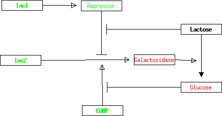
Figure 7: Lac operon after the modifications

Other parameters, such as the number of time steps, the number of modifications to make for graph updating, queries etc. are set via the command line.

8.2 Resolution engine

The resolution engine is able to perform the following reasoning tasks.

Graph validation.

This task consists in checking whether the graph ${\cal G}$ is consistent. The temporal encoding of ${\cal G}$ is grounded to the specified time and the SAT solver Picosat is used in a straightforward way in order to check the consistence of the grounded theory.

Graph querying.

This task consists in finding which initial values of the free atoms make ${\cal G}$ satisfy some temporal property $\varphi$. It is an abductive reasoning task [23], that could be solved by use of classical algorithms for computing prime implicants. But we have checked that, for instance, the Kean and Tsiknis algorithm [25] results to be very slow even when the total number of atoms is small. However, biologists are usually only interested by the values of the free atoms. Since their number is often quite small, it is usually faster to use Picosat to solve iteratively all possible models. In other terms, all the possible combinations of initial values for free atoms are generated (by the formula enumerator of figure 5) and the SAT solver is run on each of the so-obtained initial conditions. The system, tested on graphs with up to 22 nodes and 41 relations, showed to be effective up to roughly 16 to 20 free atoms depending on the complexity of the map.

In performing this task, exogenous and endogenous atoms can be treated differently: the user can either ask which values of all the free variables imply the given property, or else to find out which values of the free exognenous atoms guarantee that for all values of the free endogenous ones the query holds at the given time.

Graph updating.

Given a graph ${\cal G}$ for which a given property $\varphi$ does not hold, this task consists in turning ${\cal G}$ into a new graph ${\cal G^{\prime}}$ satisfying $\varphi$. This is the most complex task, since there is a very large number of possible graphs solving the problem. Currently, the system computes all graphs ${\cal G}^{\prime}$ that can be obtained from ${\cal G}$ by adding, removing or modifying a single relation (this step is called the graph enumerator in figure 5). Then for each ${\cal G}^{\prime}$, graph querying on ${\cal G}^{\prime}$ and $\varphi$ is performed, in order to filter out those which do not satisfy $\varphi$. .

9 Examples

The software tool has been tested on graphs with up to 20 atoms, 22 nodes and 41 links. In this section we show some examples of the two most complex tasks: graph querying and graph updating.

9.1 Graph querying

A more complex example will be considered here, i.e., a meaningful part of the map presented in Gigure 1, the atm-chk2 metabolic pathway, which leads to cellular apoptosis when the DNA double strand breaks. DNA double strand break (dsb) is a major cause of cancers, and medical and pharmaceutical research [26, 21] have shown that dsb can occur in a cell as the result of a pathology in a metabolic pathway. This kind of map is used to find the molecular determinants of tumoral response to cancers. Molecular parameters included the metabolic pathways for repairing DNA, the metabolic pathways for apoptosis, and the metabolic pathways of cellular cycle control [33, 26, 21, 28, 31]. When DNA is damaged, cellular cycle control points are activated and can quickly kill the cell by apoptosis, or stop the cellular cycle to enable DNA repair before reproduction of cellular division. Two of these control points are the metabolic pathways atm-chk2 and atr-chk2 [33].

The graph of Figure 8 (built from the map in Figure 1) represents the metabolic pathway atm-chk2 which can lead to apoptosis in three different ways. This map involves 20 variables, six of which (atm, dsb, chk2, mdm2, pml and p53) are exogenous and the rest endogenous. Some of these variables are proteins, others, such as dsb or apoptose, representing cell death, are conditions or states.

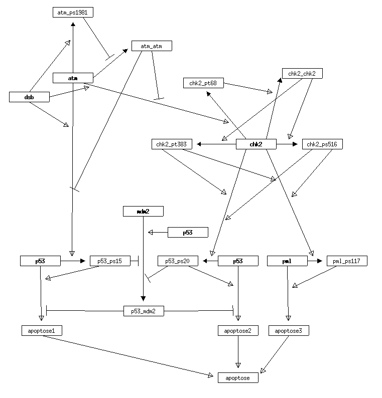
Figure 8: The Molecular Interaction Map atm-chk2

The time required for solving graph querying problems depends on the number of free variables and time steps. The P3M solver has been called on this graph to find out what would cause the cell apoptosis. It has been tested with different grounding values $g$, ranging from 1 to 50, and queries to find out the initial conditions that make the atom $apoptose(g)$ derivable, i.e., the conditions causing cell apoptosis at time $g$. The system has been tested with a number of free variables ranging from 6 (only exogenous variables are free) to 20 (all variables are set to free, thus asking the system to find also their initial values).

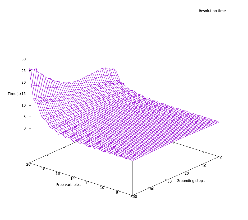
Figure 9: Time as a function of the number of grounding steps and free variables

The 3D diagram in Figure 9 plots the grounding values and the number of free variables against the time taken by the system to solve the problem, by calling Picosat (the time taken to encode the graph into propositional logic is negligible). From the diagram, it is clear that the number of free variables is the bottleneck, as it was actually expected since the time required to solve the problem is exponential in the number of free variables. Moreover, 50 time steps are overkill, most systems reaching a stable state in less than 10 time steps.

The questions asked to the system can be refined, in order to find out, for instance, how much time is required to reach apoptosis on each of the three possible ways, and which are the initial conditions which lead to each of them. The questions to ask are apoptose1(i), apoptose2(i) and apoptose3(i), for different values of $i$, where a query of the form $p(i)$ means that one looks for an explanation of $p$ being true at time step $i$. The answers given by the system show that:

• apoptose1 can be obtained is the in the fastest way: apoptose1(2) (apoptose1 holding at the second time step) is true if atm, dsb and p53 are present, and mdm2 is absent (the values of pml and chk2 do not matter). For $i\geq 3$, the answer to apoptose1(i) is the same, but mdm2 does not matter any longer (p53_mdm2 is dissociated at step 2).

• obtaining apoptose2 requires 5 time steps; atm, chk2, dsb, p53 have to be present, and mdm2 and pml do not matter.

• apoptose3 requires the same number of steps as apoptose2 but the initial conditions are different: atm, chk2, dsb, and pml have to be present, while mdm2 and p53 do not matter.

9.2 Graph updating

Figure 10 shows the map of the lac operon where the inhibition of lactose on the negative regulation of the repressor to the production of galactosidase has been suppressed. So here, glucose is not produced anymore when lactose is present.

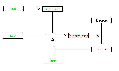
Figure 10: Lac operon without inhibition by lactose

The user can ask the system what modifications could be done in order to produce glucose when lactose is present. The “correct” solution is found immediately (Figure 11), along with others. Some of these other generated solutions have no interest, such as the direct production of glucose by genes lacZ or lacl. But the system also proposes reasonable solutions, such as that shown in Figure 12, where glucose is used to provide the inhibiting action for the repressor protein. When glucose is present, the production of galactosidase is stopped, while it is done when glucose is absent. However nature has chosen the more economical solution, because here galactosidase would be produced as soon as glucose is absent, which is useless if there is no lactose.

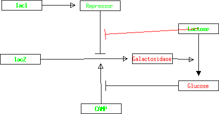
Figure 11: Correct solution

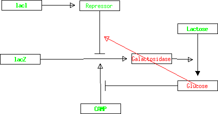
Figure 12: Another interesting solution

10 Conclusion

This paper presents a method to translate MIMs, representing biological systems, into Linear Temporal Logic, and a software tool able to solve complex questions on these graphs. The system, though still a prototype, is able to solve quite realistic examples of a large size.

The proposed approach can be improved in different directions. On the theoretical side, it is worth remarking that the speed of reactions is not taken into account. This limitation could be overcome by using the dual of speed (duration) and by using a logic that represents the duration of reactions. Moreover, the system relies on the “all or nothing” hypothesis: we do not represent quantities other than “absent” or “present”. As a consequence, all productions that are enabled at a given time are fired simultaneously, since they do not compete on the use of resources. Even if we have been able to efficiently model complex graphs with this constraint, an important step forward to be planned is modelling a more realistic evolution of networks by taking quantities into account.

On the practical point of view, the possibility should be explored to avoid grounding and replacing the formula enumerator procedure of P3M by implementing a direct abduction algorithm for (a suitable fragment of) LTL, as proposed in [9], or else by directly using temporal model checkers [13], or tools like RECAR (Recursive Explore and Check Abstraction Refinement ) [27] which allows one to solve modal satisfiability problems .

Moreover, the software tool can be improved in several respects like, for instance, improving the graphical interface by enriching the number of parameters the user can choose and making it more user friendly.

References

- [1] Jean-Marc Alliot, Robert Demolombe, Martín Diéguez, Luis Fariñas del Cerro, Gilles Favre, Jean-Charles Faye, Naji Obeid, and Olivier Sordet. Temporal logic modeling of biological systems. In Towards Paraconsistent Engineering, pages 205–226. Springer International Publishing, 2016.
- [2] Jean-Marc Alliot, Robert Demolombe, Luis Fariñas del Cerro, Martín Diéguez, and Naji Obeid. Abductive reasoning on molecular interaction maps. In Interactions Between Computational Intelligence and Mathematics, pages 43–56. Springer International Publishing, 2018.
- [3] Jean-Marc Alliot, Martín Diéguez, and Luis Fariñas del Cerro. Metabolic pathways as temporal logic programs. In Loizos Michael and Antonis Kakas, editors, Logics in Artificial Intelligence, pages 3–17. Springer International Publishing, 2016.
- [4] Grégory Batt, Delphine Ropers, Hidde de Jong, Johannes Geiselmann, Radu Mateescu, Michel Page, and Dominique Schneider. Validation of qualitative models of genetic regulatory networks by model checking: analysis of the nutritional stress response in Escherichia coli. In Proceedings Thirteenth International Conference on Intelligent Systems for Molecular Biology 2005, Detroit, MI, USA, 25-29 June 2005, pages 19–28, 2005.
- [5] Armin Biere. Picosat essentials. Journal on Satisfiability, Boolean Modeling and Computation (JSAT), 4:75–97, 2008.
- [6] D. Bošnački, P.A.J. Hilbers, R.S. Mans, and E.P. de Vink. Chapter 39: Modeling and analysis of biological networks with model checking. In M. Elloumi and A.Y. Zomaya, editors, Algorithms in Computational Molecular Biology: Techniques, Approaches and Applications, volume 1 of Wiley Series in Bioinformatics, pages 915–940. Wiley, 2011.
- [7] Luboš Brim, Milan Češka, and David Šafránek. Model Checking of Biological Systems. In Formal Methods for Dynamical Systems: 13th International School on Formal Methods for the Design of Computer, Communication, and Software Systems, SFM 2013, Bertinoro, Italy, June 17-22, 2013. Advanced Lectures, pages 63–112. Springer Berlin Heidelberg, Berlin, Heidelberg, 2013.
- [8] Laurence Calzone, François Fages, and Sylvain Soliman. BIOCHAM: an environment for modeling biological systems and formalizing experimental knowledge. Bioinformatics, 22(14):1805–1807, 2006.
- [9] Serenella Cerrito, Marta Cialdea Mayer, and Robert Demolombe. Temporal abductive reasoning about biochemical reactions. Journal of Applied Non-Classical Logics, 27(3-4):269–291, 2017.
- [10] Nathalie Chabrier-Rivier, Marc Chiaverini, Vincent Danos, François Fages, and Vincent Schächter. Modeling and querying biomolecular interaction networks. Theoretical Computer Science, 325(1):25–44, 2004.
- [11] Nathalie Chabrier-Rivier, Francois Fages, and Sylvain Soliman. The Biochemical Abstract Machine BIOCHAM. In Vincent Danos and Vincent Schächter, editors, CMSB’04: Proceedings of the second Workshop on Computational Methods in Systems Biology, volume 3082, pages 172–191, Paris, 2004. Springer-Verlag.
- [12] Federica Ciocchetta and Jane Hillston. Bio-pepa: An extension of the process algebra pepa for biochemical networks. Electron. Notes Theor. Comput. Sci., 194(3):103–117, 2008.
- [13] Edmund Clarke, Orna Grumberg, Somesh Jha, Yuan Lu, and Helmut Veith. Counterexample-guided abstraction refinement for symbolic model checking. Journal of the ACM, 50(5):752–794, 2003.
- [14] R. Demolombe, L. Fariñas del Cerro, and N. Obeid. Automated reasoning in metabolic networks with inhibition. In 13th International Conference of the Italian Association for Artificial Intelligence, (AI*IA’13), pages 37–47, Turin, Italy, 2013.
- [15] R. Demolombe, L. Fariñas del Cerro, and N. Obeid. Translation of first order formulas into ground formulas via a completion theory. Journal of Applied Logic, 15:130–149, 2016.
- [16] Robert Demolombe, Luis Fariñas del Cerro, and Naji Obeid. A logical model for molecular interaction maps. In Fariñas and Inoue [19], chapter 3, pages 93–123.
- [17] Francois Fages and Sylvain Soliman. Formal Cell Biology in Biocham. In Formal Methods for Computational Systems Biology: 8th International School on Formal Methods for the Design of Computer, Communication, and Software Systems, SFM 2008 Bertinoro, Italy, June 2-7, 2008 Advanced Lectures, pages 54–80. Springer Verlag, Berlin, Heidelberg, 2008.
- [18] Francois Fages, Sylvain Soliman, and Nathalie Chabrier-rivier. Modelling and querying interaction networks in the biochemical abstract machine biocham. Journal of Biological Physics and Chemistry, 4:64–73, 2004.
- [19] L. Fariñas and K. Inoue, editors. Logical Modeling of Biological Systems. John Wiley & Sons, 2014.
- [20] Fisher Jasmin and Henzinger Thomas A. Executable cell biology. Nat Biotech, 25(11):1239–1249, nov 2007.
- [21] V. Glorian, G. Maillot, S. Poles, J. S. Iacovoni, G. Favre, and S. Vagner. HuR-dependent loading of miRNA RISC to the mRNA encoding the Ras-related small GTPase RhoB controls its translation during UV-induced apoptosis. CCell Death and Differentiation, 18(11):1692–1701, 2011.
- [22] M. Hucka, H. Bolouri, A. Finney, H. M. Sauro, J. C. Doyle, and H. Kitano. The systems biology markup language (SBML): A medium for representation and exchange of biochemical network models. Bioinformatics, 19:524–531, 2003.
- [23] Katsumi Inoue. Linear resolution for consequence finding. Artificial Intelligence, 56(2):301 – 353, 1992.
- [24] F. Jacob and J. Monod. Genetic regulatory mechanisms in the synthesis of proteins. Journal of Molecular Biology, 3:318–356, 1961.
- [25] A. Kean and G. Tsiknis. An incremental method for generating prime implicants/implicates. Journal of Symbolic Computing, 9:185–206, 1990.
- [26] K. W. Kohn and Y. Pommier. Molecular interaction map of the p53 and Mdm2 logic elements, which control the off-on swith of p53 response to DNA damage. Biochemical and Biophysical Research Communications, 331(3):816–827, 2005.
- [27] Jean-Marie Lagniez, Daniel Le Berre, Tiago de Lima, and Valentin Montmirail. A recursive shortcut for CEGAR: Application to the modal logic K satisfiability problem. In Proceedings of the Twenty-Sixth International Joint Conference on Artificial Intelligence (IJCAI-17), pages 674–680, 2017.
- [28] W. J. Lee, D. U. Kim, M. Y. Lee, and K. Y. Choi. Identification of proteins interacting with the catalytic subunit of PP2A by proteomics. Proteomics, 7(2):206–214, 2007.
- [29] Xavier Leroy, Damien Doligez, Alain Frisch, Jacques Garrigue, Didier Rémy, and Jérôme Vouillon. The OCaml System, Documentation and user’s manual. Institut National de Recherche en Informatique et en Automatique, 2017.
- [30] Alida Palmisano and Corrado Priami. Bio-PEPA. In Encyclopedia of Systems Biology, pages 145–146. Springer New York, New York, NY, 2013.
- [31] H. Pei, L. Zhang, K. Luo, Y Qin, M. Chesi, F Fei, P. L. Bergsagel, Wang L., Z. You, and Z. Lou. MMSET regulates histone H4K20 methylation and 53BP1 accumulation at DNA damage sites. Nature, 470(7332):124–128, 2011.
- [32] A. Pnueli. The temporal logic of programs. In Proc. of the 18th Annual Symposium on Foundations of Computer Science, pages 46–57, Providence, Rhode Island, USA, 1977.
- [33] Y. Pommier, O. Sordet, V. A. Rao, H. Zhang, and K.W. Kohn. Targeting chk2 kinase: molecular interaction maps and therapeutic rationale. Current Pharmaceutical Design, 11(22):2855–2872, 2005.
- [34] Raymond Reiter. Knowledge in Action: Logical Foundations for Specifying and Implementing Dynamical Systems. MIT Press, 2001.
- [35] Mara Sangiovanni. Model Checking of Metabolic Networks: Application to Metabolic Diseases. PhD thesis, Federico II University of Naples., 2014.
- [36] Jetse Scholma, Stefano Schivo, Ricardo A. Urquidi Camacho, Jaco van de Pol, Marcel Karperien, and Janine N. Post. Biological networks 101: Computational modeling for molecular biologists. Gene, 533(1):379–384, 2014.
- [37] Wikipedia. The lac operon. https://en.wikipedia.org/wiki/Lac\_operon, 2015.