BPS Maxwell-Chern-Simons vortices with internal structures: the Abelian Higgs and the gauged $CP(2)$ cases

Abstract

We investigate the existence of first-order vortices inherent to both the Maxwell-Chern-Simons-Higgs and the Maxwell-Chern-Simons-$CP(2)$ models extended via the inclusion of an extra scalar sector which plays the role of a source field. For both cases, we focus our attention on the time-independent configurations with radial symmetry which can be obtained through the implementation of the so-called Bogomol’nyi-Prasad-Sommerfield (BPS) prescription. In this sense, in order to solve the corresponding first-order differential equations, we introduce some particular scenarios which are driven by the source field whose presence, we expect, must change the way the resulting vortices behave. After solving the effective first-order system through a finite-difference algorithm, we comment about the main new effects induced by the presence of the source field in the shape of the final configurations.

I Introduction

In the context of classical field theories, the configurations with nontrivial topology are solutions of highly nonlinear second-order field equations driven by the presence of a symmetry-breaking potential n5 which characterizes a phase transition. However, under exceptional circumstances, they can also be studied as the solutions of a set of coupled first-order differential equations obtained from the minimization of the effective energy functional through the Bogomolnyi-Prasad-Sommerfield (BPS) formalism n4 . Other methods which also lead to the first-order equations include the study of the conservation of the energy-momentum tensor ano and the so-called On-Shell Method onshell . In this scenario, first-order vortices were obtained not only in the Maxwell-Higgs model n1 but also in the Chern-Simons-Higgs cshv and in the Maxwell-Chern-Simons-Higgs mcshv ones.

More recently, based on the exploration of the phenomenological relation between the gauged $CP(N)$ and the 4D Yang-Mills models, Loginov loginov has shown the existence of vortex solutions in a Maxwell-$CP(2)$ model. By following such an approach, some of us have obtained first-order vortices in a Maxwell-$CP(2)$ casana , in a Chern-Simons-$CP(2)$ vini and also in a Maxwell-Chern-Simons-$CP(2)$ neyver theories.

Another interesting issue is the existence of first-order vortices in the context of enlarged gauged models. In this context, it is worthwhile to highlight that the usual Maxwell-Higgs model itself was extended to accommodate an $SO(3)$ group by the inclusion of an extra scalar sector witten . In addition, a recent work n44 has verified that such enlarged theory indeed supports first-order vortices with internal structures, which may find relevant applications in the context of metamaterials n45 . Besides this point, the existence of such vortices was also shown to occur in an extended Maxwell-$CP(2)$ model joao .

The manuscript aims to go further by investigating whether first-order vortices with internal structures can be obtained in both Maxwell-Chern-Simons-Higgs and Maxwell-Chern-Simons-$CP(2)$ when enlarged to include an extra real scalar field.

We have organized our results as follows: In Sec. II, we define an extended Maxwell-Chern-Simons-Higgs (MCSH) model via the inclusion of a real scalar field (i.e., the source field $\chi$). Besides, the extended model also contains two arbitrary functions: the superpotential $W(\chi)$ characterizing the vacuum manifold related to the source field, and a dielectric function $G(\chi)$ multiplying the Maxwell term. We focus the attention in those time-independent configurations possessing radial symmetry obtained via the Bogomol’nyi-Prasad-Sommerfield (BPS) algorithm. The technique provides the Bogomol’nyi bound for the total energy and the first-order differential equations themselves. The simplified structure of the BPS equation for the source field allows us to obtain the solution by fixing the superpotential $W$. In the sequence, we solve the remaining two BPS equations and the Gauss law through a finite-difference scheme for two different choices of the dielectric function $G$. Further, we depict the numerical results for the relevant fields and identify the internal structure caused by the presence of the source field. In the Sec. III, we study an extended Maxwell-Chern-Simons-$CP(2)$ (MCS-$CP(2)$) model within the context presented in the previous section but more complicated from the technical point-of-view. In both extended models, the solutions share similar effects produced by the dielectric function. We end our manuscript in Sec. IV, in which we summarize our results and enunciate our perspectives regarding future investigations.

In what follows, we use $\eta^{\mu\nu}=(+--)$ as the metric signature of the (2+1)-dimensional flat spacetime, together with the natural units system, for simplicity.

II The Maxwell-Chern-Simons-Higgs case

In this Section, we begin the investigation about the existence of first-order vortices with internal structures in an extended Maxwell-Chern-Simons-Higgs scenario. Here, it is worthwhile to emphasize some useful observations. The first one is that in typical MCSH scenario, the correct implementation of the BPS prescription is known to be possible only when the original model is enlarged via the inclusion of a neutral scalar field $\Psi$ mcshv . Second, the occurrence of the internal structures depends on the presence of an additional real scalar field $\chi$ (the so-called source field) n44 .

Therefore, based on the positive results concerning the insertion of internal structures in the Maxwell-Higgs n44 and in the Maxwell-$CP(2)$ joao models, we propose as our starting-point the following Lagrangian density in order to study vortices with internal structure in a Maxwell-Chern-Simons-Higgs scenario (here, $\kappa$ and $e$ are the usual coupling constants, while $v$ stands for the vacuum expectation value for the complex Higgs field),

$$\mathcal{L} = -\frac{G(\chi)}{4}F_{\mu\nu}F^{\mu\nu}-\frac{\kappa}{4}\epsilon^{\mu\nu\kappa}A_{\mu}F_{\nu\kappa}+D^{\mu}\phi\overline{D_{\mu}\phi}$$ (1)

$$+\frac{G(\chi)}{2}\partial_{\mu}\Psi\partial^{\mu}\Psi+\frac{1}{2}\partial_{\mu}\chi\partial^{\mu}\chi-U\left(\left|\phi\right|,\Psi,\chi\right)\text{,}$$

where $A_{\mu}$ is the electromagnetic field, $F_{\mu\nu}=\partial_{\mu}A_{\nu}-\partial_{\nu}A_{\mu}$ represents its strength tensor and $\epsilon^{\mu\nu\kappa}$ is the Levi-Civita tensor (with $\epsilon^{012}=+1$). The coupling between the electromagnetic and Higgs fields is accounted by the standard covariant derivative,

$$D_{\mu}\phi=\partial_{\mu}\phi-ieA_{\mu}\phi\text{.}$$ (2)

We also point out the presence of a dielectric function $G\equiv G(\chi)$ multiplying both the Maxwell and the kinetic term for the field $\Psi$. As we demonstrate below, such a function is the responsible for the formation of the internal structure inherent to the vortex configurations.

In the present case, we choose the potential as

$$U(|\phi|,\Psi,\chi) = \frac{1}{2G}\left[e\left(v^{2}-\left|\phi\right|^{2}\right)-\kappa\Psi\right]^{2}$$ (3)

$$+e^{2}\left|\phi\right|^{2}\Psi^{2}+\frac{1}{2r^{2}}\left(\frac{dW}{d\chi}\right)^{2}\text{,}$$

where the first two terms in the right-hand side (with $G=1$) correspond to the potential which allows the standard Maxwell-Chern-Simons-Higgs model to be self-dual mcshv . In our enlarged case, the third term stands for the potential related to the source field, with $W=W(\chi)$ being called superpotential. Here, even though the breaking of the translational invariance (from which we conclude that the resulting model must be seen therefore as an effective one), the factor $1/r^{2}$ is included to support the obtainment of the first-order equation for the source field itself n44 .

The presence of the Chern-Simons term does not allow the implementation of the gauge choice $A_{0}=0$ given that this choice does not solve the corresponding Gauss law, from which we conclude that the resulting structures possess nontrivial profiles for both the electric and the magnetic fields. Consequently, it is reasonable to expect that the internal structure will be present in both the electric and the magnetic sectors.

We look for time-independent configurations via the standard radially symmetric map which is given by (the Latin indexes run over the spatial coordinates only)

$$\phi=vg(r)e^{in\theta}\text{ \ and \ }A_{i}=\varepsilon_{ij}\frac{x_{j}}{er^{2}}\left[a(r)-n\right]\text{,}$$ (4)

where $r$ and $\theta$ are the polar coordinates, $\varepsilon_{ij}$ stands for the antisymmetric symbol, $x_{j}$ is the unit vector and the integer parameter $n=\pm 1,$ $\pm 2,$ $\pm 3...$ represents the winding number (vorticity) of the final solutions. In view of this map, we also get that $A_{0}=A_{0}(r)$, $\Psi=\Psi(r)$ and $\chi=\chi(r)$. Moreover, the dimensionless profile functions $g(r)$ and $a(r)$ are supposed to behave as

$$g(r=0)=0\text{ \ and \ }a(r=0)=n\text{,}$$ (5)

$$g(r\rightarrow\infty)\rightarrow 1\text{ \ and \ }a(r\rightarrow\infty)\rightarrow 0\text{,}$$ (6)

from which we expect to obtain regular solutions with finite energy.

We focus our attention on those vortex solutions satisfying a particular set of coupled first-order differential equations. These equations arise through the implementation of the BPS prescription (i.e. the minimization of the energy of the model (1)). The starting-point is the radially symmetric expression for the stationary energy distribution given by

$$\varepsilon = \frac{G}{2}B^{2}+\frac{G}{2}\left(\frac{dA_{0}}{dr}\right)^{2}+v^{2}\left(\left(\frac{dg}{dr}\right)^{2}+\frac{a^{2}g^{2}}{r^{2}}\right)$$ (7)

$$+e^{2}v^{2}g^{2}\left(A_{0}\right)^{2}+\frac{G}{2}\left(\frac{d\Psi}{dr}\right)^{2}+\frac{1}{2}\left(\frac{d\chi}{dr}\right)^{2}$$

$$+\frac{1}{2G}\left[ev^{2}\left(1-g^{2}\right)-\kappa\Psi\right]^{2}$$

$$+e^{2}v^{2}g^{2}\Psi^{2}+\frac{1}{2r^{2}}\left(\frac{dW}{d\chi}\right)^{2}\text{,}$$

which, after some algebraic manipulation, can be promptly rearranged as

$$\varepsilon = \varepsilon_{{BPS}}+\frac{1}{2G}\left(\frac{{}}{{}}GB\mp\left[ev^{2}\left(1-g^{2}\right)-\kappa\Psi\right]\right)^{2}$$ (8)

$$+v^{2}\left(\frac{dg}{dr}\mp\frac{ag}{r}\right)^{2}+\frac{1}{2}\left(\frac{d\chi}{dr}\mp\frac{1}{r}\frac{dW}{d\chi}\right)^{2}$$

$$+\frac{1}{2}G\left(\frac{dA_{0}}{dr}\mp\frac{d\Psi}{dr}\right)^{2}+e^{2}v^{2}g^{2}\left(A_{0}\mp\Psi\right)^{2}\text{,}$$

where we have defined the term $\varepsilon_{{BPS}}$ as

$$\varepsilon_{{BPS}}=\mp\frac{v^{2}}{r}\frac{d}{dr}\left[a\left(1-g^{2}\right)\right]\pm\frac{1}{r}\frac{dW}{dr}\text{,}$$ (9)

whose integration over the plane, using the boundary conditions (5) and (6), provides the expression which becomes the Bogomol’nyi bound for the extended MCSH model, i.e.

$$E_{BPS}=2\pi\int_{0}^{\infty}r\varepsilon_{{BPS}}dr=\pm 2\pi\left(v^{2}n+\Delta W\right)\text{,}$$ (10)

with $\Delta W=W\left(r\rightarrow\infty\right)-W(r=0)$. In the expression above, the upper (lower) sign holds for positive (negative) values of both $n$ and $\Delta W$.

Considering these results, one gets that the total energy of the model satisfies

$$\left.\frac{E}{2\pi}=\int_{0}^{\infty}\frac{1}{2G}\left(\frac{{}}{{}}GB\mp\left[ev^{2}\left(1-g^{2}\right)-\kappa\Psi\right]\right)^{2}rdr\right.$$

$$\left.+\int_{0}^{\infty}\left[v^{2}\left(\frac{dg}{dr}\mp\frac{ag}{r}\right)^{2}+\frac{1}{2}\left(\frac{d\chi}{dr}\mp\frac{1}{r}\frac{dW}{d\chi}\right)^{2}\right]rdr\right.$$

$$\left.+\int_{0}^{\infty}\left[\frac{G}{2}\left(\frac{dA_{0}}{dr}\mp\frac{d\Psi}{dr}\right)^{2}+e^{2}v^{2}g^{2}\left(A_{0}\mp\Psi\right)^{2}\right]rdr\right.$$

$$\left.+\frac{E_{BPS}}{2\pi}\geq v^{2}\left|n\right|+\left|\Delta W\right|\text{,}\right.$$ (11)

which reveals that the energy is indeed bounded from below and that the bound is saturated when the fields satisfy

$$GB=\pm ev^{2}\left(1-g^{2}\right)\mp\kappa\Psi\text{,}$$ (12)

$$\frac{dg}{dr}=\pm\frac{ag}{r}\text{,}$$ (13)

$$\frac{d\chi}{dr}=\pm\frac{1}{r}\frac{dW}{d\chi}\text{,}$$ (14)

$$\frac{d\Psi}{dr}=\pm\frac{dA_{0}}{dr}\text{ \ and \ }\Psi=\pm A_{0}\text{.}$$ (15)

Therefore, the system above stands for the first-order BPS equations of the model (also here, the upper (lower) sign holds for $n>0$ ($n<0$)). In particular, when these first-order equations are satisfied, the energy of the resulting BPS configurations is equal to $E_{BPS}$, the corresponding Bogomol’nyi bound, calculated in (10).

In view of the Eq. (15), we point out that $\Psi=\pm A_{0}$ also solves the $\Psi^{\prime}=\pm A_{0}^{\prime}$ (here, prime denotes the derivative with respect to the radial coordinate). As usual, the solution for the scalar potential $A_{0}(r)$ is obtained by solving the Gauss law which, given the radially symmetric scenario, takes the form

$$\frac{1}{r}\frac{d}{dr}\left(rG\frac{dA_{0}}{dr}\right)+\kappa B=2e^{2}v^{2}g^{2}A_{0}\text{.}$$ (16)

It must be solved (together with the remaining three first-order equations above) according to the boundary conditions

$$A_{0}(r=0)=w_{0}\text{ \ and \ }A_{0}^{\prime}(r\rightarrow\infty)\rightarrow 0\text{,}$$ (17)

where $w_{0}=A_{0}(0)$ stands for a constant.

II.1 Some MCSH scenarios with internal structure

We now proceed with the construction of some particular scenarios and their respective numerical solutions. We begin this task by pointing out that the first-order equation for the source field $\chi$ does not contain the other fields of the model and depends only on the form of the superpotential $W(\chi)$. Here, we choose the superpotential as

$$W(\chi)=\chi-\frac{1}{3}\chi^{3}\text{,}$$ (18)

which was used recently as an attempt to understand planar skyrmion-like solitons 2324 and the behavior of massless Dirac fermions in a skyrmion-like background 25 .

In view of this choice, the first-order equation (14) for the source field can be written in the form

$$\frac{d\chi}{dr}=\pm\frac{1}{r}\left(1-\chi^{2}\right)\text{,}$$ (19)

whose exact solution reads

$$\chi(r)=\pm\frac{r^{2}-r_{0}^{2}}{r^{2}+r_{0}^{2}}\text{,}$$ (20)

where $r_{0}$ represents an arbitrary positive constant such that $\chi\left(r=r_{0}\right)=0$. We note that this solution attains the boundary values $\chi\left(r=0\right)=\mp 1$ and $\chi\left(r\rightarrow\infty\right)\rightarrow\pm 1$.

We also rewrite the BPS energy density (9) as

$$\varepsilon_{BPS}=\varepsilon_{G}+\varepsilon_{\chi}\text{,}$$ (21)

where $\varepsilon_{G}$ represents the contribution which refers to the vortex with internal structure, i.e.

$$\varepsilon_{G}=G\left[B^{2}+\left(\frac{dA_{0}}{dr}\right)^{2}\right]+2v^{2}\left[e^{2}g^{2}\left(A_{0}\right)^{2}+\frac{a^{2}g^{2}}{r^{2}}\right]\text{,}$$ (22)

while $\varepsilon_{\chi}$ corresponds to the contribution related exclusively to the source field $\chi$, i.e.

$$\varepsilon_{\chi}=\left(\frac{d\chi}{dr}\right)^{2}\text{.}$$ (23)

In order to proceed with our investigation, we now need to choose a particular expression for the dielectric function $G(\chi)$. In this regard, for pedagogical reasons, we separate our study in two different scenarios.

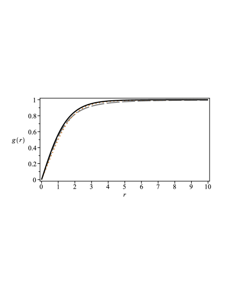
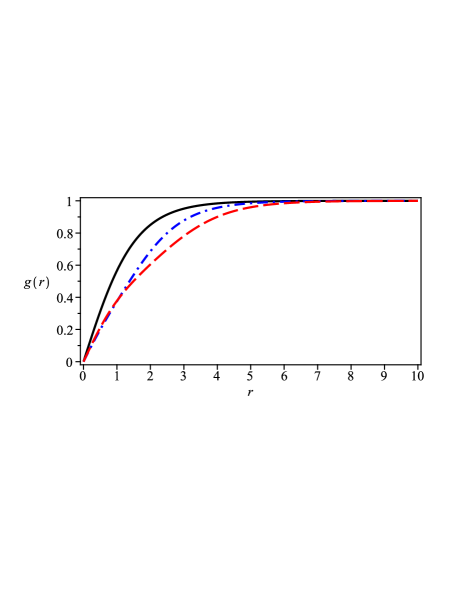
Figure 1: Numerical solutions to the scalar profile function $g\left(r\right)$ coming from (26), (27) and (28) (top, long-dashed gray line for $r_{0}=1$ and dotted orange line for $r_{0}=2$) and (40), (41) and (42) (bottom, dash-dotted blue line for $r_{0}=1$ and dashed red line for $r_{0}=2$). In both cases, the equations were solved according the boundary conditions (5), (6) and (17). We have used $e=v=\kappa=1$ and $n=1$ (i.e. upper signs in the first-order expressions). Here, the solid black line is the usual solution (absence of the source field, with $G=1$).

II.1.1 The first case

In what follows, we choose the dielectric function as

$$G(\chi)=\frac{1}{1-\chi^{2}}\text{,}$$ (24)

which, taking into account the solution (20), can be expressed as

$$G(r)=\frac{\left(r^{2}+r_{0}^{2}\right)^{2}}{4r^{2}r_{0}^{2}}\text{,}$$ (25)

which is finite along the radial axis but diverges at the boundaries (i.e. for $r=0$ and $r\rightarrow\infty$), see the Eq. (20). Therefore, in order to avoid that the first two terms in the right-hand side of the Eq. (7) to be singular, the magnetic and electric fields must vanish at the boundaries, from which the total energy is expected to converge to the finite value given by (10).

By using (25), the first-order equations (12) and (13) assume the form

$$\frac{1}{r}\frac{da}{dr}=\frac{4r^{2}r_{0}^{2}}{\left(r^{2}+r_{0}^{2}\right)^{2}}\left(\mp e^{2}v^{2}\left(1-g^{2}\right)+e\kappa A_{0}\right)\text{,}$$ (26)

$$\frac{dg}{dr}=\pm\frac{ag}{r}\text{,}$$ (27)

while the Gauss law can be written as

$$\frac{1}{4r_{0}^{2}r}\frac{d}{dr}\left[\frac{\left(r^{2}+r_{0}^{2}\right)^{2}}{r}\frac{dA_{0}}{dr}\right]+\kappa B=2e^{2}v^{2}g^{2}A_{0}\text{,}$$ (28)

where we have used

$$B(r)=-\frac{1}{er}\frac{da}{dr}\text{,}$$ (29)

which stands for the radially symmetric expression for the magnetic field.

Hereinafter, we fix the constants of the model as $e=v=\kappa=1$ and $n=1$ (i.e. upper signs in the first-order expressions), from which we solve the equations (26), (27) and (28) above for $r_{0}=1$ (long-dashed gray line) and $r_{0}=2$ (dotted orange line) via the implementation of a finite-difference algorithm according the boundary conditions (5), (6) and (17). We then depict the numerical solutions for the profile functions $g(r)$ and $a(r)$, the electric potential $A_{0}(r)$, the magnetic $B(r)$ and electric $E(r)$ fields, and the energy distribution $\varepsilon_{BPS}$, see the figures 1-6 below (in which the solid black line represents the usual solution).

Figures 1 and 2 show the Higgs profile $g(r)$ and the gauge one $a(r)$, respectively. We see that, despite the presence of the source field, these functions converge naturally to the boundary values given by (5) and (6). In the present case, the effects caused by the source field are slight variations on the core-size of the corresponding solutions.

The solutions for the electric potential $A_{0}(r)$, depicted in the Fig. 3, show that the variation of $r_{0}$ changes both the core-size and the maximum value reached on the origin.

Figures 4 and 5 present, respectively, the profiles for the magnetic and electric fields, which stand for ring structures. In particular, we note that the magnetic field behavior is dramatically different from the usual one. As we have explained previously, in order to avoid the first two terms on the right-hand side of (7) to be singular, these fields vanish in the boundaries $r=0$ and $r\rightarrow\infty$, and this fact allows the the total energy to converge to the Bogomol’nyi bound (10). Furthermore, the variations on $r_{0}$ also affect both the core-size and the maximum value these solutions reach.

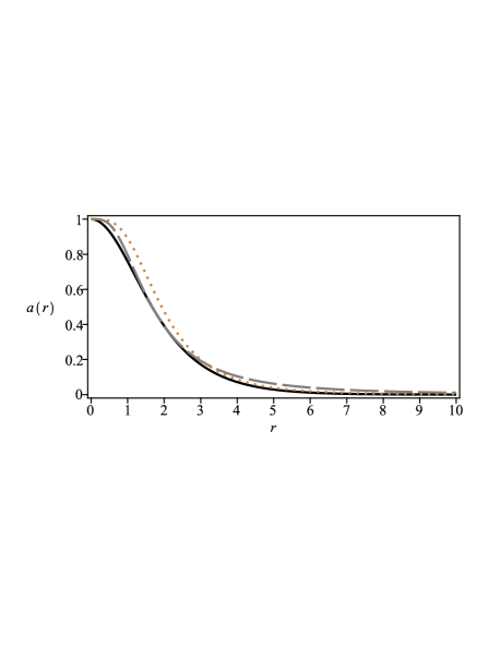
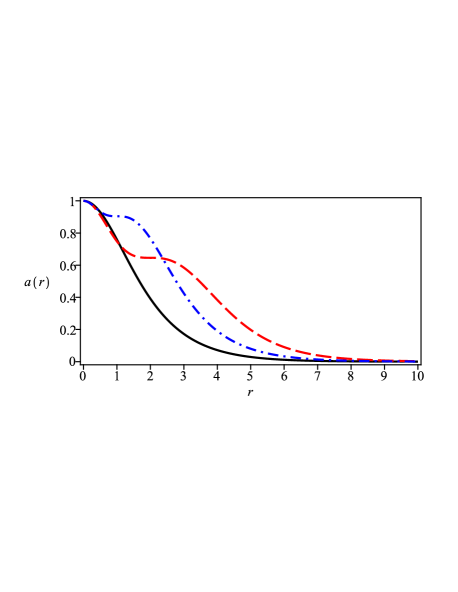
Figure 2: Numerical solutions to the gauge profile function $a(r)$. Conventions as in the Fig. 1. The solutions for the 1st. case mimic the usual ones around the point $r=r_{0}$, while the profiles for the 2nd. case have a plateau at $r=r_{0}$.

Finally, the profiles for the energy distribution $\varepsilon_{G}$ related to the BPS configurations are depicted in the Fig. 6, from which we see how the source field changes the shape of these solutions from a lump (standard profile) to a ring (nonusual ones), with $r_{0}$ also controlling the ”radius” (i.e. the distance from the origin for which the solution reaches its maximum value) of these rings.

Now, before studying a new case, it is interesting to investigate how the dielectric medium affects the way the fundamental fields behave close to the boundary values. With this purpose in mind, we solve the equations (26), (27) and (28) around the boundaries. In this case, for $n=N>0$, we get that, near the origin, the fields behave approximately as

$$g(r)\approx g_{N}r^{N}-\frac{eB_{0}}{4r_{0}^{2}}g_{N}r^{N+4}\text{,}$$ (30)

$$a(r)\approx N-\frac{eB_{0}}{r_{0}^{2}}r^{4}\text{,}$$ (31)

$$A_{0}(r)\approx w_{0}+w_{2}r^{2}-\frac{w_{2}}{r_{0}^{2}}r^{4}\text{,}$$ (32)

while the solutions in the limit $r\rightarrow\infty$ read

$$g(r)\approx 1-C_{\infty}r^{-\Lambda}\text{,}$$ (33)

$$a(r)\approx\Lambda C_{\infty}r^{-\Lambda}\text{,}$$ (34)

$$A_{0}(r)\approx-\frac{\Lambda C_{\infty}}{2e\kappa\left(r_{0}\right)^{2}}r^{-\Lambda}\text{,}$$ (35)

where $g_{N}>0$, $C_{\infty}>0$ and $w_{2}$ are positive integration constants. We have also defined

$$B_{0}=B\left(r=0\right)=v^{2}e-w_{0}\kappa\text{,}$$ (36)

i.e. the value of the magnetic field at the origin without the influence of the dielectric medium. Moreover, we have also introduced the parameter $\Lambda$ as

$$\Lambda=1+\sqrt{1+8\left(evr_{0}\right)^{2}}\text{,}$$ (37)

which shows how the dielectric medium (via $r_{0}$) controls the way the fields decay when $r\rightarrow\infty$.

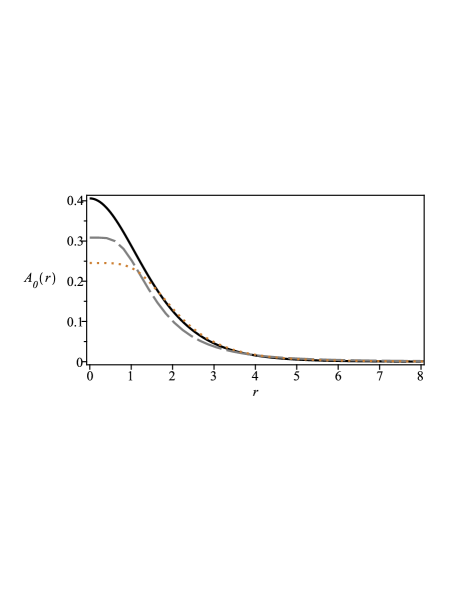
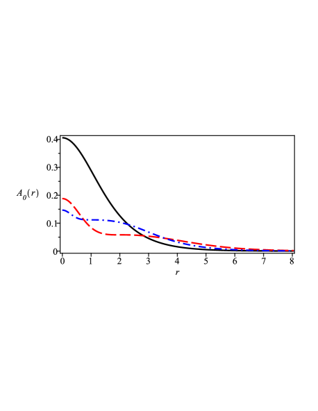
Figure 3: Numerical solutions to the electric potential $A_{0}(r)$. Conventions as in the Fig. 1. The solutions for the 1st. case mimic the standard behavior around $r=r_{0}$. The results for the 2nd. case also have a plateau at $r=r_{0}$.

II.1.2 The second case

We now consider another interesting choice for the dielectric function $G(\chi)$, whose expression reads

$$G(\chi)=\frac{1}{\chi^{2}}\text{,}$$ (38)

which behaves as $G(r=0)=1$ and $G(r\rightarrow\infty)\rightarrow 1$ when the field $\chi$ given by the Eq.(20). Consequently, at the boundaries, the new vortex configurations mimic the behavior of those obtained in the absence of the source field.

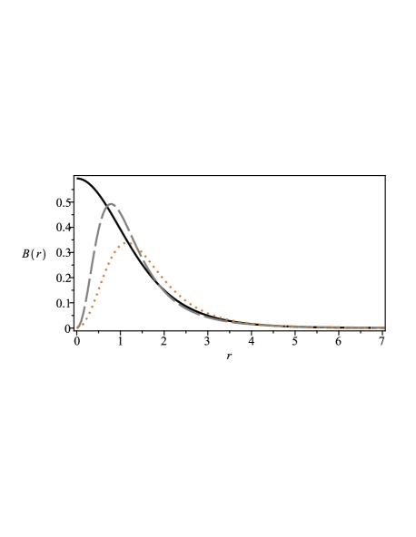
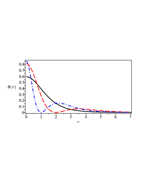
Figure 4: Numerical solutions to the magnetic field $B(r)$. Conventions as in the Fig. 1. The solutions for the 2nd. case vanish at $r=r_{0}$ (what can be understood as an internal structure) in order to avoid the first term in the right-hand side of the Eq. (7) to be singular.

Moreover, it is interesting to highlight that, when $r=r_{0}$, the source field $\chi$ given by (20) vanishes and that therefore the function $G$ in (38) diverges. This singularity is counterbalanced by the electric and magnetic fields, which must vanish $r=r_{0}$. This fact leads to a finite energy density (7) whose correspondent BPS total energy converges to the value (10). The vanishing of the electric and magnetic fields in $r=r_{0}$ is the manifestation of an internal structure in the vortex configurations.

We now use the Eq. (20) in order to rewrite the dielectric function given by (38) in the form

$$G(r)=\frac{\left(r^{2}+r_{0}^{2}\right)^{2}}{\left(r^{2}-r_{0}^{2}\right)^{2}}\text{,}$$ (39)

which leads to the first-order equations

$$\frac{1}{r}\frac{da}{dr}=\frac{\left(r^{2}-r_{0}^{2}\right)^{2}}{\left(r^{2}+r_{0}^{2}\right)^{2}}\left(\mp e^{2}v^{2}\left(1-g^{2}\right)+e\kappa A_{0}\right)\text{,}$$ (40)

$$\frac{dg}{dr}=\pm\frac{ag}{r}\text{,}$$ (41)

and to the Gauss law

$$\frac{1}{r}\frac{d}{dr}\left[\frac{\left(r^{2}+r_{0}^{2}\right)^{2}r}{\left(r^{2}-r_{0}^{2}\right)^{2}}\frac{dA_{0}}{dr}\right]+\kappa B=2e^{2}v^{2}g^{2}A_{0}\text{,}$$ (42)

where we have again used the Eq. (29) for the magnetic field.

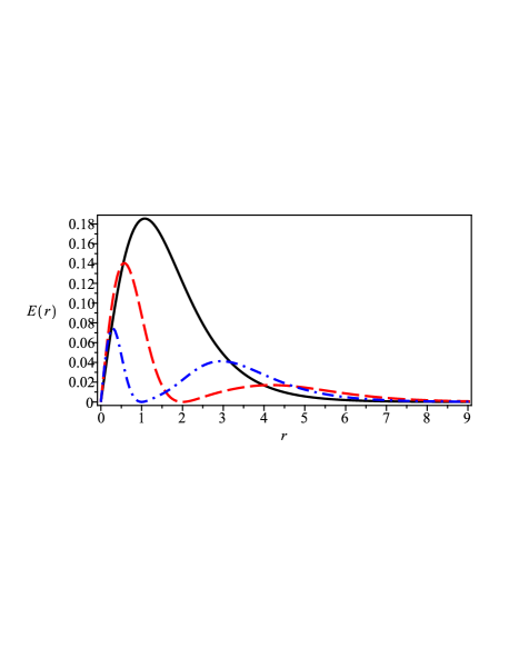
Figure 5: Numerical solutions to the electric field $E(r)$. Conventions as in the Fig. 1. The solutions for the 2nd. case vanish at $r=r_{0}$ (internal structure) in order to avoid the second term in the right-hand side of the Eq. (7) to be singular.

We now proceed with the numerical study of the equations (40), (41) and (42) according the boundary values (5), (6) and (17). Here, we again choose $e=v=\kappa=n=1$, from which we solve the equations for $r_{0}=1$ and $r_{0}=2$, see the dash-dotted blue and the dashed red lines, respectively. Furthermore, with the aim to compare the new results with the previous ones, we plot them in the same figures 1-6.

The profiles for the functions $g(r)$ and $a(r)$ naturally converge to the boundary values (5) and (6), see the figures 1 and 2. The novelty here is that the solutions for $a(r)$ now have a plateau at the point $r=r_{0}$. Here, it is worthwhile to note that the plateau at $r=r_{0}$ also occurs in the solutions for the electric potential $A_{0}(r)$, see Figure 3. As we explain below, these plateaus give rise to the emergence of the internal structure in the profiles for the magnetic and electric fields.

In the figures 4 and 5, one finds the numerical profiles for the magnetic and electric fields, respectively. In this case, we highlight the existence of internal structures for intermediate values of the radial coordinate $r$ (in particular, the corresponding fields vanish at $r=r_{0}$). These structures can be understood as being caused by the plateaus in the solutions for $a(r)$ and $A_{0}(r)$ (remember that $B(r)\propto a^{\prime}(r)$ and $E(r)\propto A_{0}^{\prime}(r)$). On the other hand, as we have also explained previously, the existence of these structures avoid the first two terms in the right-hand side of (7) to be singular and guarantees that the energy of the respective vortices converges to the value in (10).

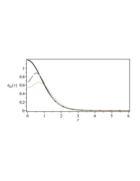
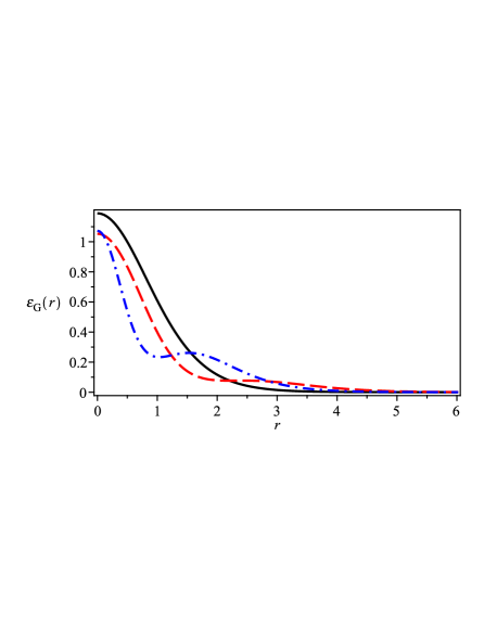
Figure 6: Numerical solutions to the energy distribution $\varepsilon_{G}$ related to the BPS configurations. Conventions as in the Fig. 1. Note how the source field changes the shape of the resulting profiles.

The numerical results for the energy density $\varepsilon_{G}$ are shown in the Fig. 6, from which we see how the source field again controls the shape of the corresponding solutions, which eventually mimic the standard’s shape, see the solution for $r_{0}=2$ (i.e. the dashed red one).

We end this Section by verifying how the dielectric medium changes the way the fields of the model behave near the boundaries. In this sense, we solve the equations (40), (41) and (42) around the boundary values (5), (6) and (17), from which we get that the approximate solutions near the origin read (here, we have chosen $n=N>0$),

$$g(r)\approx g_{N}r^{N}-\frac{eB_{0}}{4}g_{N}r^{N+2}\text{,}$$ (43)

$$a(r)\approx N-\frac{eB_{0}}{2}r^{2}\text{,}$$ (44)

$$A_{0}(r)\approx w_{0}-\frac{\kappa B_{0}}{4}r^{2}\text{,}$$ (45)

where $g_{N}>0$ and $w_{0}$ are integration constants, and $B_{0}$ is the same parameter already defined in the Eq. (36). In the meantime, the asymptotic solutions can be verified to be given by

$$g(r)\approx 1-C_{\infty}\frac{e^{-Mr}}{\sqrt{r}}\text{,}$$ (46)

$$a(r)\approx MC_{\infty}\sqrt{r}e^{-Mr}\text{,}$$ (47)

$$A_{0}(r)\approx\frac{MC_{\infty}}{e}\frac{e^{-Mr}}{\sqrt{r}}\text{,}$$ (48)

which therefore recover the typical behavior (i.e., the exponential decay). In this case, we have identified

$$M=\frac{1}{2}\sqrt{8e^{2}v^{2}+\kappa^{2}}-\frac{|\kappa|}{2}\text{,}$$ (49)

as the mass of the corresponding bosons. The important observation here is that the dielectric medium (38) does not change the manner the fundamental fields approach the boundaries (remember that the medium equals the unity at the boundaries, i.e. $G(r=0)=1$ and $G(r\rightarrow\infty)\rightarrow 1$). In this sense, the basic fields are expected to mimic the behavior of the ones obtained from the self-dual Maxwell-Chern-Simons-Higgs model in the absence of the dielectric medium.

III The Maxwell-Chern-Simons-$CP(2)$ case

We now go further in our investigation by focusing our attention on the first-order vortices with internal structure inherent to an extended Maxwell-Chern-Simons-$CP(2)$ theory. Here, it is important to say that the observations introduced during the construction of the self-dual MCSH theory apply again in order to generate a MCS-$CP(2)$ self-dual scenario neyver , including the one related to the formation of the internal structures.

We then begin by considering the Lagrange density which describes the extended MCS-$CP(2)$ model, i.e.

$$\mathcal{L} = -\frac{G(\chi)}{4}F_{\mu\upsilon}F^{\mu\upsilon}-\frac{\kappa}{4}\epsilon^{\beta\mu\upsilon}A_{\beta}F_{\mu\upsilon}$$ (50)

$$+\overline{\left(P_{ab}D_{\mu}\phi_{b}\right)}\left(P_{ac}D^{\mu}\phi_{c}\right)+\frac{G(\chi)}{2}\partial_{\mu}\Psi\partial^{\mu}\Psi$$

$$+\frac{1}{2}\partial_{\mu}\chi\partial^{\mu}\chi-U\left(\phi_{3},\Psi,\chi\right)\text{,}$$

where the Latin indexes count the components of the $CP(2)$ sector, $\phi_{a}$ represents the $CP(2)$ field which is constrained to satisfy the condition $\phi_{a}\overline{\phi}_{a}=h$ (the constant $h$ represents the norm of the field), $P_{ab}=\delta_{ab}-h^{-1}\phi_{a}\overline{\phi}_{b}$ stands for a projector in the internal space and $D_{\mu}\phi_{a}$ is the covariant derivative of the model, i.e.

$$D_{\mu}\phi_{a}=\partial_{\mu}\phi_{a}-igA_{\mu}Q_{ab}\phi_{b}\text{,}$$ (51)

where $g$ is a coupling constant and $Q_{ab}$ stands for a charge matrix that, for our purpose, we choose as

$$Q_{ab}=\frac{1}{2}\text{diag}\left(1,-1,0\right)\text{.}$$ (52)

The remaining definitions and conventions are the same as in the previous Section.

The potential reads as

$$U\left(\phi_{3},\Psi,\chi\right) = \frac{1}{2G}\left(h^{1/2}g\phi_{3}+\kappa\Psi\right)^{2}$$ (53)

$$+g^{2}\Psi^{2}\overline{\left(P_{ab}Q_{bm}\phi_{m}\right)}P_{ac}Q_{cn}\phi_{n}$$

$$+\frac{1}{2r^{2}}\left(\frac{dW}{d\chi}\right)^{2}\text{,}$$

where the first two terms in the right-hand side (with $G=1$) represent the self-dual potential inherent to the canonical MCS-$CP(2)$ theory neyver . The dependence of the potential on the third component of the $CP(2)$ field presupposes the spontaneous breaking of $SU(3)$-symmetry inherent to the model. On the other hand, the presence of the Chern-Simons term justifies the obtainment of solutions with internal structure carrying on both electric and magnetic fields.

We consider time-independent configurations described by the map

$$A_{i}=-\frac{1}{gr^{2}}\varepsilon_{ij}x_{j}A(r)\text{,}$$ (54)

$$\left(\begin{array}[]{c}\phi_{1}\\ \phi_{2}\\ \phi_{3}\end{array}\right)=h^{\frac{1}{2}}\left(\begin{array}[]{c}e^{im\theta}\sin\alpha\cos\beta\\ e^{-im\theta}\sin\alpha\sin\beta\\ \cos\alpha\end{array}\right)\text{,}$$ (55)

where $\alpha=\alpha(r)$ and $\beta=\beta(r)$ are a priori functions of the radial coordinate $r$ only. Here, the vorticity of the final solutions is determined by the winding number $m=\pm 1,\,\pm 2,\,\pm 3...$, while the above map again leads us to $A_{0}=A_{0}(r)$, $\Psi=\Psi(r)$ and $\chi=\chi(r)$.

It is useful to emphasize that the presence of the source field $\chi$ does not change the equation of motion for $\beta(r)$ which still reads as in the Eq. (17) of the Ref. neyver . Thus, one again gets that the simplest solutions for $\beta(r)$ are

$$\beta_{1}=\frac{\pi}{4}+\frac{n\pi}{2}\text{ \ and \ }\beta_{2}=\frac{n\pi}{2}\text{,}$$ (56)

with $n\in\mathbb{Z}$. In this section, we work with the first choice only, i.e. $\beta(r)=\beta_{1}$.

Furthermore, the other field profiles $\alpha(r)$ and $A(r)$ are supposed to satisfy the same boundary conditions as they do in the absence of the dielectric medium, i.e.

$$\alpha\left(r=0\right)=0\text{ \ and \ }A\left(r=0\right)=0\text{,}$$ (57)

$$\alpha\left(r\rightarrow\infty\right)\rightarrow\frac{\pi}{2}\text{ \ and \ }A\left(r\rightarrow\infty\right)\rightarrow 2m\text{,}$$ (58)

which are known to lead to well-behaved solutions with finite energy.

We proceed with the minimization of the total energy again via the implementation of the BPS algorithm. In order to attain this goal, we first write the expression for the energy density related to the model (50), which reads

$$\varepsilon = \frac{G}{2}B^{2}+\frac{G}{2}\left(\frac{dA_{0}}{dr}\right)^{2}$$ (59)

$$+h\left(\left(\frac{d\alpha}{dr}\right)^{2}+\frac{\left(2m-A\right)^{2}}{4r^{2}}\sin^{2}\alpha\right)$$

$$+\frac{g^{2}h}{4}\left(A_{0}\right)^{2}\sin^{2}\alpha+\frac{G}{2}\left(\frac{d\Psi}{dr}\right)^{2}$$

$$+\frac{1}{2}\left(\frac{d\chi}{dr}\right)^{2}+\frac{1}{2G}\left(hg\cos\alpha+\kappa\Psi\right)^{2}$$

$$+\frac{h}{4}g^{2}\Psi^{2}\sin^{2}\alpha+\frac{1}{2r^{2}}\left(\frac{dW}{d\chi}\right)^{2}\text{,}$$

where we have used the Eq. (53) for the potential $U=U(\phi_{3},\Psi,\chi)$ and the radially symmetric map (54) and (55), with $\beta(r)=\beta_{1}$. In the sequence, after some algebraic work, the above expression can be written in the form

$$\varepsilon = \varepsilon_{BPS}+\frac{1}{2G}\left(\frac{{}}{{}}GB\mp\left(hg\cos\alpha+\kappa\Psi\right)\right)^{2}$$ (60)

$$+h\left[\frac{d\alpha}{dr}\mp\frac{\left(2m-A\right)}{2r}\sin\alpha\right]^{2}+\frac{1}{2}\left(\frac{d\chi}{dr}\mp\frac{1}{r}\frac{dW}{d\chi}\right)^{2}\$$

$$+\frac{1}{2}G\left(\frac{dA_{0}}{dr}\pm\frac{d\Psi}{dr}\right)^{2}+\frac{g^{2}h}{4}\left(A_{0}\pm\Psi\right)^{2}\sin^{2}\alpha\text{,}$$

in which we have again introduced the term $\varepsilon_{BPS}$ which is now given by

$$\varepsilon_{BPS}=\mp\frac{1}{r}\frac{d}{dr}\left[h\left(2m-A\right)\cos\alpha\right]\pm\frac{1}{r}\frac{dW}{dr}\text{,}$$ (61)

whose integration over the plane, using the boundary values (57) and (58), provides the quantity that stands for the BPS energy of the model (50), i.e.

$$E_{BPS}=2\pi\int_{0}^{\infty}r\varepsilon_{BPS}dr=\pm 2\pi\left(2mh+\Delta W\right)\text{,}$$ (62)

where $\Delta W=W\left(r\rightarrow\infty\right)-W(r=0)$, while the upper (lower) sign holds for $m>0$ and $\Delta W>0$ ($m<0$ and $\Delta W<0$).

The construction above reveals that the total energy satisfies

$$\left.\frac{E}{2\pi}=\int_{0}^{\infty}\frac{1}{2G}\left(\frac{{}}{{}}GB\mp\left(hg\cos\alpha+\kappa\Psi\right)\right)^{2}rdr\right.$$

$$\left.+\int_{0}^{\infty}\left[h\left(\frac{d\alpha}{dr}\mp\frac{\left(2m-A\right)}{2r}\sin\alpha\right)^{2}\right.\right.$$

$$\left.\text{ \ \ \ \ \ \ \ \ \ \ \ \ \ \ \ \ \ \ \ \ \ \ \ \ \ \ \ \ \ }\left.+\frac{1}{2}\left(\frac{d\chi}{dr}\mp\frac{1}{r}\frac{dW}{d\chi}\right)^{2}\right]rdr\right.$$

$$\left.+\int_{0}^{\infty}\left[\frac{G}{2}\left(\frac{dA_{0}}{dr}\pm\frac{d\Psi}{dr}\right)^{2}+\frac{g^{2}h}{4}\left(A_{0}\pm\Psi\right)^{2}\sin^{2}\alpha\right]rdr\right.$$

$$\left.+\frac{E_{BPS}}{2\pi}\geq 2h\left|m\right|+\left|\Delta W\right|\right.$$ (63)

and that it is therefore bounded from below. In this sense, the fields which saturate the bound are necessarily the ones which satisfy the following system of equations

$$GB=\pm hg\cos\alpha\pm\kappa\Psi\text{,}$$ (64)

$$\frac{d\alpha}{dr}=\pm\frac{\left(2m-A\right)}{2r}\sin\alpha\text{,}$$ (65)

$$\frac{d\chi}{dr}=\pm\frac{1}{r}\frac{dW}{d\chi}\text{,}$$ (66)

$$\frac{dA_{0}}{dr}=\mp\frac{d\Psi}{dr}\text{ \ and \ }A_{0}=\mp\Psi\text{,}$$ (67)

which provides the first-order equations inherent to the effective theory. In other words, the fields which solve these differential equations originate BPS vortices whose total energy is given by the Eq. (62), i.e. the corresponding Bogomol’nyi bound.

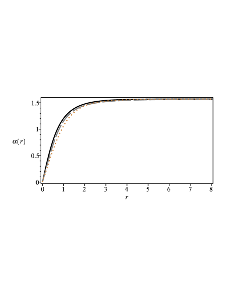
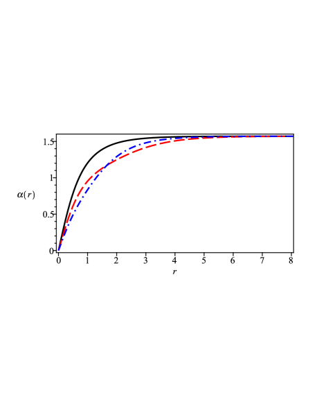
Figure 7: Numerical solutions to the scalar profile function $\alpha(r)$ coming from (73), (74) and (75) (top, long-dashed gray line for $r_{0}=1$ and dotted orange line for $r_{0}=2$) and (86), (87) and (88) (bottom, dash-dotted blue line for $r_{0}=1$ and dashed red line for $r_{0}=2$). In both cases, the equations were solved according the boundary conditions (57), (58) and (17). We have used $h=\kappa=1$, $g=2$ and $m=1$. The solid black line represents the canonical solution (no source field, with $G=1$).

In the same way as in the previous case, the last first-order equation, $\Psi=\mp A_{0}$, solves the penultimate one, $\Psi^{\prime}=\mp A_{0}^{\prime}$, identically. In addition, the electric potential must be again obtained by solving the time-independent Gauss law,

$$\frac{1}{r}\frac{d}{dr}\left(rG\frac{dA_{0}}{dr}\right)+\kappa B=\frac{g^{2}h}{2}A_{0}\sin^{2}\alpha\text{,}$$ (68)

with $A_{0}(r)$ satisfying the same boundary conditions given in the Eq. (17).

Furthermore, it is possible to express the BPS energy density (61) in the same way as in (21), with $\varepsilon_{G}$ representing the contribution which comes from the $CP(2)$ soliton with internal structure, i.e.

$$\varepsilon_{G} = G\left[B^{2}+\left(\frac{dA_{0}}{dr}\right)^{2}\right]$$ (69)

$$\text{ \ \ \ \ }+\frac{h}{2}\left[g^{2}\left(A_{0}\right)^{2}+\frac{(2m-A)^{2}}{r^{2}}\right]\sin^{2}\alpha\text{,}$$

and $\varepsilon_{\chi}$ standing for the energy density of the source field $\chi$ given again by the Eq. (23).

III.1 Some MCS-$CP(2)$ scenarios with internal structure

We proceed in the same way as in the Sec. II in order to introduce some first-order scenarios. In this sense, for comparison purposes, we choose the superpotential $W(\chi)$ again as it appears in the Eq. (18) of the previous Sec. II.1, i.e.

$$W(\chi)=\chi-\frac{1}{3}\chi^{3}\text{,}$$ (70)

which, in view of the Eq. (66), provides the solution for the source field as given in the Eq. (20), i.e.

$$\chi(r)=\pm\frac{r^{2}-r_{0}^{2}}{r^{2}+r_{0}^{2}}\text{.}$$ (71)

III.1.1 The first case

Now, we specify the dielectric function $G(\chi)$. Here, in order to to compare the corresponding effects with the ones observed previously in the MCSH case, we choose this function as in the Eq. (24) or, alternatively, as in the Eq. (25),

$$G(\chi)=\frac{1}{1-\chi^{2}}=\frac{\left(r^{2}+r_{0}^{2}\right)^{2}}{4r^{2}r_{0}^{2}}\text{,}$$ (72)

whose peculiarities were already discussed in the previous Section II.1.1.

In view of (72), the first-order equations (64) and (65) reduce to

$$\frac{1}{r}\frac{dA}{dr}=\frac{4r^{2}r_{0}^{2}}{\left(r^{2}+r_{0}^{2}\right)^{2}}\left(\pm hg^{2}\cos\alpha-g\kappa A_{0}\right)\text{,}$$ (73)

$$\frac{d\alpha}{dr}=\pm\frac{\left(2m-A\right)}{2r}\sin\alpha\text{,}$$ (74)

while the Gauss law assumes the form

$$\frac{1}{4r_{0}^{2}r}\frac{d}{dr}\left[\frac{\left(r^{2}+r_{0}^{2}\right)^{2}}{r}\frac{dA_{0}}{dr}\right]+\kappa B=\frac{g^{2}h}{2}A_{0}\sin^{2}\alpha\text{,}$$ (75)

where $B$ represents the magnetic field given by

$$B(r)=\frac{1}{gr}\frac{dA}{dr}\text{.}$$ (76)

We perform the numerical analysis again by using a finite-difference scheme and according the conditions (57), (58) and (17). Here, we choose $h=\kappa=1$, $g=2$, and $m=1$ (upper signs in the first-order expressions). We then solve the BPS equations (73), (74) and (75) for $r_{0}=1$ (long-dashed gray line) and $r_{0}=2$ (dotted orange line), from which we depict the numerical profile for the fields $\alpha(r)$ and $A(r)$, the electric potential $A_{0}(r)$, the magnetic $B(r)$ and electric $E(r)$ fields, and the energy distribution $\varepsilon_{G}$, see the figures 7-12 (the solid black line stands for the solution with no source field, i.e. $G=1$).

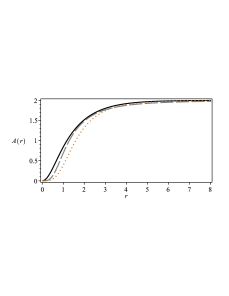
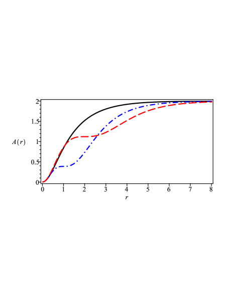
Figure 8: Numerical solutions to the gauge profile function $A(r)$. Conventions as in the Fig. 7. The solutions for the 1st. case mimic the usual ones around $r=r_{0}$, while the profiles for the 2nd. case present a plateau at the same point.

In this sense, the field profiles $\alpha(r)$ and $A(r)$ are shown in the figures 7 and 8, respectively. In view of them, it’s possible to note that the presence of the source field causes slight variations on the respective core-size. Also here, the profiles converge to the boundary values (57) and (58) despite the presence of the dielectric medium itself.

The Figure 9 shows the solutions for the electric potential $A_{0}(r)$, from which one notes that the behavior of $A_{0}(r=0)=w_{0}$ as a function of $r_{0}$ is the very similar to the one which we have already encountered in the previous MCSH case (see the Fig. 3), i.e. as $r_{0}$ increases, $w_{0}$ decreases.

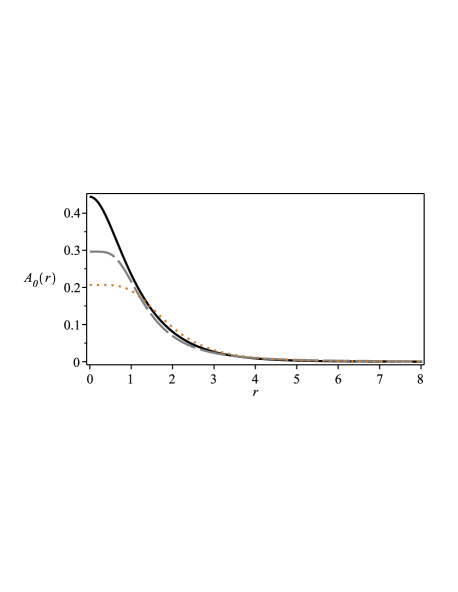
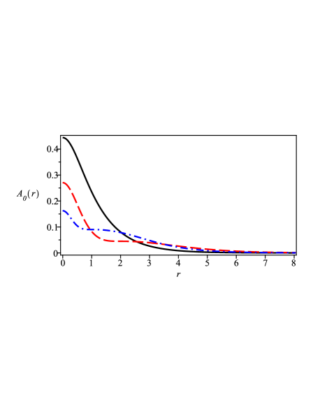
Figure 9: Numerical solutions to the electric potential $A_{0}(r)$. Conventions as in the 7. The solutions for the 1st. case mimic the standard behavior around $r=r_{0}$. The results for the 2nd. case also have a plateau at the same point.

The solutions for the magnetic and electric fields can be seen in figures 10 and 11, respectively. We see that the dielectric medium causes the very same effect already observed in the MCSH case, i.e. the magnetic and electric fields vanish at the boundaries to ensure that the energy of the resulting BPS vortices converges to the bound given by the Eq. (62).

The Figure 12 presents the solutions for the energy density $\varepsilon_{G}$ of the first-order vortices, via which one gets that again the presence of the source field changes the shape of the resulting profiles. Moreover, as it happens for the electric potential, as the values of $r_{0}$ increase, the values of $\varepsilon_{G}(r=0)$ decrease.

We finalize the study of this case by solving the first-order system (73), (74) and (75) near to the boundary conditions (57), (58) and (17). So, around the boundary $r=0$, we solve for $m=1$ (the case analyzed numerically), which provides the following behavior for the field profiles:

$$\alpha(r)\approx\alpha_{1}r-\frac{\left(\alpha_{1}\right)^{3}}{12}r^{3}\text{,}$$ (77)

$$A(r)\approx\frac{g\tilde{B}_{0}}{r_{0}^{2}}r^{4}-\left(\frac{gA_{1}}{3r_{0}^{2}}+\frac{4g\tilde{B}_{0}}{3r_{0}^{4}}\right)r^{6}\text{,}$$ (78)

$$A_{0}(r)\approx w_{0}+w_{2}r^{2}\text{,}$$ (79)

where $\alpha_{1}$ and $w_{2}$ stand for positive integration constants, with $A_{1}=2w_{2}\kappa+gh\left(\alpha_{1}\right)^{2}$ and

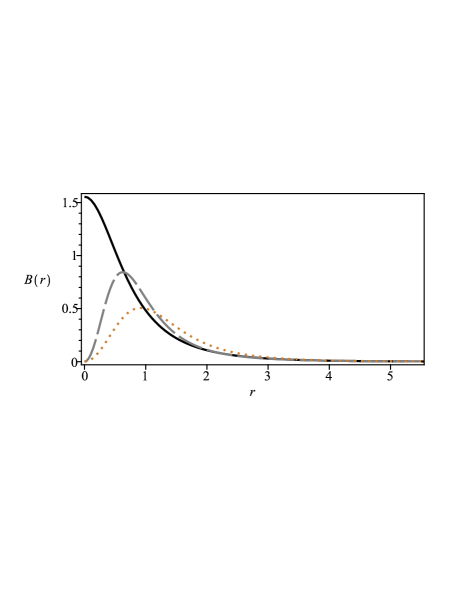
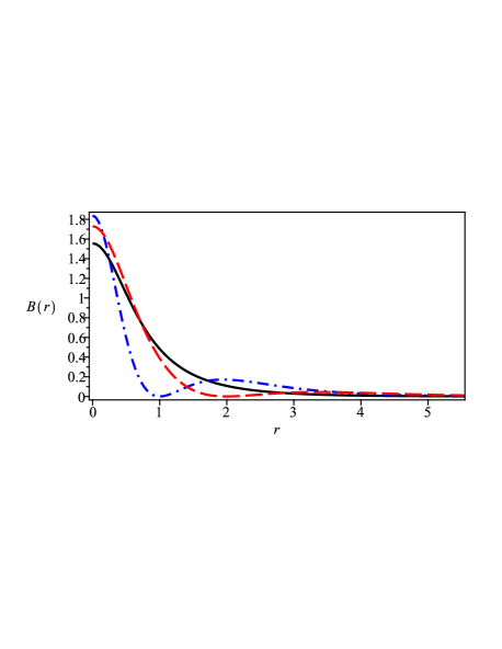
Figure 10: Numerical solutions to the magnetic field $B(r)$. Conventions as in the 7. The solutions for the 2nd. case vanish at $r=r_{0}$ in order to avoid the first term in the right-hand side of the Eq. (59) to be singular.

$$\tilde{B}_{0}=hg-w_{0}\kappa\text{,}$$ (80)

which stands for the value of the magnetic field at $r=0$ for the MCS-$CP(2)$ model in the absence of the dielectric medium. On the other hand, in the limit $r\rightarrow\infty$, we obtain

$$\alpha(r)\approx\frac{\pi}{2}-C_{\infty}r^{-\Lambda}\text{,}$$ (81)

$$A(r)\approx 2m-2\Lambda C_{\infty}r^{-\Lambda}\text{,}$$ (82)

$$A_{0}(r)\approx-\frac{\Lambda C_{\infty}}{g\kappa\left(r_{0}\right)^{2}}r^{-\Lambda}\text{,}$$ (83)

which hold for an arbitrary $m>0$ ($C_{\infty}$ is a positive integration constant). Here, we have defined

$$\Lambda=1+\sqrt{1+2h\left(gr_{0}\right)^{2}}$$ (84)

as the parameter which controls the way the basic fields approach the boundary $r\rightarrow\infty$. It is interesting to note that the source field gives rise to the very same asymptotic behavior also found in the previous MCSH case, including the dependence of the parameter $\Lambda$ on the values of $r_{0}$, see the Eq. (37).

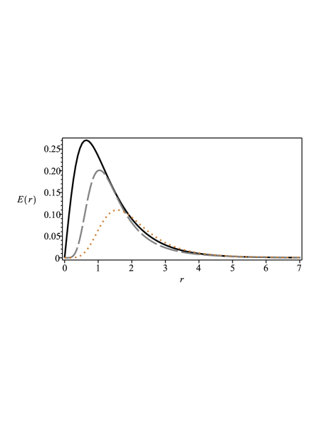
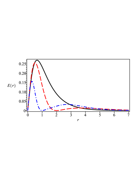
Figure 11: Numerical solutions to the electric field $E(r)$. Conventions as in the 7. The solutions for the 2nd. case vanish at $r=r_{0}$ in order to avoid the second term in the right-hand side of the Eq. (59) to be singular.

III.1.2 The second case

We finally study the effects induced on the MCS-$CP(2)$ solitons by the second choice for $G(\chi)$ introduced in the Eq. (38) and explicitly given in terms of $r$ by the Eq. (39), i.e.

$$G(\chi)=\frac{1}{\chi^{2}}=\frac{\left(r^{2}+r_{0}^{2}\right)^{2}}{\left(r^{2}-r_{0}^{2}\right)^{2}}\text{.}$$ (85)

As already commented in the context of the MCSH case, its influence at the boundaries disappears, from which the behavior of the corresponding solitons is expected to mimic the one which emerges in the absence of the dielectric medium. Furthermore, the electric and magnetic fields vanish at $r=r_{0}$, then the first two terms in the right-hand side of the Eq. (59) are expected to be nonsingular.

In this case, the first-order equations (64) and (65) are written, respectively, as

$$\frac{1}{r}\frac{dA}{dr}=\frac{\left(r^{2}-r_{0}^{2}\right)^{2}}{\left(r^{2}+r_{0}^{2}\right)^{2}}\left(\pm hg^{2}\cos\alpha-g\kappa A_{0}\right)\text{,}$$ (86)

$$\frac{d\alpha}{dr}=\pm\frac{\left(2m-A\right)}{2r}\sin\alpha\text{,}$$ (87)

while the Gauss law reads

$$\frac{1}{r}\frac{d}{dr}\left[\frac{\left(r^{2}+r_{0}^{2}\right)^{2}r}{\left(r^{2}-r_{0}^{2}\right)^{2}}\frac{dA_{0}}{dr}\right]+\kappa B=\frac{g^{2}h}{2}A_{0}\sin^{2}\alpha\text{,}$$ (88)

where the magnetic field $B$ is again given by the Eq. (76).

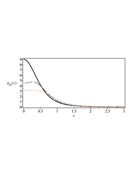
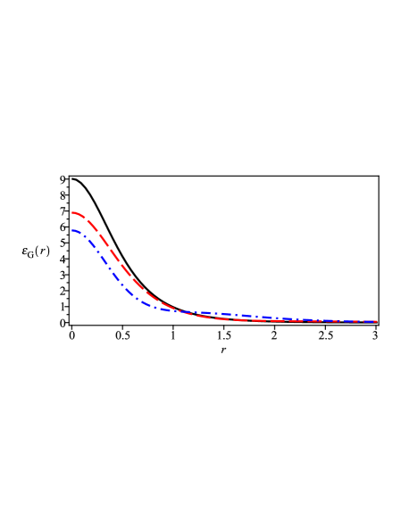
Figure 12: Numerical solutions to the energy distribution $\varepsilon_{G}$ related to the BPS configurations. Conventions as in the Fig. 7. The source field eventually changes the shape of the resulting profiles.

With the aim to compare the new results with the ones achieved previously, we again set $h=\kappa=1$, $g=2$ and $m=1$, from which we solve the differential equations (86), (87) and (88) for $r_{0}=1$ (dash-dotted blue line) and $r_{0}=2$ (dashed red line) according the conditions (57), (58) and (17). We plot the resulting profiles in the corresponding figures 7-12.

The resulting profiles for $\alpha(r)$, $A(r)$ and $A_{0}(r)$ appear in the figures 7, 8, and 9, respectively, via which we see that again both the gauge profile function and the electric potential present the formation of a plateau in the neighborhood of $r=r_{0}$. As the reader can expect based on our previous discussions, these structures force both the magnetic and electric field to vanish at this particular point (see the figures 10 and 11, respectively), a similar effect to the one observed previously in the MCSH case. Thus, they guarantee that the energy of the first-order configurations converges to the value given by the Eq. (62).

The Figure 12 brings the profiles which we have found for the energy density $\varepsilon_{G}$, from which we see that even in the presence of the source field the new solutions mimic the same general shape presented by the canonical configurations.

We end this study by investigating the behavior of the solutions near the boundaries. In this sense, by solving the equations (86), (87) and (88) around to the origin, we obtain that the fields behave as

$$\alpha(r)\approx\alpha_{1}r-\left[\frac{\left(\alpha_{1}\right)^{3}}{12}+\frac{g\tilde{B}_{0}}{8}\alpha_{1}\right]r^{3}\text{,}$$ (89)

$$A(r)\approx\frac{g\tilde{B}_{0}}{2}r^{2}-\tilde{A}_{1}r^{4}\text{,}$$ (90)

$$A_{0}(r)\approx w_{0}-\frac{\kappa\tilde{B}_{0}}{4}r^{2}\text{,}$$ (91)

with the expressions above holding for $m=1$, the winding number analyzed in this work. The quantity $\tilde{B}_{0}$ was already defined in the Eq. (80). Here, we have also introduced the parameter $\tilde{A}_{1}$ defined by

$$\tilde{A}_{1}=\frac{g^{2}h}{8}(\alpha_{1})^{2}-\frac{g\tilde{B}_{0}}{16}\left(\kappa^{2}-\frac{16}{r_{0}^{2}}\right)\text{.}$$ (92)

The approximate solutions for $r\rightarrow\infty$ read as

$$\alpha(r)\approx\frac{\pi}{2}-C_{\infty}\frac{e^{-Mr}}{\sqrt{r}}\text{,}$$ (93)

$$A(r)\approx 2m-2MC_{\infty}\sqrt{r}\,e^{-Mr}\text{,}$$ (94)

$$A_{0}(r)\approx\frac{2MC_{\infty}}{g}\frac{e^{-Mr}}{\sqrt{r}}\text{,}$$ (95)

which are valid for $m>0$. In this case, we have defined

$$M=\frac{1}{2}\sqrt{2hg^{2}+\kappa^{2}}-\frac{\left|\kappa\right|}{2}\text{,}$$ (96)

which stands for the mass of the corresponding bosons. In view of these asymptotic solutions, we conclude that, as in the previous MCSH scenario, the presence of the dielectric medium does not change the way the basic fields approach their boundary values, at least at relevant orders of $r$.

IV Summary and perspectives

We have investigated the formation of BPS vortices with internal structures in both the Maxwell-Chern-Simons-Higgs and the Maxwell-Chern-Simons-$CP(2)$ scenarios. The internal structures are generated through the introduction of a dielectric medium which is driven by an extra real scalar field (named the source field) which extends both the original models. We have then focused our attention on time-independent radially symmetric configurations with a self-dual structure. In order to attain such a goal, we have proceeded with the implementation of the Bogomolnyi-Prasad-Sommerfield algorithm which has allowed us to obtain the Bogomol’nyi bound and the self-dual BPS equations for both the models analyzed in this manuscript.

In the sequence, we have observed that the self-dual equation for the source field depends only on the particular choice for the superpotential $W(\chi)$ and that therefore this equation decouples from the others BPS equations of the model. For a specific superpotential, the self-dual solution for $\chi(r)$ allows us to define a dielectric function $G(\chi)$ which becomes responsible for the generation of the internal structures inherent to the new first-order vortices. We have splitted our investigation into two different branches based on the functional forms which we have chosen for the dielectric function $G(\chi)$ which appears in the Lagrange densities of the models.

We have finally solved the remaining BPS equations together with the Gauss law by means of a finite-difference scheme according to the canonical boundary conditions. The numerical results have verified that the presence of the dielectric medium induces similar effects in both scenarios.

In view of the numerical analysis, we have observed that the dielectric causes different effects on the corresponding vortex profiles in comparison to the ones obtained in the absence of if. This way, the first choice $G(\chi)=(1-\chi^{2})^{-1}$ changes the way the magnetic and electric fields behave near the boundaries. On the other hand, the second choice $G(\chi)=\chi^{-2}$ affects the manner the fields behave along the radial coordinate, except near the boundary values. In particular, the second choice for the dielectric function leads to magnetic and electric fields which vanish at $r=r_{0}$. This particular behavior ensures that the energy of the self-dual BPS vortices converge to the finite Bogomol’nyi bound.

An interesting perspective is the application of the present idea to the Maxwell-Skyrme system, or the study of the MCS-$CP(2)$ vortices with an unusual shape caused by the inclusion of a magnetic impurity, see the references 15 and 19 , for instance. These issues are currently under investigation and the results we will be reported in a future contribution.

- (1) N. Manton and P. Sutcliffe, Topological Solitons (Cambridge University Press, Cambridge, England, 2004).
- (2) E. Bogomol’nyi, Sov. J. Nucl. Phys. 24, 449 (1976). M. Prasad and C. Sommerfield, Phys. Rev. Lett. 35, 760 (1975).
- (3) H. J. de Vega and F. A. Schaposnik, Phys. Rev. D 14, 1100 (1976).
- (4) A. N. Atmaja and H. S. Ramadhan, Phys. Rev. D 90, 105009 (2014). A. N. Atmaja, H. S. Ramadhan and E. da Hora, J. High Energy Phys. 1602, 117 (2016).
- (5) H. B. Nielsen and P. Olesen, Nucl. Phys. B 61, 45 (1973).
- (6) R. Jackiw and E. J. Weinberg, Phys. Rev. Lett. 64, 2234 (1990). R. Jackiw, K. Lee and E. J. Weinberg, Phys. Rev. D 42, 3488 (1990).
- (7) C. Lee, K. Lee and H. Min, Phys. Lett. B 252, 79 (1990).
- (8) A. Yu. Loginov, Phys. Rev. D 93, 065009 (2016).
- (9) R. Casana, M. L. Dias and E. da Hora, Phys. Lett. B 768, 254 (2017).
- (10) V. Almeida, R. Casana and E. da Hora, Phys. Rev. D 97, 016013 (2018). R. Casana, M. L. Dias and E. da Hora, Phys. Rev. D 98, 056011 (2018).
- (11) R. Casana, N. H. Gonzalez-Gutierrez and E. da Hora, Europhys. Lett. 127, 61001 (2019).
- (12) E. Witten, Nucl. Phys. B 249, 557 (1985). M. Shifman, Phys. Rev. D 87, 025025 (2013). A. Peterson, M. Shifman and G. Tallarita, Annals Phys. 353, 48 (2014); Annals Phys. 363, 515 (2015).
- (13) D. Bazeia, M. A. Marques and R. Menezes, Phys. Lett. B 780, 485 (2018).
- (14) R. A. Shelby, Science 292, 77 (2001). S. A. Ramakrishna, Rep. Prog. Phys. 68, 449 (2005). C. Caloz, Metamater. Today 12, 12 (2009).
- (15) J. Andrade, R. Casana, E. da Hora and C. dos Santos, Phys. Rev. D 99, 056014 (2019).
- (16) D. Bazeia, M. M. Doria and E. I. B. Rodrigues, Phys. Lett. A 380, 1947 (2016). D. Bazeia, J. G. G. S. Ramos and E. I. B. Rodrigues, J. Magnetism Magnetic Materials 423, 411 (2017).
- (17) D. Bazeia and A. Mohammadi, Phys. Lett. B 779, 420 (2018).
- (18) D. Tong and K. Wong, J. High Energy Phys. 1401, 090 (2014).
- (19) A. Cockburn, S. Krusch and A. A. Muhamed, J. Math. Phys. 58, 063509 (2017). J. Ashcroft and S. Krusch, Phys. Rev. D 101, 025004 (2020).