TRICE: A Channel Estimation Framework for RIS-Aided Millimeter-Wave MIMO Systems

Abstract

We consider the channel estimation problem in point-to-point reconfigurable intelligent surface (RIS)-aided millimeter-wave (mmWave) MIMO systems. By exploiting the low-rank nature of mmWave channels in the angular domains, we propose a non-iterative Two-stage RIS-aided Channel Estimation (TRICE) framework, where every stage is formulated as a multidimensional direction-of-arrival (DOA) estimation problem. As a result, our TRICE framework is very general in the sense that any efficient multidimensional DOA estimation solution can be readily used in every stage to estimate the associated channel parameters. Numerical results show that the TRICE framework has a lower training overhead and a lower computational complexity, as compared to benchmark solutions.

I Introduction

Reconfigurable intelligent surfaces (RISs) have been proposed recently as a cost-effective technology for reconfiguring the wireless propagation channel between transceivers [1, 2, 3, 4, 5, 6, 7]. In RIS-aided systems, an accurate channel state information (CSI) is required at transceivers to enable efficient signal processing techniques, e.g., beamforming and resource allocation. However, the acquisition of CSI in such systems faces several challenges. For instance, assuming a passive RIS implementation, to reduce the RIS cost and complexity, the propagation channel can only be sensed and estimated at the receiver. Furthermore, the large number of channel coefficients to be estimated limits the feasibility of CSI acquisition within a practical coherence time, since an RIS is expected to have a massive number of passive reflecting elements. Recently, channel estimation methods for RIS-aided systems have been proposed, e.g., using least-squares (LS) based methods as in [8, 9, 10, 11], or minimum mean squared error based methods as in [12]. However, these works require the number of training subframes to be, at least, equal to the number of RISs reflecting elements, which is a limiting factor in practice.

In millimeter-wave (mmWave) communications [13, 14, 15, 16, 17, 18], it was observed that the MIMO propagation channel has a low-rank structure, due to the small number of scatterers. Such a low-rank structure can be exploited to reduce the channel training overhead and complexity, as it has been shown in [19, 20, 21, 22, 23, 24]. In these works, every channel matrix is modeled as a summation of $L$ paths, where $L$ is much smaller than the number of transmit and receiver antennas, and every path is completely characterized by a direction-of-departure (DOD), a direction-of-arrival (DOA), and a complex path gain. Therefore, the channel estimation is formulated as a sparse recovery problem, for which compressed sensing (CS) techniques [25] can be used to efficiently recover the channel parameters using a small training overhead. In [19], the above problem is facilitated by assuming that the RIS has a few active elements, which, however, increases the deployment cost and the energy consumption of RIS-aided systems. In [20], the authors assumed that the base station (BS)-to-RIS channel is perfectly known, while in [21], the cascade channel matrix is assumed to have a single path, i.e., $L=1$. Differently, the authors in [24] proposed a general sparse recovery formulation for $L\geq 1$ scenarios. In most of these works, however, the channel parameters are assumed to fall perfectly on a grid, which may never be true in practice. Therefore, there exists a trade-off between the estimation accuracy and the complexity, where both increase as a function of the grid resolution. Due to the multidimensionality of the cascaded channel, a 4D sensing matrix is required by the method proposed in [24], which makes it computationally prohibitive even with low grid resolutions.

In this paper, we consider the channel estimation problem in a single-user RIS-aided mmWave MIMO communication system, similarly to [24], where the RIS has passive reflecting elements and the direct link between the BS and the mobile station (MS) is assumed to be blocked or pre-estimated by turning the RIS elements off, as in [8]. Using a structured channel training procedure, we propose a Two-Stage RIS-aided Channel Estimation (TRICE) framework for single-user mmWave MIMO communication systems. In the first stage, the DODs of the BS-to-RIS channel and the DOAs of the RIS-to-MS channel are first estimated. In the second stage, by using the estimated channel parameters in the first stage, the effective azimuth and elevation angles of the cascaded BS-to-RIS-to-MS channel at the RIS are estimated, one-by-one, including the effective complex path gains. In both stages, we show that the parameter estimation can be carried out via a multidimensional DOA estimation scheme, for which several solutions exist as in [26, 27, 28, 29, 30, 31], among many others. Detailed simulation results are provided, showing that the proposed TRICE framework has a lower training overhead and a lower computational complexity, as compared to benchmark methods.

II System and Channel Models

In this paper, we consider a single-user mmWave MIMO communication system as depicted in Fig. 1, where a BS equipped with $M_{\text{T}}$ antennas and $N_{\text{T}}\leq M_{\text{T}}$ RF chains is communicating with a MS that has $M_{\text{R}}$ antennas and $N_{\text{R}}\leq M_{\text{R}}$ RF chains. We assume that the direct link between the BS and the MS is unavailable (e.g., due to blockage) and the indirect link is aided by an RIS composed by $M_{\text{S}}$ phase shifters, which are arranged uniformly on a rectangular surface with $M^{\text{v}}_{\text{S}}$ vertical and $M^{\text{h}}_{\text{S}}$ horizontal elements such that $M_{\text{S}}=M^{\text{v}}_{\text{S}}\cdot M^{\text{h}}_{\text{S}}$.

We assume that the BS and the MS employ uniform linear arrays (ULAs). Let $\bm{H}_{\text{T}}\in\mathbb{C}^{M_{\text{S}}\times M_{\text{T}}}$ ($\bm{H}_{\text{R}}\in\mathbb{C}^{M_{\text{R}}\times M_{\text{S}}}$) denotes the mmWave MIMO channel between the BS (RIS) and the RIS (MS). Similarly to [24], $\bm{H}_{\text{T}}$ and $\bm{H}_{\text{R}}$ are modeled according to the classical Saleh-Valenzuela model [32] as

$$\bm{H}_{\text{T}} =\sum_{\ell=1}^{L_{\text{T}}}\alpha_{\text{T},\ell}\bm{v}_{{\text{2D}}}(\mu^{\text{v}}_{\text{T},\ell},\mu^{\text{h}}_{\text{T},\ell})\bm{v}_{{\text{1D}}}(\psi_{\text{T},\ell})^{T}=\bm{B}_{\text{T}}\bm{G}_{\text{T}}\bm{A}^{T}_{\text{T}}$$ (1)

$$\bm{H}_{\text{R}} =\sum_{\ell=1}^{L_{\text{R}}}\alpha_{\text{R},\ell}\bm{v}_{{\text{1D}}}(\psi_{\text{R},\ell})\bm{v}_{{\text{2D}}}(\mu^{\text{v}}_{\text{R},\ell},\mu^{\text{h}}_{\text{R},\ell})^{T}=\bm{A}_{\text{R}}\bm{G}_{\text{R}}\bm{B}^{T}_{\text{R}},$$

where $\alpha_{\text{T},\ell}$ and $\alpha_{\text{R},\ell}$ are the complex path gains, $\psi_{\text{T},\ell}$ ($\psi_{\text{R},\ell}$) is the $\ell$th path DOD (DOA) spatial frequency at the BS (MS), while $\mu^{\text{h}}_{\text{T},\ell}$ and $\mu^{\text{v}}_{\text{T},\ell}$ ($\mu^{\text{h}}_{\text{R},\ell}$ and $\mu^{\text{v}}_{\text{R},\ell}$) are the $\ell$th path azimuth and elevation DOAs (DODs) spatial frequencies at the RIS. Moreover, $\bm{v}_{{\text{2D}}}(\mu^{\text{v}}_{\text{X},\ell},\mu^{\text{h}}_{\text{X},\ell})=\bm{v}_{{\text{1D}}}(\mu^{\text{v}}_{\text{X},\ell})\diamond\bm{v}_{{\text{1D}}}(\mu^{\text{h}}_{\text{X},\ell})\in\mathbb{C}^{M_{\text{S}}}$ and $\bm{v}_{{\text{1D}}}(\psi_{\text{X},\ell})\in\mathbb{C}^{M_{\text{X}}}$ are the functions representing the 2D and the 1D array steering vectors, respectively, where $\text{X}\in\{\text{T},\text{R}\}$. For a given spatial frequency $\nu$, the steering vector $\bm{v}_{{\text{1D}}}(\nu)$ is given as $\bm{v}_{{\text{1D}}}(\nu)=[1,e^{j\nu},\dots,e^{j(M-1)\nu}]^{T}\in\mathbb{C}^{M}.$ In (1), $\bm{H}_{\text{T}}$ and $\bm{H}_{\text{R}}$ are written in a compact form by letting $\bm{A}_{\text{X}}=[\bm{v}_{{\text{1D}}}({\psi}_{\text{X},1}),\dots,\bm{v}_{{\text{1D}}}({\psi}_{\text{X},L_{\text{X}}})]\in\mathbb{C}^{M_{\text{X}}\times L_{\text{X}}}$, $\bm{B}_{\text{X}}=\bm{B}^{\text{v}}_{\text{X}}\diamond\bm{B}^{\text{h}}_{\text{X}}\in\mathbb{C}^{M_{\text{S}}\times L_{\text{X}}}$, $\bm{B}^{\text{y}}_{\text{X}}=[\bm{v}_{{\text{1D}}}({\mu}^{\text{y}}_{\text{X},1}),\dots,\bm{v}_{{\text{1D}}}({\mu}^{\text{y}}_{\text{X},L_{\text{X}}})]\in\mathbb{C}^{M^{\text{y}}_{\text{S}}\times L_{\text{X}}}$, and $\bm{G}_{\text{X}}=\text{diag}\{{\alpha}_{\text{X},1},\dots,{\alpha}_{\text{X},L_{\text{X}}}\}$, where $\text{y}\in\{\text{v},\text{h}\}$.

We assume a block-fading channel, where $\bm{H}_{\text{T}}$ and $\bm{H}_{\text{R}}$ remain constant during each block and change from block to block. To estimate $\bm{H}_{\text{T}}$ and $\bm{H}_{\text{R}}$, we conduct a channel training procedure at the beginning of each block, which comprises $K$ frames divided into $K_{\text{T}}\cdot K_{\text{S}}$ subframes, i.e., $K=K_{\text{S}}\cdot K_{\text{T}}$. At the BS, we assume that a single RF chain is used during the channel training procedure, to reduce the energy consumption, which implies that a single training vector is transmitted in every subframe. Let $\widetilde{\bm{F}}=[\widetilde{\bm{f}}_{1},\dots,\widetilde{\bm{f}}_{K_{T}}]\in\mathbb{C}^{M_{\text{T}}\times K_{\text{T}}}$ be the matrix holding the $K_{\text{T}}$ analog training vectors of the BS, with $\big{|}[\widetilde{\bm{f}}_{t}]_{[i]}\big{|}=\frac{1}{\sqrt{M_{\text{T}}}},\forall t,i$, and $\widetilde{\bm{F}}^{H}\widetilde{\bm{F}}=\bm{I}_{K_{\text{T}}}$. Moreover, let $\bm{Q}=[\bm{q}_{1},\dots,\bm{q}_{K_{\text{S}}}]\in\mathbb{C}^{M_{\text{S}}\times K_{\text{S}}}$ be the matrix holding the $K_{\text{S}}$ phase shift vectors of the RIS, with $\big{|}[{\bm{q}}_{s}]_{[j]}\big{|}=\frac{1}{\sqrt{M_{\text{S}}}},\forall s,j$. We propose to design $\bm{Q}$ to have a Kronecker structure as

$$\bm{Q}=\bm{Q}_{\text{v}}\otimes\bm{Q}_{\text{h}}\in\mathbb{C}^{M_{\text{S}}\times K_{\text{S}}},$$ (2)

where $\bm{Q}_{\text{v}}\in\mathbb{C}^{M^{\text{v}}_{\text{S}}\times K^{\text{v}}_{\text{S}}}$, $\bm{Q}_{\text{h}}\in\mathbb{C}^{M^{\text{h}}_{\text{S}}\times K^{\text{h}}_{\text{S}}}$, and $K_{\text{S}}=K^{\text{v}}_{\text{S}}\cdot K^{\text{h}}_{\text{S}}$. Such a design structure will be exploited in Section III to obtain a low-complexity channel estimation method.

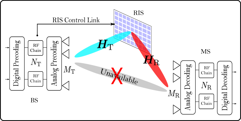
Figure 1: An RIS-aided mmWave MIMO communication system.

The received signal at the MS at the $(s,t)$th subframe, $s\in\{1,\dots,K_{\text{S}}\}$, $t\in\{1,\dots,K_{\text{T}}\}$, is given as

$$\bm{y}_{s,t} =\bm{W}^{T}\bm{H}_{\text{R}}\text{diag}\{\bm{q}_{s}\}\bm{H}_{\text{T}}\widetilde{\bm{f}}_{t}p_{t}+\bm{z}_{s,t}\in\mathbb{C}^{N_{\text{R}}},$$ (3)

where $\bm{W}\in\mathbb{C}^{M_{\text{R}}\times N_{\text{R}}}$ is the decoding matrix, $p_{t}\in\mathbb{C}$ is the unit-power pilot signal, and $\bm{z}_{s,t}\in\mathbb{C}^{N_{\text{R}}}$ is the additive white Gaussian noise vector having zero-mean circularly symmetric complex-valued entries with variance $\sigma^{2}$. Let $\bm{F}=[\widetilde{\bm{f}}_{1}{p}_{1},\dots,\widetilde{\bm{f}}_{K_{T}}{p}_{K_{\text{T}}}]$. Then, by stacking $\bm{y}_{s,t},\forall t$, on top of each other as $\bm{y}_{s}=[\bm{y}^{T}_{s,1},\dots,\bm{y}^{T}_{s,K_{\text{T}}}]^{T}$, we have

$$\bm{y}_{s}=(\bm{F}^{T}\bm{H}^{T}_{\text{T}}\diamond\bm{W}^{T}\bm{H}_{\text{R}})\bm{q}_{s}+\bm{z}_{s}\in\mathbb{C}^{N_{\text{R}}K_{\text{T}}},$$ (4)

where $\bm{z}_{s}=[\bm{z}^{T}_{s,1},\dots,\bm{z}^{T}_{s,K_{\text{T}}}]^{T}$. Let $\bm{H}=(\bm{H}^{T}_{\text{T}}\diamond\bm{H}_{\text{R}})\in\mathbb{C}^{M_{\text{R}}M_{\text{T}}\times M_{\text{S}}}$ and $\bm{Z}=[\bm{z}_{1},\dots,\bm{z}_{K_{\text{S}}}]$. Then, by stacking $\bm{y}_{s},\forall s$, as $\bm{Y}=[\bm{y}_{1},\dots,\bm{y}_{K_{\text{S}}}]$ and applying Property 2, we have

$$\bm{Y}=(\bm{F}^{T}\otimes\bm{W}^{T})\bm{H}\bm{Q}+\bm{Z}\in\mathbb{C}^{N_{\text{R}}K_{\text{T}}\times K_{\text{S}}}.$$ (5)

Our main goal is to estimate $\bm{H}$ from (5). One direct solution is to use the LS-based method. By applying Property 1, the vectorized form of (5) can be written as $\bm{y}=\bm{\Upsilon}\bm{h}+\bm{z}$, where $\bm{\Upsilon}=(\bm{Q}^{T}\otimes\bm{F}^{T}\otimes\bm{W}^{T})\in\mathbb{C}^{N_{\text{R}}K_{\text{T}}K_{\text{S}}\times M_{\text{R}}M_{\text{T}}M_{\text{S}}}$, $\bm{h}=\text{vec}\{\bm{H}\}$, and $\bm{z}=\text{vec}\{\bm{Z}\}$. Therefore, an estimate to the channel vector $\bm{h}$ can be obtained as $\widehat{\bm{h}}_{\text{LS}}=\bm{\Upsilon}^{+}\bm{y}$, which requires $K=K_{\text{T}}K_{\text{S}}\geq\frac{M_{\text{R}}M_{\text{T}}M_{\text{S}}}{N_{\text{R}}}$ to have an accurate channel estimate. Such an approach, however, becomes impractical in a massive MIMO setup, since it requires a large number of training subframes $K$ and a long channel coherence time.

III Proposed TRICE Framework

From (1), the cascaded channel matrix $\bm{H}$ can be written as

$$\bm{H} =(\bm{A}_{\text{T}}\bm{G}_{\text{T}}\bm{B}^{T}_{\text{T}}\diamond\bm{A}_{\text{R}}\bm{G}_{\text{R}}\bm{B}^{T}_{\text{R}})\stackrel{{\scriptstyle\mathclap{\mbox{\tiny(a)}}}}{{=}}(\bm{A}_{\text{T}}\otimes\bm{A}_{\text{R}})\bm{G}\bm{B},$$ (6)

where $\bm{G}=(\bm{G}_{\text{T}}\otimes\bm{G}_{\text{R}})\in\mathbb{C}^{L\times L}$, $\bm{B}=(\bm{B}^{T}_{\text{T}}\diamond\bm{B}^{T}_{\text{R}})\in\mathbb{C}^{L\times M_{\text{S}}}$, $L=L_{\text{R}}{L}_{\text{T}}$, and $\stackrel{{\scriptstyle\mathclap{\mbox{\tiny(a)}}}}{{=}}$ is obtained from Property 2. Using (6) and applying Property 3, we have

$$\bm{Y}=\bm{A}\bm{X}+\bm{Z}\in\mathbb{C}^{N_{\text{R}}K_{\text{T}}\times K_{\text{S}}},$$ (7)

where $\bm{A}=(\bm{F}^{T}\bm{A}_{\text{T}}\otimes\bm{W}^{T}\bm{A}_{\text{R}})$ and $\bm{X}=\bm{G}\bm{B}\bm{Q}$. Observing (7), we can see that $\bm{A}$ is completely characterized by the frequency vectors defined as ${\bm{\psi}}_{\text{T}}=[{\psi}_{\text{T},1},\dots,{\psi}_{\text{T},L_{\text{T}}}]^{T}$ and ${\bm{\psi}}_{\text{R}}=[{\psi}_{\text{R},1},\dots,{\psi}_{\text{R},L_{\text{R}}}]^{T}$. Therefore, estimating ${\bm{\psi}}_{\text{T}}$ and ${\bm{\psi}}_{\text{R}}$ from (7) is, in fact, a 2D DOA estimation problem, where several methods exist in the literature, such as in [26, 27, 28, 29, 30, 31], among many others. For instance, the DFT-beamspace ESPRIT methods of [26, 27] can be readily applied to estimate ${\bm{\psi}}_{\text{T}}$ and ${\bm{\psi}}_{\text{R}}$ in a closed form with guaranteed automatic pairing [33]. While subspace-based methods perform asymptotically optimal, they suffer from a performance degradation in the case of difficult scenarios such as high noise power and small number of measurement vectors. Alternatively, CS techniques [28, 29, 30, 31] have been shown to provide an attractive alternative to subspace-based methods, yielding good estimation performance even in difficult scenarios. To show this, we note that (7) can be written in a sparse form as

$$\bm{Y}\approx(\bm{F}^{T}\macc@depth\char 1\relax\frozen@everymath{\macc@group}\macc@set@skewchar\macc@nested@a 111{\bm{A}}_{\text{T}}\otimes\bm{W}^{T}\macc@depth\char 1\relax\frozen@everymath{\macc@group}\macc@set@skewchar\macc@nested@a 111{\bm{A}}_{\text{R}})\text{ }\macc@depth\char 1\relax\frozen@everymath{\macc@group}\macc@set@skewchar\macc@nested@a 111{\bm{X}}+\bm{Z}\in\mathbb{C}^{N_{\text{R}}K_{\text{T}}\times K_{\text{S}}}$$

where $\macc@depth\char 1\relax\frozen@everymath{\macc@group}\macc@set@skewchar\macc@nested@a 111{\bm{A}}_{\text{T}}\in\mathbb{C}^{M_{\text{T}}\times\bar{L}_{\text{T}}}$ and $\macc@depth\char 1\relax\frozen@everymath{\macc@group}\macc@set@skewchar\macc@nested@a 111{\bm{A}}_{\text{R}}\in\mathbb{C}^{M_{\text{R}}\times\bar{L}_{\text{R}}}$ represent two dictionary matrices, in which $\bar{L}_{\text{T}}\gg{L}_{\text{T}}$ and $\bar{L}_{\text{R}}\gg{L}_{\text{R}}$ define the number of grid points or, in other words, the grid resolution, while $\macc@depth\char 1\relax\frozen@everymath{\macc@group}\macc@set@skewchar\macc@nested@a 111{\bm{X}}\in\mathbb{C}^{\bar{L}_{\text{T}}\bar{L}_{\text{R}}\times K_{\text{S}}}$ is an ${L}$ row-sparse matrix [28]. Here, (III) can be written with equality if, and only if, the true angles ${\bm{\psi}}_{\text{T}}$ and ${\bm{\psi}}_{\text{R}}$ fall perfectly on the grid points. In this latter case, the $k$th nonzero row of $\macc@depth\char 1\relax\frozen@everymath{\macc@group}\macc@set@skewchar\macc@nested@a 111{\bm{X}}$ equals to the $k$th row of $\bm{X}$. Note that (III) corresponds to a sparse recovery problem. Therefore, known CS techniques, e.g., [28, 29, 30, 31], including the OMP method [34] can readily be applied to estimate $\macc@depth\char 1\relax\frozen@everymath{\macc@group}\macc@set@skewchar\macc@nested@a 111{\bm{X}}$, as well as, ${\bm{\psi}}_{\text{T}}$ and ${\bm{\psi}}_{\text{R}}$, with automatic pairing. Since $L\ll M_{\text{R}}M_{\text{T}}$, due to the low-rank nature of the mmWave channels, only a few measurements (training overhead) are required, i.e., $N_{\text{R}}K_{\text{T}}\approx\mathcal{O}(L\log(\bar{L}_{\text{R}}\bar{L}_{\text{T}}/L))\ll M_{\text{R}}M_{\text{T}}$ [35].

To proceed, let ${\widehat{\bm{\psi}}}_{\text{T}}$ and $\widehat{\bm{\psi}}_{\text{R}}$ denote the estimated frequency vectors of ${{\bm{\psi}}}_{\text{T}}$ and ${\bm{\psi}}_{\text{R}}$. Then, we construct $\widehat{\bm{A}}_{\text{T}}$, $\widehat{\bm{A}}_{\text{R}}$, and $\widehat{\bm{A}}=(\bm{F}^{T}\widehat{\bm{A}}_{\text{T}}\otimes\bm{W}^{T}\widehat{\bm{A}}_{\text{R}})$. Therefore, to estimate $\bm{H}$ in (6), an estimate of $\bm{G}$ and $\bm{B}$ is required. Let us assume that ${\bm{\psi}}_{\text{T}}$ and ${\bm{\psi}}_{\text{R}}$ are estimated perfectly and that the $\text{rank}\{\widehat{\bm{A}}\}\geq L$. Then, multiplying (7) by $\widehat{\bm{A}}^{+}$ from the left-hand-side we get

$$\underline{\bm{Y}}=\widehat{\bm{A}}^{+}\bm{Y}=\bm{G}\bm{B}\bm{Q}+\underline{\bm{Z}}\in\mathbb{C}^{L\times K_{\text{S}}},$$ (8)

where $\underline{\bm{Z}}=\widehat{\bm{A}}^{+}\bm{Z}\in\mathbb{C}^{L\times K_{\text{S}}}$ is the filtered noise. Since $\bm{G}=\bm{G}^{T}$, due to its diagonal structure, we can write $\underline{\bm{Y}}^{T}$ as

$$\underline{\bm{Y}}^{T}=\bm{Q}^{T}{\bm{B}}^{T}\bm{G}+\underline{\bm{Z}}^{T}\in\mathbb{C}^{K_{\text{S}}\times L}.$$ (9)

Note that, ${\bm{B}}^{T}\in\mathbb{C}^{M_{\text{S}}\times L}$ can be written as

$${\bm{B}}^{T} =\big{[}(\bm{b}^{T}_{\text{T},1}\diamond\bm{b}^{T}_{\text{R},1})^{T},\dots,(\bm{b}^{T}_{\text{T},1}\diamond\bm{b}^{T}_{\text{R},L_{\text{R}}})^{T},\dots,(\bm{b}^{T}_{\text{T},L_{\text{T}}}\diamond\bm{b}^{T}_{\text{R},L_{\text{R}}})^{T}\big{]}$$

$$=\big{[}(\bm{b}_{\text{T},1}\odot\bm{b}_{\text{R},1}),\dots,(\bm{b}_{\text{T},1}\odot\bm{b}_{\text{R},L_{\text{R}}}),\dots,(\bm{b}_{\text{T},L_{\text{T}}}\odot\bm{b}_{\text{R},L_{\text{R}}})\big{]},$$ (10)

where $\bm{b}_{\text{T},\ell}=\bm{v}_{\text{1D}}({\mu}^{\text{v}}_{\text{T},\ell})\diamond\bm{v}_{\text{1D}}({\mu}^{\text{h}}_{\text{T},\ell})$ and $\bm{b}_{\text{R},k}=\bm{v}_{\text{1D}}({\mu}^{\text{v}}_{\text{R},k})\diamond\bm{v}_{\text{1D}}({\mu}^{\text{h}}_{\text{R},k})$ are the $\ell$th and the $k$th column vectors of $\bm{B}_{\text{T}}$ and $\bm{B}_{\text{R}}$, respectively, $\ell\in\{1,\dots,L_{\text{T}}\}$, $k\in\{1,\dots,L_{\text{R}}\}$, i.e.,

$$\bm{b}_{\text{T},\ell}=\begin{bmatrix}1\cdot\bm{v}_{\text{1D}}({\mu}^{\text{h}}_{\text{T},\ell})\\ e^{j{\mu}^{\text{v}}_{\text{T},\ell}}\cdot\bm{v}_{\text{1D}}({\mu}^{\text{h}}_{\text{T},\ell})\\ \vdots\\ e^{j(M^{\text{v}}_{\text{S}}-1){\mu}^{\text{v}}_{\text{T},\ell}}\cdot\bm{v}_{\text{1D}}({\mu}^{\text{h}}_{\text{T},\ell})\end{bmatrix},\bm{b}_{\text{R},k}=\begin{bmatrix}1\cdot\bm{v}_{\text{1D}}({\mu}^{\text{h}}_{\text{R},k})\\ e^{j{\mu}^{\text{v}}_{\text{R},k}}\cdot\bm{v}_{\text{1D}}({\mu}^{\text{h}}_{\text{R},k})\\ \vdots\\ e^{j(M^{\text{v}}_{\text{S}}-1){\mu}^{\text{v}}_{\text{R},k}}\cdot\bm{v}_{\text{1D}}({\mu}^{\text{h}}_{\text{R},k})\end{bmatrix}.$$

Therefore, the $n$th column of ${\bm{B}}^{T}$, i.e., ${\bm{b}}_{n}=(\bm{b}_{\text{T},\ell}\odot\bm{b}_{\text{R},k})$ has a Khatri-Rao structure given as

$${{\bm{b}}}_{n} =\begin{bmatrix}1&\cdot&\bm{v}_{\text{1D}}({\mu}^{\text{h}}_{\text{T},\ell}+{\mu}^{\text{h}}_{\text{R},k})\\ e^{j({\mu}^{\text{v}}_{\text{T},\ell}+{\mu}^{\text{v}}_{\text{R},k})}&\cdot&\bm{v}_{\text{1D}}({\mu}^{\text{h}}_{\text{T},\ell}+{\mu}^{\text{h}}_{\text{R},k})\\ &\vdots&\\ e^{j(M^{\text{v}}_{\text{S}}-1)({\mu}^{\text{v}}_{\text{T},\ell}+{\mu}^{\text{v}}_{\text{R},k})}&\cdot&\bm{v}_{\text{1D}}({\mu}^{\text{h}}_{\text{T},\ell}+{\mu}^{\text{h}}_{\text{R},k})\end{bmatrix},$$

where $n=(\ell-1)\cdot L_{\text{R}}+k\in\{1,\dots,L\}$. Let ${\mu}^{\text{v}}_{n}={\mu}^{\text{v}}_{\text{T},\ell}+{\mu}^{\text{v}}_{\text{R},k}$ and ${\mu}^{\text{h}}_{n}={\mu}^{\text{h}}_{\text{T},\ell}+{\mu}^{\text{h}}_{\text{R},k}$. Then, we have

$${{\bm{b}}}_{n} =\bm{v}_{\text{1D}}({\mu}^{\text{v}}_{n})\diamond\bm{v}_{\text{1D}}({\mu}^{\text{h}}_{n})\in\mathbb{C}^{M_{\text{S}}},$$

where $\bm{v}_{\text{1D}}({\mu}^{\text{v}}_{n})\in\mathbb{C}^{M^{\text{v}}_{\text{S}}}$ and $\bm{v}_{\text{1D}}({\mu}^{\text{h}}_{n})\in\mathbb{C}^{M^{\text{h}}_{\text{S}}}$. Accordingly, ${\bm{B}}^{T}=({\bm{B}}^{\text{v}}\diamond{\bm{B}}^{\text{h}})$, in which ${\bm{B}}^{\text{v}}=[\bm{v}_{\text{1D}}({\mu}^{\text{v}}_{1}),\dots,\bm{v}_{\text{1D}}({\mu}^{\text{v}}_{L})]$, ${\bm{B}}^{\text{h}}=[\bm{v}_{\text{1D}}({\mu}^{\text{h}}_{1}),\dots,\bm{v}_{\text{1D}}({\mu}^{\text{h}}_{L})]$, and (9) can be written as

$$\underline{\bm{Y}}^{T} \stackrel{{\scriptstyle\mathclap{\mbox{\tiny(a)}}}}{{=}}(\bm{Q}^{T}_{\text{v}}{\bm{B}}^{\text{v}}\diamond\bm{Q}^{T}_{\text{h}}{\bm{B}}^{\text{h}})\bm{G}+\underline{\bm{Z}}^{T}\in\mathbb{C}^{K_{\text{S}}\times L},$$ (11)

where $\stackrel{{\scriptstyle\mathclap{\mbox{\tiny(a)}}}}{{=}}$ is obtained by utilizing the structure of $\bm{Q}$ in (2) and Property 2. Similarly to (7), the first term on the right-hand-side of (11) is completely characterized by the frequency vectors $\bm{\mu}^{\text{v}}=[\mu^{\text{v}}_{1},\dots,\mu^{\text{v}}_{L}]$ and $\bm{\mu}^{\text{h}}=[\mu^{\text{h}}_{1},\dots,\mu^{\text{h}}_{L}]$. Therefore, $\bm{\mu}^{\text{v}}$ and $\bm{\mu}^{\text{h}}$ can be estimated using the same methods discussed above. However, it should be noted that the joint estimation of $\bm{\mu}^{\text{v}}$ and $\bm{\mu}^{\text{h}}$ does not guarantee the automatic pairing with the pre-estimated frequency vectors ${\bm{\psi}}_{\text{T}}$ and ${\bm{\psi}}_{\text{R}}$. To overcome this issue, we utilize the diagonal structure of the $\bm{G}$ matrix in (11) and propose to estimate $\bm{\mu}^{\text{v}}$ and $\bm{\mu}^{\text{h}}$ sequentially, where the $n$th entries $\mu^{\text{v}}_{n}$ and $\mu^{\text{h}}_{n}$ can be jointly estimated from the $n$th column vector of $\underline{\bm{Y}}^{T}$ in (11), i.e., $\underline{\bm{y}}_{n}$ that is given as

$$\underline{\bm{y}}_{n} =(\bm{Q}^{T}_{\text{v}}\bm{v}_{\text{1D}}({\mu}^{\text{v}}_{n})\diamond\bm{Q}^{T}_{\text{h}}\bm{v}_{\text{1D}}({\mu}^{\text{h}}_{n}))\alpha_{n}+\underline{\bm{z}}_{n}\in\mathbb{C}^{K_{\text{S}}},$$ (12)

where $\alpha_{n}$ is the $n$th diagonal entry of $\bm{G}$ and $\underline{\bm{z}}_{n}$ is the $n$th column vector of $\underline{\bm{Z}}^{T}$. Note that, due to the Kronecker structure of $\bm{Q}$ in (2), it is possible to apply the DFT-beamspace ESPRIT method of [26] on (12) to obtain closed form estimates of $\mu^{\text{v}}_{n}$ and $\mu^{\text{h}}_{n}$. Next, for given $\hat{\mu}^{\text{h}}_{n}$ and $\hat{\mu}^{\text{v}}_{n}$, the $n$th path gain $\alpha_{n}$ can be estimated from (12) using LS as

$$\hat{\alpha}_{n}=\big{(}\bm{Q}^{T}_{\text{v}}\bm{v}_{\text{1D}}(\hat{\mu}^{\text{v}}_{n})\diamond\bm{Q}^{T}_{\text{h}}\bm{v}_{\text{1D}}(\hat{\mu}^{\text{h}}_{n})\big{)}^{+}\underline{\bm{y}}_{n}.$$ (13)

Finally, the $\bm{B}$ matrix in (6) can be reconstructed as $\widehat{\bm{B}}=(\widehat{{\bm{B}}}^{\text{v}}\diamond\widehat{{\bm{B}}}^{\text{h}})^{T}\in\mathbb{C}^{L\times M_{\text{S}}}$. In summary, the proposed TRICE framework is given by Algorithm 1, where in Step 10, an estimate of ${\bm{H}}_{\text{T}}$ and ${\bm{H}}_{\text{R}}$, up to trivial scaling factors, can be obtained from $\widehat{\bm{H}}$ using the LS Khatri-Rao factorization (LSKRF) algorithm proposed in [11, 38]. Please note that Algorithm 1 is very general in the sense that any other efficient 2D parameter estimation method can be readily used in Steps 2 and 6, e.g., the methods proposed in [28, 29, 30, 31].

Algorithm 1 Two-Stage RIS-aided MIMO Channel Estimation (TRICE)

1:Inputs: Measurement matrix $\bm{Y}$ in (5)

2:Stage 1: Get ${\widehat{\bm{\psi}}}_{\text{T}}$, $\widehat{\bm{\psi}}_{\text{R}}$ using, e.g., OMP or method in [26]

3:Stage 2: Assuming knowledge of ${\widehat{\bm{\psi}}}_{\text{T}}$ and $\widehat{\bm{\psi}}_{\text{R}}$ do

4:Get $\underline{\bm{Y}}^{T}=[\underline{\bm{y}}_{1},\dots,\underline{\bm{y}}_{L}]\in\mathbb{C}^{M_{\text{S}}\times L}$ from (8)

5:for $n=1$ to $L$ do

6:    Get $\hat{\mu}^{\text{h}}_{n}$ and $\hat{\mu}^{\text{v}}_{n}$ using, e.g., OMP or method in [26]

7:    Get $n$th diagonal entry of $\widehat{\bm{G}}$, i.e., $\hat{\alpha}_{n}$ using (13)

8:end for

9:Construct $\widehat{\bm{H}}=(\widehat{\bm{A}}_{\text{T}}\otimes\widehat{\bm{A}}_{\text{R}})\widehat{\bm{G}}\widehat{\bm{B}}$ (according to (6))

10:Estimate $\widehat{\bm{H}}_{\text{T}}$ and $\widehat{\bm{H}}_{\text{R}}$ from $\widehat{\bm{H}}$ using [11, Algorithm 1]

TABLE I: Training overhead and computational complexity analysis

Method	Training overhead	Computational complexity
TRICE-BES	$K_{\text{S}}\geq L\geq 4$, $N_{\text{R}}\geq L_{\text{R}}+1$, $K_{\text{T}}\geq L_{\text{T}}+1$, $(K_{\text{T}}-1)N_{\text{R}}\geq L$, $(N_{\text{R}}-1)K_{\text{T}}\geq L$	$\mathcal{O}\big{(}(N_{\text{R}}K_{\text{T}})^{2}K_{\text{S}}+K^{3}_{\text{S}}+3L^{3}+L\big{)}$
TRICE-CS	$N_{\text{R}}K_{\text{T}}\approx\mathcal{O}(L\log(\bar{L}_{\text{R}}\bar{L}_{\text{T}}/L))$, $K_{\text{S}}\approx\mathcal{O}(\log(\bar{L}^{\text{v}}_{\text{S}}\bar{L}^{\text{h}}_{\text{S}}))$	$\mathcal{O}(L(N_{\text{R}}K_{\text{T}}(\bar{L}_{\text{T}}\bar{L}_{\text{R}}+L+L^{2}))+2L^{3}+LK_{\text{S}}\bar{L}^{\text{v}}_{\text{S}}\bar{L}^{\text{h}}_{\text{S}})$
Joint-CS [24]	$N_{\text{R}}K_{\text{T}}K_{\text{S}}\approx\mathcal{O}(L\log(\bar{L}^{\text{v}}_{\text{S}}\bar{L}^{\text{h}}_{\text{S}}\bar{L}_{\text{R}}\bar{L}_{\text{T}}/L))$	$\mathcal{O}(L(N_{\text{R}}K_{\text{T}}K_{\text{S}}(\bar{L}^{\text{v}}_{\text{S}}\bar{L}^{\text{h}}_{\text{S}}\bar{L}_{\text{T}}\bar{L}_{\text{R}}+L+L^{2}))+L^{3})$

IV Numerical Results

In this section, we show simulation results assuming that the TRICE framework employs, at both stages, $(i)$ the 2D DFT-beamspace ESPRIT method from [26], denoted as TRICE-BES, and ($ii$) the on-grid CS method, denoted as TRICE-CS. For comparison, we also included the simulation results of the on-grid CS method proposed in [24], denoted as Joint-CS. For the CS-based methods, the estimation is performed using the classical OMP technique [34]. To comply with the DFT-beamspace ESPRIT method requirements as discussed in [26, Lemma 1], we assume that $\psi_{\text{R},\ell}\sim\mathcal{U}(0,{2\pi(N_{\text{R}}-1)}/{M_{\text{R}}})$, $\psi_{\text{T},\ell}\sim\mathcal{U}(0,{2\pi(K_{\text{T}}-1)}/{M_{\text{T}}})$, $\mu^{\text{h}}_{\ell}\sim\mathcal{U}(0,{2\pi(K^{\text{h}}_{\text{S}}-1)}/{M^{\text{h}}_{\text{S}}})$, $\mu^{\text{v}}_{\ell}\sim\mathcal{U}(0,{2\pi(K^{\text{v}}_{\text{S}}-1)}/{M^{\text{v}}_{\text{S}}})$, and the training matrices are chosen as $\bm{W}^{T}=[\bm{U}_{M_{\text{R}}}]_{[1:N_{\text{R}},:]}$, $\bm{F}^{T}=[\bm{U}_{M_{\text{T}}}]_{[1:K_{\text{T}},:]}$, $\bm{Q}^{T}_{\text{h}}=[\bm{U}_{M^{\text{h}}_{\text{S}}}]_{[1:K^{\text{h}}_{\text{S}},:]}$, and $\bm{Q}^{T}_{\text{v}}=[\bm{U}_{M^{\text{v}}_{\text{S}}}]_{[1:K^{\text{v}}_{\text{S}},:]}$, where $\bm{U}_{M}$ denotes the normalized $M\times M$ DFT-matrix. Moreover, we assume that $\alpha_{\ell}\sim\mathcal{CN}(0,1)$ and define the $\text{SNR}=\mathbb{E}\big{\{}{\|\bm{Y}-\bm{Z}\|^{2}_{\text{F}}}/{\|\bm{Z}\|^{2}_{\text{F}}}\big{\}}$ and the $\text{NMSE}=\mathbb{E}[\|\bm{H}-\widehat{\bm{H}}\|^{2}_{\text{F}}/\|\bm{H}\|^{2}_{\text{F}}]$. Table I summarizes the training overhead and the complexity of the simulated algorithms [39]. Note that the major difference between TRICE-CS and Joint-CS is that the former decouples the channel parameter estimation into two stages, while the latter jointly estimates them. Therefore, TRICE-CS requires a 2D dictionary in every stage, while Joint-CS requires a single 4D dictionary.

In Figs. 2, 3, and 4, we assume that $M_{\text{T}}=64,M_{\text{R}}=32$, and $M_{\text{S}}=256\text{ }[16\times 16]$. The 4D dictionary for Joint-CS is formed by using $64\times 32\times 16\times 16$ grid points, i.e., it has 524,288 atoms. On the other hand, for TRICE-CS, the first stage 2D dictionary is formed by using $\beta_{\text{T}}M_{\text{T}}\times\beta_{\text{R}}M_{\text{R}}$ grid points ($\bar{L}_{\text{T}}=\beta_{\text{T}}M_{\text{T}}$, $\bar{L}_{\text{R}}=\beta_{\text{R}}M_{\text{R}}$), while the second stage 2D dictionary is formed by using $\beta^{\text{v}}_{\text{S}}M^{\text{v}}_{\text{S}}\times\beta^{\text{h}}_{\text{S}}M^{\text{h}}_{\text{S}}$ grid points ($\bar{L}^{\text{v}}_{\text{S}}=\beta^{\text{v}}_{\text{S}}M^{\text{v}}_{\text{S}}$, $\bar{L}^{\text{h}}_{\text{S}}=\beta^{\text{h}}_{\text{S}}M^{\text{h}}_{\text{S}}$), where $\{\beta_{\text{T}},\beta_{\text{R}},\beta^{\text{v}}_{\text{S}},\beta^{\text{h}}_{\text{S}}\}\in\{1,2,\dots\}$.

Figure 2: NMSE vs. SNR. $N_{\text{R}}=8$, $K_{\text{T}}=8$, and $K_{\text{S}}=16\text{ }[4\times 4]$

Figure 3: NMSE vs. SNR. $N_{\text{R}}=8$, $K_{\text{T}}=8$, and $K_{\text{S}}=16\text{ }[4\times 4]$

Figure 4: NMSE vs. $K_{\text{T}}$ and $K_{\text{S}}$. SNR = 5 dB.

From Fig. 2, in case of C.1, we can see that TRICE-CS approaches the Joint-CS performance as the SNR increases, since in this case both methods have the same grid resolution, while Joint-CS outperforms TRICE-CS in the low SNR regime, due to its joint estimation. However, by increasing the grid resolutions as in C.2, TRICE-CS outperforms Joint-CS even in the low SNR regime. Note that, using the C.2 case, TRICE-CS has a much lower complexity when compared to Joint-CS, since it has $\approx 94\%$ less atoms. By its turn, TRICE-BES has a good performance in the medium and the high SNR regimes, where Fig. 3 shows that TRICE-BES provides a satisfactory performance in case of very sparse channels, cf. the $L=2$ case. Further, Fig. 4 shows that the estimation accuracy can be improved by increasing $K_{\text{T}}$ and/or $K_{\text{S}}$.

V Conclusions

The proposed TRICE framework is a two-stage channel parameter estimation scheme for single-user RIS-aided MIMO mmWave systems. By exploiting the low-rank nature of mmWave channels and by decoupling the channel parameter estimation problem into two stages, we have shown that TRICE not only has a high estimation performance, but also affords a low training overhead and has a low computational complexity, which makes it appealing in practical applications.

References

• [1] C. Liaskos, S. Nie, A. Tsioliaridou, A. Pitsillides, S. Ioannidis, and I. Akyildiz, “A new wireless communication paradigm through software-controlled metasurfaces,” IEEE Commun. Mag., vol. 56, no. 9, pp. 162–169, Sep. 2018.
• [2] C. Huang, S. Hu, G. C. Alexandropoulos, A. Zappone, C. Yuen, R. Zhang, M. Di Renzo, and M. Debbah, “Holographic MIMO surfaces for 6G wireless networks: Opportunities, challenges, and trends,” IEEE Wirel. Commun., Oct. 2020.
• [3] M. Di Renzo, A. Zappone, M. Debbah, M. S. Alouini, C. Yuen, J. de Rosny, and S. Tretyakov, “Smart radio environments empowered by reconfigurable intelligent surfaces: How it works, state of research, and the road ahead,” IEEE J. Sel. Areas Commun., vol. 38, no. 11, pp. 2450–2525, Nov. 2020.
• [4] Ö. Özdogan, E. Björnson, and E. G. Larsson, “Intelligent reflecting surfaces: Physics, propagation, and pathloss modeling,” IEEE Wireless Commun. Lett., vol. 9, no. 5, pp. 581–585, Dec. 2020.
• [5] E. Basar, M. Di Renzo, J. De Rosny, M. Debbah, M. Alouini, and R. Zhang, “Wireless communications through reconfigurable intelligent surfaces,” IEEE Access, vol. 7, pp. 116 753–116 773, Sep. 2019.
• [6] S. Gong, X. Lu, D. T. Hoang, D. Niyato, L. Shu, D. I. Kim, and Y. Liang, “Towards smart wireless communications via intelligent reflecting surfaces: A contemporary survey,” IEEE Commun. Surveys Tuts., pp. 1–1, Jun. 2020.
• [7] Q. Wu, S. Zhang, B. Zheng, C. You, and R. Zhang, “Intelligent reflecting surface aided wireless communications: A tutorial,” arXiv preprint arXiv:2007.02759, Jul. 2020.
• [8] D. Mishra and H. Johansson, “Channel estimation and low-complexity beamforming design for passive intelligent surface assisted MISO wireless energy transfer,” in Proc. IEEE International Conference on Acoustics, Speech and Signal Processing (ICASSP), May 2019, pp. 4659–4663.
• [9] T. L. Jensen and E. De Carvalho, “An optimal channel estimation scheme for intelligent reflecting surfaces based on a minimum variance unbiased estimator,” in Proc. IEEE International Conference on Acoustics, Speech and Signal Processing (ICASSP), May 2020, pp. 5000–5004.
• [10] B. Zheng and R. Zhang, “Intelligent reflecting surface-enhanced OFDM: Channel estimation and reflection optimization,” IEEE Wireless Commun. Lett., vol. 9, no. 4, pp. 518–522, Sep. 2020.
• [11] G. T. de Araújo and A. L. F. de Almeida, “PARAFAC-based channel estimation for intelligent reflective surface assisted MIMO system,” in Proc. IEEE 11th Sensor Array and Multichannel Signal Processing Workshop (SAM), Jan. 2020, pp. 1–5.
• [12] Q. Nadeem, H. Alwazani, A. Kammoun, A. Chaaban, M. Debbah, and M. Alouini, “Intelligent reflecting surface-assisted multi-user MISO communication: Channel estimation and beamforming design,” IEEE Open Journal of the Communications Society, vol. 1, pp. 661–680, May 2020.
• [13] R. W. Heath, N. González-Prelcic, S. Rangan, W. Roh, and A. M. Sayeed, “An overview of signal processing techniques for millimeter wave MIMO systems,” IEEE J. Sel. Topics Signal Process., vol. 10, no. 3, pp. 436–453, Apr. 2016.
• [14] T. S. Rappaport, Y. Xing, G. R. MacCartney, A. F. Molisch, E. Mellios, and J. Zhang, “Overview of millimeter wave communications for fifth-generation (5G) wireless networks—with a focus on propagation models,” IEEE Trans. Antennas Propag., vol. 65, no. 12, pp. 6213–6230, Aug. 2017.
• [15] K. Ardah, G. Fodor, Y. C. B. Silva, W. C. Freitas, and A. L. F. de Almeida, “Hybrid analog-digital beamforming design for SE and EE maximization in massive MIMO networks,” IEEE Trans. Veh. Technol., vol. 69, no. 1, pp. 377–389, Jan. 2020.
• [16] S. Gherekhloo, K. Ardah, and M. Haardt, “Hybrid beamforming design for downlink MU-MIMO-OFDM millimeter-wave systems,” in Proc. IEEE 11th Sensor Array and Multichannel Signal Processing Workshop (SAM), Jun. 2020, pp. 1–5.
• [17] J. Zhang, A. Wiesel, and M. Haardt, “Low rank approximation based hybrid precoding schemes for multi-carrier single-user massive MIMO systems,” in Proc. IEEE International Conference on Acoustics, Speech and Signal Processing (ICASSP), May 2016, pp. 3281–3285.
• [18] K. Ardah, G. Fodor, Y. C. B. Silva, W. C. Freitas, and F. R. P. Cavalcanti, “A unifying design of hybrid beamforming architectures employing phase shifters or switches,” IEEE Trans. Veh. Technol., vol. 67, no. 11, pp. 11 243–11 247, Nov. 2018.
• [19] A. Taha, M. Alrabeiah, and A. Alkhateeb, “Enabling large intelligent surfaces with compressive sensing and deep learning,” arXiv:1904.10136, Apr. 2019.
• [20] Z. Wan, Z. Gao, and M. Alouini, “Broadband channel estimation for intelligent reflecting surface aided mmwave massive MIMO systems,” in Proc. IEEE International Conference on Communications (ICC), Feb. 2020, pp. 1–6.
• [21] J. He, M. Leinonen, H. Wymeersch, and M. Juntti, “Channel estimation for RIS-aided mmwave MIMO channels,” arXiv preprint arXiv:2002.06453, Feb. 2020.
• [22] Z. He and X. Yuan, “Cascaded channel estimation for large intelligent metasurface assisted massive MIMO,” IEEE Wireless Commun. Lett., vol. 9, no. 2, pp. 210–214, Feb. 2020.
• [23] J. Chen, Y.-C. Liang, H. V. Cheng, and W. Yu, “Channel estimation for reconfigurable intelligent surface aided multi-user MIMO systems,” arXiv preprint arXiv:1912.03619, Dec. 2019.
• [24] P. Wang, J. Fang, H. Duan, and H. Li, “Compressed channel estimation for intelligent reflecting surface-assisted millimeter wave systems,” IEEE Signal Process. Lett., vol. 27, pp. 905–909, May 2020.
• [25] D. L. Donoho, “Compressed sensing,” IEEE Trans. Inf. Theory, vol. 52, no. 4, pp. 1289–1306, Apr. 2006.
• [26] J. Zhang and M. Haardt, “Channel estimation and training design for hybrid multi-carrier mmwave massive MIMO systems: The beamspace ESPRIT approach,” in Proc. 25th European Signal Processing Conference (EUSIPCO), Sep. 2017, pp. 385–389.
• [27] ——, “Channel estimation for hybrid multi-carrier mmwave MIMO systems using three-dimensional unitary ESPRIT in DFT beamspace,” in Proc. IEEE 7th International Workshop on Computational Advances in Multi-Sensor Adaptive Processing (CAMSAP), Dec. 2017, pp. 1–5.
• [28] C. Steffens, M. Pesavento, and M. E. Pfetsch, “A compact formulation for the $\ell_{2,1}$ mixed-norm minimization problem,” IEEE Trans. Signal Process., vol. 66, no. 6, pp. 1483–1497, Mar. 2018.
• [29] K. Ardah, A. L. F. de Almeida, and M. Haardt, “A gridless CS approach for channel estimation in hybrid massive MIMO systems,” in Proc. IEEE International Conference on Acoustics, Speech and Signal Processing (ICASSP), May 2019, pp. 4160–4164.
• [30] B. Mamandipoor, D. Ramasamy, and U. Madhow, “Newtonized orthogonal matching pursuit: Frequency estimation over the continuum,” IEEE Trans. Signal Process., vol. 64, no. 19, pp. 5066–5081, Jun. 2016.
• [31] M. Cao, X. Mao, X. Long, and L. Huang, “Direction-of-arrival estimation for uniform rectangular array: A multilinear projection approach,” in Proc. 26th European Signal Processing Conference (EUSIPCO), Sep. 2018, pp. 1237–1241.
• [32] A. A. M. Saleh and R. Valenzuela, “A statistical model for indoor multipath propagation,” IEEE J. Sel. Areas Commun., vol. 5, no. 2, pp. 128–137, Feb. 1987.
• [33] M. Haardt and J. A. Nossek, “Simultaneous Schur decomposition of several nonsymmetric matrices to achieve automatic pairing in multidimensional harmonic retrieval problems,” IEEE Transactions on Signal Processing, vol. 46, no. 1, pp. 161–169, Jan. 1998.
• [34] B. L. Sturm and M. G. Christensen, “Comparison of orthogonal matching pursuit implementations,” in Proc. of the 20th European Signal Processing Conference (EUSIPCO), Aug. 2012, pp. 220–224.
• [35] H. Reboredo, F. Renna, R. Calderbank, and M. R. D. Rodrigues, “Bounds on the number of measurements for reliable compressive classification,” IEEE Trans. Signal Process., vol. 64, no. 22, pp. 5778–5793, Aug. 2016.
• [36] K. Ardah, B. Sokal, A. L. F. de Almeida, and M. Haardt, “Compressed sensing based channel estimation and open-loop training design for hybrid analog-digital massive MIMO systems,” in Proc. IEEE International Conference on Acoustics, Speech and Signal Processing (ICASSP), May 2020, pp. 4597–4601.
• [37] K. Ardah, M. Pesavento, and M. Haardt, “A novel sensing matrix design for compressed sensing via mutual coherence minimization,” in Proc. IEEE 8th International Workshop on Computational Advances in Multi-Sensor Adaptive Processing (CAMSAP), Dec. 2019, pp. 66–70.
• [38] F. Roemer and M. Haardt, “Tensor-based channel estimation and iterative refinements for two-way relaying with multiple antennas and spatial reuse,” IEEE Trans. Signal Process., vol. 58, no. 11, pp. 5720–5735, Jul. 2010.
• [39] G. H. Golub and C. F. van Loan, Matrix Computations, 4th ed.   JHU Press, Feb. 2013.