Energy cutoff, effective theories, noncommutativity, fuzzyness: the case of $O(D)$-covariant fuzzy spheres

Abstract:

Projecting a quantum theory onto the Hilbert subspace of states with energies below a cutoff $\overline{E}$ may lead to an effective theory with modified observables, including a noncommutative space(time). Adding a confining potential well $V$ with a very sharp minimum on a submanifold $N$ of the original space(time) $M$ may induce a dimensional reduction to a noncommutative quantum theory on $N$. Here in particular we briefly report on our application [1, 2, 3, 4, 5] of this procedure to spheres $S^{d}\subset\mathbb{R}^{D}$ of radius $r=1$ ($D=d\!+\!1>1$): making $\overline{E}$ and the depth of the well depend on (and diverge with) $\Lambda\in\mathbb{N}$ we obtain new fuzzy spheres $S^{d}_{\Lambda}$ covariant under the full orthogonal groups $O(D)$; the commutators of the coordinates depend only on the angular momentum, as in Snyder noncommutative spaces. Focusing on $d=1,2$, we also discuss uncertainty relations, localization of states, diagonalization of the space coordinates and construction of coherent states. As $\Lambda\to\infty$ the Hilbert space dimension diverges, $S^{d}_{\Lambda}\to S^{d}$, and we recover ordinary quantum mechanics on $S^{d}$. These models might be suggestive for effective models in quantum field theory, quantum gravity or condensed matter physics.

1 Introduction

The first example of noncommutative spacetime was proposed in 1947 by Snyder [6] with the hope that nontrivial (but Poincaré covariant) commutation relations among the coordinates could cure ultraviolet (UV) divergences in quantum field theory (QFT). Shortly afterwards the regularization of UV divergences based on an energy cutoff, although not Poincaré covariant, allowed the renormalization of quantum electrodynamics; in the following decades this and other regularization methods within the renormalization program have allowed the extraction of physically accurate predictions from quantum electrodynamics, chromodynamics, and the Standard Model of elementary particle physics. Therefore Snyder’s model was almost forgotten for long time. On the other hand, there is general consensus that any merging of quantum theory and general relativity in an acceptable quantum gravity theory should lead to a cutoff (upper bound) on the local concentration of energy and to an associated lower bound (the Planck length $l_{p}=\sqrt{\hbar G/c^{3}}\sim 10^{-33}$cm) on the localizability of events. In fact, by Heisenberg uncertainty relations, to reduce the uncertainty $\Delta x$ of the coordinate $x$ of an event one must increase the uncertainty $\Delta p_{x}$ of the conjugated momentum component by use of higher energy probes; but by general relativity the associated concentration of energy in a small region would produce a trapping surface (event horizon of a black hole) if it were too large; hence the size of this region, and $\Delta x$ itself, cannot be lower than the associated Schwarzschild radius, i.e. $l_{p}$. This heuristic argument [8] was made made more precise by Doplicher, Fredenhagen, Roberts [9], who also proposed that the latter bound could follow from appropriate noncommuting coordinates (for a review of more recent developments see [10]).

We begin this paper observing that in fact all these facts may stem from the same (energy cutoff) mechanism: introducing an energy cutoff $\overline{E}$ in a quantum theory on a commutative space(time) $M$, i.e. projecting the theory on the Hilbert subspace with energy below $\overline{E}$, directly induces a noncommutative deformation of the latter and lower bounds for the space(time) localizability. Moreover, adding a confining potential well $V$ with a very sharp minimum on a submanifold $N$ of $M$ may induce a dimensional reduction to a noncommutative quantum theory on $N$. In [1, 2, 5] we have applied this idea to obtain new fuzzy spheres $S^{d}_{\Lambda}$ of any dimension $d$ starting from quantum mechanics on ordinary Euclidean spaces; while the seminal Madore-Hoppe fuzzy sphere (FS) [17, 18] is covariant only under the rotation group, our $S^{d}_{\Lambda}$ are covariant under the whole orthogonal groups. After the mentioned general arguments, here we summarize how the $S^{d}_{\Lambda}$ are constructed and their main features, including uncertainty relations, localization of states, diagonalization of the space coordinates and construction of coherent states [3, 4] for $d=1,2$.

We recall that a fuzzy version of a commutative manifold $M$ is a sequence $\{\mathcal{A}_{n}\}_{n\in\mathbb{N}}$ of finite-dimensional algebras such that $\mathcal{A}_{n}\overset{n\rightarrow\infty}{\longrightarrow}\mathcal{A}\equiv$algebra of regular functions on $M$. Since their introduction fuzzy spaces have raised a keen interest among mathematical and high-energy physicists as a non-perturbative technique in QFT (or string, or M-, theory) based on a finite-discretization of space(time) alternative to the lattice one; one main advantage is that the algebras ${\cal A}_{n}$ can carry representations of Lie groups (not only of discrete ones). In a QFT on a fuzzy space the “cutoff” $n$ works as a parameter regularizing UV divergences, because integration over fields amounts to integration over matrices of a finite size, growing with $n$ (see e.g. [19, 20] for the first QFT on the FS [17, 18], and [21, 22, 23, 24] for examples of QFT on fuzzy spheres of higher dimensions). If spacetime $M$ is enlarged to a higher-dimensional one $M^{\prime}=M\times S_{n}$ - where $S_{n}$ is a fuzzy space, instead of a compact manifold $S$ - it reduces the number of massive Kaluza-Klein modes of a field theory on $M^{\prime}$ to a finite value [25, 26] (the extra dimensions can be used to describe internal degrees of freedom). In the matrix model formulations of $M$-theory [27, 28] and string theory [29] fuzzy spaces may arise as subalgebras giving the leading contribution to the path-integrals over larger matrix algebras; they respectively lead to quantized branes in a 11- or 10- dimensional spacetime.

Consider a quantum theory ${\cal T}$; we denote the Hilbert space of the system ${\sf S}$ by  ${\cal H}$,  the algebra of observables on ${\cal H}$ (or with a domain dense in ${\cal H}$) by  ${\cal A}\equiv\mbox{Lin}({\cal H})$,  the Hamiltonian by  $H\in{\cal A}$.  For a generic subspace $\overline{{\cal H}}\subset{\cal H}$ let $\overline{P}:{\cal H}\mapsto\overline{{\cal H}}$  be the associated projection and

$$\overline{{\cal A}}\equiv\mbox{Lin}\left(\overline{{\cal H}}\right)=\{\overline{A}\equiv\overline{P}A\overline{P}\>\>|\>A\in{\cal A}\}\neq{\cal A}.$$

Assume now $\overline{{\cal H}}$ is a subspace such that: i)  $\overline{P}H=H\overline{P}$;   ii)  $\overline{{\cal A}}$  contains all the observables corresponding to measurements that we can really perform with the experimental apparati at our disposal. If the initial state of the system belongs to $\overline{{\cal H}}$, then neither the dynamical evolution ruled by $H$, nor any measurement can map it out of $\overline{{\cal H}}$, and we can describe ${\sf S}$ by the effective theory  $\overline{{\cal T}}$  based on the projected Hilbert space $\overline{{\cal H}}$, algebra of observables $\overline{{\cal A}}$ and Hamiltonian  $\overline{H}=H|_{\overline{{\cal H}}}$.  If $\overline{{\cal H}}$, $H$ are invariant under some group $G$, then  $\overline{P},\overline{{\cal A}},\overline{H},\overline{{\cal T}}$  will be as well.

As a particular consequence, if the theory ${\cal T}$ is based on commuting coordinates $x_{i}$ (commutative space) this will be in general no longer true for $\overline{{\cal T}}$:  $[\overline{x_{i}},\overline{x_{j}}]\neq 0$.

A physically relevant instance of the above projection mechanism occurs when $\overline{{\cal H}}$ is the subspace of ${\cal H}$ characterized by energies $E$ below a certain cutoff,  $E\leq\overline{E}$; then $\overline{{\cal T}}$ is a low-energy effective approximation of ${\cal T}$. The prototypical example is Peierls projection [11] (see also [12, 13]) applied to the Landau model of a charged particle in a plane subject to a perpendicular magnetic field $B$:   choosing $\overline{E}$ equal to the ground state energy $E_{0}$ implies   $[\overline{x_{1}},\overline{x_{2}}]=\frac{i\hbar c}{ieB}$ (here $e$ is the electric charge of the particle, $c$ is the speed of light, $x_{1},x_{2}$ are the Cartesian coordinates of the particle on the plane), so that the effective theory is on a noncommutative space. $\overline{E}$ is a deformation parameter, in the sense $\overline{{\cal T}}\to{\cal T}$ as $\overline{E}\to\infty$. If $H$ is $G$-invariant then also $\overline{{\cal H}}$ and therefore  $\overline{P},\overline{{\cal A}},\overline{H},\overline{{\cal T}}$  automatically are. Given an observable $A$ (e.g. $A=x_{1}$, in the Landau model), $\overline{A}$ will measure the same physical quantitity (the $x_{1}$ coordinate of the particle, in the mentioned example) with an uncertainty compatible with $E\leq\overline{E}$; in other words, the measurement process cannot make the system jump out of $\overline{{\cal H}}$, i.e. in states of energy $E>\overline{E}$.

Imposing an energy cutoff $E\leq\overline{E}$ on theory ${\cal T}$ may be useful at least for the following reasons (which may co-exist):

• If $\overline{{\cal H}}^{\perp}$ is practically not accessible in preparing the initial state, nor through the dynamical evolution (which may include interactions with the environment, encoded in the possibly time-dependent Hamiltonian), nor through the measurement processes, then $\overline{{\cal T}}$ on the smaller Hibert space $\overline{{\cal H}}$ is in principle sufficient for determining all physical predictions and in fact simpler to work with.

• If at $E>\overline{E}$ we expect new physics not accountable by ${\cal T}$, then $\overline{{\cal T}}$ may also help to figure out a new theory ${\cal T}^{\prime}$ valid for all $E$.

• As a regularization procedure of a QFT ${\cal T}$, an energy cutoff $\overline{E}$ may allow to make sense of ${\cal T}$ if this is originally ill-defined due to UV divergences - e.g. divergent contributions (loop integrals) to transition amplitudes - for generic finite values of (a finite number of) bare parameters $\mu_{I}$ (e.g. masses, coupling constants,…) present in the Hamiltonian/Action. These divergent contributions are due to virtual intermediate states of arbitrarily high energy $E$ that can be assumed by the system during the interaction. Imposing $E\leq\overline{E}$ (or some other regularization scheme) allows to make the (unknown) $\mu_{I}$ well-defined (at least in a perturbative sense) functions $\mu_{I}({\cal Q},\overline{E})$ of a small number of observable quantities ${\cal Q}_{i}$ (e.g. masses of asymptotic states, large distance coupling constants,…) and of $\overline{E}$ (or the other regularization parameter). Replacing these functions in the dependences ${\cal O}_{A}(\mu)$ of all the observables ${\cal O}_{A}$ (e.g. cross sections in scattering processes, decay times of unstable particles, etc.; here $A$ stands for a collective index which allows to distinguish not only the type of observable, but also the involved initial and final data, e.g. the initial and final type, number, momenta of the particles involved in a scattering process) on the $\mu_{I}$ yields functions $\overline{{\cal O}}_{A}({\cal Q},\overline{E})$. If the latter admit $\overline{E}\to\infty$ limits the theory is said to be UV renormalizable, and these limits tipically give a physically accurate relation between ${\cal Q}$ and the observed $\overline{{\cal O}}_{A}$.

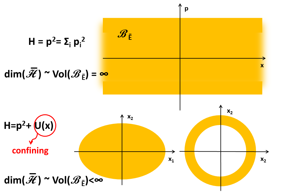
Figure 1: Up: Classically allowed phase space region $H(\bm{x}^{c},\bm{p}^{c})\leq\overline{E}$ if $H=\bm{p}^{2}$.  Down: Classically allowed configuration space region if $H=\bm{p}^{c}{}^{2}+V\big{(}\bm{x}^{c}\big{)}$, with the potential of the form $V\big{(}\bm{x}^{c}\big{)}=a(x_{1}^{c})^{2}+b(x_{2}^{c})^{2}$ (left) or $V\big{(}\bm{x}^{c}\big{)}=2k(r_{c}-1)^{2}$ (right), where $r_{c}=\sqrt{\bm{x}^{c}{}^{2}}$.

As a ${\cal T}$ consider now quantum mechanics (QM) of a zero spin particle on $\mathbb{R}^{D}$ with a Hamiltonian $H(\bm{x},\bm{p})$. If $\overline{{\cal H}}$ is the subspace with energies $E\leq\overline{E}$ then its dimension is approximately the phase space volume of the classical region ${\cal B}_{\scriptscriptstyle\overline{E}}$ determined by the inequality $H\big{(}\bm{x}^{c},\bm{p}^{c}\big{)}\leq\overline{E}$, in Planck constant units:

$$\mbox{dim}(\overline{{\cal H}})\simeq\mbox{Vol}({\cal B}_{\scriptscriptstyle\overline{E}})/h^{D}.$$

This is still infinite if e.g. $H$ reduces to the kinetic term $\bm{p}^{2}$ (upper part of fig. 1), while it is finite if $H$ contains a sufficiently strong binding potential $V(\bm{x})$ (lower part of fig. 1); consequently $\overline{{\cal T}}$ will be a fuzzy approximation of QM approximately confined in the (configuration space) region ${\cal R}\subset\mathbb{R}^{D}$ determined by the inequality $V(\bm{x})\leq\overline{E}$. We can obtain a NC, fuzzy approximation of QM on a submanifold $N$ of $\mathbb{R}^{D}$ adding a ‘dimensional reduction’ mechanism, more precisely a $V(\bm{x})$ with a sharp minimum on $N$.

In the rest of the paper we report on our application [1, 2, 3, 4, 5] of the mechanism for $N$ equal to the $d=(D\!-\!1)$-dimensional sphere $S^{d}$ of radius $r=1$ ($r^{2}:=\bm{x}^{2}$ is the square distance from the origin) and on the study of the resulting fuzzy spheres for $d=1,2$ [1, 2, 3, 4]; the lower right corner of fig. 1 shows the corresponding region ${\cal R}$ (a thin spherical shell of radius $\simeq 1$) in the $d=1$ case. The plan is as follows. Section 2 contains further preliminaries. In section 3 we sketch the construction procedure of $S^{d}_{\Lambda}$ for generic $d\geq 1$. In sections 4, 5 we respectively review the main features of $S^{1}_{\Lambda},S^{2}_{\Lambda}$, the eigenvalues and eigenvectors of the associated coordinate operators $x_{i}$ (for the latter we prove slightly stronger results than in [3]); then we present various systems of coherent states (SCS) on them and discuss their localization both in configuration and (angular) momentum space. Finally, in section 6 we draw the conclusions and add final remarks, while comparing our $S^{d}_{\Lambda}$ with other fuzzy spheres, in particular the celebrated Madore-Hoppe Fuzzy sphere (FS) [17, 18].

2 Further preliminaries

2.1 Covariance

$O(D)$-covariance of the theory means that for any orthogonal matrix $g\in O(D)$ there is a unitary transformation $U(g)$ of the Hilbert space ${\cal H}$ (or $\overline{{\cal H}}$) such that $g_{ij}v_{j}=U^{\dagger}\!(g)\,v_{i}\,U(g)$ for all vectors $\bm{v}$, and similarly for other $O(D)$-tensors. Fixed a $\bm{v}$, we can split

$${\cal H}=\bigcup_{\bm{u}\in S^{d}}{\cal H}_{\bm{u}},\qquad\qquad{\cal H}_{\bm{u}}:=\left\{\psi\in{\cal H}\>\>\>|\>\>\>\left\langle\bm{v}\right\rangle_{\psi}=\left|\langle\bm{v}\rangle_{\psi}\right|\,\bm{u}\,\right\}.$$ (1)

For each (unit vector) $\bm{u}\in S^{d}$ consider a $g\!\in\!O(D)$ such that $g\bm{u}\!=\!\bm{e}_{1}$, where $\bm{e}_{1}\!:=\!(1,\!0,\!...,\!0)$, and define  $\bm{v}^{\prime}\!:=\!g\bm{v}$,  so that $\bm{v}\cdot\bm{u}=v_{1}^{\prime}$. For all $\psi\in{\cal H}_{\bm{u}}$  we find  $\left\langle\bm{v}^{\prime}\right\rangle_{\psi}=|\langle\bm{v}\rangle_{\psi}|\bm{e}_{1}$;  moreover,  ${\cal H}_{\bm{u}}=U^{\dagger}(g){\cal H}_{\bm{e}_{1}}$ (of course one obtains the same result replacing $\bm{e}_{1}$ by any other $\bm{e}_{i}$).

2.2 Localization on $\mathbb{R}^{D}$, $S^{d}$ and $S^{d}_{\Lambda}$

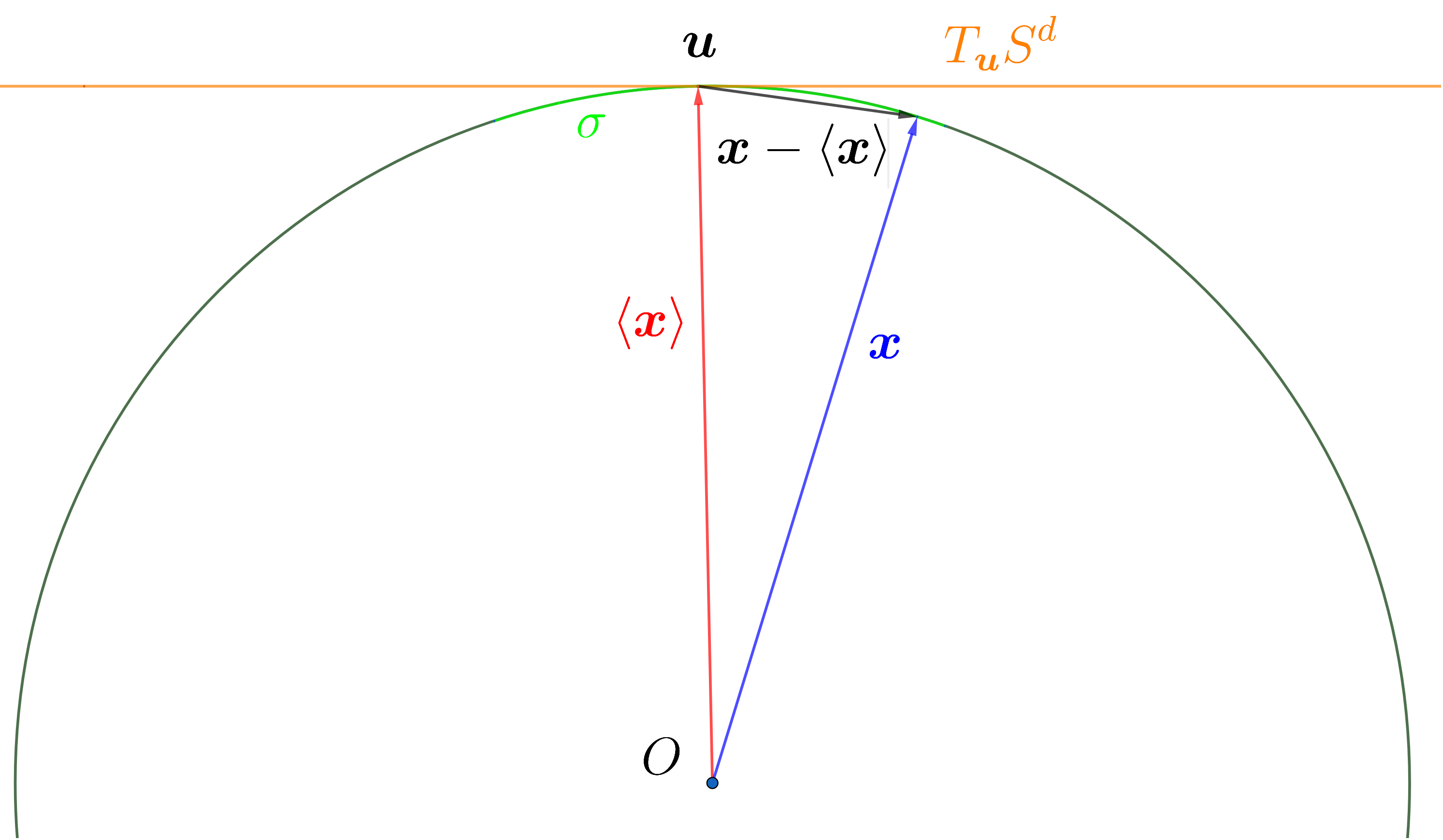
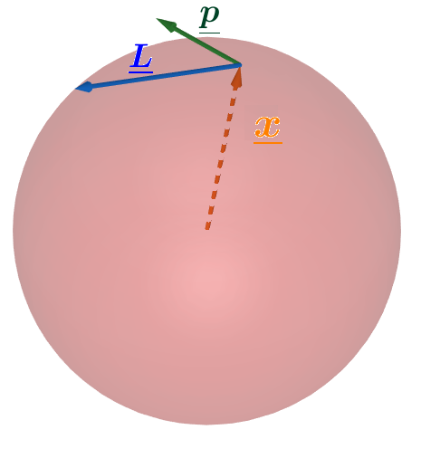
Figure 2: Left: the vectors $\bm{x}$, $\bm{u}\equiv\left\langle\bm{x}\right\rangle$, $\bm{x}-\left\langle\bm{x}\right\rangle$, the region $\sigma$ and the tangent plane $T_{\bm{u}}S^{d}$ at $\bm{u}$.  Right: perpendicularity of $\bm{x}$ and $\bm{L}$.

A good measure of the localization of a state in configuration space $\mathbb{R}^{D}$ is its spacial dispersion, i.e. the $O(D)$-invariant (and therefore reference-frame-independent) expectation value

$$(\Delta\bm{x})^{2}\equiv\sum_{i=1}^{D}(\Delta x_{i})^{2}\equiv\left\langle\left(\bm{x}\!-\!\left\langle\bm{x}\right\rangle\right)^{2}\right\rangle=\left\langle\bm{x}^{2}\right\rangle-\left\langle\bm{x}\right\rangle^{2}$$ (2)

on the state. Here $\bm{x}\equiv(x_{1},...,x_{n})$ is the vector position observable of the particle in the ambient Euclidean space $\mathbb{R}^{D}$, the vector $\left\langle\bm{x}\right\rangle\equiv(\left\langle x_{1}\right\rangle,...,\left\langle x_{n}\right\rangle)$ pinpoints the average position, the scalar observable $\bm{x}^{2}:=\sum_{i=1}^{D}x_{i}x_{i}$  measures the square distance from the origin, the vector observable $\bm{x}\!-\!\left\langle\bm{x}\right\rangle$ measures the displacement from $\left\langle\bm{x}\right\rangle$; (2) is the expectation value of the square of the latter. We adopt $(\Delta\bm{x})^{2}$ also on $S^{d},S^{d}_{\Lambda}$: in fact, if the state is localized in a small region $\sigma\subset S^{d}$ around a point $\bm{u}\equiv\left\langle\bm{x}\right\rangle\in S^{d}$ then $(\Delta\bm{x})^{2}$ essentially reduces to the average square displacement in the tangent plane at $\bm{u}$ (see fig. 2, left), as wished. If $\bm{x}^{2}\equiv 1$ on the whole Hilbert space ${\cal H}$ (this occurs strictly if ${\cal H}={\cal L}^{2}(S^{d})$ and also on Madore’s FS $S^{2}_{n}$, only approximately on our $S^{d}_{\Lambda}$), then $\left\langle\bm{x}^{2}\right\rangle$ is state-independent, and (2) is minimal on the states with maximal $\left\langle\bm{x}\right\rangle^{2}$. By (1) with $\bm{v}=\bm{x}$, in each ${\cal H}_{\bm{u}}$ $\left\langle\bm{x}\right\rangle^{2}$ is maximized on the eigenvector(s) $\psi$ of $x_{1}^{\prime}=\bm{x}\cdot\bm{u}$ with the highest (in absolute value) eigenvalue (the latter exists on the Madore’s FS, while on $S^{d}$ it exists as a generalized eigenvector).

2.3 Diagonalization of a coordinate  $x_{i}$ ,  and most localized states

For $x_{i}$ to approximate well and $O(D)$-covariantly a coordinate of a quantum particle forced to stay on the commutative sphere $S^{d}$, its spectrum $\Sigma_{x_{i}}$ should fulfill at least the following properties:

1. $\Sigma_{x_{i}}$ is the same for all $i=1,...,D$ and choices of the reference frame. In particular, it is invariant under inversion  $x_{i}\mapsto-x_{i}$.

2. In the commutative limit $\Sigma_{x_{i}}$ becomes uniformly dense in $[-1,1]$, in particular the maximal and the minimal eigenvalues converge to $1$ and $-1$, respectively.

These properties are fulfilled by both the Madore FS and (at least for $d=1,2$) our $S^{d}_{\Lambda}$. As explained in the previous subsection, the eigenstates with maximal eigenvalue (in absolute value) have also maximal localization on $S^{d},S^{2}_{n}$; this also approximately ture on our $S^{d}_{\Lambda}$.

2.4 Systems of coherent states (SCS)

We recall that the canonical SCS  $\{\phi_{z}\}_{z\in\Omega}\subset{\cal H}$ on $\mathbb{R}^{D}$ can be defined in three equivalent ways:

1. As the set of states saturating Heisenberg uncertainty relations (HUR)  $\Delta x_{i}\Delta p_{i}\geq 1/2$.

2. As the set of eigenstates of all annihilation operators $a_{i}$ with set of joint eigenvalues $z\in\Omega$.

3. As the set of states generated by the group $G$ acting on the vacuum state $\phi_{0}$.

Here ${\cal H}={\cal L}^{2}(\mathbb{R}^{D})$, $\Omega\!\equiv\!\mathbb{C}^{D}$, all variables have been made dimensionless, $a_{i}=x_{i}+ip_{i}$, and $G$ is the Heisenberg-Weyl group. Characterizations 1 (for $D=3$), 2, 3 are due to Schrödinger himself and Klauder, Sudarshan, Glauber [33, 34, 35, 36]. All of them admit (in general, non-equivalent) generalizations; see e.g. [37, 38, 39, 40, 41, 42], also for an overview on applications in elementary particle, nuclear, atomic, condensed matter, plasma physics. The canonical SCS fulfills the following properties:

1. Strong continuity of $\phi_{z}$ as a function of $z\in\Omega$;

2. Resolution of the identity: $\quad\mbox{id\,}=\int_{\Omega}\,d\!\mu(z)\>P_{z},\qquad P_{z}=\phi_{z}\langle\phi_{z},\cdot\rangle\equiv|\phi_{z}\rangle\langle\phi_{z}|;$

3. Completeness:   $\overline{\mbox{Span}\left\{\phi_{z}\>|\>z\in\Omega\right\}}=\mathcal{H}$.

where $d\mu(z)=d\Re(z)\,d\Im(z)$, and the resolution b) is in the weak sense. These properties are often used [37] for defining SCS in general: a set $\{\phi_{z}\}_{z\in\Omega}\subset{\cal H}$, where $\Omega$ is a topological label space, is a strong SCS if it fulfills a), b) with a suitable integration measure $d\!\mu(z)$ on $\Omega$; a weak SCS if it fulfills a), c).  As b) implies c), a strong SCS is also weak. Perelomov and Gilmore develop [30, 32] the concept of SCS through approach 3 choosing $\Omega$ either a generic Lie group $G$, or more generally a coset $G/H$ thereof, acting on ${\cal H}$ via an irreducible unitary representation $T$ (see e.g. [31]). The steps are as follows:

• For all   $\phi_{0}\!\in\!{\cal H}$,  let  $\phi_{g}\!\equiv\!T(g)\phi_{0}$ for all $g\!\in\!G$,  $H\!\equiv\!\{h\!\in\!G\>\>|\>\>\phi_{h}=\exp{\left[i\alpha(h)\right]}\phi_{0}\}$.

• Then  $|\phi_{g}\rangle\langle\phi_{g}|=|\phi_{gh}\rangle\langle\phi_{gh}|\equiv P_{z}$,  i.e. depends only on  $z\equiv[g]\in G/H\equiv\Omega$.

• If $\phi_{0}$ is admissible, i.e. $\int_{G}|\langle\phi_{0},\!T(g)\phi_{0}\rangle|^{2}\,dg<\infty$, where $dg$ is the left-invariant Haar measure on $G$, then b) holds with $d\!\mu(z)$ the normalized measure induced by $dg$ on $\Omega$.

Clearly, if $G$ is compact all $\phi_{0}\!\in\!{\cal H}$ are admissible. Following Perelomov, the CS that are closest to classical states are obtained from a $\phi_{0}$ that maximizes $H$, or better the isotropy subalgebra $\mathfrak{b}$ in the complex hull of the Lie algebra of $G$; $\phi_{0}$ is annihilated by some element(s) in $\mathfrak{b}$, the corresponding $\phi_{g}$ are eigenvectors of the latter (property 2) and minimize the $G$-invariant uncertainty associated to the quadratic Casimir [$(\Delta\bm{L})^{2}=\sum_{i<j}\Delta L_{ij}^{2}$ in the case $G=SO(D)$]. For $G=SO(3)$ it is $H=SO(2)$, $(\Delta\bm{L})^{2}=\left\langle\bm{L}^{2}\right\rangle-\left\langle\bm{L}\right\rangle^{2}$ (with  $L_{i}\equiv\varepsilon^{ijk}L_{jk}/2$),  and minimizing $(\Delta\bm{L})^{2}$ amounts to saturating a specific UR [4] (hence also property 1 holds); this SCS consists of the socalled coherent spin or Bloch states.

In introducing SCS on $S^{d}_{\Lambda}$ ($d=1,2$) we follow in spirit Perelomov’s approach, with $G$ the isometry group $O(D)$ of $S^{d}$ (a compact group). However, our Hilbert space $\mathcal{H}_{\Lambda}$ will in general carry a reducible representation of $O(D)$; moreover, we study the localization properties of these SCS both in configuration and (angular) momentum space.

3 Construction of the $S^{d}_{\Lambda}$ for general $d\geq 1$

Figure 3: Three-dimensional plot of $V(r)$

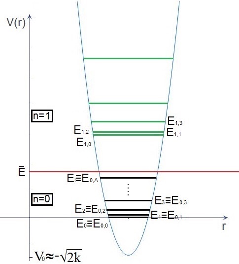
Figure 4: Two-dimensional plot of $V(r)$ including the energy-cutoff and allowed energy levels (black).

The main steps of the costructions are as follows:

• We adopt a $O(D)$ invariant Hamiltonian

  $$H=-\frac{1}{2}\Delta+V(r),$$ (3)

  where the confining potential $V(r)$ has a very sharp minimum $V_{0}=V(1)$ at $r=1$. More precisely, we assume that

  $$V(r)\simeq V_{0}+2k\left(r\!-\!1\right)^{2}\qquad\mbox{if }V(r)\leq\overline{E},$$ (4)

  so that $V(r)$ has a harmonic behavior for  $\left|r\!-\!1\right|\!\leq\!\sqrt{\!\frac{\overline{E}\!-\!V_{0}}{2k}}$, and that $V^{\prime\prime}(1)\!\equiv\!4k\!\gg\!0$ ($k$ thus parametrizes the sharpness of the minimum); we fix $V_{0}$ so that the ground state has energy $E_{0}=0$. Using polar coordinates we can decompose $\Delta=\partial_{r}^{2}+\frac{d}{r}\partial_{r}-\frac{1}{r^{2}}\bm{L}^{2}$, where $\bm{L}^{2}:=L_{ij}L_{ij}/2$ is the square angular momentum [$L_{ij}:=i(x_{j}\frac{\partial}{\partial x_{i}}\!-\!x_{i}\frac{\partial}{\partial x_{j}})$ are the angular momentum components], i.e. the Hamiltonian of free motions (the Laplacian) on $S^{d}$. Looking for the eigenfunctions $\psi$ of $H$ in the form $\psi=f(r)Y(\varphi,...)$, where $\varphi,...$ are the angular coordinates, we reduce the eigenvalue equation $H\psi=E\psi$ to a 1-dimensional Schrödinger equation in the form of an ordinary differential equation with respect to $r$. The eigenvalues are parametrized by integers $l,n\geq 0$; they respectively determine the eigenvalue  $E_{l}\equiv l(l\!+\!d\!-\!1)$  of $\bm{L}^{2}$ and the radial excitation, which at least for small $n$ are approximately of harmonic type,  $\simeq\sqrt{8}kn$.

• We choose $\overline{E}$ low enough, e.g. $\overline{E}\lesssim\sqrt{8}k$, to constrain $n$ to be zero, namely to eliminate radial excitations from the spectrum $\Sigma_{\overline{H}}$ of $\overline{H}$, so that the latter reduces to that of $\overline{\bm{L}^{2}}$,   $\Sigma_{\overline{H}}=\{E_{l}\}$. Then we also find that the $x_{i}$ generate the whole algebra of observables $\overline{{\cal A}}$, and   $[\overline{x_{i}},\overline{x_{j}}]\simeq-iL_{ij}/k$,  i.e. we find Snyder-type commutation relations among the coordinates. There is a residual freedom in the choice of $V(r)$ (the higher order terms in the Taylor expansion of $V(r)$ around $r=1$); we fine-tune the model requiring that $[\overline{x_{i}},\overline{x_{j}}]=-iL_{ij}/k$ (up to terms that act non-trivially only on the highest energy states).

• To obtain a sequence of finite-dimensional models going to QM on $S^{d}$ we make $\overline{E}$ grow and diverge with a natural number $\Lambda$; so must also $k$ do, in order that the above inequality keeps holding. We choose  $\overline{E}\equiv E_{\Lambda}=\Lambda(\Lambda\!+\!d\!-\!1)$ and $V$ depending on $\Lambda$ so that $k(\Lambda)\geq\Lambda^{2}(\Lambda\!+\!1)^{2}$;  correspondingly, $\Sigma_{\overline{H}}=\{E_{l}\}_{l=1}^{\Lambda}$, and replacing everywhere the bar by the subscript $\Lambda$ we find

  $$({\cal H}_{\Lambda},{\cal A}_{\Lambda})\stackrel{{\scriptstyle\Lambda\to\infty}}{{\longrightarrow}}\left({\cal H},{\cal A}\right)\equiv\left({\cal L}^{2}(S^{d}),\,\mbox{Lin}\!\left({\cal L}^{2}(S^{d})\right)\right)$$ (6)

  in a suitable sense [1]. $\{S^{d}_{\Lambda}\}_{\Lambda\in\mathbb{N}}\equiv\{({\cal H}_{\Lambda},{\cal A}_{\Lambda})\}_{\Lambda\in\mathbb{N}}$ is our $d$-dimensional, $O(D)$-covariant fuzzy sphere, i.e. a sequence of finite-dimensional approximations of ordinary QM on $S^{d}$.

It turns out that (at least for $D=2,3$) there exist $O(D)$-covariant $*$-algebra isomorphisms  ${\cal A}_{\Lambda}\simeq\pi_{\Lambda}[Uso(D+1)]$,  where $(\pi_{\Lambda},{\cal H}_{\Lambda})$ is a suitable irreducible unitary representation of $Uso(D+1)$. More precisely, in terms of the canonical basis  $\{{\sf L}_{IJ}\,|\,1\leq I<J\leq D\!+\!1\}$  of $so(D+1)$,

$$\overline{L_{ij}}=\pi_{\Lambda}({\sf L}_{ij}),\qquad\overline{x_{h}}=\pi_{\Lambda}\left[f_{1}\!\left(\bm{L}^{2}\right)\,{\sf L}_{h({D+1})}\,f_{2}\!\left(\bm{L}^{2}\right)\right],\qquad 1\leq i,j,h\leq D,\quad i<j,$$ (7)

where and $f_{1}(s),f_{2}(s)$ are suitable analytic functions.

To simplify the notation, below we shall remove the bar and denote the generic $\overline{A}\in\mathcal{A}_{\Lambda}$ as $A$.

4 $D=2$: $O\left(2\right)$-covariant fuzzy circle

In a suitable orthonormal basis ${\cal B}_{\Lambda}:=\{\psi_{\Lambda},\psi_{\Lambda-1},...,\psi_{-\Lambda}\}$ of the Hilbert space ${\cal H}_{\Lambda}$ consisting of eigenvectors of the angular momentum $L\equiv L_{12}$,

$$L\,\psi_{n}=n\,\psi_{n},$$ (8)

the action of the noncommutative coordinates  $x_{\pm}:=x_{1}\pm ix_{2}$  of the fuzzy circle $S^{1}_{\Lambda}$ read

$$x_{\pm}\,\psi_{n}\>=\>\left\{\begin{array}[]{ll}\!\!\displaystyle\left[1\!+\!\frac{n(n\pm 1)}{2k}\right]\psi_{n\pm 1}&\mbox{if }-\!{{\Lambda}}\leq\pm n\leq{{\Lambda}}\!-\!1,\\[8.0pt] 0&\mbox{otherwise,}\end{array}\right.$$ (11)

where $k=k(\Lambda)\geq\Lambda^{2}(\Lambda\!+\!1)^{2}$. In the $\Lambda=\infty$ limit $x_{\pm}=e^{\pm i\varphi}$, $\psi_{n}=e^{in\varphi}$ (up to a phase); $\varphi$ is the angle along $S^{1}$. $L,x_{+},x_{-}$ and $\bm{x}^{2}:=x_{1}^{2}+x_{2}^{2}=\frac{1}{2}(x_{+}x_{-}+x_{-}x_{+})$ fulfill the $O(2)$-equivariant relations

$$\left[L,x_{\pm}\right]=\pm x_{\pm},\quad x_{+}{}^{\dagger}=x_{-},\qquad L^{\dagger}=L,$$ (12)

$$\left[x_{+},x_{-}\right]={\color[rgb]{1,0,0}{-\frac{2L}{k}+\left[1\!+\!\frac{\Lambda(\Lambda\!+\!1)}{k}\right]\!\left(\widetilde{P}_{\Lambda}\!-\!\widetilde{P}_{-\Lambda}\right)\equiv L^{\prime}}},$$ (13)

$$\bm{x}^{2}=1\>{\color[rgb]{1,0,0}{+\frac{L^{2}}{k}-\left[1\!+\!\frac{\Lambda(\Lambda\!+\!1)}{k}\right]\frac{\widetilde{P}_{\Lambda}\!+\!\widetilde{P}_{-\Lambda}}{2}}},$$ (14)

$$\prod\limits_{n=-\Lambda}^{\Lambda}\!\!\left(L\!-\!n\,I\right)=0,\qquad\left(x_{\pm}\right)^{2\Lambda+1}=0.$$ (15)

Here $\widetilde{P}_{n}$ is the projection onto the $1$-dim subspace $\mathbb{C}\psi_{n}$. Terms marked red are absent in the commutative case. In the $\Lambda\to\infty$ limit also the non-vanishing ones will play no role at any fixed energy $E$, as they are proportional to the projections $\widetilde{P}_{\pm\Lambda}$ onto the states with highest energy $E_{\Lambda}\to\infty$; (15a) gives back $\Sigma_{L}=\mathbb{Z}$, whereas (15b) looses meaning and must be dropped. We point out that:

• $\bm{x}^{2}\neq 1$, but it is a function of $L^{2}$, hence the $\psi_{n}$ are its eigenvectors; its eigenvalues (except on $\psi_{\pm\Lambda}$) are close to 1, slightly grow with $|n|$ and collapse to 1 as $\Lambda\to\infty$.

• The ordered monomials $x_{+}^{h}\,L^{l}\,x_{-}^{n}$ [with degrees $h,l,n$ bounded by (12)-15] make up a basis of the $(2\Lambda\!+\!1)^{2}$-dim vector space underlying the algebra of observables  ${\cal A}_{\Lambda}\!:=\!End({\cal H}_{\Lambda}\!)$  (the $\widetilde{P}_{n}$ themselves can be expressed as polynomials in $L$).

• $x_{+},x_{-}$ generate the whole $*$-algebra ${\cal A}_{\Lambda}$, because also $L$ can be expressed as a non-ordered polynomial in $x_{+},x_{-}$.

• As anticipated in (7), actually there are $O(2)$-equivariant $*$-algebra isomorphisms ${\cal A}_{\Lambda}$

  $${\cal A}_{\Lambda}\simeq M_{N}(\mathbb{C})\simeq\pi_{\Lambda}[Uso(3)],\qquad N=2\Lambda\!+\!1,$$ (16)

  where $\pi_{\Lambda}$ is the $N$-dimensional unitary irreducible representation of $Uso(3)$. The latter is characterized by the condition $\pi_{\Lambda}(C)=\Lambda(\Lambda+1)$, where $C=E_{a}E_{-a}$ is the Casimir (sum over $a\in\{+,0,-\}$), and $E_{a}$ make up the Cartan-Weyl basis of $so(3)$,

  $$[E_{+},E_{-}]=E_{0},\qquad[E_{0},E_{\pm}]=\pm E_{\pm},\qquad E_{a}^{\dagger}=E_{-a}.$$ (17)

  In fact we can realize   $L,x_{+},x_{-}$  by setting [1] (we simplify the notation dropping $\pi_{{{\Lambda}}}$)

  $$\begin{array}[]{c}L=E_{0},\qquad x_{\pm}=f_{\pm}(E_{0})E_{\pm},\\[10.0pt] \displaystyle f_{+}(s)=\sqrt{\frac{1\!+\!s(s\!-\!1)/k}{{{\Lambda}}({{\Lambda}}+1)\!-\!s(s\!-\!1)}}=f_{-}(s-1),\end{array}\$$ (18)

  i.e. in a sense the $x_{\pm}$ are $E_{\pm}$ (which play the role of $x_{\pm}$ in Madore FS) squeezed in the $E_{0}$ direction; one can easily check (12-15) using (26), with $L_{a},l,m$ resp. replaced by $E_{a},\Lambda,n$. Hence  $\pi_{\Lambda}(E_{+}),\pi_{\Lambda}(E_{-})$   are generators of ${\cal A}_{\Lambda}$ alternative to  $x_{+},x_{-}$.

• The group $Y_{\Lambda}\simeq SU(2\Lambda\!+\!1)$ of $*$-automorphisms of ${\cal A}_{\Lambda}$ is inner and includes a subgroup $SO(3)$ independent of $\Lambda$ (acting irreducibly via $\pi_{\Lambda}$) and a subgroup $O(2)\subset SO(3)$ corresponding to orthogonal transformations (in particular, rotations) of the coordinates $x_{i}$, which plays the role of isometry group of $S^{1}_{\Lambda}$.

As in the commutative case we define  $\left\langle\bm{x}\,\right\rangle^{2}\!:=\!\langle x_{1}\rangle^{2}\!+\!\langle x_{2}\rangle^{2}$ and find $\left\langle\bm{x}\,\right\rangle^{2}\!=\!\langle x_{+}\rangle\langle x_{-}\rangle\!=\!|\langle x_{+}\rangle|^{2}$.

4.1 Diagonalization of the coordinates $x_{i}$ on $S^{1}_{\Lambda}$

As said, by $O(2)$-covariance $\Sigma_{x_{i}}\left(\Lambda\right)=\Sigma_{x_{1}}\left(\Lambda\right)$ for all $i$, so we can study just the spectrum $\Sigma_{x_{1}}\left(\Lambda\right)$. $L$ is invariant under $2$-dimensional rotations, whereas $L\to-L$ under $x_{1}$- or $x_{2}$-inversion. On the basis ${\cal B}_{\Lambda}$ the operator $x_{1}$ is represented by the $(2\Lambda\!+\!1)\times(2\Lambda\!+\!1)$ symmetric tridiagonal matrix

$$X(\Lambda)=\frac{1}{2}\left(\begin{array}[]{cccccccc}0&b_{\Lambda}&0&0&\dots&0&0&0\\ b_{\Lambda}&0&b_{\Lambda-1}&0&\dots&0&0&0\\ 0&b_{\Lambda-1}&0&b_{\Lambda-2}&\dots&0&0&0\\ \vdots&\vdots&\vdots&\vdots&\ddots&\vdots&\vdots&\vdots\\ \vdots&\vdots&\vdots&\vdots&\ddots&\vdots&\vdots&\vdots\\ \vdots&\vdots&\vdots&\vdots&\ddots&\vdots&\vdots&\vdots\\ 0&0&0&0&\cdots&b_{2-\Lambda}&0&b_{1-\Lambda}\\ 0&0&0&0&\cdots&0&b_{1-\Lambda}&0\end{array}\right)=X^{0}(\Lambda)+O\!\left(\!\frac{1}{\Lambda^{2}}\!\right).$$

Here $b_{n}\equiv\sqrt{1\!+\!n(n\!-\!1)/k}$,  and $X^{0}$ is the $k\to\infty$ limit of $X$, i.e. is obtained replacing all $b_{n}$ by $1$. The eigenvectors and eigenvalues of Toeplitz matrices such as $X^{0}$ are known (see e.g. [47] p. 2-3) and are good approximations of those of $x_{1}$; in [3] we have studied the latter estimating the needed corrections. The spectrum of $X^{0}(\Lambda)$ arranged in descending order is  $\Sigma_{X_{0}}:=\left\{\widetilde{\alpha}_{h}(\Lambda)\right\}_{h=1}^{N}$,  where

$$\widetilde{\alpha}_{h}=\cos{\left(\frac{h\pi}{N+1}\right)},$$ (19)

and $N=2\Lambda+1$. We shall arrange also the spectrum $\Sigma_{X(\Lambda)}=\left\{\alpha_{h}(\Lambda)\right\}_{h=1}^{2\Lambda+1}$ of $x_{1}\simeq X$ in decreasing order. Improving the results of Theorem 3.1 in [3], here we prove

Theorem 4.1.

For all $\Lambda\in\mathbb{N}$

1. If $\alpha$ belongs to $\Sigma_{X}$, then also $-\alpha$ does.

2. $\Sigma_{X(\Lambda)},\Sigma_{X(\Lambda+1)}$ interlace, i.e. between any two consecutive eigenvalues of $X(\Lambda\!+\!1)$ there is exactly one of $X(\Lambda)$ (see fig. 5):

   $$\alpha_{1}\left(\Lambda\!+\!1\right)\>>\>\alpha_{1}\left(\Lambda\right)\>>\>\alpha_{2}\left(\Lambda\!+\!1\right)\>>\>\alpha_{2}\left(\Lambda\right)\>>...\>>\>\alpha_{\Lambda}\left(\Lambda\right)\>>\>\alpha_{\Lambda+1}\left(\Lambda\!+\!1\right);$$

3. $\Sigma_{X}$ becomes uniformly dense in $[-1,1]$ as $\Lambda\to\infty$, in particular  $\displaystyle\alpha_{1}\left(\Lambda\right)\geq 1-\frac{\pi^{2}}{8(\Lambda+1)^{2}}$.

Proof.

Items 1., 3. were proved in Theorem 3.1 in [3]. Item 1. follows also from Proposition 7.1, after the inversion $X_{m}\mapsto-X_{m}$. We prove item 2.with the help of Proposition 7.1 (?) COMPLETARE. ∎

Note that item 2. implies in particular that all eigenvalues are simple.

In the $\Lambda\to\infty$ the eigenvectors of $x_{1}$ become generalized eigenvectors, as expected.

4.2 $O(2)$-covariant uncertainty relations and $O(2)$-invariant strong SCS systems

From (12) one can derive [4] for both $S^{1},S^{1}_{\Lambda}$ the $O(2)$-covariant ‘Heisenberg’ uncertainty relations

$$\Delta L\,\Delta x_{1}\geq\frac{|\langle x_{2}\rangle|}{2},\qquad\Delta L\,\Delta x_{2}\geq\frac{|\langle x_{1}\rangle|}{2},\qquad\Delta L^{2}(\Delta\bm{x})^{2}\geq\frac{\langle\bm{x}\rangle^{2}}{4};$$ (20)

they are saturated by the $\psi_{n}$ ($\Delta L=0$). We have also shown that $\Delta x_{1},\Delta x_{2}$ may vanish separately, but not simultaneously, because

$$(\Delta\bm{x})^{2}\geq(\Delta\bm{x})^{2}_{min}\sim{\color[rgb]{1,0,0}{\frac{1}{\Lambda^{2}}}}.$$ (21)

Theorem (section 3.1 in [4])  The system  ${\cal S}^{\beta}\equiv\left\{{\bm{\omega}}_{\alpha}^{\beta}\equiv\!\!\sum\limits_{n=-\Lambda}^{\Lambda}\!\!\frac{e^{i(\alpha n+\beta_{n})}}{\sqrt{2\Lambda\!+\!1}}\psi_{n}\right\}_{\!\!\alpha\in\mathbb{R}/2\pi\mathbb{Z}}$ is a strong SCS,

$$\frac{2\Lambda\!+\!1}{2\pi}\int_{0}^{2\pi}\!\!\!\!d\alpha\,P^{\beta}_{\alpha}=\mbox{id\,},\qquad P_{\alpha}^{\beta}\equiv{\bm{\omega}}_{\alpha}^{\beta}\langle{\bm{\omega}}_{\alpha}^{\beta},\cdot\rangle,\qquad$$ (22)

for all $\beta\in(\mathbb{R}/2\pi\mathbb{Z})^{2\Lambda\!+\!1}$ (the label space is $\mathbb{R}/2\pi\mathbb{Z}\simeq S^{1}\equiv\Omega$). It is fully $O(2)$-covariant if $\beta_{-n}=\beta_{n}$.  On all ${\bm{\omega}}_{\alpha}^{\beta}$ it is $\langle L\rangle=0$, $\left(\Delta L\right)^{2}=\frac{\Lambda(\Lambda\!+\!1)}{3}$, whereas $(\Delta\bm{x})^{2}$ is minimized by the ${\bm{\phi}}_{\alpha}\equiv{\bm{\omega}}_{\alpha}^{0}$, with

$$\left(\Delta\bm{x}\right)^{2}<\frac{1}{\Lambda+1}\left(\frac{1}{2}+\frac{1}{3\Lambda}\right).$$ (23)

Within the class of strong SCS, the ${\bm{\phi}}_{\alpha}$ are closest to classical states(=points) of $S^{1}$, and in one-to-one correspondence with them:  $S^{1}\leftrightarrow{\cal S}^{1}\equiv\{{\bm{\phi}}_{\alpha}\}_{\alpha\in\mathbb{R}/2\pi\mathbb{Z}\simeq S^{1}\equiv\Omega}$.

4.3 $O(2)$-invariant weak SCS minimizing $(\Delta\bm{x})^{2}$

Since $(\Delta\bm{x})^{2}$ is $O(2)$-invariant, so is the set ${\cal W}^{1}$ of states minimizing it; ${\cal W}^{1}$ is a weak SCS. We can recover the whole set from any element $\underline{\bm{\chi}}$ through rotations,  ${\cal W}^{1}=\left\{\underline{\bm{\chi}}_{\alpha}\!\equiv e^{i\alpha L}\underline{\bm{\chi}}\right\}_{\!\alpha\in[0,2\pi[}$. Choosing $\underline{\bm{\chi}}$ so that $\langle x_{2}\rangle_{\underline{\bm{\chi}}}=0$, by (1) we find $\langle\bm{x}\rangle_{\underline{\bm{\chi}}_{\alpha}}=\left|\langle\bm{x}\rangle_{\underline{\bm{\chi}}}\right|\bm{u}_{\alpha}$, where $\bm{u}_{\alpha}=(\cos\alpha,\sin\alpha)$. We have shown that

$$0<\left(\Delta{\bm{x}}\right)^{2}_{min}=\left(\Delta{\bm{x}}\right)^{2}_{\underline{\bm{\chi}}_{\alpha}}<\frac{3.5}{(\Lambda+1)^{2}}.$$ (24)

The (rays associated to) $\underline{\bm{\chi}}_{\alpha}$ are closest to classical states(=points) of $S^{1}$, and in one-to-one correspondence with them:  $S^{1}\leftrightarrow{\cal S}^{1}\equiv\{{\bm{\phi}}_{\alpha}\}_{\alpha\in\mathbb{R}/2\pi\mathbb{Z}\simeq S^{1}}$.

5 D=3:$O\left(3\right)$-covariant fuzzy sphere

We use two related sets of angular momentum and space coordinate operators: the hermitean ones  $\left\{L_{i}\right\}_{i=1}^{3}$ (with $L_{i}\equiv\varepsilon^{ijk}L_{jk}/2$)  and $\left\{x_{i}\right\}_{i=1}^{3}$, and the partly hermitean conjugate ones  $\left\{L_{a}\right\}$, $\left\{x_{a}\right\}$ (here $a=0,+,-$),  which are obtained from the former as follows:

$$L_{\pm}:=L_{1}\pm iL_{2},\quad\quad L_{0}:=L_{3},\quad\quad x_{\pm}:=x_{1}\pm ix_{2},\quad\quad x_{0}:=x_{3}.$$

The square distance from the origin can be expressed as $\bm{x}^{2}:=x_{i}x_{i}=x_{0}^{2}+(x_{+}x_{-}+x_{-}x_{+})/2$. As a preferred orthonormal basis of the carrier Hilbert space ${\cal H}_{\Lambda}$ we adopt one ${\cal B}_{\Lambda}$ consisting of eigenvectors of  $L_{3}$,   $\bm{L}^{2}=L_{i}L_{i}=L_{0}^{2}+(L_{+}L_{-}+L_{-}L_{+})/2$,

$${\cal B}_{\Lambda}:=\left\{\psi_{l}^{m}\right\}_{l=0,1,...,\Lambda;\ m=-l,...,l},\qquad\bm{L}^{2}\psi_{l}^{m}=l(l+1)\psi_{l}^{m},\qquad L_{3}\psi_{l}^{m}=m\psi_{l}^{m}.$$ (25)

On the $\psi_{l}^{m}$ the $L_{a},x_{a}$ act as follows:

$$L_{0}\psi_{l}^{m}=m\,\psi_{l}^{m},\quad L_{\pm}\psi_{l}^{m}=\sqrt{(l\!\mp\!m)(l\!\pm\!m\!+\!1)}\psi_{l}^{m\pm 1}\!,$$ (26)

$$x_{a}\psi_{l}^{m}=\left\{\!\!\begin{array}[]{ll}c_{l}A_{l}^{a,m}\psi_{l-1}^{m+a}+c_{l+1}B_{l}^{a,m}\psi_{l+1}^{m+a}&\mbox{ if }l<\Lambda,\\[8.0pt] c_{l}A_{l}^{a,m}\psi_{\Lambda-1}^{m+a}&\mbox{ if }l=\Lambda,\\[8.0pt] 0&\mbox{otherwise,}\end{array}\right.$$ (30)

where

$$\begin{array}[]{l}\displaystyle A_{l}^{0,m}:=\sqrt{\frac{(l+m)(l-m)}{(2l+1)(2l-1)}}\hskip 2.84544pt,\hskip 28.45274ptA_{l}^{\pm,m}:=\pm\sqrt{\frac{(l\mp m)(l\mp m-1)}{(2l-1)(2l+1)}}\hskip 2.84544pt,\\ \displaystyle B_{l}^{a,m}=A_{l+1}^{-a,m+a},\hskip 22.76228ptc_{l}:=\sqrt{1+\frac{l^{2}}{k}}\quad 1\leq l\leq\Lambda,\hskip 17.07182ptc_{0}=c_{\Lambda+1}=0\hskip 2.84544pt,\end{array}$$ (33)

and $k(\Lambda)$ fulfills $k(\Lambda)\geq\Lambda^{2}(\Lambda\!+\!1)^{2}$. The $L_{i},x_{i}$ fulfill the following $O(3)$-covariant relations:

$$x_{i}^{{\dagger}}=x_{i},\qquad L_{i}^{{\dagger}}=L_{i},\qquad[L_{i},x_{j}]=i\varepsilon^{ijh}x_{h},\qquad\left[\,L_{i},L_{j}\right]=i\varepsilon^{ijh}L_{h},\qquad x_{i}L_{i}=0,$$ (34)

$$[x_{i},x_{j}]={\color[rgb]{1,0,0}\underbrace{i\varepsilon^{ijh}L_{h}\left(\!\!-\!\frac{1}{k}\!+\!K\widetilde{P}_{\Lambda}\!\right)}_{Snyder-like}},\hskip 31.2982pt\bm{x}^{2}=1\>{\color[rgb]{1,0,0}{+\frac{\bm{L}^{2}\!+\!1}{k}-\left[1+\frac{(\Lambda\!+\!1)^{2}}{k}\right]\!\frac{\Lambda\!+\!1}{2\Lambda\!+\!1}\widetilde{P}_{\Lambda}}},$$ (35)

$$\prod_{l=0}^{\Lambda}\left[\bm{L}^{2}-l(l+1)I\right]=0,\hskip 42.67912pt\prod_{m=-l}^{l}{\left(L_{3}-mI\right)}\widetilde{P}_{l}=0,\hskip 42.67912pt\left(x_{\pm}\right)^{2\Lambda+1}=0;$$ (36)

here $K=\frac{1}{k}+\frac{1+\frac{\Lambda^{2}}{k}}{2\Lambda+1}$, $\widetilde{P}_{l}$ is the projection on the $\bm{L}^{2}=l(l+1)$ eigenspace. Again, terms marked red are absent in the commutative case. In the $\Lambda\to\infty$ limit also the non-vanishing ones will play no role at any fixed energy $E$, as they are proportional to the projection $\widetilde{P}_{\Lambda}$ onto the states with highest energy $E_{\Lambda}\to\infty$; (36a,b) give back the spectra of $\bm{L}^{2},L_{3}$ on ${\cal L}^{2}(S^{2}),{\cal L}^{2}(\mathbb{R}^{3})$, whereas (36c) looses meaning and must be dropped. We point out that:

• $\bm{x}^{2}\neq 1$; but it is a function of $\bm{L}^{2}$, hence the $\psi_{l}^{m}$ are its eigenvectors; its eigenvalues (except when $l=\Lambda$) are close to 1, slightly grow with $l$ and collapse to 1 as $\Lambda\to\infty$.

• The ordered monomials in $x_{i},L_{i}$ [with degrees bounded by (34-36)] make up a basis of the $(\Lambda\!+\!1)^{4}$-dim vector space  $\mathcal{A}_{\Lambda}\!:=\!End({\cal H}_{\Lambda}\!)\!\simeq\!M_{(\Lambda+1)^{2}}(\mathbb{C})$, because the $\widetilde{P}_{l}$ themselves can be expressed as polynomials in $\bm{L}^{2}$.

• The $x_{i}$ generate the $*$-algebra $\mathcal{A}_{\Lambda}$, because also the $L_{i}$ can be expressed as non-ordered polynomials in the $x_{i}$.

• As anticipated in (7), actually there are $O(3)$-covariant $*$-algebra isomorphisms

  $${\cal A}_{\Lambda}\simeq M_{N}(\mathbb{C})\simeq{\bm{\pi}}_{\Lambda}[Uso(4)],\quad N:=(\Lambda\!+\!1)^{2}.$$ (37)

  where ${\bm{\pi}}_{\Lambda}$ is the $N$-dimensional unitary vector (and irreducible) representation of $Uso(4)$ on the Hilbert space ${\bf V}_{\Lambda}$ characterized by the conditions ${\bm{\pi}}_{\Lambda}(C)=\Lambda(\Lambda+2)$, ${\bm{\pi}}_{\Lambda}(C^{\prime})=0$ on the quadratic Casimirs. In terms of the Cartan-Weyl basis $\{{\sf L}_{HI}\}$ ($H,I\in\{1,2,3,4\}$) of $so(4)$,

  $$\left[{\sf L}_{HI},{\sf L}_{JK}\right]=i\left(\delta_{HJ}{\sf L}_{IK}-\delta_{HK}{\sf L}_{IJ}-\delta_{IJ}{\sf L}_{HK}+\delta_{IK}{\sf L}_{HJ}\right),\qquad{\sf L}_{HI}^{\dagger}={\sf L}_{HI}=-{\sf L}_{IH},$$ (38)

  $C={\sf L}_{IJ}{\sf L}_{IJ}$, $C^{\prime}=\varepsilon^{HIJK}{\sf L}_{HI}{\sf L}_{JK}$ (sum over repeated indices). To simplify the notation we drop ${\bm{\pi}}_{\Lambda}$. In fact one can realize   $L_{i}\,,x_{i}$,  $i\in\{1,2,3\}$, by  setting [1]

  $$\begin{array}[]{rcl}L_{i}&=&\displaystyle\frac{1}{2}\varepsilon^{ijk4}{\sf L}_{jk},\qquad\qquad x_{i}=g^{*}(\lambda)\,{\sf L}_{4i}\,g(\lambda),\\[10.0pt] g(l)&=&\displaystyle\sqrt{\frac{\Gamma\!\left(\frac{\Lambda\!+\!l}{2}\!+\!1\right)\Gamma\!\left(\frac{\Lambda\!-\!l\!+\!1}{2}\right)}{\Gamma\!\left(\frac{\Lambda\!+\!1\!+\!l}{2}\!+\!1\right)\Gamma\!\left(\frac{\Lambda\!-\!l}{2}\!+\!1\right)}\frac{\Gamma\!\left(\frac{l}{2}\!+\!1\!+\!\frac{i\sqrt{k}}{2}\right)\Gamma\!\left(\frac{l}{2}\!+\!1\!-\!\frac{i\sqrt{k}}{2}\right)}{\sqrt{k}\>\Gamma\!\left(\frac{l\!+\!1}{2}\!+\!\frac{i\sqrt{k}}{2}\right)\Gamma\!\left(\frac{l\!+\!1}{2}\!-\!\frac{i\sqrt{k}}{2}\right)}}\\[22.0pt] &=&\displaystyle\sqrt{\frac{\prod_{h=0}^{l-1}(\Lambda\!+\!l\!-\!2h)}{\prod_{h=0}^{l}(\Lambda\!+\!l\!+\!1\!-\!2h)}\prod_{j=0}^{\left[\frac{l\!-\!1}{2}\right]}\frac{1+\frac{(l\!-\!2j)^{2}}{k}}{1+\frac{(l\!-\!1\!-\!2j)^{2}}{k}}}\>\>;\end{array}$$ (39)

  here we have introduced the operator $\lambda:=[\sqrt{4L_{i}L_{i}+1}-1]/2$ (which has eigenvalues $l\in\{0,1,...,\Lambda\}$), $\Gamma$ is Euler gamma function, the last equality holds only if $l\in\mathbb{N}_{0}$, and $[b]$ stands for the integer part of $b$. Therefore the $L_{HI}$ in the ${\bm{\pi}}_{\Lambda}$-representation make up also an alternative set of generators of ${\cal A}_{\Lambda}$ (in [1] ${\sf L}_{4i}$ is denoted by $X_{i}$).

• The group $Y_{\Lambda}\simeq SU(N)$ of $*$-automorphisms of ${\cal A}_{\Lambda}$ is inner and includes a subgroup $SO(4)$ independent of $\Lambda$ (acting irreducibly via ${\bm{\pi}}_{\Lambda}$) and a subgroup $O(3)\subset SO(4)$ corresponding to orthogonal transformations (in particular, rotations) of the coordinates $x_{i}$, which play the role of isometries of $S^{2}_{\Lambda}$.

5.1 Diagonalization of the coordinates $x_{i}$ on $S^{2}_{\Lambda}$

Again, by $O(3)$-covariance all $x_{i}$ have the same spectrum, so we study the one $\Sigma_{x_{3}}$ of $x_{3}\equiv x_{0}$. Since $\left[x_{0},L_{0}\right]=0$, and $\Sigma_{L_{0}}$ is known from (25), we look for simultaneous eigenvectors of $L_{0},x_{0}$

$$L_{0}\,\bm{\chi}_{\alpha}^{m}=m\,\bm{\chi}_{\alpha}^{m},\qquad x_{0}\,\bm{\chi}_{\alpha}^{m}=\alpha\,\bm{\chi}_{\alpha}^{m},\qquad\quad m=-\Lambda,1\!-\!\Lambda,...,\Lambda$$ (40)

in the form  $\bm{\chi}_{\alpha}^{m}=\sum_{l=|m|}^{\Lambda}{\chi_{\alpha,l}^{m}\psi_{l}^{m}}$.  The second equation can be rewritten in the matrix form $X_{m}(\Lambda)\chi=\alpha\chi$, where $\chi=\left(\chi_{\alpha,|m|}^{m},\chi_{\alpha,|m|+1}^{m},\ldots,\chi_{\alpha,\Lambda}^{m}\right)^{T}$ and $X_{m}(\Lambda)$ is the following $N(\Lambda;m)\times N(\Lambda;m)$  [with  $N(\Lambda;m):=\Lambda\!-\!|m|\!+\!1$ ]  real, symmetric, tridiagonal matrix

$$X_{m}(\Lambda)=\left(\!\!\begin{array}[]{cccccccc}0&\!c_{|m|+1}A_{|m|+1}^{0,m}\!&0&0&0&0&0&0\\ c_{|m|+1}A_{|m|+1}^{0,m}\!&0&\!c_{|m|+2}A_{|m|+2}^{0,m}\!&0&0&0&0&0\\ 0&\!c_{|m|+2}A_{|m|+2}^{0,m}\!&0&\!c_{|m|+3}A_{|m|+3}^{0,m}\!&0&0&0&0\\ \vdots&\vdots&\vdots&\vdots&\ddots&\vdots&\vdots&\vdots\\ \vdots&\vdots&\vdots&\vdots&\ddots&\vdots&\vdots&\vdots\\ 0&0&0&0&0&\!c_{\Lambda-1}A_{\Lambda-1}^{0,m}\!&0&\!c_{\Lambda}A_{\Lambda}^{0,m}\\ 0&0&0&0&0&0&\!c_{\Lambda}A_{\Lambda}^{0,m}\!&0\\ \end{array}\!\!\right).$$

Since $X_{m}\left(\Lambda\right)\equiv X_{-m}\left(\Lambda\right)$, we can stick to $m\in\{0,1,...,\Lambda\}$. We shall arrange the spectrum of $X_{m}$ $\Sigma_{X_{m}}=\left\{\alpha_{h}\left(\Lambda;m\right)\right\}_{h=1}^{N(\Lambda;m)}$ in descending order. Improving the results of Theorem 4.1 in [3] we prove

Theorem 5.1.

For all $\Lambda\in\mathbb{N}$

1. If $\alpha$ belongs to $\Sigma_{X_{m}}$, then also $-\alpha$ does.

2. $\alpha_{1}\left(\Lambda;0\right)>\alpha_{1}\left(\Lambda;1\right)>\cdots>\alpha_{1}\left(\Lambda;\Lambda\right)$

3. $\Sigma_{X_{m}(\Lambda)},\Sigma_{X_{m}(\Lambda+1)}$ interlace, i.e. between any two consecutive eigenvalues of $X_{m}(\Lambda\!+\!1)$ there is exactly one of $X_{m}(\Lambda)$ (see fig. 5):

   $$\alpha_{1}\left(\Lambda\!+\!1;m\right)\>>\>\alpha_{1}\left(\Lambda;m\right)\>>\>\alpha_{2}\left(\Lambda\!+\!1;m\right)\>>\>\alpha_{2}\left(\Lambda;m\right)\>>...\>>\>\alpha_{\Lambda}\left(\Lambda;m\right)\>>\>\alpha_{\Lambda+1}\left(\Lambda\!+\!1;m\right);$$

4. $\Sigma_{X_{0}}$ becomes uniformly dense in $[-1,1]$ as $\Lambda\to\infty$, with $\alpha_{1}\left(\Lambda;0\right)\geq\displaystyle 1\!-\!\frac{\pi^{2}}{2(\Lambda+2)^{2}}$ if $\Lambda\geq 2$.

Proof.

Items 1., 2., 4. were proved in Theorem 4.1 in [3]. In particular 4. is based on the fact that most the highest $\alpha_{h}\left(\Lambda;m\right)$ are well approximated by the eigenvalues of the Toeplitz matrix $X_{m}^{0}$ that is obtained from $X_{m}$ replacing all nonzero elements by $1/2$, although in this case  $c_{l}A_{l}^{0,m}\nrightarrow 1/2$,  and  $c_{l}A_{l}^{0,m}\simeq 1/2$  holds only if  $|m|\ll l$; the eigenvalues of $X_{m}^{0}$ are given by (19) with  $N=N(\Lambda;m)$.   Item 2. is a direct consequence of Proposition 7.1. Also item 1., after the inversion $X_{m}\mapsto-X_{m}$. ∎

Item 2. implies in particular that all eigenvalues are simple.

As $\Lambda\to\infty$ the eigenvectors of $x_{3}$ become generalized eigenvectors, as expected; in particular, the one with the highest eigenvalue $\alpha_{1}\!\left(\Lambda;0\right)$ becomes a Dirac delta concentrated in the North pole.

5.2 $O(3)$-invariant UR and strong SCS on $S^{2}_{\Lambda}$

Theorem 4.1 in [4].    The uncertainty relation

$$(\Delta\bm{L})^{2}\geq|\langle\bm{L}\rangle|\qquad\Leftrightarrow\qquad\langle\bm{L}^{2}\rangle\geq|\langle\bm{L}\rangle|\left(|\langle\bm{L}\rangle|+1\right)$$ (41)

holds on ${\cal H}_{\Lambda}=\oplus_{l=0}^{\Lambda}V_{l}$ and is saturated by the spin coherent states $\bm{\phi}_{l,g}:={\bm{\pi}}_{\Lambda}(g)\psi^{l}_{l}\in V_{l}$, $l\in\{0,1,...,\Lambda\}$, $g\in SO(3)$. Moreover on ${\cal H}_{\Lambda}$ the following resolution of identity holds:

$$I=\sum_{l=0}^{\Lambda}C_{l}\int_{SO(3)}d\mu(g)P_{l,g},\qquad\qquad C_{l}=\frac{2l\!+\!1}{8\pi^{2}},\qquad P_{l,g}=\bm{\phi}_{l,g}\langle\bm{\phi}_{l,g},\cdot\rangle.$$ (42)

We can parametrize $g\in SO(3)$, the invariant measure and the integral over $SO(3)$ through the Euler angles $\varphi,\theta,\psi$:

$$g=e^{\varphi I_{3}}e^{\theta I_{2}}e^{\psi I_{3}}\quad\mbox{where }\>I_{3}:=\left(\!\!\!\begin{array}[]{ccc}0&1&0\\ -1&0&0\\ 0&0&0\end{array}\!\!\right)\!,\quad I_{2}:=\left(\!\!\begin{array}[]{ccc}0&0&-1\\ 0&0&0\\ 1&0&0\end{array}\!\!\right)\quad\Rightarrow$$ (49)

$${\bm{\pi}}_{\Lambda}(g)=e^{i\varphi L_{3}}e^{i\theta L_{2}}e^{i\psi L_{3}},\quad\int\limits_{SO(3)}\!\!\!\!d\mu(g)=\!\!\int\limits^{2\pi}_{0}\!\!d\varphi\!\!\int\limits^{\pi}_{0}\!\!d\theta\sin\theta\!\!\int\limits^{2\pi}_{0}\!\!d\psi=8\pi^{2}.$$ (50)

In (42) integration over $\psi$ can be actually eliminated rescaling $d\mu$ by $2\pi$, i.e. one can integrate just over $S^{2}$, because the $\psi^{l}_{l}$ are eigenvectors of $L_{3}$. The theorem holds also for $\Lambda=\infty$, i.e. on ${\cal L}^{2}(S^{2})$, because on the latter the commutation relations $[L_{i},L_{j}]=i\varepsilon^{ijk}L_{k}$ are the same: the UR (41) is saturated by the spin coherent states $\bm{\phi}_{l,g}:={\bm{\pi}}_{\Lambda}(g)Y^{l}_{l}\in V_{l}$, and (42) holds provided $l$ run over $\mathbb{N}_{0}$ and we replace $\psi^{l}_{l}$ by $Y^{l}_{l}$, ${\bm{\pi}}_{\Lambda}$ by the (reducible) representation of $SO(3)$ on ${\cal L}^{2}(S^{2})$ [4].

Again, $\Delta x_{1},\Delta x_{2},\Delta x_{3}$ may vanish separately, not simultaneously, because

$$(\Delta\bm{x})^{2}\geq(\Delta\bm{x})^{2}_{min}\sim{\color[rgb]{1,0,0}{\frac{1}{\Lambda^{2}}}}$$ (51)

Fixed a generic normalized vector  $\bm{\omega}\equiv\sum\limits_{l=0}^{\Lambda}\sum\limits_{h=-l}^{l}\!\omega_{l}^{h}\psi_{l}^{h}$, for $g\in SO(3)$ let

$$\bm{\omega}_{g}:={\bm{\pi}}_{\Lambda}(g)\bm{\omega},\qquad\qquad P_{g}:=\bm{\omega}_{g}\langle\bm{\omega}_{g},\cdot\rangle.$$ (52)

As the unitary representation ${\bm{\pi}}_{\Lambda}$ of $SO(3)$ on ${\cal H}_{\Lambda}$ is reducible, more precisely the direct sum of the irreducible representations $(V_{l},\pi_{l})$, $l=0,...,\Lambda$, completeness and resolution of the identity for the system ${\cal S}^{\omega}\equiv\left\{\bm{\omega}_{g}\right\}_{\!g\in SO(3)}$ are not automatic. ${\cal S}^{\omega}$ is complete if for all $l$ there exists at least one $h$ such that $\omega_{l}^{h}\neq 0$ (then it is also overcomplete). Moreover, we have proved

Theorem 4.2 in [4].   ${\cal S}^{\omega}\equiv\left\{\bm{\omega}_{g}\right\}_{\!g\in SO(3)}$ is a strong SCS if  $\sum\limits_{h=-l}^{l}|\omega_{l}^{h}|^{2}=\frac{2l\!+\!1}{(\Lambda+1)^{2}}$  $\forall l$; it is also fully $O(3)$-covariant if  $\omega_{l}^{h}=\omega_{l}^{-h}$. The following resolution of the identity on ${\cal H}_{\Lambda}$ holds:

$$\mbox{id\,}=\frac{(\Lambda+1)^{2}}{8\pi^{2}}\int_{SO(3)}\!\!d\mu(g)\,P_{g},\qquad P_{g}:={\bm{\omega}}_{g}\langle{\bm{\omega}}_{g},\cdot\rangle.$$ (53)

We can make the isotropy subgroup $H\subset SO(3)$ nontrivial choosing e.g. $\bm{\omega}$ an eigenvector of $L_{3}$; correspondingly $H=\{e^{i\psi L_{3}}\,|\,\psi\in\mathbb{R}/2\pi\mathbb{Z}\}\simeq SO(2)$. In particular ${\bm{\phi}}^{\beta}=\sum_{l=0}^{\Lambda}\psi_{l}^{0}e^{i\beta_{l}}\frac{\sqrt{2l\!+\!1}}{(\Lambda\!+\!1)}$ (with $\beta\in(\mathbb{R}/2\pi\mathbb{Z})^{\Lambda\!+\!1}$) has zero eigenvalue. Setting  ${\bm{\phi}}_{g}^{\beta}={\bm{\pi}}_{\Lambda}(g){\bm{\phi}}^{\beta}$, we find that different rays are parametrized by $g=e^{\varphi I_{3}}e^{i\theta I_{2}}\in SO(3)/SO(2)$. Hence (53) holds also with the (normalized ) integration over just the coset space  $SO(3)/SO(2)\simeq S^{2}$. Based on eqs. (58-59) of [4] we thus find

Corollary 5.1.

${\cal S}^{\beta}=\{{\bm{\phi}}_{g}^{\beta}\}_{g\in S^{2}}$ is a family of fully $O(3)$-covariant, strong SCSs, and

$$\mbox{id\,}=\frac{(\Lambda+1)^{2}}{4\pi}\!\!\int^{2\pi}_{0}\!\!\!\!\!\!d\varphi\!\!\int^{\pi}_{0}\!\!\!\!d\theta\,\sin\theta\>P_{g}^{\beta},\qquad P_{g}^{\beta}={\bm{\phi}}_{g}^{\beta}\langle{\bm{\phi}}_{g}^{\beta},\cdot\rangle$$ (54)

for all $\beta\in(\mathbb{R}/2\pi\mathbb{Z})^{\Lambda\!+\!1}$. On it $(\Delta\bm{L})^{2}$ is independent of $\beta$, while $(\Delta\bm{x})^{2}$ is smallest on the ${\bm{\phi}}_{g}^{0}$, with

$$(\Delta\bm{L})^{2}=\frac{\Lambda(\Lambda\!+\!2)}{2},\qquad\qquad\left.(\Delta\bm{x})^{2}\right|_{{\bm{\phi}}_{g}^{0}}<\frac{1}{\Lambda+1}.$$ (55)

Within the class of strong SCS, the ${\bm{\phi}}_{g}^{0}$ are closest to classical states(=points) of $S^{2}$, and in one-to-one correspondence with them:  $S^{2}\leftrightarrow{\cal S}^{2}\equiv\{{\bm{\phi}}_{g}^{0}\}_{g\in SO(3)/SO(2)\simeq S^{2}}$.

5.3 $O(3)$-invariant weak SCS on $S^{2}_{\Lambda}$ minimizing $(\Delta\bm{x})^{2}$

Since $(\Delta\bm{x})^{2}$ is $O(3)$-invariant, so is the set ${\cal W}^{2}$ of states minimizing it; ${\cal W}^{2}$ is a weak SCS. We can recover the whole set from any element $\underline{\bm{\chi}}$ through rotations,  ${\cal W}^{2}=\left\{\underline{\bm{\chi}}_{g}\!\equiv{\bm{\pi}}_{\Lambda}(g)\underline{\bm{\chi}}\right\}_{g\in SO(3)}$. Choosing $\underline{\bm{\chi}}$ so that $\langle\bm{x}\rangle=|\langle\bm{x}\rangle|\bm{e}_{3}$ [whence $\langle x_{3}\rangle=|\langle\bm{x}\rangle|$, $(\Delta\bm{x})^{2}=\langle\bm{x}^{2}\rangle-\langle x_{3}\rangle^{2}$], we find $\langle\bm{x}\rangle_{\underline{\bm{\chi}}_{g}}=\left|\langle\bm{x}\rangle_{\underline{\bm{\chi}}}\right|\bm{u}_{g}$, where $\bm{u}_{g}=g\bm{u}$. We have shown that  $L_{3}\underline{\bm{\chi}}=0$. This implies that the isotropy subgroup is $H=\{e^{i\psi L_{3}}\,|\,\psi\in\mathbb{R}/2\pi\}\simeq SO(2)$ whence ${\cal W}^{2}=\{\underline{\bm{\chi}}_{g}\equiv{\bm{\pi}}_{\Lambda}(g)\underline{\bm{\chi}}\}_{g=e^{\varphi I_{3}}e^{i\theta I_{2}}\in SO(3)/SO(2)\simeq S^{2}}$,  $\bm{u}_{g}=(\sin\theta\cos\varphi,\sin\theta\sin\varphi,\cos\theta)$. The (rays associated to) $\underline{\bm{\chi}}_{g}$ are closest to classical states(=points) of $S^{2}$, and are in one-to-one correspodence with them:  $S^{2}\leftrightarrow{\cal S}^{2}\equiv\{{\bm{\phi}}_{g}\}_{g\in S^{2}}$. At order $O(1/\Lambda^{2})$ $\underline{\bm{\chi}}$ coincides with the eigenvector $\widehat{\bm{\chi}}$ of $x_{3}$ with highest eigenvalue ($L_{3}\widehat{\bm{\chi}}=0$). We have shown that

$$0<\left(\Delta{\bm{x}}\right)^{2}_{min}=\left(\Delta{\bm{x}}\right)^{2}_{\underline{\bm{\chi}}_{g}}<\frac{11}{(\Lambda+1)^{2}}.$$ (56)

6 Outlook, comparison with the literature and final remarks

Imposing an energy cutoff $\overline{E}$ may: i) yield a simpler low-energy approximation $\overline{{\cal T}}$ of a well-defined quantum theory ${\cal T}$; ii) make sense of ${\cal T}$ if $\overline{{\cal T}}$ is well-defined while ${\cal T}$ is not (as in the case of UV-divergent QFT); iii) help in figuring out from $\overline{{\cal T}}$ a new theory valid also at energies $E>\overline{E}$, if $\overline{E}$ represents a threshold for new physics not accounted for by ${\cal T}$.

Denoting by ${\cal H}$ the Hilbert space of ${\cal T}$, the cutoff is imposed projecting ${\cal T}$ on the Hilbert subspace $\overline{{\cal H}}$ characterized by energies $E$ below $\overline{E}$. The projected observables fulfill modified algebraic relations; in particular, space coordinates in general become noncommutative. Thus low energy effective theories with space(time) noncommutativity and lower bounds for space(time) localization (as expected by any candidate theory of quantum gravity) may all naturally arise from the imposition of an energy cutoff. Mathematically, $\overline{E}$ can play the role of deformation parameter. If $\overline{{\cal H}}$ remains finite-dimensional for all (finite) $\overline{E}$, the latter may be replaced by a discrete parameter like $n=\dim(\overline{{\cal H}})$, and ${\cal T}_{n}\equiv\overline{{\cal T}}(n)$ make up a fuzzy approximation of ${\cal T}$. If ${\cal T}$ lives on a manifold $M$, and in the Hamiltonian we include a suitable confining potential $U_{n}$ with a minimum on a submanifold $N$ of $M$ that becomes sharper and sharper as $n\to\infty$, we effectively induce a dimensional reduction to a noncommutative quantum theory on $N$.

In the present paper, after elaborating the arguments sketched in the previous two paragraphs, we have reviewed our application of the latter mechanism for the construction of a $d$-dimensional, $O(D)$-covariant fuzzy sphere ($d=1,2$), i.e. a sequence $\{S^{d}_{\Lambda}\}_{\Lambda\in\mathbb{N}}\equiv\{({\cal H}_{\Lambda},{\cal A}_{\Lambda})\}_{\Lambda\in\mathbb{N}}$ of finite-dimensional, $O(D)$-covariant ($D=d\!+\!1$) approximations of quantum mechanics (QM) of a spinless particle on the sphere $S^{d}$;    $\bm{x}^{2}\gtrsim 1$, and $\bm{x}^{2}$ essentially collapses to 1 as $\Lambda\to\infty$  (see the Introduction). This result has been achieved imposing an energy-cutoff $\overline{E}=\Lambda(\Lambda\!+\!d\!-\!1)$ on QM of a spinless particle in $\mathbb{R}^{D}$ subject to a confining potential $V(r;\Lambda)$ that has a minimum on the sphere $r=1$ and becomes sharper and sharper as $\Lambda\to\infty$. ${\cal A}_{\Lambda}$ is a fuzzy approximation of the whole algebra of observables of the particle on $S^{d}$ (phase space algebra), and converges to the latter in the limit $\Lambda\to\infty$. At least for $D=2,3$, there is an $O(D)$-covariant $*$-isomorphism ${\cal A}_{\Lambda}\simeq\pi_{\Lambda}[Uso(D\!+\!1)]$, where $\pi_{\Lambda}$ is a suitable irreducible representation of $U\!so(D\!+\!1)$ on ${\cal H}_{\Lambda}$. The latter is a reducible representation of the subgroup $O(D)$ (and of the $U\!so(D)\subset U\!so(D\!+\!1)$ subalgebra generated by the $L_{ij}$),  more precisely the direct sum of all the irreducible representations fulfilling $L^{2}\leq\Lambda(\Lambda\!+\!d\!-\!1)$. A similar decomposition holds for the subspace ${\cal C}_{\Lambda}\subset{\cal A}_{\Lambda}$ of completely symmetrized polynomials in the $x_{i}$ acting as multiplication operators on ${\cal H}_{\Lambda}$. For instance, in the case $d=2$ we find

$${\cal H}_{\Lambda}\simeq\bigoplus\limits_{l=0}^{\Lambda}V_{l},\qquad{\cal C}_{\Lambda}\simeq\bigoplus\limits_{l=0}^{2\Lambda}V_{l}.$$ (57)

where $(V_{l},\pi_{l})$ are the irreducible representations of $O(3)$ characterized by $\bm{L}^{2}=l(\!+\!1)$. As $\Lambda\to\infty$ these respectively become the decompositions of ${\cal L}^{2}(S^{2})$ and of $C(S^{2})$ that acts on ${\cal L}^{2}(S^{2})$.

Localization in configuration and angular momentum space can be measured through the $O(D)$-invariant square uncertainties $(\Delta\bm{x})^{2}$ (see section 2.2) and $(\Delta\bm{L})^{2}$; for $d=1,2$ we have determined lower bounds and UR characterizing them. In view of future applications of the models, it is crucial to determine systems of coherent states (SCS) on these $S^{d}_{\Lambda}$. Section 2.4 is a coincise introduction to SCS. In sections 4.1, 5.1 we have studied the eigenvalue equation of a coordinate $x_{i}$ (slightly improving the results of [3]) and its relation with the minimization of $(\Delta\bm{x})^{2}$ for $d=1,2$; the states minimizing $(\Delta\bm{x})^{2}$ make up a $O(D)$-invariant weak SCS ${\cal W}^{d}$ (sections 4.3, 5.3). In sections 4.2, 5.2 we have presented the class of $O(D)$-invariant, strong SCS, in particular the one ${\cal S}^{d}$ minimizing $(\Delta\bm{x})^{2}$ within the class.

Let us compare $S^{2}_{\Lambda}$ with the seminal fuzzy sphere $S^{2}_{n}$ of Madore-Hoppe [17, 18]. The $*$-algebra ${\cal A}_{n}\simeq M_{n}(\mathbb{C})$ of observables on $S^{2}_{n}$ is generated by hermitean coordinates $x_{i}$ ($i=1,2,3$) fulfilling

$$[x_{i},x_{j}]=\frac{i}{\sqrt{l(l+1)}}\varepsilon^{ijk}x_{k},\qquad\bm{x}_{2}:=x_{i}x_{i}=1,\qquad l\in\mathbb{N}/2,\quad n=2l\!+\!1.$$ (58)

In fact $L_{i}=x_{i}\sqrt{l(l+1)}$ make up the standard basis of $so(3)$ in the irreducible representation $(\pi_{l},V_{l})$. Hence the spectrum of all $x_{i}$ is $\Sigma_{x_{i}}=\left\{m/\sqrt{l(l\!+\!1)}\>|\>m=-l,1\!-\!l,...,l\right\}$. We note that:

1. Contrary to (35), eq. (58) are not covariant under the whole $O(3)$, in particular under parity $x_{i}\mapsto-x_{i}$, but only under $SO(3)$.

2. Contrary to the $\Lambda\to\infty$ limit of (57), in the $l\to\infty$ limit ${\cal H}=V_{l}$ remains irreducible and does not invade ${\cal L}^{2}(S^{2})$.

3. By Theorems 4.1, 5.1, the spectrum of any coordinate $x_{i}$ on either $S^{2}_{\Lambda}$ or $S^{2}_{n}$ fulfills the two properties listed in section 2.3. The former fulfills also one not shared by the latter: the eigenstate of $x_{3}$ with maximal eigenvalue, which is very localized around the North pole of $S^{2}$, is a $L_{3}=0$ eigenstate of $L_{3}$, see fig. 2 right. As $\Lambda\to\infty$ the latter becomes the generalized eigenstate (distribution) $2\delta(\theta)/\sin\theta\simeq\delta(x_{1})\delta(x_{2})$ on $S^{2}$ concentrated on the North pole (here $\theta$ is the colatitude); the classical counterpart of this property is that the classical particle on $S^{2}$ in the position $\bm{x}=(0,0,1)$ has zero $L_{3}$ ($z$-component of the angular momentum), because

   $$\vspace{-0.1cm}L_{3}=\left(\underline{\bm{L}}\right)_{3}=\left(\underline{\bm{x}}\times\underline{\bm{p}}\right)_{3}=0.$$

   On the contrary, on $S^{2}_{n}$ this property is lost; as the $x_{i}$ are obtained by rescaling the $L_{i}$ there is no longer room for independent observables playing the role of angular momentum operators.

4. On our fuzzy sphere $S^{2}_{\Lambda}$ the states with minimal space uncertainty $(\Delta\bm{x})^{2}$ make up a weak SCS ${\cal W}^{2}$, and $\displaystyle(\Delta\bm{x})^{2}_{{\cal W}^{2}}<\frac{11}{(\Lambda+1)^{2}}$; the strong SCS ${\cal S}^{2}$ with minimal $(\Delta\bm{x})^{2}$ has $\displaystyle(\Delta\bm{x})^{2}_{{\cal S}^{2}}<\frac{1}{\Lambda+1}$. Both are smaller than the $\displaystyle(\Delta\bm{x})^{2}_{min}=\frac{1}{l+1}$ on Madore FS (adopting the same cutoff $l=\Lambda$).

Properties i)-iii) in particular show why in our opinion $\{{\cal C}_{\Lambda}\}_{\Lambda\in\mathbb{N}}$ can be interpreted as the space of functions on fuzzy configuration space $S^{2}_{\Lambda}$, while $\{{\cal A}_{n}\}_{n\in\mathbb{N}}$ of Madore-Hoppe should be interpreted only as the space (actually, the algebra) of functions on a fuzzy spin phase space $S^{2}_{n}$. As for iv), it would be also interesting to compare distances between two maximally localized states on our $S^{2}_{\Lambda}$ (either in ${\cal W}^{2}$ or in ${\cal S}^{2}$) and on the Madore-Hoppe FS [43].

Ref. [5] begins to apply in detail our approach to spheres $S^{d}$ with $d\geq 3$; this allows a first comparison with the rest of the literature. The 4-dimensional fuzzy spheres introduced in [21], as well as the ones of dimension $d\geq 3$ considered in [22, 44, 45], are based on $End(V)$, where $V$ carries a particular irreducible representation of both $Spin(D)$ and $Spin(D+1)$ (and therefore of both $Uso(D)$ and $Uso(D+1)$); as $\bm{x}^{2}$ is central, it can be set $\bm{x}^{2}=1$ identically. The commutation relations are also $O(D)$-covariant and Snyder-like. The fuzzy spherical harmonics are elements, but do do not close a subalgebra, of $End(V)$, i.e. the product $Y\cdot Y^{\prime}$ of two spherical harmonics is not a combination of spherical harmonics. This is exactly as in our models, i.e. ${\cal C}_{\Lambda}$ is a subspace, but not a subalgebra, of ${\cal A}_{\Lambda}$. (One can introduce a product in ${\cal C}_{\Lambda}$ by projecting the result of $Y\cdot Y^{\prime}$ to the vector space ${\cal C}_{\Lambda}$, but this will be non-associative; associativity is recovered in the $\Lambda\to\infty$ limit).

In [46, 24] the authors consider also the construction of a fuzzy 4-sphere $S^{4}_{N}$ through a reducible representation of $Uso(5)$ on a Hilbert space $V$ obtained decomposing an irreducible representation $\pi$ of $Uso(6)$ characterized by a triple of highest weights $(N,0,n^{\prime})$; so $End(V)\simeq\pi[Uso(6)]$, in analogy with our results. The elements $X_{i}$ of a basis of the vector space  $so(6)\setminus so(5)$  play the role of noncommuting cartesian coordinates. Hence, the $O(5)$-scalar $\bm{x}^{2}=X_{i}X_{i}$ is no longer central, but its spectrum is still very close to 1 provided $N\gg n^{\prime}$, because then $V$ decomposes only in few irreducible $SO(5)$-components, all with eigenvalues of $\bm{x}^{2}$ very close to 1; if $n^{\prime}=0$ then $\bm{x}^{2}\equiv 1$ ($V$ carries an irreducible representation of $O(5)$), and one recovers the fuzzy 4-sphere of [21]. On the contrary, in our approach $\bm{x}^{2}\equiv x_{i}x_{i}\simeq 1$ is guaranteed by adopting as noncommutative Cartesian coordinates the $x_{i}=f_{1}(L^{2})X_{i}f_{2}(L^{2})$, with suitable functions $f_{1},f_{2}$, rather than the $X_{i}$.

Many other aspects and applications of the general approach described in this paper and of these new fuzzy spheres deserve investigations. We hope that progresses can be reported soon.

7 Appendix

Figure 5: The spectra of $A_{n+1}$ (red eigenvalues) and $A_{n}$ (green eigenvalues) interlace.

Consider a sequence $\{A_{n}\}_{n\in\mathbb{N}}$ of hermitean tridiagonal matrices with zero diagonal elements

$$A_{n}=\left(\!\begin{array}[]{ccccccccc}0&a_{1}&0&0&0&\ldots&0&0&0\\ \overline{a_{1}}&0&a_{2}&0&0&\ldots&0&0&0\\ 0&\overline{a_{2}}&0&a_{3}&0&\ldots&0&0&0\\ \vdots&\vdots&\vdots&\vdots&\vdots&\ddots&\vdots&\vdots&\vdots\\ 0&0&0&0&0&\ldots&0&a_{n-2}&0\\ 0&0&0&0&0&\ldots&\overline{a_{n-2}}&0&a_{n-1}\\ 0&0&0&0&0&\ldots&0&\overline{a_{n-1}}&0\end{array}\!\right).$$ (59)

For all $n$ the matrix $A_{n}$ is nested into $A_{n+1}$, more precisely is the upper diagonal block of the latter. We arrange the (necessarily real) eigenvalues $\alpha^{n}_{h}$ of $A_{n}$ in decreasing order,  $\alpha^{n}_{1}\geq\alpha^{n}_{2}\geq...\geq\alpha^{n}_{n}$.

Proposition 7.1.

The spectrum $\Sigma_{A_{n}}=\left\{\alpha^{n}_{h}\right\}_{h=1}^{n}$ depends only on the $|a_{h}|$, $h=1,...,n-1$. For all $n\in\mathbb{N}$, $a_{h}\neq 0$ for all $h=1,...,n$ implies that all $\Sigma_{A_{h}},\Sigma_{A_{h+1}}$ interlace, i.e. between any two consecutive eigenvalues of $A_{h+1}$ there is exactly one of $A_{h}$ (see fig. 5).

As a particular consequence, all eigenvalues are simple, and the inequalities $\geq$ are strict.

Proof.

The eigenvalue equation for $A_{n}$ reads $p_{n}(\alpha)=0$, where the lhs is the polynomial of degree $n$ defined by $p_{n}(\alpha)=\det(\alpha I_{n}-A_{n})$ (here $I_{n}$ is the unit matrix);  $p_{n}(\alpha)=(\alpha-\alpha^{n}_{1})...(\alpha-\alpha^{n}_{n})$  implies that $p_{n}(\alpha)>0$ for all $\alpha>\alpha^{n}_{1}$. We easily find $\alpha^{1}_{1}=0$ and $\alpha^{2}_{1}=|a_{1}|$, $\alpha^{2}_{2}=-|a_{1}|$, so the claim is true for $n=1$. Applying Laplace rule with the last two rows of the determinant of

$$\alpha I_{n+1}-A_{n+1}=\left(\!\!\begin{array}[]{cc}\alpha I_{n-1}-A_{n-1}&\begin{array}[]{cc}\begin{array}[]{c}0_{n-2}^{T}\\ -a_{n-1}\end{array}&0_{n-1}^{T}\end{array}\\ \begin{array}[]{cc}0_{n-2}&\>\>-\overline{a_{n-1}}\\ 0_{n-2}&0\end{array}&\begin{array}[]{cc}\alpha&\>\>-a_{n}\\ -\overline{a_{n}}&\>\>\>\>\alpha\end{array}\end{array}\!\!\right)$$ (69)

(here $0_{k}$ is the row with $k$ zeroes, $0_{k}^{T}$ its transpose column) we find the recurrence relation  $p_{n+1}(\alpha)=\alpha p_{n}(\alpha)-|a_{n}|^{2}p_{n-1}(\alpha)$.  Now assume that the claim is true for all $m\leq n$, with a generic $n>1$; by the previous relation also $p_{n+1}(\alpha)$, and its roots, depend only on the $|a_{h}|$, and $p_{n}(\alpha^{n}_{h})=0$ implies

$$p_{n+1}(\alpha^{n}_{h})=\alpha^{n}_{h}\,p_{n}(\alpha^{n}_{h})-|a_{n}|^{2}p_{n-1}(\alpha^{n}_{h})=-|a_{n}|^{2}(\alpha^{n}_{h}-\alpha^{n-1}_{1})(\alpha^{n}_{h}-\alpha^{n-1}_{2})...(\alpha^{n}_{h}-\alpha^{n-1}_{n-1}).$$ (70)

By the induction hypothesis,

$$\alpha^{n}_{1}\>>\>\alpha^{n-1}_{1}\>>\>\alpha^{n}_{2}\>>\>\alpha^{n-1}_{2}\>>\>...\>>\>\alpha^{n}_{n-1}\>>\>\alpha^{n-1}_{n-1}\>>\>\alpha^{n}_{n};$$ (71)

choosing $h=1$ all the brackets at the rhs(70) are positive, and the rhs is negative, hence by continuity there is a $\alpha^{n+1}_{1}>\alpha^{n}_{1}$ such that $p_{n+1}(\alpha^{n+1}_{1})=0$; choosing $h=2$ all the brackets at the rhs are positive but the first one, and the rhs is positive, hence by continuity there is a $\alpha^{n+1}_{2}\in]\alpha^{n}_{2},\alpha^{n}_{1}[$ such that $p_{n+1}(\alpha^{n+1}_{2})=0$; ….; finally, choosing $h=n$ one finds that the sign of the rhs is $(-1)^{n+1}$, hence by continuity there is a $\alpha^{n+1}_{n+1}<\alpha^{n}_{n}$ such that $p_{n+1}(\alpha^{n+1}_{n+1})=0$. ∎

Remarks.  Inequalities (71) and the sign of $\alpha^{n-1}_{h}$ determine the sign of

$$p_{n+1}(\alpha^{n-1}_{h})=\alpha^{n-1}_{h}\,p_{n}(\alpha^{n-1}_{h})=\alpha^{n-1}_{h}(\alpha^{n-1}_{h}-\alpha^{n}_{1})...(\alpha^{n-1}_{h}-\alpha^{n}_{n})$$

and whether  $\alpha^{n+1}_{h}$  belongs to  $]\alpha^{n}_{h},\alpha^{n-1}_{h-1}]$  or  $]\alpha^{n-1}_{h-1},\alpha^{n}_{h-1}[$.   On the other hand, if $a_{n}=0$ then (70) immediately implies that the $\alpha^{n}_{h}$ and $\alpha=0$ are the roots also of $p_{n+1}$, as expected.

References

- [1] G. Fiore, F. Pisacane, J. Geom. Phys. 132 (2018), 423-451.
- [2] G. Fiore, F. Pisacane, PoS(CORFU2017)184. arXiv:1807.09053
- [3] G. Fiore, F. Pisacane, J. Phys. A: Math. Theor. 53 (2020), 095201.
- [4] G. Fiore, F. Pisacane, Lett. Math. Phys. https://doi.org/10.1007/s11005-020-01263-3.
- [5] F. Pisacane, -equivariant fuzzy hyperspheres, arXiv:2002.01901.
- [6] H. S. Snyder, Phys. Rev. 71 (1947), 38.
- [7] Letter of Heisenberg to Peierls (1930), in: Wolfgang Pauli, Scientific Correspondence, vol. II, 15, Ed. Karl von Meyenn, Springer-Verlag 1985.
- [8] C. A. Mead, Phys. Rev. 135 (1964), B849.
- [9] S. Doplicher, K. Fredenhagen, J. E. Roberts, Phys. Lett. B 331 (1994), 39-44; Commun. Math. Phys. 172 (1995), 187-220;
- [10] D. Bahns, S. Doplicher, G. Morsella, G. Piacitelli, Advances in Algebraic Quantum Field Theory (2015), 289-330; and references therein.
- [11] R. Peierls, Z. Physik 80 (1933), 763.
- [12] R. Jackiw, Int. Conf. Theor. Phys., Ann. Henri Poincare 4, Suppl. 2 (2003), pp. S913-S919, Birkhäuser Verlag, Basel, 2003.
- [13] G. Magro, Noncommuting coordinates in the Landau problem, arXiv preprint quant-ph/0302001.
- [14] F. Lizzi, P. Vitale, A. Zampini, JHEP 08 (2003) 057.
- [15] F. D’Andrea, Submanifold Algebras, arXiv:1912.01225.
- [16] G. Fiore, T. Weber, Twisted submanifolds of , arXiv:2003.03854.
- [17] J. Madore, J. Math. Phys. 32 (1991) 332; Class. Quantum Grav. 9 (1992), 6947.
- [18] J. Hoppe, Quantum theory of a massless relativistic surface and a two-dimensional bound state problem, PhD thesis, MIT 1982; B. de Wit, J. Hoppe, H. Nicolai, Nucl. Phys. B305 (1988), 545.
- [19] H. Grosse, J. Madore, Phys. Lett. B283 (1992), 218.
- [20] H. Grosse, C. Klimcik, P. Presnajder, Int. J. Theor. Phys. 35 (1996), 231-244.
- [21] H. Grosse, C. Klimcik, P. Presnajder, Commun. Math. Phys. 180 (1996), 429-438.
- [22] S. Ramgoolam, Nucl. Phys. B610 (2001), 461-488; JHEP 0210 (2002) 064; and references therein.
- [23] B. P. Dolan, D. O’Connor and P. Presnajder, JHEP 0402 (2004), 055.
- [24] M. Sperling, H. Steinacker, J. Phys. A: Math. Theor. 50 (2017), 375202.
- [25] P. Aschieri, H. Steinacker, J. Madore, P. Manousselis, G. Zoupanos SFIN A1 (2007) 25-42; and references therein.
- [26] D. Gavriil, G. Manolakos, G. Orfanidis, G. Zoupanos, Fortschritte der Phys. 63 (2015), 442-467; and references therein.
- [27] T. Banks,W. Fischler, S. H. Shenker and L. Susskind, Phys. Rev. D55 (1997), 5112-5128.
- [28] M. Berkooz, M. R. Douglas, Phys.Lett. B395 (1997), 196-202.
- [29] N. Ishibashi, H. Kawai, Y. Kitazawa, A. Tsuchiya, Nucl. Phys. B498 (1997), 467491.
- [30] A. M. Perelomov, Commun. Math. Phys. 26 (1972), 26.
- [31] A. Perelomov, Generalized Coherent States and Their Applications, Springer-Verlag, 1986.
- [32] R. Gilmore, Ann. Phys. 74 (1972) 391-463.
- [33] E. Schrödinger, Naturwissenschaften 14 (1926), 664-666.
- [34] J. R. Klauder, Ann. Phys. 11 (1960), 123-168.
- [35] E. C. G. Sudarshan, Phys. Rev. Lett. 10 (1963), 277-279.
- [36] R. J. Glauber, Phys. Rev. 131 (1963), 2766-2788.
- [37] J. R. Klauder, B.-S. Skagerstam (Eds.), Coherent States: Applications in Physics and Mathematical Physics, World Scientific, 1985; and references therein.
- [38] D. S. T. Ali, J.-P. Antoine, J.-P. Gazeau (Eds.), Coherent States, Wavelets, and Their Generalizations, Springer Science & Business Media, 2013; and references therein.
- [39] J.-P. Antoine, F. Bagarello, J.-P. Gazeau (Eds.), Coherent States and Their Applications: A Contemporary Panorama, Springer Proceedings in Physics 205, 2018; and references therein.
- [40] G. Fiore, A. Maio, E. Mazziotti, G. Guerriero, Meccanica 50 (2015), 1989.
- [41] G. Fiore, J. Phys. A: Math. Theor. 51 (2018), 085203.
- [42] G. Fiore, P. Catelan, Ricerche Mat. 68 (2019), pp 341.
- [43] F. D’Andrea, F. Lizzi, P. Martinetti, J. Geom. Phys. 82 (2014), 18-45.
- [44] B. P. Dolan and D. O’Connor, JHEP 0310 (2003) 06.
- [45] B. P. Dolan, D. O’Connor and P. Presnajder, JHEP 0402 (2004) 055.
- [46] H. Steinacker, J. High Energy Physics 2016: 156.
- [47] S. Noschese, L. Pasquini, L. Reichel Tridiagonal Toeplitz matrices: properties and novel applications, Numerical Linear Algebra with applications, 20, 2013.