Adversarial Imitation Learning via Random Search

Abstract

Developing agents that can perform challenging complex tasks is the goal of reinforcement learning. The model-free reinforcement learning has been considered as a feasible solution. However, the state of the art research has been to develop increasingly complicated techniques. This increasing complexity makes the reconstruction difficult. Furthermore, the problem of reward dependency is still exists. As a result, research on imitation learning, which learns policy from a demonstration of experts, has begun to attract attention. Imitation learning directly learns policy based on data on the behavior of the experts without the explicit reward signal provided by the environment. However, imitation learning tries to optimize policies based on deep reinforcement learning such as trust region policy optimization. As a result, deep reinforcement learning based imitation learning also poses a crisis of reproducibility. The issue of complex model-free model has received considerable critical attention. A derivative-free optimization based reinforcement learning and the simplification on policies obtain competitive performance on the dynamic complex tasks. The simplified policies and derivative free methods make algorithm be simple. The reconfiguration of research demo becomes easy. In this paper, we propose an imitation learning method that takes advantage of the derivative-free optimization with simple linear policies. The proposed method performs simple random search in the parameter space of policies and shows computational efficiency. Experiments in this paper show that the proposed model, without a direct reward signal from the environment, obtains competitive performance on the MuJoCo locomotion tasks.

I Introduction

In 2013, the Deep Q-Learning showed how to combine classical Q-Learning with convolution neural network to successfully solve Atari games, reinvigorating reinforcement learning (RL) as one of the most remarkable research fields [1, 2, 3, 4, 5]. As a result, much attention has been drawn to deep reinforcement learning (DRL) that approximates value function through neural network. DRL has been studied as a feasible solution for controlling dynamic tasks (i.e., autonomous driving, humanoid robot, etc) without requiring models of the system dynamics [6, 7, 8, 9, 10].

However, the main challenge faced by many researchers is the model-free RL requires too much data to achieve reasonable performance [3, 11]. To address this issue, the models become complicated; and the models lead to reproducibility crisis. Furthermore, the models are sensitive to the implementation structure of the same algorithm and rewards from environments. As a result, the reconstruction results do not show reasonable performance, and stuck in sub-optimal. Therefore, the models have not yet been successfully deployed to control systems [12, 13].

The rewards sensitivity makes the optimization of model-free RL to be difficult. The reward signals are information about how to improve the inner neural network to better control. The optimization of the inner network depends on the reward signals in determining whether to propagate the effects of network weights to optimization. In many dynamic tasks, the reward signals are extremely sparse or none at all. As a result, when the models are stuck in sub-optimal, the problems can not be handled appropriately.

The reward shaping which makes the signals to be more dense to lead to the reasonable performance in dynamic systems has been studied. Several attempts have been made to manually design reward function by hand. However, it is difficult to configure an appropriate reward function by hand. Therefore, imitation learning is proposed. Imitation learning trains the models based on the desired behavior demonstrations rather than configuring the reward function that would generate such behavior. Imitation learning shows impressive performance when there is sub-optimal problems arising from problems such as sparse reward. Imitation learning has performed remarkably well in areas such as robotics and autonomous navigation [14, 15, 16]. In imitation learning, supervision through a set of expert demonstrations is to be a guideline which learner can query when the models are trained. The simplest method of imitation learning is behavioral cloning (BC). It works by collecting training data from the expert demonstrations, and then uses it to directly learn a policy. BC shows high performance when we have abundant expert demonstrations, but agents tend to be fragile if the agents deviate from trajectories which trained in training procedure. This is because supervised learning method tries to reduce the 1-step deviation error of training data, not to reduce the error of entire trajectories. Recently, as the method that makes the distribution of state-action trajectories of the agents to be matched the distribution of expert trajectories of the experts, a model-free imitation learning called GAIL (Generative Adversarial Imitation Learning) is proposed [17]. In GAIL, the discriminator of Generative Adversarial Networks (GAN) takes a role of the reward function. The reward signals from the discriminator means the probability that how much the learner’s trajectories is similar to the trajectories of expert. By using this reward, GAIL train the policy of agent based on trust region policy optimization (TRPO). Through GAIL, the agent learns the policy which achieves the expected rewards of expert trajectories in dynamic continuous tasks and sometimes better than the experts, because deep reinforcement learning is executed in inner loop and it’s not constrained to always be close to the expert [17]. GAIL requires a lot of interaction with the environment to get reasonable performance in the training procedure. Therefore, to stabilize the training, the complex DRL algorithms (i.e., TRPO and proximal policy optimization ) are used. As a result, GAIL also poses a crisis of reproducibility. To address the crisis, the simplest model-free RL has been studied. Recently, different directions have been proposed. Firstly, evolution strategies (ES) shows a powerful derivative-free policy optimization method [18]. Secondly, the simple linear policy based on the natural gradient policy algorithm shows the competitive performance on the MuJoCo locomotion tasks [19]. Augmented random search (ARS) is proposed as a result of integrating these concepts. In ARS, the policy is trained through random searches in the parameter space. ARS is a derivative-free simple linear policy optimization method [20]. The specific objective of this study is to propose highly reproducible imitation learning method. In this work, we combine ideas from the work of [20] and [17]. The simple linear policies are used. By using the derivative-free random search, the trained policies show stabilized reasonable performance. Furthermore, the discriminator is used to replace the reward function of environments. The trained agent achieves the expected rewards of expert trajectories. Through the experiments, we demonstrate that a simple random search based imitation learning method can train linear policy efficiently on MuJoCo locomotion benchmarks. For more details, our contributions are as follows:

1. The performance of our method on the benchmark MuJoCo locomotion tasks. Our method can successfully imitate expert demonstration; and static and linear policies can achieve high rewards on all MuJoCo task.

2. Since previous imitation learning methods is based on RL methods which has complicate configuration to handle the complex tasks, it difficult to choose what is the best method for a specific task as well as to reconstruct the result. Howver, our method is based on the derivate-free simple random search algorithm with simple linear policies; and thus it can solve a reproducibility crisis.

3. Within the knowledge we know, the combination of adversarial network and simple random search is the state-of-the-art; thus the proposed method will be a new guideline of imitation learning in the future.

Sec. II describes the background knowledge and Sec. III shows how to design the proposed algorithm. Sec. IV shows the experiment results of the proposed imitation learning on expert demonstration in the MuJoCo locomotion environment. Sec. V concludes this paper and presents future work.

II Background

Preliminaries. A Markov Decision Process (MDP) is defined as $M=\left\{\mathcal{S},\mathcal{A},T,r\right\}$, where $\mathcal{S}$ denotes the state space, $\mathcal{A}$ denotes the set of possible actions, $T$ denotes the transition model and $r$ denotes the reward structure. Throughout the paper, we consider a finite state space $\mathcal{S}\in\mathbb{R}^{n}$ and a finite action space $\mathcal{A}\in\mathbb{R}^{p}$. The goal of imitation learning is to train a policy $\pi_{\theta}\in\Pi:\mathcal{S}\times\mathcal{A}\to\left[0,1\right]^{p}$ which can imitate expert demonstration using the idea from generative adversarial network (GAN) $\mathcal{D}_{\phi}(s,a)\to\left[0,1\right]$ where $\theta\in\mathbb{R}^{n}$ are the policy parameters and $\phi\in\mathbb{R}^{n+p}$ are the discriminator parameters [17].

Expert demonstrations $\mathcal{T}_{E}=\left\{\tau_{1},\tau_{2},...,\tau_{N}\right\}$ is available. Each demonstration $\tau_{i}$ is consist of a set of action state-action pairs such that $\tau_{i}=\left\{(s_{0},a_{0}),(s_{1},a_{1}),\dots,(s_{T},a_{T})\right\}$ where $N$ is the number of demonstration set and $T$ is the length of episode.

Behavior Cloning (BC). Behavioral cloning learns a policy as a way of supervised learning over state-action pairs from expert demonstration. Distribution of states which is visited by expert is defined as $P_{E}=P(s|\pi_{E})$. The objective of BC is defined as:

$$\mathop{\mathrm{argmin}}\limits_{\theta}\mathbb{E}_{s\thicksim P_{E}}\left[\mathcal{L}\left(a_{E},\pi_{\theta}\left(s\right)\right)\right]=\mathbb{E}_{s\thicksim P_{E}}\left[\left(a_{E}-\pi_{\theta}\left(s\right)\right)^{2}\right]$$ (1)

Though BC is appealingly simple (1), it only tends to trains polices successfully when we have large amounts of expert data. BC tries to minimize 1-step deviation error along the expert demonstration; it makes the trained polices to be fragile when distribution mismatch between training and testing. In the some case of experiments, by initializing policy parameters with BC, the learning speed of the proposed method is improved; and thus BC is adapted to our evaluation.

Inverse Reinforcement Learning (IRL). Inverse reinforcement learning is able to learns a policy in the case that a MDP specification is known but the reward $r$ is unknown and expert demonstrations $\mathcal{T}_{E}$ is available. IRL uncovers the hidden reward function $R^{*}$ which explains the expert demonstration.

$$\mathbb{E}\left[\sum_{t=0}^{\infty}\gamma^{t}R^{*}(s_{t})|\pi_{E}\right]\geq\mathbb{E}\left[\sum_{t=0}^{\infty}\gamma^{t}R^{*}(s_{t})|\pi_{\theta}\right]$$ (2)

Based on the uncovered reward function $R^{*}$, the reinforcement learning is carried out to train the policy $\pi_{\theta}$. The objective of IRL can be defined as:

$$\mathop{\mathrm{argmax}}\limits_{\theta}\mathbb{E}_{s\thicksim P_{E}}\left[R^{*}(s,\pi_{\theta}(s))\right]$$ (3)

IRL learns a reward function $R^{*}$ that explains entire expert trajectories. Therefore, a problem which makes the trained policy to be fragile when there are mismatch between training and testing environment is not an issue. However, IRL is expensive to run because it has to perform both reward function optimization (2) and policy optimization (3) at the same time.

Generative Adversarial Imitation Learning (GAIL) [17]. Generative adversarial imitation learning (GAIL) learns a policy that can imitate expert demonstration using the adversarial network from generative adversarial network (GAN). The objective of GAIL is defined as:

$$\mathop{\mathrm{argmin}}\limits_{\theta}\mathop{\mathrm{argmax}}\limits_{\phi}\mathbb{E}_{\pi_{\theta}}\left[\log\mathcal{D}_{\phi}(s,a)\right]+\mathbb{E}_{\pi_{E}}\left[\log(1-\mathcal{D}_{\phi}(s,a))\right]$$ (4)

where $\pi_{\theta},\pi_{E}$ are a policy which is parameterized by $\theta$ and an expert policy. $\mathcal{D}_{\phi}(s,a)\to\left[0,1\right]$ is an discriminator parameteriezd by $\phi\in\mathbb{R}^{n+p}$ [17]. The discriminator network and policy play an min-max game to train policy $\pi_{\theta}$ by having the policy $\pi_{\theta}$ confuse a discriminator $\mathcal{D}_{\phi}$. Discriminator $\mathcal{D}_{\phi}$ uses state-action pair $\tau_{i}$ from the expert demonstrations $\mathcal{T}_{E}$; it distinguish between the expert trajectories and the trajectories distribution of the trained policy. $\mathcal{D}_{\phi}(s,a)$ is the probability that state-action pairs $(s,a)$ belongs to an expert demonstration. During the policy optimization, the GAIL uses trust region policy optimization (TRPO) to prevent perturbations of policy. Let the objective loss Equation (4) as $\mathcal{L}_{G}$. The gradient of each component is as follows:

$$\begin{split}\bigtriangledown_{\phi}\mathcal{L}_{G}={}&\mathbb{E}_{\pi_{\theta}}\left[\bigtriangledown_{\phi}\log\mathcal{D}_{\phi}(s,a)\right]\small{+}\mathbb{E}_{\pi_{E}}\left[\bigtriangledown_{\phi}\log(1-\mathcal{D}_{\phi}(s,a))\right]\end{split}$$ (5)

$$\begin{split}\bigtriangledown_{\theta}\mathcal{L}_{G}={}&\mathbb{E}_{\pi_{\theta}}\left[\bigtriangledown_{\theta}\log\mathcal{D}_{\phi}(s,a)\right]\end{split}$$ (6)

$$\begin{split}={}&\mathbb{E}_{\pi_{\theta}}\left[\bigtriangledown_{\theta}\log\pi_{\phi}(a|s)Q(s,a)\right]\end{split}$$ (7)

In Equation (6), $\log\mathcal{D}_{\phi}(s,a)$ can not be differentiable with respect to $\theta$. Therefore, the form of the policy gradient Equation (7) is used to compute the gradient. The discriminator $\mathcal{D}_{\phi}$ takes the role of a reward function; and thus it gives learning signal to the policy [17, 21, 22].

Hyperparameters : $\alpha$ step size, $N$ number of sampled directions per iteration, $\delta$ a zero mean Gaussian vector, $\nu$ a positive real number standard deviation of the exploration noise

Initialize : $\theta_{0}=\mathbb{0}\in\mathbb{R}^{p\times n},\mu_{0}=\mathbb{0}\in\mathbb{R}^{n},$ and $\sum_{0}=\mathbb{I}_{n}\in\mathbb{R}^{n\times n}$

1 while $t\leq$ Max Iteration do

2       Sample $\mathbb{\delta_{t}}=\left\{\delta_{1},\delta_{2},...,\delta_{N};\delta_{i}\in\mathbb{R}^{p\times n}\right\}$ with i.i.d.

3       Collect $2N$ rollouts and their corresponding rewards using the $2N$ policies.

4       $\pi_{t,i,+(x)}=(\theta_{t}+\nu\delta_{i})diag(\sum_{t})^{−1/2}(x-\mu_{t})$

5       $\pi_{t,i,-(x)}=(\theta_{t}-\nu\delta_{i})diag(\sum_{t})^{−1/2}(x-\mu_{t})$

6       for $i\in\left\{1,2,\dots,N\right\}$

7       Update Step: $\theta_{t+1}=\theta_{t}+\frac{\alpha}{N\sigma_{R}}\sum^{N}_{i=1}{\left[r(\pi_{t,(i),+})-r(\pi_{t,(i),-})\right]}$

8       Set $\mu_{t+1}$, $\sum_{t+1}$ to be the mean and covariance of the states encountered from the start of training.

9       $t$ = $t+1$

10 end while

Algorithm 1 Augmented Random Search $V2$

Augmented Random Search (ARS) [20]. Augmented random search (ARS) is a model-free reinforcement learning algorithm based on random search in the parameter space of policies [23, 20]. The objective of ARS is to learn the policy which maximize the expected rewards; it can be described:

$$\max_{\theta\in\mathbb{R}^{n}}\mathbb{E}\left[r(\pi_{\theta})\right]$$ (8)

where $\theta$ is parameter of the linear policy $\pi_{\theta}:\mathbb{R}^{n}\to\mathbb{R}^{p}$.

The random search in parameter space makes the algorithm to be derivative-free optimization with noise [23, 20]. Random search algorithm which is the basic concept of ARS selects directions uniformly in parameter space and updates the policies along the selected direction without using a line search. For updating the parameterized policy $\pi_{\theta}$, the update direction is calculated as follow:

$$\frac{r(\pi_{\theta-\nu\delta})+r(\pi_{\theta+\nu\delta})}{\nu},$$ (9)

for $\delta$ a zero mean Gaussian vector and $\nu$ a positive real number standard deviation of the exploration noise. When $\nu$ is small enough, $\mathbb{E}_{\delta}\left[r(\pi_{\theta+\nu\delta})\right]$ can be the smoothed form of Equation (8). Therefore, an update increment is an unbiased gradient estimator with respect to $\theta$ of $\mathbb{E}_{\delta}\left[r(\pi_{\theta+\nu\delta})\right]$; and it makes the update step of the policies $\pi_{\theta}$ to be unbiased update [20, 24]. Based on this fact, Bandit Gradient Descent which is called BRS was proposed in [25]. Let the $\theta_{t}$ is the weight of policy at $t$-th training iteration. $N$ denotes that the number of sampled directions per iteration. In BRS, the update step is configured as follows:

$$\theta_{t+1}=\theta_{t}+\frac{\alpha}{N}\sum_{i=1}^{N}{\left[r(\pi_{\theta+\nu\delta_{i}})-r(\pi_{\theta-\nu\delta_{i}})\right]\delta_{i}}$$ (10)

However, the problem of random search in the parameter space of policies is large variations in terms of the rewards $r(\pi_{\theta}\pm\nu\delta)$ which are observed during training procedure. The variations makes the updated policies to be perturbed through the updates step (10). To address the large variation issue, the standard deviation $\sigma_{R}$ of the rewards which are collected at each iteration is used to adjust the size of the update step in ARS. Based on the adaptive step size, the ARS shows higher performance compared to the deep reinforcement learning algorithms (i.e., PPO, TRPO, A3C, etc.) and BRS even if the simple linear policy is used. In this paper, for policy optimization of imitation learning, the ARS V2 algorithm is used as a baseline. The ARS algorithm is described as Algorithm 1.

The update step of ARS means that if $r(\pi_{t,(i),+})>r(\pi_{t,(i),-})$, the policy weights $\theta_{t}$ is updated in the direction of $\delta_{i}$. However, if $r(\pi_{t,(i),+})<r(\pi_{t,(i),-})$, the policy weights $\theta_{t}$ is updated in the direction of $-\delta_{i}$. This update step does not need backpropagation procedure which is used to optimize DRL; and thus ARS is derivative-free optimization. Furthermore, ARS shows that simple linear policies can obtain competitive performance on the high dimensional complex problems, showing that complicated neural network policies are not needed to solve these problems [20, 19].

III Random Search based Imitation Learning

The proposed simple random search based adversarial imitation learning (AILSRS) is based on the ARS-V2 and generative adversarial imitation learning (GAIL) [17, 20]. The main idea of AILSRS is to update the linear policy $\pi_{\theta}$ to imitate expert trajectories using adversarial network. We describe the details of AILSRS in Section III and make a connection between adversarial network and ARS.

Figure 1: Structure of AILSRS.

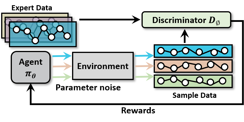
Updating discriminator ($\mathcal{D}_{\phi})$. In GAIL, Equation (4) draws a connection between adversarial network and imitation learning algorithm. The policy $\pi_{\theta}$ is trained to confuse a discriminator $\mathcal{D}_{\phi}$. The $\mathcal{D}_{\phi}$ tries to distinguish between the distribution of trajectories which is sampled by the policy $\pi_{\theta}$ and the expert trajectories $\mathcal{T}_{E}$. The trajectories are consist of state-action pair $(s,a)$. The discriminator takes the role of a reward function in AILSRS shown in Fig. 1; and thus the result of the discriminator is used to train the policy $\pi_{\theta}$. Therefore, the performance of the discriminator is important in our method. However, since the policy $\pi_{\theta}$ is updated every iteration, sampled trajectories which are used to train the discriminator are changed. The training of the discriminator is not stabilized; and thus it makes the inaccurate reward signal. As a result, the policy is perturbated during update step [26, 21]. In AILSRS, the loss function of least square GAN (LS-GAN) is used to train a discriminator $\mathcal{D}_{\phi}$ [27]. The objective function of the discriminator is as follows:

$$\begin{multlined}\mathop{\mathrm{argmin}}\limits_{\phi}L_{LS}(\mathcal{D})=\frac{1}{2}\mathbb{E}_{\pi_{E}}\left[(\mathcal{D}_{\phi}(s,a)-b)^{2}\right]+\\ \frac{1}{2}\mathbb{E}_{\pi_{\theta}}\left[(\mathcal{D}_{\phi}(s,a)-a)^{2}\right]\end{multlined}\mathop{\mathrm{argmin}}\limits_{\phi}L_{LS}(\mathcal{D})=\frac{1}{2}\mathbb{E}_{\pi_{E}}\left[(\mathcal{D}_{\phi}(s,a)-b)^{2}\right]+\\ \frac{1}{2}\mathbb{E}_{\pi_{\theta}}\left[(\mathcal{D}_{\phi}(s,a)-a)^{2}\right]$$ (11)

where $a$ and $b$ are the target discriminator labels for the sampled trajectories from the policy $\pi_{\theta}$ and the expert trajectories. In Equation (4), sampled trajectories which are far from the expert trajectories but on the correct side of the decision boundary are almost not penalized by sigmoid cross-entropy loss. In a contrast, the least-squares loss function (11) penalizes the sampled trajectories which are far from the expert trajectories on either side of decision boundary [27]. Therefore, the stability of training is improved; and it leads the discriminator to give accurate reward signals to the update step. In LS-GAN, $a$ and $b$ have relationship $b-a=2$ for Equation (11) to be Pearson $\mathcal{X}^{2}$ divergence [27]. However, we use $a=0$ and $b=1$ as the target discriminator labels. The result of the discriminator $\mathcal{D}_{\phi}$ in the range of 0 to 1. These values are chosen by empirical results.

Hyperparameters : $\alpha$ step size, $N$ number of sampled directions per iteration, $\delta$ a zero mean Gaussian vector, $\nu$ a positive real number standard deviation of the exploration noise

Initialize : $\theta_{0}=\mathbb{0}\in\mathbb{R}^{p\times n},\mu_{0}=\mathbb{0}\in\mathbb{R}^{n},$ and $\sum_{0}=\mathbb{I}_{n}\in\mathbb{R}^{n\times n}$

1 while $t\leq$ Max Iteration do

2      Sample $\mathbb{\delta_{t}}=\left\{\delta_{1},\delta_{2},...,\delta_{N};\delta_{i}\in\mathbb{R}^{p\times n}\right\}$ with i.i.d.

3      Collect $2N$ rollouts and their corresponding rewards using the $2N$ policies.

4      $\pi_{t,i,+(s)}=(\theta_{t}+\nu\delta_{i})diag(\sum_{t})^{−1/2}(s-\mu_{t})$

5      $\pi_{t,i,-(s)}=(\theta_{t}-\nu\delta_{i})diag(\sum_{t})^{−1/2}(s-\mu_{t})$

6      for $i\in\left\{1,2,\dots,N\right\}$

7      Update discriminator parameter $\phi_{t}$ :

8      $\nabla_{\phi_{t}}L_{LS}=\frac{1}{2}\mathbb{E}_{\pi_{E}}\left[(\nabla_{\phi_{t}}\mathcal{D}_{\phi_{t}}(s,a)-b)^{2}\right]$

9      $+\frac{1}{2}\mathbb{E}_{\pi_{\theta}}\left[(\nabla_{\phi}\mathcal{D}_{\phi_{t}}(s,a)-a)^{2}\right]$

10      Update the policy parameter $\theta_{t}$ :

11      $\theta_{t+1}=\theta_{t}+\frac{\alpha}{N\sigma_{R}}\sum^{N}_{i=1}{\left[r(\pi_{t,(i),+})-r(\pi_{t,(i),-})\right]\delta_{(i)}}$

12      where trajectories $T$ sampled from $\pi_{(t,(i),\pm)}$

13      and $r(\pi_{t,(i),\pm})=\mathbb{E}_{(s,a)\thicksim\pi_{t,(i),\pm}}\left[-\log(1-\mathcal{D}_{\phi_{t}}(T))\right]$

14      Set $\mu_{t+1}$, $\sum_{t+1}$ to be the mean and covariance of the states encountered from the start of training.

15      $t$ = $t+1$

16 end while

Algorithm 2 Adversarial Imitation Learning through Simple Random Search (AILSRS)

Updating policy ($\pi_{\theta}$). The discriminator in AILSRS is interpreted as a reward function for which the policy optimizes. The form of reward signal is as follows:

$$\begin{multlined}r_{\pi_{\theta}}(s,a)=-\log(1-\mathcal{D}_{\phi}(s,a))\end{multlined}r_{\pi_{\theta}}(s,a)=-\log(1-\mathcal{D}_{\phi}(s,a))$$ (12)

This means that if the trajectories sampled from the policy $\pi_{\theta}$ is similar to expert trajectories, the policy $\pi_{\theta}$ gets higher reward $r_{\pi_{\theta}}(s,a)$. The policy $\pi_{\theta}$ is updated to maximize the discounted sum of rewards given by the discriminator rather than the reward from the environment as shown in Fig. 1. The objective of AILSRS can be described:

$$\begin{multlined}\mathop{\mathrm{argmax}}\limits_{\theta}\mathbb{E}_{(s,a)\thicksim\pi_{\theta}}\left[r(s,a)\right]=\mathbb{E}_{(s,a)\thicksim\pi_{\theta}}\left[-\log(1-\mathcal{D}_{\phi}(s,a))\right]\end{multlined}\mathop{\mathrm{argmax}}\limits_{\theta}\mathbb{E}_{(s,a)\thicksim\pi_{\theta}}\left[r(s,a)\right]=\mathbb{E}_{(s,a)\thicksim\pi_{\theta}}\left[-\log(1-\mathcal{D}_{\phi}(s,a))\right]$$ (13)

This Equation (13) is connection of adversarial imitation learning and simple random search.

Algorithm. Foremetioned, AILSRS is based on ARS which is model-free reinforcement algorithm. Therefore, AILSRS uses simple linear policy and parameter space exploration for derivative-free policy optimization. The parameters of policy $\pi_{\theta}$ is denoted $\theta$ and hence $\theta$ is a $p\times n$ matrix. The noises $\delta$ of parameter space for exploration are also $p\times n$ matrix. The noises are sampled from a zero mean and $\nu$ standard deviation Gaussian distribution. AILSRS algorithm is shown in Algorithm 2. For each iteration, the noises $\mathbb{\delta}$ which mean search directions in parameter space of policy are chosen randomly (line [2]). Each of the selected $N$ noises make two policies in the current policy $\pi_{\theta}$. We collect $2N$ rollouts and rewards from $N$ noisy policies $\pi_{t,i,\pm}=\theta_{t}\pm\nu\delta_{i}$ (line [3-6]). The high dimensional complex problems have multiple state components with various ranges; and thus it makes the policies to result in large changes in the actions when the same sized changes is not equally influence state components. Therefore, the state normalization is used in AILSRS (line [4-5,14]); and it allows linear policies $\pi_{t,i,\pm}$ to have equal influence for the changes of state components when there are state components with various ranges. [20, 18, 28]. The discriminator $\mathcal{D}_{\phi}$ gives the reward signal to update step. However, since the trajectories for the training of the discriminator can only be obtained from current policies $\pi_{\theta_{t}}$, a discriminator is trained whenever the policy parameter $\theta_{t}$ is updated. The discriminator $\mathcal{D}_{\phi}$ finds the parameter $\phi$ which minimize the objective function (11) (line [7-9]). By using the reward signals from the discriminator, the policy weight is updated in the direction of $\delta$ or $-\delta$ based on the result of $r(\pi_{t,(i),+})-r(\pi_{t,(i),-})$ (line [10-13]). The state normalization is based on the information of the states encountered during the training procedure; and thus $\mu$ and $\sum$ are updated (line [14]).

IV Experiments

Implementation Setting. In this paper, adversarial imitation learning through simple random search (AILSRS) is implemented with Python/TensorFlow [29]. Multi-GPU platform (equipped with the 2 NVIDIA Titan XP GPUs using 1405 MHz main clock and 12 GB memory) was used for training and evaluation the proposed method. The performance of AILSRS is evaluated on the MuJoCo locomotion tasks [30, 31]. The OpenAI Gym provides benchmark reward functions for Gym environments; and it is used to evaluate the performance of AILSRS. Evaluation on three random seeds is widely adopted in the researches. Therefore, We wanted to show the performance of AILSRS in an equally competitive position [20, 18, 17, 21]. The experiment is implemented with 1, 3 and 5 random seeds of the MuJoCo tasks. The hyperparameters were summarized in Table I. Results show that AILSRS achieves rewards from expert trajectories in various random seed evaluation. Each training curve was smoothed through a Gaussian filter for the average of the experimental results. The discriminator network for AILSRS is consist of two hidden layer of 100 units, with $tanh$ non-linearities in between layers. In the experiment, BC used the same structure policy as AILSRS.

TABLE I: Hyperparameters

Hyperparameters	Descriptions
$\alpha$ update step	0.02
$N$ number of direction	320
$\nu$ standard deviation of noise	0.03
Max iteration of each rollout	1000
Max Training iteration	100000
Discriminator learning rate	0.00025
Discriminator batch size	episode length of each rollout
Discriminator training iteration	3

(a) HalfCheetah-v2

(b) Hopper-v2

(c) Walker-v2

(d) Swimmer-v2

Figure 2: The performance of trained policy according to the set number of expert trajectories

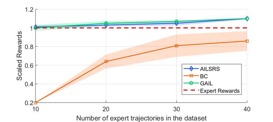
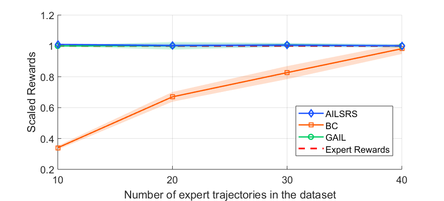
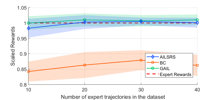
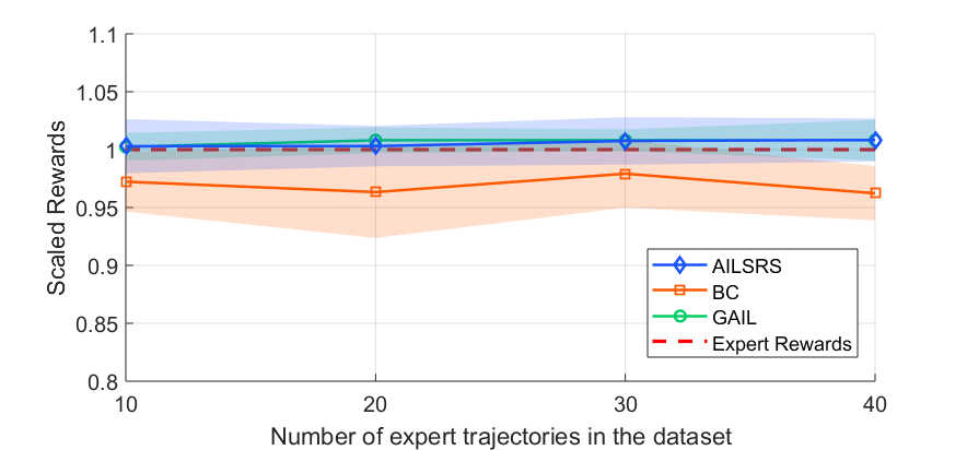
Sample Efficiency Experiments. The purpose of experiments of Fig. 2 was to show the sample efficiency of AILSRS. In Fig. 2, the blue lines means that the performance of the trained policies by AILSRS for the MuJoCo locomotion tasks. To compare the difference between the performance of AILSRS and GAIL, the experiments is executed on the HalfCheetah-v2, Swimmer-v2, Hopper-v2, and Walker-v2. In this experiment, in order to assess performance variability, repeated-measures were used based on three random seeds. Behavior cloning (BC) is used to accelerate the training policies for AILSRS and GAIL on HalfCheetah-v2 experiments. We evaluate AILSRS against two benchmars:

• Behavior Cloning (BC) : The policy is trained with supervised learning, using Adam optimizer. The policy parameter is trained to satisfy Equation (1).

• Generative Adversarial Imitation Learning (GAIL) : The algorithm of [17] using the objective function (4). The implementation is based on OpenAI baseline with deterministic/stochastic policy GAIL [32].

Fig. (2) presents that AILSRS achieve reasonable performance on MuJoCO locomotion tasks. On average, the performance of AILSRS were shown to learn stable policies.

In the HalfCheetah-v2 experiment, we used expert trajectories with an average reward of 4632. At this time, BC has the worst performances of 1000 $\pm$ 10.32 when 10 expert trajectories are the least. However, as the number of expert trajectories increases, performance is better, and finally, performance is better than 4120 $\pm$ 129.12 expert rewards. However, the standard deviation of the performance is very large and shows that it does not reach the expert rewards.

In the case of HalfCheetah-v2, I used imitation learning using GAIL after learning some policy through BC. As a result, GAIL shows the ability to reach expert rewards in the lowest 10 expert trajectories in the experimental environment. And as expert trajectories increase, they perform consistently better than expert rewards. And, unlike BC, the standard deviations of performance are very small, and we can see that stable policy has been learned.

As with GAIL, AILSRS pre-learned the policy through BC and imitation learning was done using AILSRS. In the HalfCheetah-v2 environment, AILSRS also reached 4632, the expert rewards in lesser expert trajectories, and shows less standard deviation performance. In addition, unlike BC, you can see that it performs better by interacting with the environment and learning.

We used expert trajectories with an average reward of 3245 in the Hopper-v2 experiment. At this time, BC has the worst performances of 1200 $\pm$ 10.325 when 10 expert trajectories are the least. As the number of Expert trajectories increases, the performance is similar to the expert rewards of 3224 $\pm$ 15.413, as in HalfCheetah-v2. In the case of Hopper-v2, BC is more stable than HalfCheetah-v2. In the Hopper-v2 experiment, both GAIL and AILSRS did not use BC. GAIL has the lowest number of expert trajectories (10), and it shows stable performance comparable to expert rewards. AILSRS, like GAIL, shows stable performance reaching expert rewards in fewer expert trajectories.

Expert trajectories were used to show expected rewards of 1021 for Walker, and data showing 362 expected rewards for Swimmer. Walker and Swimmer show that all three benchmark algorithms perform well compared to HalfCheetah-v2 and Hopper-v2. In the Walker-v2 experiment, BC showed performance of 862.745 $\pm$ 30.62 for 10 expert rewards, and 890.823 $\pm$ 31.23 for 30 expert trajectories on average. I give. In all experiments, performance is somewhat less than the other algorithms, and the performance of the learned policy is also less stable. In both GAIL and AILSRS, we show that we are effectively learning policy within the performance range of 1021 $\pm$ 51.05 for Expert rewards.

In the Swimmer-v2 experiment, all three benchmark algorithms, such as Walker-v2, show good performance. BC shows performance of 352.95 + - 9.16 in 10 expert trjaectories, and is closer to the performance of the most expert than previous experiments. The rest of the Swimmer-v2 experiment shows similar good performance.

GAIL and AILSRS Like other experiments, it shows performance equivalent to expert rewards. At the same time, it shows a small standard deviation of about 4.51 and shows stable learning performance.

Overall, these results indicate that the random search in the parameter space of policies can be used to imitation learning. Through this section we demonstrate that the performance of the proposed AILSRS shows competitive performance comparing with BC and GAIL. AILSRS showed the successful learning of expert trajectories without direct reward of environment on MuJoCo locomotion tasks. Together these results provide important possibility into the imitation learning using random search with simple linear policies.

(a) HalfCheetah-v2

(b) Hopper-v2

(c) Walker-v2

(d) Swimmer-v2

Figure 3: An evaluation of AILSRS on the OpenAI Gym and mujoco locomotion tasks. The training curves are averaged for each random seed experiments.

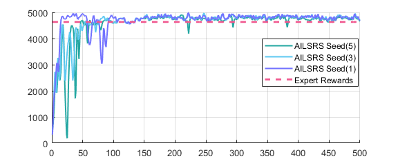
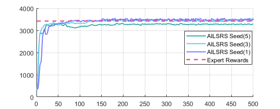
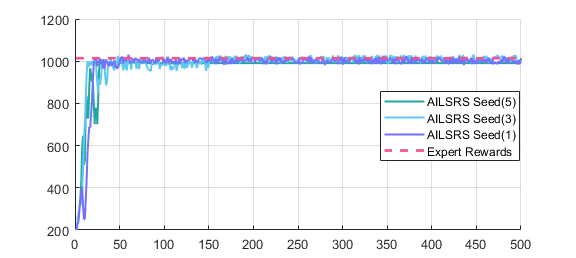
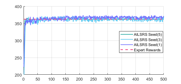
Training Curve. The this sub section of the experiments was concerned with the training stability when we use multiple random seeds. Fig. 3 shows the training curve of Mujoco locomotion tasks in AILSRS. Each experiment shows the results of learning by increasing the number of random seeds. The average of 5 randomly selected experimental out of 20 experimental results is smoothed through a Gaussian filter. Graph made.

In the case of HalfCheetah-v2, it shows that the trained policies in 1, 3 and 5 random seed environments reaches the expert’s reward. However, as the number of random seeds increases, the learning process becomes unstable. In case of hopper-v2, it shows that reaching expert rewards when 1 and 3 random seeds are reached, but it is slightly less than 5 when it is 5. For Walker-v2 and Swimmer-v2, all experimental results show that they reach expert rewards. This graph shows that AILSRS can quickly and successfully learn policies from expert trajectories without a direct reward signal of the environment, even if the number of random seeds increases to one, three, and five. However, in the case of Ant-v2 and Humanoid-v2 which are difficult problems in Mujoco locomotion tasks, the learning speed is very slow, and the environment and analysis of the proposed algorithm are still necessary for the environment.

V Concluding Remarks

The proposed simple random search based imitation learning method is not only a derivative free but aloso model-free reinforcement learning algorithm. Furthermore, the simple linear policies are used to control complex dynamic tasks. It shows competitive performance on MuJoCo locomotion tasks. The simple update step makes the algorithm to be facile; and thus it makes the reconstruction results is able to get reasonable performance easily.

By comparing the performance of the proposed model with complex deep reinforcement learning based imitation learning, we demonstrated that simple random search based imitation learning could be used to train linear policies that achieve reasonable performance on the MuJoCo locomotion tasks.

This results can be a breakthrough to the common belief that random searches in the parameter space of policy can not be competitive in terms of performance. However, the proposed method was not able to get competitive performance on the Ant-v2 and Humanoid-v2 within reasonable training time. Therefore, since the proposed method is simple on-policy algorithm, we can perform extensive research as future research directions.

References

- [1] V. Mnih, K. Kavukcuoglu, D. Silver, A. Graves, I. Antonoglou, D. Wierstra, and M. Riedmiller, “Playing atari with deep reinforcement learning,” arXiv preprint arXiv:1312.5602, 2013.
- [2] S. Levine and V. Koltun, “Guided policy search,” in International Conference on Machine Learning, 2013, pp. 1–9.
- [3] J. Schulman, S. Levine, P. Abbeel, M. Jordan, and P. Moritz, “Trust region policy optimization,” in International Conference on Machine Learning, 2015, pp. 1889–1897.
- [4] T. P. Lillicrap, J. J. Hunt, A. Pritzel, N. Heess, T. Erez, Y. Tassa, D. Silver, and D. Wierstra, “Continuous control with deep reinforcement learning,” arXiv preprint arXiv:1509.02971, 2015.
- [5] D. Horgan, J. Quan, D. Budden, G. Barth-Maron, M. Hessel, H. Van Hasselt, and D. Silver, “Distributed prioritized experience replay,” arXiv preprint arXiv:1803.00933, 2018.
- [6] L. Busoniu, R. Babuska, and B. De Schutter, “A comprehensive survey of multiagent reinforcement learning,” IEEE Transactions on Systems, Man, And Cybernetics-Part C: Applications and Reviews, 38 (2), 2008, 2008.
- [7] S. Lange, M. Riedmiller, and A. Voigtlander, “Autonomous reinforcement learning on raw visual input data in a real world application,” in Neural Networks (IJCNN), The 2012 International Joint Conference on. IEEE, 2012, pp. 1–8.
- [8] J. Kober and J. Peters, “Reinforcement learning in robotics: A survey,” in Reinforcement Learning. Springer, 2012, pp. 579–610.
- [9] H. Zhu, A. Gupta, A. Rajeswaran, S. Levine, and V. Kumar, “Dexterous manipulation with deep reinforcement learning: Efficient, general, and low-cost,” arXiv preprint arXiv:1810.06045, 2018.
- [10] C. Chen, A. Seff, A. Kornhauser, and J. Xiao, “Deepdriving: Learning affordance for direct perception in autonomous driving,” in 2015 IEEE International Conference on Computer Vision (ICCV). IEEE, 2015, pp. 2722–2730.
- [11] J. Schulman, F. Wolski, P. Dhariwal, A. Radford, and O. Klimov, “Proximal policy optimization algorithms,” arXiv preprint arXiv:1707.06347, 2017.
- [12] P. Henderson, R. Islam, P. Bachman, J. Pineau, D. Precup, and D. Meger, “Deep reinforcement learning that matters,” arXiv preprint arXiv:1709.06560, 2017.
- [13] R. Islam, P. Henderson, M. Gomrokchi, and D. Precup, “Reproducibility of benchmarked deep reinforcement learning tasks for continuous control,” arXiv preprint arXiv:1708.04133, 2017.
- [14] A. Billard, S. Calinon, R. Dillmann, and S. Schaal, “Robot programming by demonstration,” in Springer handbook of robotics. Springer, 2008, pp. 1371–1394.
- [15] D. Pomerleau, “Rapidly adapting artificial neural networks for autonomous navigation,” in Advances in neural information processing systems, 1991, pp. 429–435.
- [16] D. A. Pomerleau, “Alvinn: An autonomous land vehicle in a neural network,” in Advances in neural information processing systems, 1989, pp. 305–313.
- [17] J. Ho and S. Ermon, “Generative adversarial imitation learning,” in Advances in Neural Information Processing Systems, 2016, pp. 4565–4573.
- [18] T. Salimans, J. Ho, X. Chen, S. Sidor, and I. Sutskever, “Evolution strategies as a scalable alternative to reinforcement learning,” arXiv preprint arXiv:1703.03864, 2017.
- [19] A. Rajeswaran, K. Lowrey, E. V. Todorov, and S. M. Kakade, “Towards generalization and simplicity in continuous control,” in Advances in Neural Information Processing Systems, 2017, pp. 6550–6561.
- [20] H. Mania, A. Guy, and B. Recht, “Simple random search provides a competitive approach to reinforcement learning,” arXiv preprint arXiv:1803.07055, 2018.
- [21] Anonymous, “Generative adversarial self-imitation learning,” in Submitted to International Conference on Learning Representations, 2019, under review.
- [22] P. Henderson, W.-D. Chang, P.-L. Bacon, D. Meger, J. Pineau, and D. Precup, “Optiongan: Learning joint reward-policy options using generative adversarial inverse reinforcement learning,” arXiv preprint arXiv:1709.06683, 2017.
- [23] J. Matyas, “Random optimization,” Automation and Remote control, vol. 26, no. 2, pp. 246–253, 1965.
- [24] Y. Nesterov and V. Spokoiny, “Random gradient-free minimization of convex functions,” Université catholique de Louvain, Center for Operations Research and Econometrics (CORE), Tech. Rep., 2011.
- [25] A. D. Flaxman, A. T. Kalai, and H. B. McMahan, “Online convex optimization in the bandit setting: gradient descent without a gradient,” in Proceedings of the sixteenth annual ACM-SIAM symposium on Discrete algorithms. Society for Industrial and Applied Mathematics, 2005, pp. 385–394.
- [26] J. Sorg, R. L. Lewis, and S. P. Singh, “Reward design via online gradient ascent,” in Advances in Neural Information Processing Systems, 2010, pp. 2190–2198.
- [27] X. Mao, Q. Li, H. Xie, R. Y. Lau, Z. Wang, and S. P. Smolley, “Least squares generative adversarial networks,” in Computer Vision (ICCV), 2017 IEEE International Conference on. IEEE, 2017, pp. 2813–2821.
- [28] A. Nagabandi, G. Kahn, R. S. Fearing, and S. Levine, “Neural network dynamics for model-based deep reinforcement learning with model-free fine-tuning,” in 2018 IEEE International Conference on Robotics and Automation (ICRA). IEEE, 2018, pp. 7559–7566.
- [29] M. Abadi, A. Agarwal, P. Barham, E. Brevdo, Z. Chen, C. Citro, G. S. Corrado, A. Davis, J. Dean, M. Devin, S. Ghemawat, I. Goodfellow, A. Harp, G. Irving, M. Isard, Y. Jia, R. Jozefowicz, L. Kaiser, M. Kudlur, J. Levenberg, D. Mané, R. Monga, S. Moore, D. Murray, C. Olah, M. Schuster, J. Shlens, B. Steiner, I. Sutskever, K. Talwar, P. Tucker, V. Vanhoucke, V. Vasudevan, F. Viégas, O. Vinyals, P. Warden, M. Wattenberg, M. Wicke, Y. Yu, and X. Zheng, “TensorFlow: Large-scale machine learning on heterogeneous systems,” 2015, software available from tensorflow.org. [Online]. Available: http://tensorflow.org/
- [30] E. Todorov, T. Erez, and Y. Tassa, “Mujoco: A physics engine for model-based control,” in Intelligent Robots and Systems (IROS), 2012 IEEE/RSJ International Conference on. IEEE, 2012, pp. 5026–5033.
- [31] G. Brockman, V. Cheung, L. Pettersson, J. Schneider, J. Schulman, J. Tang, and W. Zaremba, “Openai gym,” 2016.
- [32] P. Dhariwal, C. Hesse, O. Klimov, A. Nichol, M. Plappert, A. Radford, J. Schulman, S. Sidor, Y. Wu, and P. Zhokhov, “Openai baselines,” https://github.com/openai/baselines, 2017.