Correcting a Nonparametric Two-sample Graph Hypothesis Test for Graphs with Different Numbers of Vertices with Applications to Connectomics

Abstract

Random graphs are statistical models that have many applications, ranging from neuroscience to social network analysis. Of particular interest in some applications is the problem of testing two random graphs for equality of generating distributions. Tang et al. (2017) propose a test for this setting. This test consists of embedding the graph into a low-dimensional space via the adjacency spectral embedding (ASE) and subsequently using a kernel two-sample test based on the maximum mean discrepancy. However, if the two graphs being compared have an unequal number of vertices, the test of Tang et al. (2017) may not be valid. We demonstrate the intuition behind this invalidity and propose a correction that makes any subsequent kernel- or distance-based test valid. Our method relies on sampling based on the asymptotic distribution for the ASE. We call these altered embeddings the corrected adjacency spectral embeddings (CASE). We also show that CASE remedies the exchangeability problem of the original test and demonstrate the validity and consistency of the test that uses CASE via a simulation study. Lastly, we apply our proposed test to the problem of determining equivalence of generating distributions in human connectomes extracted from diffusion magnetic resonance imaging (dMRI) at different scales.

Keywords: Adjacency Spectral Embedding, Latent Position Graph, Random Dot Product Graph

1 Introduction

Modeling data as random graphs is ubiquitous in many application domains of statistics. For example, in neuroscience, it is common to view a connectome as a graph with vertices representing neurons, and edges representing synapses (Priebe et al., 2017). In document analysis, the corpus of text can be viewed as a graph with vertices taken to be documents or authors, and edges as the citations (de Solla Price, 1965). In social network analysis, a network can be modeled as a graph with vertices being individual actors or organizations, and edges being representing the degree of communication between them (Wasserman and Faust, 1994).

The first random graph model was proposed in 1959 by E. N. Gilbert. In his short paper, he considered a graph in which the probability of an edge between any two vertices was a Bernoulli random variable with common probability $p$ (Gilbert, 1959). Almost concurrently, Erdös and Rényi developed a similar random graph model with a constrained number of edges that are randomly allocated in a graph. They also provided a detailed analysis of the probabilities of the emergence of certain types of subgraphs within graphs developed both by them and Gilbert (Erdös and Rényi, 1960). Nowadays, the graphs in which edges arise independently and with common probability $p$ are known as Erdös-Rényi (ER) graphs.

Latent position random graph models consitute a diverse class of random graph models that are much more flexible than the ER model. A vertex in a latent position graph is associated with an element in a latent space $\mathcal{X}$, and the probability of an edge between any two vertices is given by a link function $g:\mathcal{X}\times\mathcal{X}\to[0,1]$ (Hoff et al., 2002). The model draws inspiration from social network analysis, in which the members are thought of as vertices, and the latent positions are differing “interests”. Latent position random graphs are a submodel of the independent edge graphs, that is, graphs in which the edge probabilities are indpendent, conditioned on a matrix of probabilities. The theory of latent positions graphs is also closely related to that of graphons (Lovász, 2012); for discussion on this relationship, see, for example, Lei (2018) or Rubin-Delanchy (2020).

One example of latent position graphs relevant to this discussion is the random dot product graph (RDPG). An RDPG is a latent position graph in which the latent space is an appropriately constrained Euclidian space $\mathbb{R}^{d}$, and the link function is the inner product of the $d$-dimensional latent positions (Athreya et al., 2018). Despite their relative simplicity, suitably high-dimensional RDPGs can provide useful approximations of general latent position and independent edge graphs, as long as their matrix of probabilities is positive semidefinite (Tang et al., 2013).

The well-known stochastic blockmodel (SBM), in which each vertex belongs to one of $K$ blocks, with connection probabilities determined solely by block membership (Holland et al., 1983), can be represented as an RDPG for which all vertices in a given block have the same latent positions. Furthermore, common extensions of SBMs, namely degree-corrected SBMs (Karrer and Newman, 2011), mixed membership SBMs (Airoldi et al., 2008), and degree-corrected mixed membership SBMs (Jin et al., 2017) can also be framed as RDPG. There is, however, a caveat, similar to the one for approximating independent edge graphs with RDPG: only SBM graphs with positive semidefinite block probability matrix can be formulated in the context of RDPG. Rubin-Delanchy et al. (2022) present a generalization of RDPGs, called the generalized random dot product graph (GRDPG) that allows to drop the positive semidefiniteness requirements in both cases. Although the generalization of many estimation and inference procedures from RDPGs to GRDPGs is straightforward, their theory, particularly of latent distribution testing, is not yet as developed as that of RDPG. Thus, we limit the scope of this work to RDPG.

The problem of whether the two graphs are “similar” in some appropriate sense arises naturally in many fields. For example, two different brain graphs may be tested for the similarity of the connectivity structure (Chung et al., 2022), or user behavior may be compared between different social media platforms. Testing for similarity also has applications in more intricate network analysis techniques, such as hierarchical community detection (Lyzinski et al., 2017; Li et al., 2020). Despite the multitude of applications, network comparison is a relatively nascent field, and comparatively few techniques currently exist (Lyzinski et al., 2017). There have been several tests assuming the random graphs have the same set of nodes, such as Tang et al. (2017); Levin et al. (2017); Ghoshdastidar et al. (2017); Li and Li (2018); Levin and Levina (2019), and Arroyo et al. (2021). Other approaches designed for fixed models and related problems, include Rukhin and Priebe (2011); Asta and Shalizi (2015); Lei (2016); Bickel and Sarkar (2016); Maugis et al. (2020); Chen and Lei (2018); Gangrade et al. (2019) and Fan et al. (2022), to name a few. In Ghoshdastidar et al. (2020), the authors formulate the two-sample testing problem for graphs of different orders more generally.

Of particular interest is Tang et al. (2017), in which the authors propose a nonparametric test for the equality of the generating distributions for a pair of random dot product graphs. This test does not require the graphs to have the same set of nodes or be of the same order. It relies on embedding the adjacency matrices of the graphs into Euclidean space, followed by a kernel two-sample test of Gretton et al. (2012) performed on these embeddings. The exact finite-sample distribution of the test statistics is unknown, but it can be estimated using a permutation test, or approximated using the $\chi^{2}$-distribution. Unfortunately, despite the theorem stating that in the limit, even for graphs of differing orders, the statistic using the two embeddings converges to the statistic obtained using the true but unknown latent positions, the test is not always valid for finite graphs of differing orders.

The invalidity arises from the fact that the approximate finite-sample variance of the adjacency spectral embedding depends on the number of vertices (Athreya et al., 2016). Hence, the distributions of the estimates of the latent positions for the two graphs might not be the same, even if the true distributions of the latent positions are equivalent. The test of Gretton et al. (2012) is sensitive to the differences induced by this incongruity and as a result may reject more often than the intended significance level. In this work, we present a method for modifying the embeddings before computing of the test statistic. Using this correction makes the test for the equivalence of latent distributions valid even when the two graphs have an unequal number of vertices.

The remainder of the paper is structured as follows. In Section 2, we review the random dot product graph, and discuss its relationship with Erdös-Rényi, stochastic blockmodel and other random graph models. We also discuss results associated with the adjacency spectral embedding of an RDPG, such as consistency for the true latent positions and asymptotic normality, and we review the original nonparametric two-sample hypothesis test for the equality of the latent distributions. There we also briefly discuss generalizing the ASE procedure to weighted and/or directed graphs. Then, in Section 3, we give an intuition as to why this test increases in size as the orders of the two graphs diverge from each other. We also present our approach to correcting the adjacency spectral embeddings in a way that makes them exchangeable under the null hypothesis of the test for the equivalence of the latent distribution. We demonstrate the validity and consistency of the test that uses the corrected adjacency spectral embeddings across a variety of settings in Section 4. In Section 5, we demonstrate that failing to correct for the difference in distributions can lead to significant inferential consequences in real world applications, such as the setting of brain graphs obtained from diffusion magnetic resonance imaging (dMRI). Furthermore, we show that the test is able to meaningfully differentiate between scans within the same subject and different subjects. We conclude and discuss our findings in Section 6.

1.1 Notation

We use the terminology “order” for the number of vertices in a graph. We denote scalars by lowercase letters, vectors by bold lowercase letters and matrices by bold capital letters. For example, $c$ is a scalar, $\boldsymbol{x}$ is a vector, and $\boldsymbol{H}$ is a matrix. For any matrix $\boldsymbol{H}$, we let $\boldsymbol{H}_{ij}$ denote its $i,j$th entry. For ease of notation, we also denote $\boldsymbol{H}_{i}$ to be the column vector obtained by transposing the $i$-th row of $\boldsymbol{H}$. Formally, $\boldsymbol{H}_{i}=\left(\boldsymbol{H}_{i\cdot}\right)^{T}$. In the case where we need to consider a sequence of matrices, we will denote such a sequence by $\boldsymbol{H}^{(n)}$, where $n$ is the index of the sequence. Whether a particular scalar, vector or a matrix is a constant or a random variable will be stated explicitly or be apparent from context. Unbold capital letters denote sets or probability distributions. For example, $F$ is a probability distribution. The exception to this rule is $K$ which is always used to denote the number of blocks in a stochastic blockmodel.

2 Preliminaries

2.1 Models

We begin by defining random dot product graphs.

Definition 1 ($d$-dimensional random dot product graph (RDPG)).

Let $F$ be a distribution on a set $\mathcal{X}\subset\mathbb{R}^{d}$ such that $\langle\boldsymbol{x},\boldsymbol{x}^{\prime}\rangle\in[0,1]$ for all $\boldsymbol{x},\boldsymbol{x}^{\prime}\in\mathcal{X}$. We say that $(\boldsymbol{X},\boldsymbol{A})\sim RDPG(F,n)$ is an instance of a random dot product graph (RDPG) if $\boldsymbol{X}=[\boldsymbol{X}_{1},\ldots,\boldsymbol{X}_{n}]^{T}$ with $\boldsymbol{X}_{1}.\ldots,\boldsymbol{X}_{n}\stackrel{{\scriptstyle iid}}{{\sim}}F$ and $\boldsymbol{A}\in\left\{0,1\right\}^{n\times n}$ is a symmetric hollow matrix whose entries in the upper triangle are conditionally independent given $\boldsymbol{X}$ and satisfy

$$\boldsymbol{A}_{ij}|\boldsymbol{X}\sim Bernoulli(\boldsymbol{X}_{i}^{T}\boldsymbol{X}_{j}) i<j.$$

We refer to $\boldsymbol{X}_{1}.\ldots,\boldsymbol{X}_{n}$ as the latent positions of the corresponding vertices.

Remark 1.

It is easy to see that if $(\boldsymbol{X},\boldsymbol{A})\sim RDPG(F,n)$, then $E[\boldsymbol{A}|\boldsymbol{X}]=\boldsymbol{X}\boldsymbol{X}^{T}$.

Remark 2.

Nonidentifiability is an intrinsic property of random dot product graphs. For any matrix $\boldsymbol{X}$ and any orthogonal matrix $\boldsymbol{W}$, the inner product between any rows $i,j$ of $\boldsymbol{X}$ is identical to that between the rows $i,j$ of $\boldsymbol{X}\boldsymbol{W}$. Hence, for any probability distribution $F$ on $\mathcal{X}$ and orthogonal operator $\boldsymbol{W}$, the adjacency matrices $\boldsymbol{A}$ and $\boldsymbol{B}$, generated according to $(\boldsymbol{X},\boldsymbol{A})\sim RDPG(F,n)$ and $(\boldsymbol{Y},\boldsymbol{B})\sim RDPG(F\circ\boldsymbol{W},n)$, respectively, are identically distributed. Here, the notation $F\circ\boldsymbol{W}$ means that if $\boldsymbol{X}\sim F$, then $\boldsymbol{X}\boldsymbol{W}\sim F\circ\boldsymbol{W}$.

Constraining all latent positions to a single value leads to an Erdös-Rényi (ER) random graph.

Definition 2 (Erdös-Rényi graphs (ER)).

We say that a graph $(\boldsymbol{X},\boldsymbol{A})\sim RDPG(F,n)$ is an Erdös-Rényi (ER) graph with an edge probability $p^{2}$ if $F$ is a pointmass at $p$. In this case, we write $\boldsymbol{A}\sim ER(n,p^{2})$.

Another random graph model that can be framed in the context of random dot product graphs is the stochastic blockmodel (SBM) (Holland et al., 1983). In the SBM, the vertex set is thought of as being partitioned into $K$ groups, called blocks, and the probability of an edge between two vertices is determined by their block memberships. The partitioning, or assignment, of the vertices is usually itself random and mutually independent. Formally, we can define SBMs in terms of the RDPG model as follows.

Definition 3 ((Positive semidefinite) stochastic blockmodel (SBM)).

Denote $\delta_{\boldsymbol{z}}$ as the Dirac delta measure at $\boldsymbol{z}$. We say that a graph $(\boldsymbol{X},\boldsymbol{A})\sim RDPG(F,n)$ is a (positive semidefinite) stochastic blockmodel (SBM) with $K$ blocks if the distribution $F$ is a mixture of $K$ point masses,

$$F=\sum_{i=1}^{K}\pi_{i}\delta_{\boldsymbol{Z}_{i}},$$ (1)

where $\boldsymbol{\pi}=\left[\pi_{1},\ldots,\pi_{K}\right]\in(0,1)^{K}$ satisfying $\sum_{i=1}^{K}\pi_{i}=1$, and the distinct latent positions are given by $\boldsymbol{Z}=\left[\boldsymbol{Z}_{1},\ldots,\boldsymbol{Z}_{K}\right]^{T}\in\mathbb{R}^{K\times d}$, with $\boldsymbol{Z}_{i}^{T}\boldsymbol{Z}_{j}\in[0,1]$ $\forall i,j$. In this case we also write $\boldsymbol{A}\sim SBM\left(n,\boldsymbol{\pi},\boldsymbol{P}\right)$, where $\boldsymbol{P}:=\boldsymbol{Z}\boldsymbol{Z}^{T}\in\mathbb{R}^{K\times K}$. The matrix $\boldsymbol{P}$ is often referred to as block probability matrix.

Remark 3.

We note that almost everywhere below we use the terms SBM and positive semidefinite SBM interchangeably, as only positive semidefinite block probability matrices can be represented as a product of a matrix of latent positions with transpose of itself, and thus only they can be defined in terms of the RDPG model. We emphasize, however, that the work of Rubin-Delanchy et al. (2022) on the generalized random dot product (GRDPG) extends the construction of RDPG via the indefinite inner product to encompass indefinite SBM and the generalizations thereof.

There are two common generalizations of the stochastic blockmodel: degree-corrected stochastic blockmodel (Karrer and Newman, 2011) and mixed-membership stochastic blockmodel (Airoldi et al., 2008). We present these two models below. The presentations are different from the ones many readers may be familiar with because we present them under the RDPG framework. These definitions coincide with the ones in literature, as covered in Lyzinski et al. (2014); Rubin-Delanchy et al. (2017, 2022).

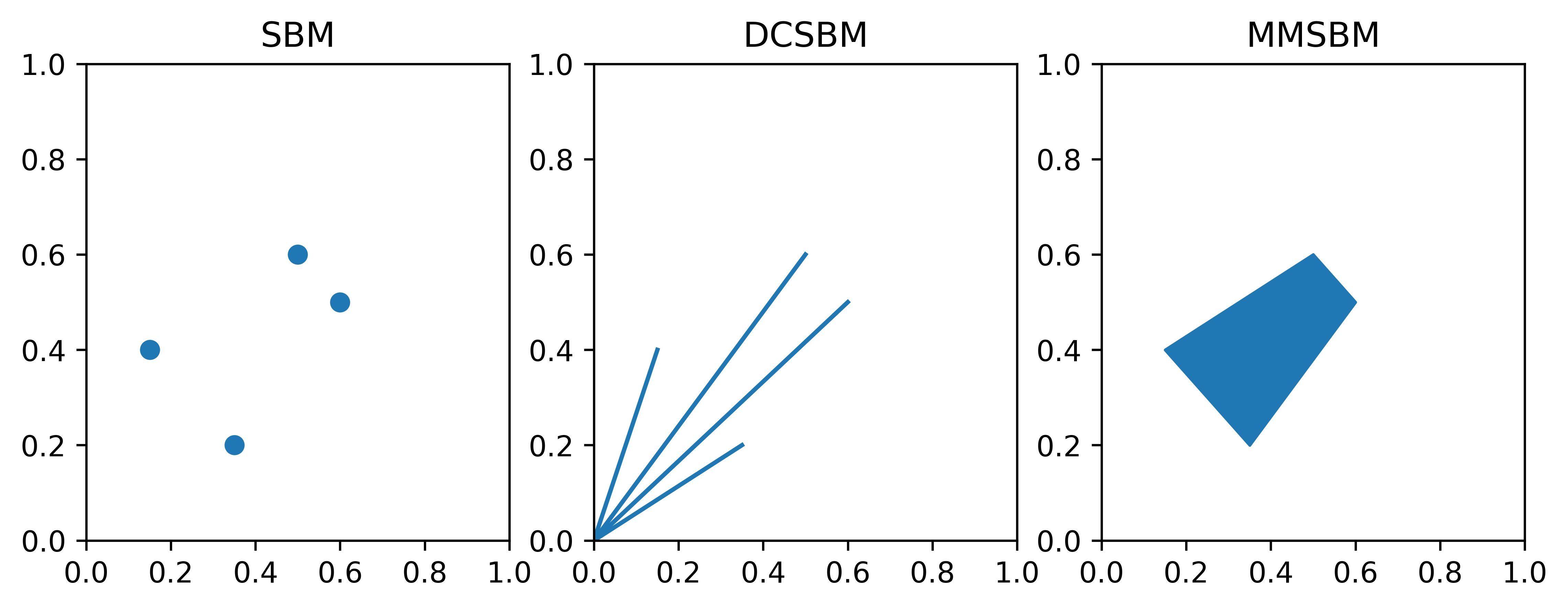
Figure 1: Visualization of the valid latent positions of an arbitrary 2-dimensional SBM with $K=4$ (left), valid latent positions of a DCSBM with the same $\boldsymbol{Z}$ (center) and valid latent positions of an MMSBM with the same $\boldsymbol{Z}$ (right). All three are examples of RDPGs.

The degree-corrected stochastic blockmodel allows for vertices within each block to have different expected degrees, which makes it more flexible than the standard SBM and a popular choice to model network data (Karrer and Newman, 2011; Lyzinski et al., 2014).

Definition 4.

(Degree-corrected SBM) We say that a graph $(\boldsymbol{X},\boldsymbol{A})\sim RDPG(F,n)$ is a degree-corrected SBM (DCSBM) with $K$ blocks, if there exists a distribution $F_{m}$, which is a mixture of $K$ point-masses $\boldsymbol{Z}_{1},\ldots,\boldsymbol{Z}_{K}$, as in Definition 3, and a distribution $F_{c}$ on $[0,1]$, such that for all $\boldsymbol{X}_{i}$, there exists $\boldsymbol{Y}_{i}\sim F_{m}$ and $c_{i}\sim F_{c}$, such that $\boldsymbol{X}_{i}=c_{i}\boldsymbol{Y}_{i}$.

That is, any latent position of a vertex in a DCSBM graph can be decomposed into a point $\boldsymbol{Y}_{i}$, chosen among one of the $K$ shared points $\boldsymbol{Z}_{1},\ldots,\boldsymbol{Z}_{K}$, and a scalar $c_{i}$. Note that there is no requirement on $\boldsymbol{Y}_{i}$ and $c_{i}$ to be independent from each other. In other words, the distributions on degree corrections can depend on the block assignments. In essence, the DCSBM generalizes the SBM from an RDPG with a distribution of latent positions over a finite number of points to an RDPG with a distribution of latent positions over a finite number of rays from the origin. Of course, not every point on these rays needs to be in the support of this distribution. Restraining $F_{c}$ to a point-mass at unity recovers the regular SBM. See left and central panels of Figure 1 for a visualization comparing the latent distributions of SBM and DCSBM.

On the other hand, the mixed membership SBM offers more flexibility in block memberships by allowing each vertex to be in a mixture of blocks (Airoldi et al., 2008).

Definition 5.

(Mixed-membership SBM) Denote $\Delta^{d\times 1}$ to be the space of the $(d+1)$-dimensional column vectors starting at the origin and terminating in the $d$-dimensional unit simplex. We say that a graph $(\boldsymbol{X},\boldsymbol{A})\sim RDPG(F,n)$ is a mixed-membership SBM (MMSBM) with $K$ blocks, if there exists a matrix $\boldsymbol{Z}=\left[\boldsymbol{Z}_{1},\ldots,\boldsymbol{Z}_{K}\right]^{T}\in\mathbb{R}^{K\times d}$ and a distribution over $\Delta^{(K-1)\times 1}$, denoted as $F_{m}$, such that for each $\boldsymbol{X_{i}}$, there exists $\boldsymbol{v}_{i}\sim F_{m}$ and $\boldsymbol{X_{i}}=\boldsymbol{Z}^{T}\boldsymbol{v}_{i}$.

That is, any latent position of a vertex in an MMSBM is a convex combination of $K$ shared points, $\boldsymbol{Z}_{1},\ldots,\boldsymbol{Z}_{K}$. The MMSBM generalizes the SBM from an RDPG with latent positions coming from a finite-dimensional mixture of point-masses to an RDPG with latent positions having a distribution over a convex hull formed by a finite number of points. See left and right panels of Figure 1 for a visualization of thereof. Once again, the whole convex hull needs not be in the support of this distribution. If one constrains $F_{m}$ to only have support on a finite set of vectors with 1 in a single entry and 0 in all other, $F_{m}$ collapses to a distribution of point-masses and the model agrees exactly with SBM.

Remark 4.

For graphs with one-dimensional latent positions, any RDPG model is both a DCSBM with a single block and an MMSBM with two blocks. To see this, note that the latent positions all take values in $[0,1]$ (or equivalently $[-1,0]$). This region can be thought of as either a single line segment starting from the origin or as a one-dimensional convex hull between $0$ and $1$.

Remark 5.

Jin et al. (2017) introduced a model that has both the degree heterogeneity of the DCSBM and the flexible memberships of MMSBM. This model can also be formulated in terms of the RDPG. See, for example, Definition 6 of Agterberg et al. (2020).

We reiterate that the SBM with $K$ blocks is a submodel of both the $K$-block DCSBM and the $K$-block MMSBM. Furthermore, both the $K$-block DCSBM and the $K$-block MMSBM are submodels of an RDPG with latent positions in at most $K$ dimensions. Hence, any test for the equality of the latent distributions that is consistent in the RDPG setting will be able to meaningfully distinguish between two graphs generated from two different model subspaces, or between graphs from the same model subspace but with different parameters; for example, between a MMSBM and an SBM, or between two SBMs with different block-probability matrices.

2.2 Adjacency spectral embedding

Inference on random dot product graphs relies on having good estimates of the latent positions of the vertices. One way to estimate the latent positions is to use the adjacency spectral embedding of the graph, defined as follows.

Definition 6 (Adjacency spectral embedding (ASE)).

Let $\boldsymbol{A}$ have eigendecomposition

$$\boldsymbol{A}=\boldsymbol{U}\boldsymbol{\Lambda}\boldsymbol{U}^{\top}+\boldsymbol{U}_{\perp}\boldsymbol{\Lambda}_{\perp}\boldsymbol{U}_{\perp}^{T}$$

where $\boldsymbol{U}$ and $\boldsymbol{\Lambda}$ consist of the top $d$ eigenvectors and eigenvalues (arranged by decreasing magnitude) respectively, and $\boldsymbol{U}_{\perp}$ and $\boldsymbol{\Lambda}_{\perp}$ consist of the bottom $n-d$ eigenvectors and eigenvalues respectively. The adjacency spectral embedding of $\boldsymbol{A}$ into $\mathbb{R}^{d}$ is the $n\times d$ matrix

$$\hat{\boldsymbol{X}}:=\boldsymbol{U}|\boldsymbol{\Lambda}|^{1/2},$$

where the operator $|\cdot|$ takes the entrywise absolute value.

It has been proven in Sussman et al. (2012, 2014) and Lyzinski et al. (2014) that the adjacency spectral embedding provides a consistent estimate of the true latent positions in random dot product graphs. The key to this result is tight concentrations, in both Frobenius and $2\to\infty$ norms, of the ASE about the true latent positions.

Athreya et al. (2016) show that for a $d$-dimensional RDPG with i.i.d. latent positions, the ASE is not only consistent, but also asymptotically normal, in the sense that there exists a sequence of $d\times d$ real orthogonal matrices $\boldsymbol{W}^{(n)}$ such that for any row index $i$, $\sqrt{n}\left(\boldsymbol{W}^{(n)}\hat{\boldsymbol{X}}_{i}^{(n)}-\boldsymbol{X}_{i}^{(n)}\right)$ converges to a (possibly infinite) mixture of multivariate normals.

Theorem 2.1 (RDPG Central Limit Theorem).

Let $(\boldsymbol{X}^{(n)},\boldsymbol{A}^{(n)})\sim RDPG(F,n)$ be a sequence of latent positions and associated adjacency matrices of a $d$-dimensional RDPG according to a distribtuion $F$ in an appropriately constrained region of $\mathbb{R}^{d}$. Also let $\hat{\boldsymbol{X}}^{(n)}$ be the adjacency spectral embedding of $\boldsymbol{A}^{(n)}$ into $\mathbb{R}^{d}$. Let $\Phi(\boldsymbol{z},\boldsymbol{\Sigma})$ denote the cumulative distribution function for the multivariate normal, with mean zero and covariance matrix $\boldsymbol{\Sigma}$, evaluated at $\boldsymbol{z}$. Then there exists a sequence of orthogonal $d\times d$ matrices $\left(\boldsymbol{W}^{(n)}\right)_{n=1}^{\infty}$ such that for each component $i$ and any $\boldsymbol{z}\in\mathbb{R}^{d}$,

$$\lim_{n\to\infty}\mathbb{P}\left[n^{1/2}\left(\hat{\boldsymbol{X}}^{(n)}\boldsymbol{W}^{(n)}-\boldsymbol{X}^{(n)}\right)_{i}\leq\boldsymbol{z}\right]=\int_{\mathrm{supp}F}\Phi\left(\boldsymbol{z},\boldsymbol{\Sigma}(\boldsymbol{x})\right)dF(\boldsymbol{x}),$$

where

$$\boldsymbol{\Sigma}(\boldsymbol{x}) =\Delta^{-1}\mathbb{E}\left[(\boldsymbol{x}^{T}\boldsymbol{X}_{1}-(\boldsymbol{x}^{T}\boldsymbol{X}_{1})^{2})\boldsymbol{X}_{1}\boldsymbol{X}_{1}^{T}\right]\Delta^{-1}$$

and $\Delta=\mathbb{E}\left[\boldsymbol{X}_{1}\boldsymbol{X}_{1}^{T}\right]$ is the second moment matrix.

An intuitive way to restate this result is by identifying that each row $\hat{\boldsymbol{X}}_{i}$ of the ASEs $\hat{\boldsymbol{X}}$ is approximately normal around the true but unknown realization of the latent position of the vertex:

$$\hat{\boldsymbol{X}}_{i}|\boldsymbol{X}_{i}\overset{approx}{\sim}\mathcal{N}\left(\boldsymbol{X}_{i}\boldsymbol{W},\frac{\boldsymbol{\Sigma}(\boldsymbol{X}_{i})}{n}\right)$$

where $\boldsymbol{W}$ is an orthogonal matrix present due to the inherent orthogonal nonidentifiability of the RDPG.

In our work, we will need to estimate the covariance matrix $\boldsymbol{\Sigma}(\boldsymbol{X}_{i})$. The plug-in principle (Bickel and Doksum, 2006) states that one acceptable method of estimating $\boldsymbol{\Sigma}(\boldsymbol{X}_{i})$ is to use the analogous empirical moments:

$$\hat{\boldsymbol{\Sigma}}(\hat{\boldsymbol{X}}_{i}) =\hat{\Delta}^{-1}\left(\frac{1}{n}\sum_{j=1}^{n}\left((\hat{\boldsymbol{X}}_{i}^{T}\hat{\boldsymbol{X}}_{j}-(\hat{\boldsymbol{X}}_{i}^{T}\hat{\boldsymbol{X}}_{j})^{2})\hat{\boldsymbol{X}}_{j}\hat{\boldsymbol{X}}_{j}^{T}\right)\right)\hat{\Delta}^{-1},$$ (2)

where

$$\hat{\Delta} =\frac{1}{n}\sum_{j=1}^{n}\hat{\boldsymbol{X}}_{j}\hat{\boldsymbol{X}}_{j}^{T}.$$

When we are presented with two or more RDPGs that have the same distribution for their latent positions, either by assumption or by prior knowledge, we can leverage this fact and calculate the moments over all graphs at the same time. Conceptually this is similar to using pooled variance in classical one-dimensional two-sample inference.

A corollary of the previous result arises when $(\boldsymbol{X},\boldsymbol{A})\sim RDPG(F,n)$ is a $K$-block stochastic blockmodel. Then, we can condition on the event that $\boldsymbol{X}_{i}$ is assigned to a block $k\in\{1,2,\ldots,K\}$ to show that the conditional distribution of $\hat{\boldsymbol{X}}^{(n)}\boldsymbol{W}^{(n)}-\boldsymbol{X}^{(n)}$ converges to a multivariate normal.

Corollary 2.2.

Assume the setting and notation of Theorem 2.1. Further, assume that $(\boldsymbol{X},\boldsymbol{A})\sim RDPG(F,n)$ is a positive definite stochastic blockmodel, that is, $F$ is a mixture of $K$ point masses $\boldsymbol{Z}_{1},\ldots,\boldsymbol{Z}_{K}$, as per Definition 3. Then there exists a sequence of orthogonal matrices $\boldsymbol{W}_{n}$ such that for all $\boldsymbol{z}\in\mathbb{R}^{d}$ and for any fixed index $i$,

$$\lim_{n\to\infty}\mathbb{P}\left[n^{1/2}\left(\hat{\boldsymbol{X}}^{(n)}\boldsymbol{W}^{(n)}-\boldsymbol{X}^{(n)}\right)_{i}\leq\boldsymbol{z}|\boldsymbol{X}_{i}=\boldsymbol{Z}_{k}\right]=\Phi\left(\boldsymbol{z},\boldsymbol{\Sigma}(\boldsymbol{Z}_{k})\right)$$

Consequently, the unconditional limiting distribution in this setting is a mixture of $K$ multivariate normals (Athreya et al., 2016).

Remark 6.

As a special case of Corollary 2.2, we note that if $\boldsymbol{A}\sim ER(n,p^{2})$, then the adjacency embedding of $\boldsymbol{A}$, $\hat{\boldsymbol{X}}$, satisfies

$$n^{1/2}(\hat{\boldsymbol{X}}_{i}-p)\to\mathcal{N}\left(0,1-p^{2}\right).$$

2.3 The directed, the weighted, and the unknown dimension ASE

Although the theory of the ASE and the nonparametric test is predominantly developed of the setting of undirected unweighted graphs with an assumed known distribution of the true latent dimension, the real world datasets often require us to relax those assumptions. This will be the case in our Section 5 which will present an illustrative example using the dMRI dataset. Graphs in this dataset are weighted and directed, and have an unknown true distribution of the latent dimension which requires having a modification to the procedure and interpretation described previously. These modifications to the statistical procedures involving ASE of the RDPGs that are not unweighted or/nor undirected are described in more details in Section 6.3 of Athreya et al. (2018) where authors apply a clustering algorithm to a dataset of the larval drosophila mushroom body connectome which is a directed graph on four neuron types.

The presence of weights changes the interpretation of the embeddings, as the inner product no longer represents a probability of an edge, but does not require modifications to any of the algorithmic procedures. We do, however, need to define a special adjacency spectral embedding of a directed graph, as the adjacency matrix is no longer symmetric and thus does not have an eigendecomposition.

Definition 7 (Adjacency spectral embedding (ASE) of a directed graph).

Let $d\geq 1$ and let $\boldsymbol{A}$ be an adjacency matrix of a directed graph with $n$ vertices. Let $\boldsymbol{A}$ have singular value decomposition

$$\boldsymbol{A}=\boldsymbol{U}\boldsymbol{\Lambda}\boldsymbol{V}^{\top}+\boldsymbol{U}_{\perp}\boldsymbol{\Lambda}_{\perp}\boldsymbol{V}_{\perp}^{T}$$

$\boldsymbol{\Lambda}$ is a $d\times d$ diagonal matrix consisting of $d$ largest singular values and $\boldsymbol{U}$ and $\boldsymbol{V}$ are the associated matrices of left andright singular vectors. The adjacency spectral embeddingof a directed graph $\boldsymbol{A}$ into $\mathbb{R}^{2d}$ is the $n\times 2d$ matrix

$$\hat{\boldsymbol{X}}:=\left[\boldsymbol{U}\boldsymbol{\Lambda}^{1/2}|\boldsymbol{V}\boldsymbol{\Lambda}^{1/2}\right].$$

The scaled left-singular vectors $\boldsymbol{U}\boldsymbol{\Lambda}^{1/2}$ can be thought of as the “out-vector” representation of the directed graph, and similarly, $\boldsymbol{V}\boldsymbol{\Lambda}^{1/2}$ can be interpreted as the “in-vectors” (Athreya et al., 2018). The subsequent inference generally does not differ in any way after obtaining the ASE of the directed graph.

The “optimal” dimension $d$ (or $2d$ in a directed case) to embed into is often unknown and must be estimated. In general, identifying the “best” method is impossible, as the bias-variance tradeoff demonstrates that, for small $n$, subsequent inference may be optimized by choosing a dimension smaller than the true signal dimension, see Jain et al. (2000) for a clear and concise illustration of this phenomenon. For a brief discussion of methods applicable to this problem in the graph embedding setting, see Section 6.3 of Athreya et al. (2018). In our work, we elect to use the automated profile likelihood-based single value thresholding method of Zhu and Ghodsi (2006) when the true dimension is unknown (i.e. Section 5). In the cases when the optimal dimensions of the two graphs being compared are not equal, we pick the larger of the two. For our simulation study in section 4 we assume that the true dimension is known a priori.

2.4 Nonparametric latent distribution test

Tang et al. (2017) present the convergence result of the test statistic in the test for the equivalence of the latent distributions of two RDPG. One of their main theorems is presented below.

Theorem 2.3.

Let $(\boldsymbol{X},\boldsymbol{A})\sim RDPG(F,n)$ and $(\boldsymbol{Y},\boldsymbol{B})\sim RDPG(G,m)$ be $d$-dimensional random dot product graphs. Assume that the distributions of latent positions $F$ and $G$ are such that the second moment matrices $\mathbb{E}[\boldsymbol{X}_{1}\boldsymbol{X}_{1}^{T}]$ and $\mathbb{E}[\boldsymbol{Y}_{1}\boldsymbol{Y}_{1}^{T}]$ each have $d$ distinct nonzero eigenvalues. Consider the hypothesis test

$$H_{0}:F=G\circ\boldsymbol{W} \text{for some orthogonal operator }\boldsymbol{W}$$

$$H_{A}:F\neq G\circ\boldsymbol{W} \text{for all orthogonal operators }\boldsymbol{W}.$$

Denote by $\hat{\boldsymbol{X}}=\left\{\hat{\boldsymbol{X}}_{1},\ldots,\hat{\boldsymbol{X}}_{n}\right\}$ and $\hat{\boldsymbol{Y}}=\left\{\hat{\boldsymbol{Y}}_{1},\ldots,\hat{\boldsymbol{Y}}_{m}\right\}$ the adjacency spectral embeddings of $\boldsymbol{A}$ and $\boldsymbol{B}$ respectively. Recall that a radial basis kernel $\kappa(\cdot,\cdot)$ is any kernel such that $\kappa(\boldsymbol{W}\boldsymbol{x},\boldsymbol{W}\boldsymbol{y})=\kappa(\boldsymbol{x},\boldsymbol{y})$ for all $\boldsymbol{x},\boldsymbol{y}$ and orthogonal transformations $\boldsymbol{W}$. Define the test statistic

$$T_{n,m}\left(\hat{\boldsymbol{X}},\hat{\boldsymbol{Y}}\right)= \frac{1}{n(n-1)}\sum_{j\neq i}\kappa\left(\hat{\boldsymbol{X}}_{i},\hat{\boldsymbol{X}}_{j}\right)$$

$$-\frac{2}{nm}\sum_{i}^{n}\sum_{j}^{m}\kappa\left(\hat{\boldsymbol{X}}_{i},\hat{\boldsymbol{Y}}_{j}\right)+\frac{1}{m(m-1)}\sum_{j\neq i}\kappa\left(\hat{\boldsymbol{Y}}_{i},\hat{\boldsymbol{Y}}_{j}\right)$$

where $\kappa$ is some radial basis kernel. Suppose that $m,n\to\infty$ and $m/(m+n)\to\rho\in(0,1)$. Then under the null hypothesis of $F=G\circ\boldsymbol{W}$,

$$|T_{n,m}(\hat{\boldsymbol{X}},\hat{\boldsymbol{Y}})-T_{n,m}(\boldsymbol{X},\boldsymbol{Y}\boldsymbol{W})|\overset{a.s.}{\to}0,$$

and $|T_{n,m}(\boldsymbol{X},\boldsymbol{Y}\boldsymbol{W})|\to 0$ as $n,m\to\infty$, where $\boldsymbol{W}$ is any orthogonal matrix such that $F=G\circ\boldsymbol{W}$. In addition, under the alternative hypothesis $F\neq G\circ\boldsymbol{W}$ for any orthogonal matrix $\boldsymbol{W}\in\mathbb{R}^{d\times d}$ that is dependent on $F$ and $G$ but independent of $m$ and $n$, we have

$$|T_{n,m}(\hat{\boldsymbol{X}},\hat{\boldsymbol{Y}})-T_{n,m}(\boldsymbol{X},\boldsymbol{Y}\boldsymbol{W})|\overset{a.s.}{\to}0,$$

and $|T_{n,m}(\boldsymbol{X},\boldsymbol{Y}\boldsymbol{W})|\to c>0$ as $n,m\to\infty$.

Simply said, the authors propose using a test statistic that is a kernel-based function of the latent position estimates obtained from the ASE and show that it converges to the test statistic obtained using the true but unknown latent positions under both null and alternative hypotheses.

Together with the work of Gretton et al. (2012) on the use of maximum mean discrepancy for testing the equivalence of distributions, this result offers an asymptotically valid and consistent test. Formally, this means that for two arbitrary but fixed distributions $F$ and $G$, $T_{n,m}(\hat{\boldsymbol{X}},\hat{\boldsymbol{Y}})\to 0$ as $n,m\to\infty$ if and only if $F=G$ (up to $\boldsymbol{W}$). Such a result requires appropriate conditions on the kernel function $\kappa$ which are satisfied when $\kappa$ is a Gaussian kernel, $\kappa_{g}$, defined as

$$\kappa_{g}\left(\boldsymbol{t},\boldsymbol{t}^{\prime}\right) =\exp\left(-\frac{\left\lVert\boldsymbol{t}-\boldsymbol{t}^{\prime}\right\rVert_{2}^{2}}{2\sigma^{2}}\right)$$

with any fixed bandwidth $\sigma^{2}$ (Lyzinski et al., 2017).

The intuition behind the maximum mean discrepancy two-sample test is the following. Under some conditions, the population difference between the average values of the kernel within and between two distributions is zero if and only if the two distributions are the same. Hence, using a sample test statistic that is consistent for the this difference and rejecting for the large values thereof leads to a consistent test.

No closed form of the finite-sample distribution of this test statistic is known, for graphs or in the general setting, so it is not immediately clear how to calculate the critical value given a significance level $\alpha$. The authors of Tang et al. (2017) propose using permutation resampling in order to approximate the distribution of the test statistic under the null. The permutation version of the test is computationally expensive, but practically feasible. Alternatives to the permutation test include using a $\chi^{2}$ asymptotic approximations (Gretton et al., 2012).

3 Correcting the nonvalidity of the test

3.1 Source of the nonvalidity

The limiting result in the previous section should, however, be taken with caution for graphs of finite order. Even though the ASE estimates converge to the true latent positions, and the test statistic using the estimates converges to the one using the true values, for any finite $n$ and $m$ there is still variability associated with these estimates as described by Theorem 2.1.

When the graphs are of the same order, the variability introduced by the estimates instead of the true latent positions is the same for the two graphs. Hence, the two embeddings have equal distributions under the null hypothesis, up to orthogonal nonidentifiability. This leads to a valid and consistent test, as demonstrated experimentally in both Tang et al. (2017) and our Section 4.

However, recall that the approximate finite-sample distribution of the ASEs has variance that depends on the number of vertices. Suppose that we have a graph of order $n$, with adjacency matrix $\boldsymbol{A}$ generated according to $(\boldsymbol{A},\boldsymbol{X})\sim RDPG(F,n)$ and a graph of order $m$, with adjacency matrix $\boldsymbol{B}$ generated according $(\boldsymbol{B},\boldsymbol{Y})\sim RDPG(G,m)$. From the central limit result stated above, the distributions of the ASEs of the two graphs, conditioned on the true latent positions, are

$$\hat{\boldsymbol{X}}_{i}|\boldsymbol{X}_{i}\overset{approx}{\sim}\mathcal{N}\left(\boldsymbol{X}_{i}\boldsymbol{W}_{\boldsymbol{X}},\frac{\boldsymbol{\Sigma}(\boldsymbol{X}_{i})}{n}\right)\quad\mathrm{and}\quad\hat{\boldsymbol{Y}}_{i}|\boldsymbol{Y}_{i}\overset{approx}{\sim}\mathcal{N}\left(\boldsymbol{Y}_{i}\boldsymbol{W}_{\boldsymbol{Y}},\frac{\boldsymbol{\Sigma}(\boldsymbol{Y}_{i})}{m}\right),$$ (3)

where $\boldsymbol{W}_{\boldsymbol{X}}$ and $\boldsymbol{W}_{\boldsymbol{Y}}$ are orthogonal matrices present due to the model-based orthogonal nonidentifiablity. The unconditioned distributions of the ASEs are not equal whenever $m\neq n$, even if $\boldsymbol{X}_{i}$ and $\boldsymbol{Y}_{i}$ have the same distribution, i.e. even if $F=G$. Thus, as long as the graphs are not of the exact same order, the collection $\left\{\hat{\boldsymbol{X}}_{1},\ldots,\hat{\boldsymbol{X}}_{n},\hat{\boldsymbol{Y}}_{1},\ldots\hat{\boldsymbol{Y}}_{m}\right\}$ is not exchangeable under the null hypothesis, even up to orthogonal nonidentifiability. This places the distributions of the ASEs of two graphs of different order in the alternative of the kernel-based test of Gretton et al. (2012), despite the fact that the distributions of the true latent positions would fall under the null. In many cases, the subsequent kernel-based test is sensitive enough to pick up these differences in distributions, which makes the size of the test grow as the sample sizes diverge from each other.

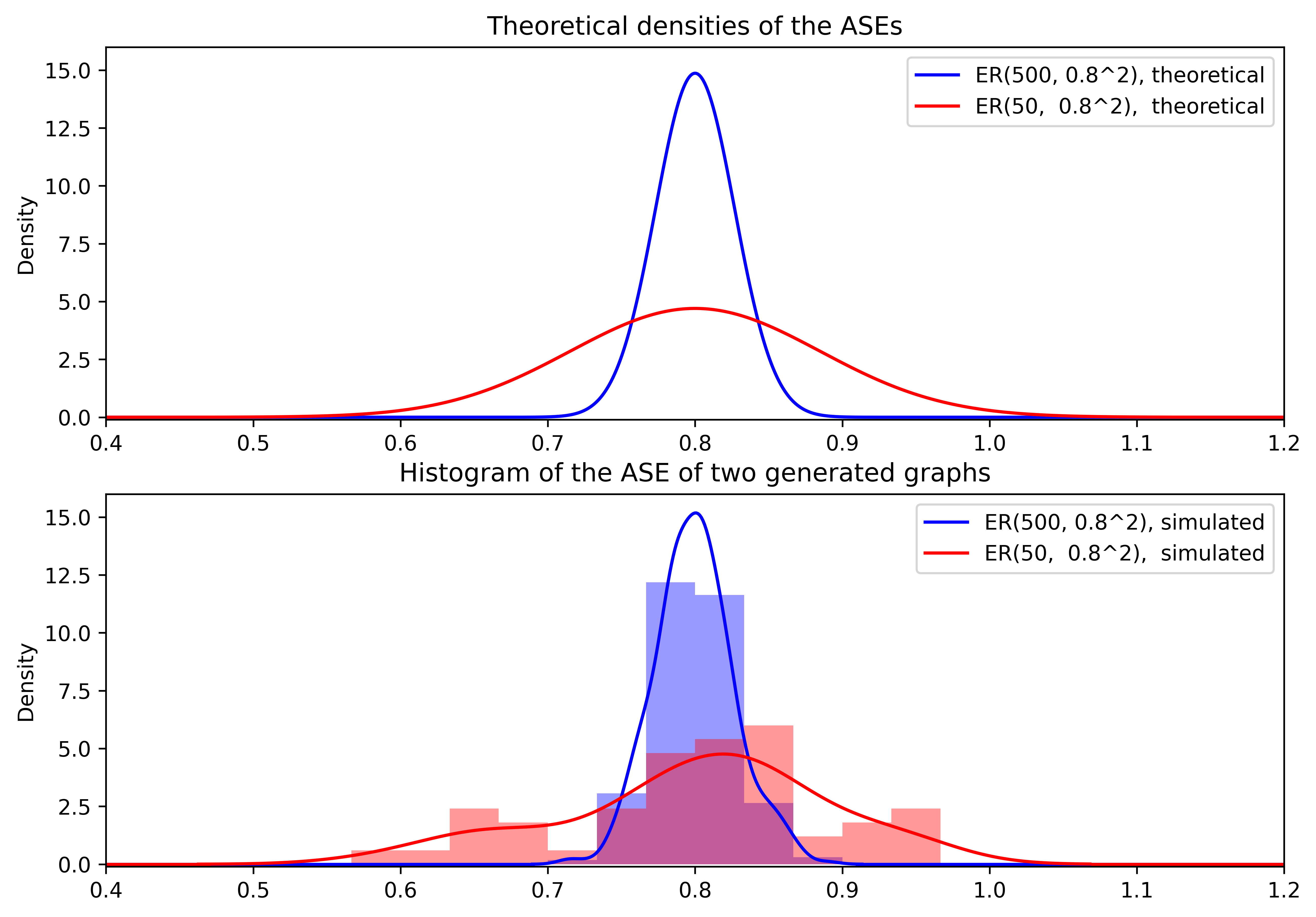
Figure 2: A visualization of the ASEs for the Erdös-Rényi graphs with the same edge probability, but vastly different orders. Top: theoretical densities of the ASEs; bottom: the histogram of the ASEs of two generated graphs, with kernel density estimates.

Consider the following simple example. Suppose that the graphs have distributions $\boldsymbol{A}\sim ER(n,p^{2})$ and $\boldsymbol{B}\sim ER(m,p^{2})$. Then, the distributions of the ASEs become

$$\hat{\boldsymbol{X}}_{i}\overset{approx}{\sim}\mathcal{N}\left(p,\frac{1-p^{2}}{n}\right)\quad\mathrm{and}\quad\hat{\boldsymbol{Y}}_{i}\overset{approx}{\sim}\mathcal{N}\left(p,\frac{1-p^{2}}{m}\right).$$ (4)

up to an orthogonal nonidentifiablity, which in a single dimension is just a sign flip.

A visualization of this specific case with parameters $n=500,m=50$, and $p=0.8$ is provided in Figure 2. The ASEs have substantially different distributions from each other, despite the identical distributions of the true latent positions. As will be demonstrated in Section 4, in this case the nonparametric test developed by Gretton et al. (2012) and employed by Tang et al. (2017) rejects more often than the significance level $\alpha$, as it should.

Indeed, the test of Gretton et al. (2012) cannot be used directly on the adjacency spectral embeddings of two graphs of different order to test for the equivalence of the distributions of the latent positions, as it is not valid.

3.2 Corrected adjacency spectral embeddings

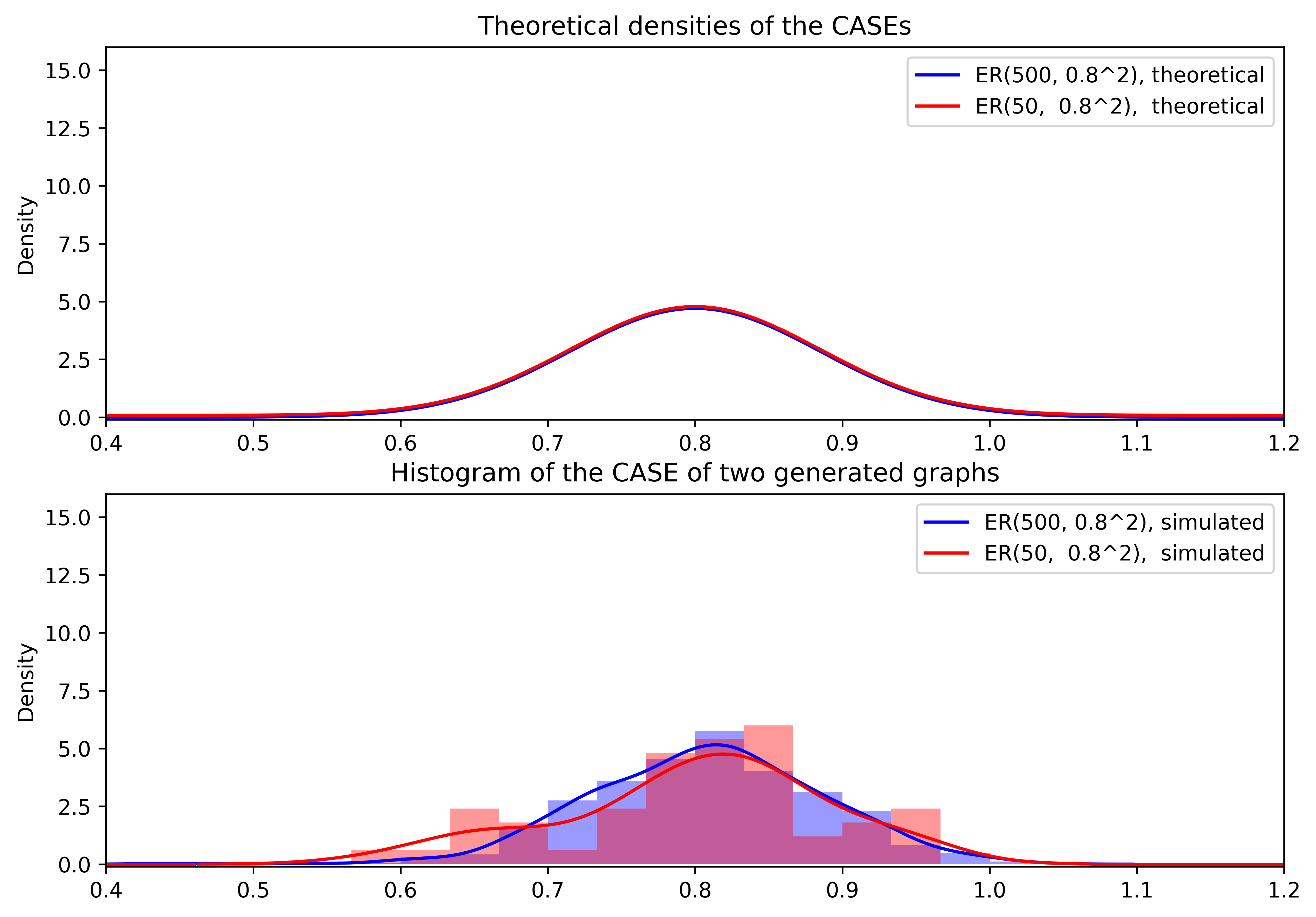
Figure 3: A visualization of the CASEs for the Erdös-Rényi graphs with the same edge probability, but vastly different orders. Top: theoretical densities of the corrected ASEs; bottom: the histogram of the corrected ASEs of two generated graphs, with kernel density estimates.

We propose modifying the adjacency spectral embeddings of one of the graphs by injecting appropriately scaled Gaussian noise. The noise inflates the variances of the ASE of the larger graph to approximately the same value as the smaller graph and makes the latent positions exchangeable under the null hypothesis.

Definition 8 (Corrected Adjacency Spectral Embedding).

Consider two $d$-dimensional random dot product graphs $(\boldsymbol{A},\boldsymbol{X})\sim RDPG(F,n)$ and $(\boldsymbol{B},\boldsymbol{Y})\sim RDPG(G,m)$. Without loss of generality, assume that $n>m$. For every row in the adjacency spectral embedding of the larger graph, $\hat{\boldsymbol{X}}_{i}$, consider estimating its variance using the plug-in estimator from Equation 2, and then sampling a point $\boldsymbol{\epsilon}_{\hat{\boldsymbol{X}}_{i}}\sim\mathcal{N}(\mathbf{0},\left(\frac{1}{m}-\frac{1}{n}\right)\hat{\boldsymbol{\Sigma}}(\hat{\boldsymbol{X}}_{i}))$. For every row in the adjacency spectral embedding of the smaller graph, $\hat{\boldsymbol{Y}}_{j}$, define $\boldsymbol{\epsilon}_{\hat{\boldsymbol{Y}}_{j}}:=\mathbf{0}$. Let $\widetilde{\boldsymbol{X}}_{i}=\hat{\boldsymbol{X}}_{i}+\boldsymbol{\epsilon}_{\hat{\boldsymbol{X}}_{i}}$ for all $i$ and $\widetilde{\boldsymbol{Y}}_{j}=\hat{\boldsymbol{Y}}_{j}+\boldsymbol{\epsilon}_{\hat{\boldsymbol{Y}}_{j}}$ for all $j$. We denote the matries whose rows consist of these new vectors $\widetilde{\boldsymbol{X}}$ and $\widetilde{\boldsymbol{Y}}$, respectively, and we call them the corrected adjacency spectral embeddings (CASE). The corrected adjacency spectral embeddings of two graphs of the same order are equal to the standard adjacency spectral embeddings.

The motivation for the preceding definition is as follows. Recall that we have assumed without the loss of generality that $n>m$. Conditioned on the true latent positions, the rows of the corrected adjeacency spectral embeddings have distributions that are given by

$$\widetilde{\boldsymbol{X}}_{i}|\boldsymbol{X}_{i} \overset{approx}{\sim}\mathcal{N}\left(\boldsymbol{X}_{i}\boldsymbol{W}_{\boldsymbol{X}},\frac{\boldsymbol{\Sigma}(\boldsymbol{X}_{i})}{n}+\left(\frac{1}{m}-\frac{1}{n}\right)\hat{\boldsymbol{\Sigma}}(\hat{\boldsymbol{X}}_{i})\right)$$ (5)

$$\widetilde{\boldsymbol{Y}_{i}}|\boldsymbol{Y}_{i} \overset{approx}{\sim}\mathcal{N}\left(\boldsymbol{Y}_{i}\boldsymbol{W}_{\boldsymbol{Y}},\frac{\boldsymbol{\Sigma}(\boldsymbol{Y}_{i})}{m}\right).$$

Unlike Equation 3, these distributions are approximately the same, up to orthogonal transformations $\boldsymbol{W}_{\boldsymbol{X}}$ and $\boldsymbol{W}_{\boldsymbol{Y}}$. This is true regardless of the ratio of graph orders, as long the true latent positions $\boldsymbol{X}_{i},\boldsymbol{Y}_{i}$ have the same distribution and $\hat{\boldsymbol{\Sigma}}$ is a good estimator of $\boldsymbol{\Sigma}$. As an illustrative example, we revisit the ER ilustration from the previous section. A visualization of the theoretical and simulated CASEs of two ER graphs with vastly different orders is presented in Figure 3. Both the theoretical and the simulated corrected embeddings have the same distribution. Hence, the corrected adjacency spectral embeddings can be used as inputs to the latent distribution test of Tang et al. (2017).

We note that due to the exact equivalence of the maximum mean discrepancy test of Gretton et al. (2012), the Energy distance two-sample test Székely and Rizzo , the Hilbert-Schmidt independence criterion (Gretton et al., 2007), and distance correlation (Székely et al., 2007; Székely and Rizzo, 2014) test for independence, any of these four can be used as a subsequent test interchangeably (Shen and Vogelstein, 2021; Panda et al., 2021). In the case of the latter two of the four, one first has to concatenate the two embeddings, define an auxiliary label vector, and then perform the independence test. For more on this procedure, sometimes called $k$-sample transform, see Shen and Vogelstein (2021).

It may also be possible to use other independence tests framed as two-sample tests to test for the equivalence of the latent distributions after the embeddings have been obtained and corrected. Such tests include, but are not limited to RV (Escoufier, 1973; Robert and Escoufier, 1976) which is the multivariate generalization of the Pearson correlation (Pearson, 1895), canonical component analysis (Hardoon et al., 2004), and multiscale graph correlation (Lee et al., 2019; Shen et al., 2020). The power of the multiscale graph correlation against some alternatives has been studied in the graph setting in Chung et al. (2022). However, no theoretical guarantees, at least known to us, have been established in the graph setting for any of these tests.

4 Simulation study

We conduct a simulation study comparing the latent distribution tests that use regular and corrected ASEs. We use graphs generated from the ER, SBM and RDPG models in our experiments. However, we always estimate the variances of the ASE using the generic plug-in estimator for the RDPG model, provided in Equation 2. That is, we do not use the knowledge that the latent distribution is truly a point-mass, or a mixture thereof, anywhere in our experiments.

The implementation of the latent distribution test used in this simulation study is incorporated into graspologic (Chung et al., 2019) Python package, both for ASE and CASE. This implementation exploits the exact equivalence with independence tests described above. Code that is compatible with the latest version of graspologic and can be used to reproduce all of the simulations is available at https://github.com/alyakin314/correcting-nonpar.

We set the number of permutations used to generate the null distribution to 200. For a task like this, it is quite common to use a gaussian kernel with a bandwith selected using a median heuristic (Garreau et al., 2017), which in practice might be more sensetive than most arbitrarily chosen constant bandwidths. However since the theoretical result holds only a fixed kernel, we chose to use a Gaussian kernel with a fixed bandwidth $\sigma=0.5$ throughout our experiments.

4.1 Erdös-Rényi Graphs: Validity and Consistency

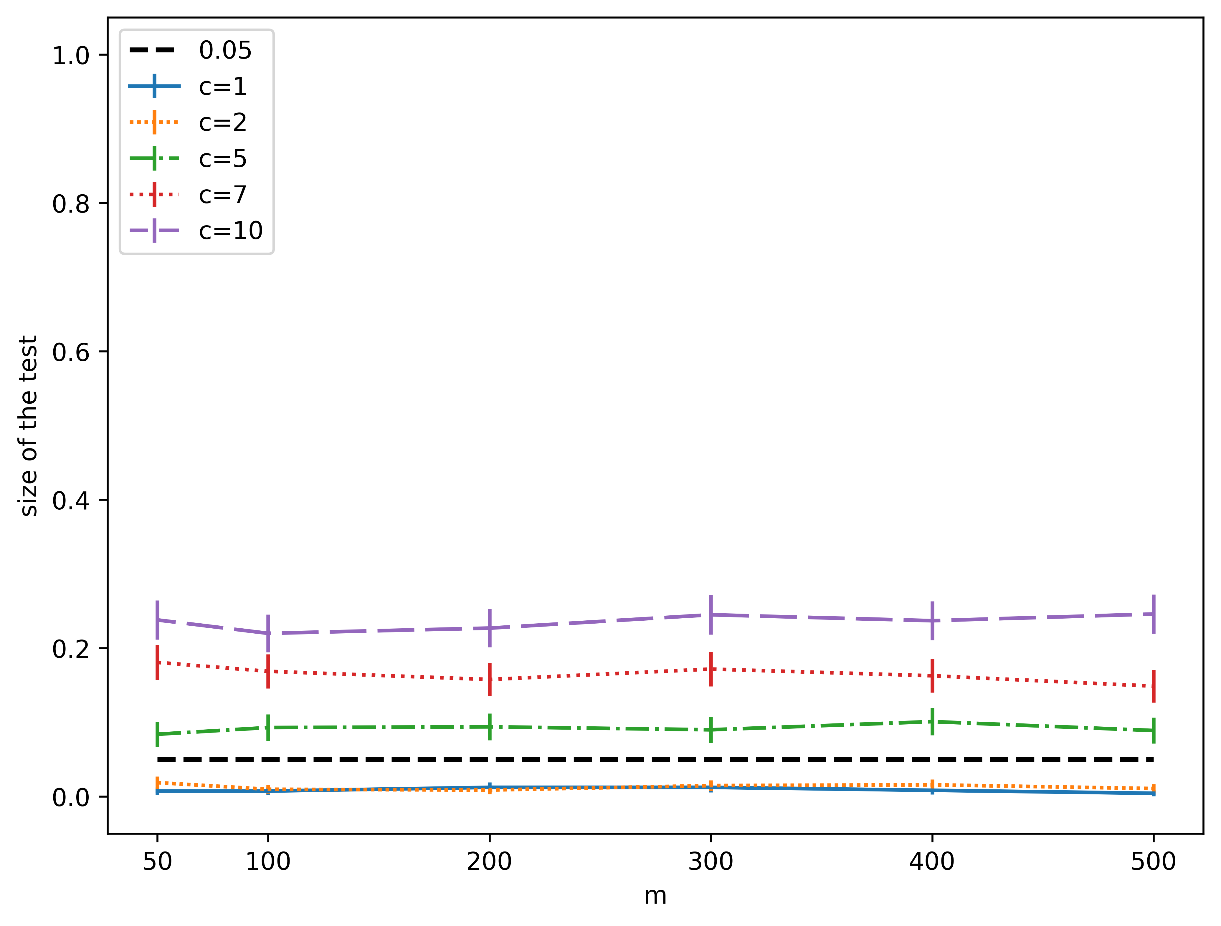
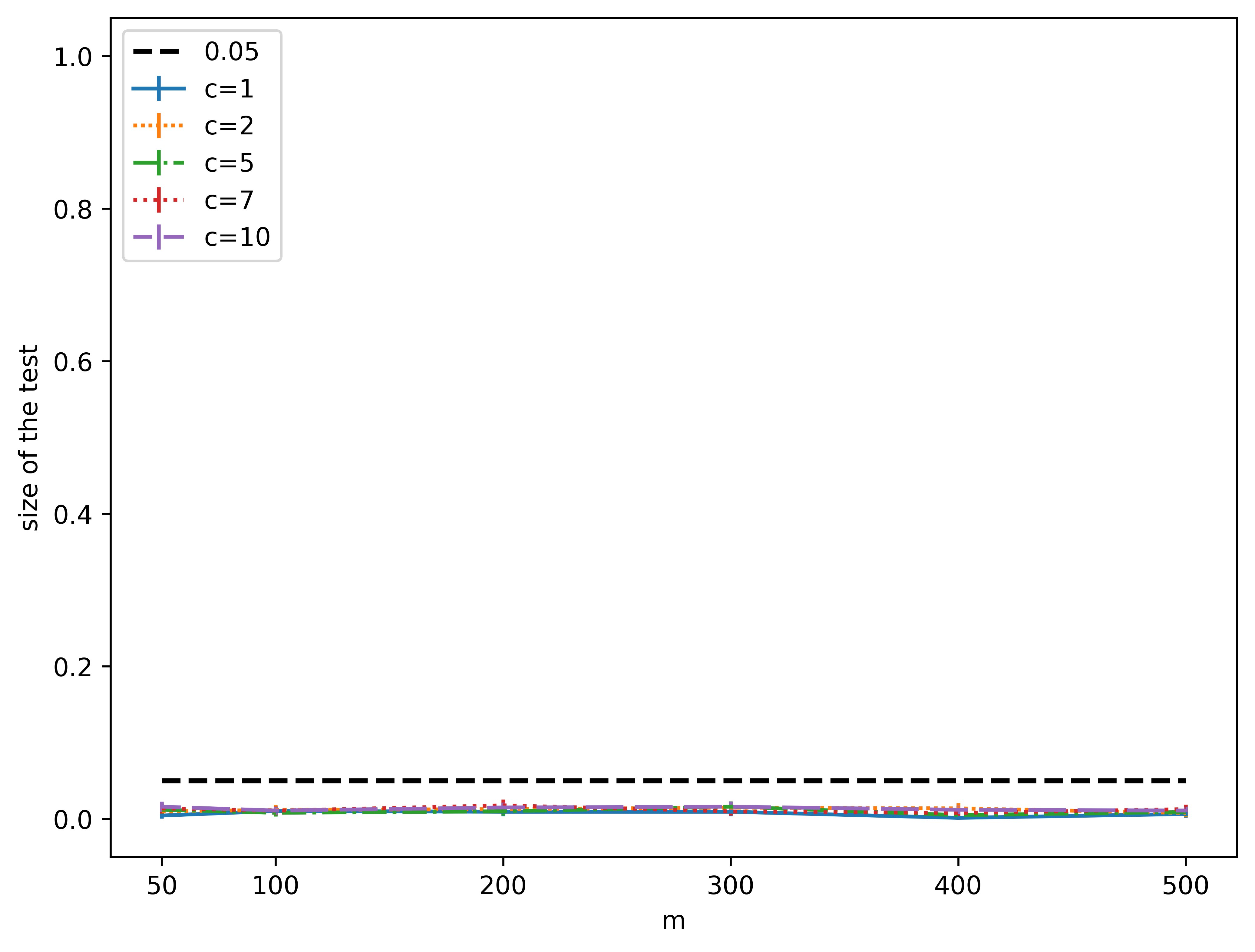
Figure 4: Size of the nonparametric latent distribution permutation tests that use the standard ASE (left) and the CASE (right). Graphs are $\boldsymbol{A}\sim ER(n,0.8^{2})$ and $\boldsymbol{B}\sim ER(cn,0.8^{2})$. Error bars represent 95% confidence interval.

We generate pairs of graphs from the null hypothesis of the test: $\boldsymbol{A}\sim ER(n,p^{2})$ and $\boldsymbol{B}\sim ER(m,p^{2})$ with $m=cn$. We consider different ratios of the graphs orders $c\in\{1,2,5,7,10,\}$, and different smaller graph orders $n\in\{50,100,200,300,400,500\}$. We use the latent position $p=0.8$, which corresponds to the Erdös-Rényi graphs with the edge probability of $0.64$. We always embed the graphs into one dimension and we overcome orthogonal nonidentifiability by flipping the signs of the ASE of a graph if their median is negative. $1000$ Monte-carlo replications are used for each of combination of $c$ and $n$ tested.

We set $\alpha$ to $0.05$ and report the sizes of the test in Figure 4. The size of the test that use the standard ASE grows as a function of $c$ rendering it invalid for graphs of different sizes. The size of the test that uses the CASE remains below $0.05$ across all choices of $c$ and $n$ considered.

In general, the size of the permutation tests should be exactly $\alpha$. However, due to the intricate dependence behavior of the graph spectral embeddings (Athreya et al., 2016; Tang et al., 2022), the tests ends up being conservative. The extent to which the test is conservative is dependent on the model from which the graphs were generated, and thus cannot be easily corrected. The scope of this work is limited to correcting the invalidity phenomenon and not the conservatism of this test.

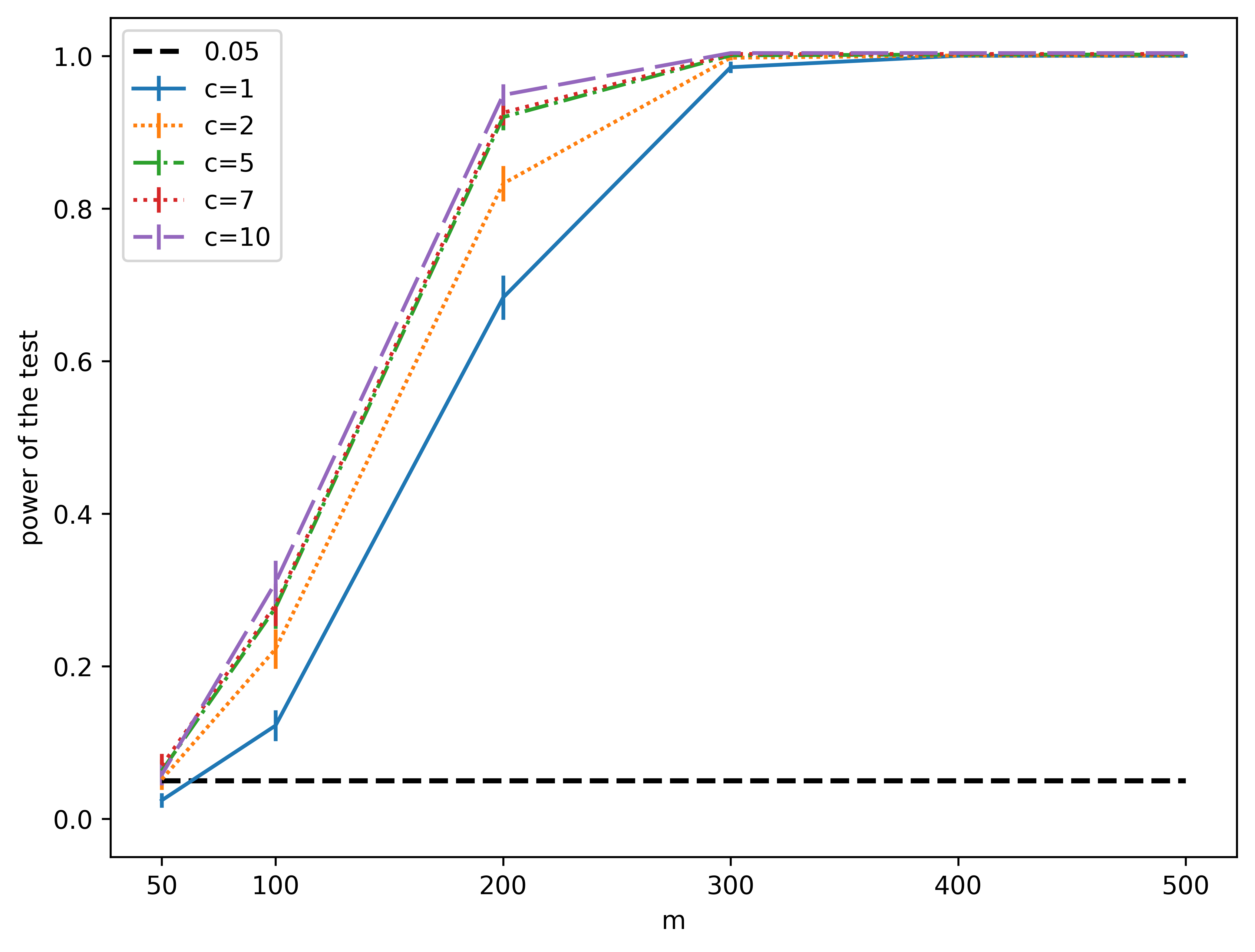
Figure 5: Power of the nonparametric latent distribution permutation test that uses CASE against the alternative with graphs generated from $\boldsymbol{A}\sim ER(n,0.8^{2})$ and $\boldsymbol{B}\sim ER(cn,0.79^{2})$. Error bars represent 95% confidence interval.

We also study the behavior of the test under the alternative hypothesis in order to assess its power. We use the alternative hypothesis $\boldsymbol{A}\sim ER(n,p^{2})$ and $\boldsymbol{B}\sim ER(m,q^{2})$, with $p=0.8$ and $q=0.79$ and $m=cn$ for various ratios $c$. We again consider the graph order ratios $c\in\{1,2,5,7,10\}$, and smaller graph orders $n\in\{50,100,200,300,400,500\}$. For $c=1$, CASE overlaps exactly with the standard ASE, so the testing procedure is the same as the original test of Tang et al. (2017). For all other choices of $c$, the original test is not valid, and is thus omitted from study.

The results of this study are presented in Figure 5. The power of the test goes to one as the sample size increases for all choices of $c$ used, which suggests that the test that uses CASE is still consistent. We note that for any given $n$, the power of the test grows as $c$ grows; this behavior is expected, since the number of vertices in one graph is held constant and the number of vertices in the other increases, so the total number of observations grows.

4.2 Stochastic Block Model Graphs: Higher Dimensions

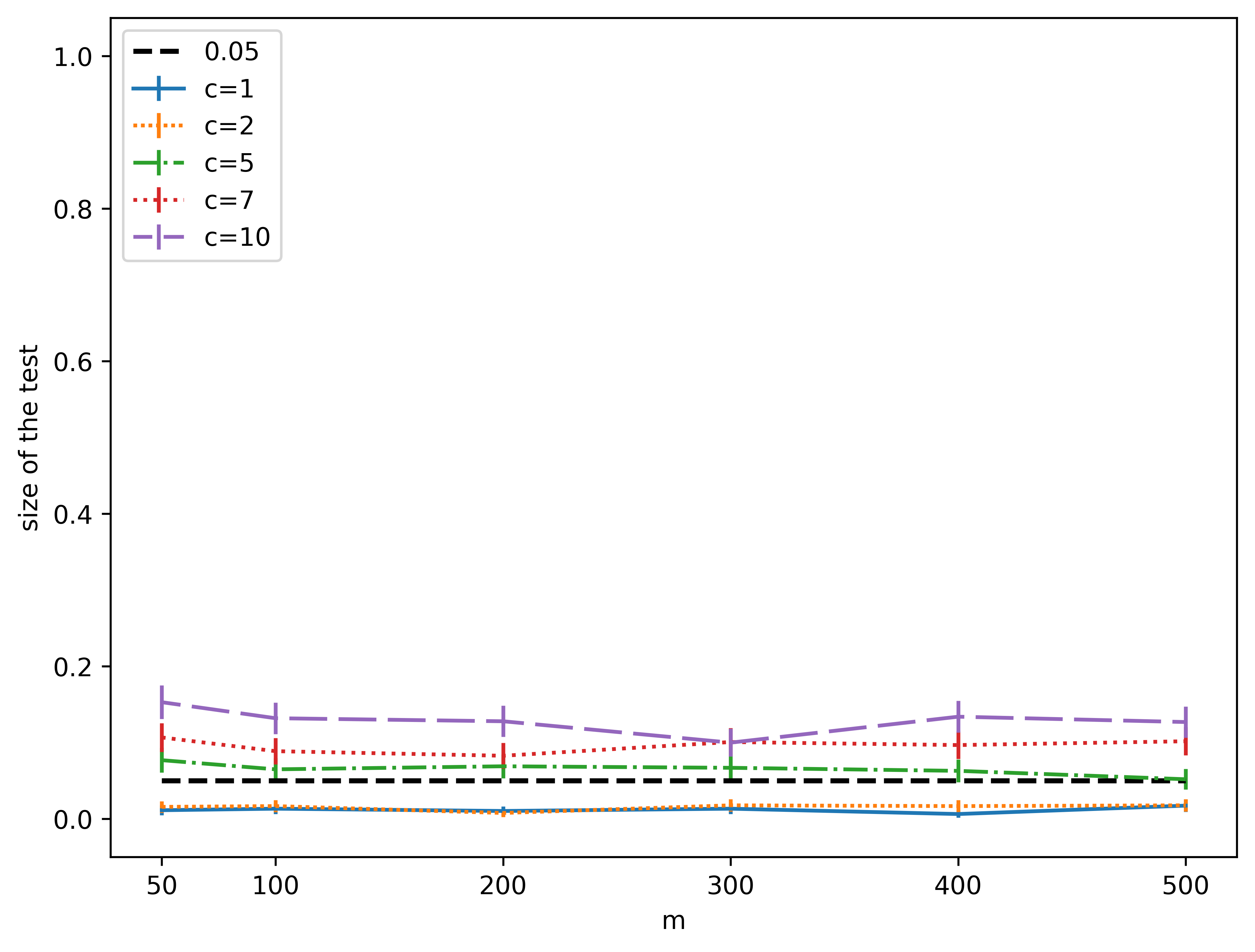
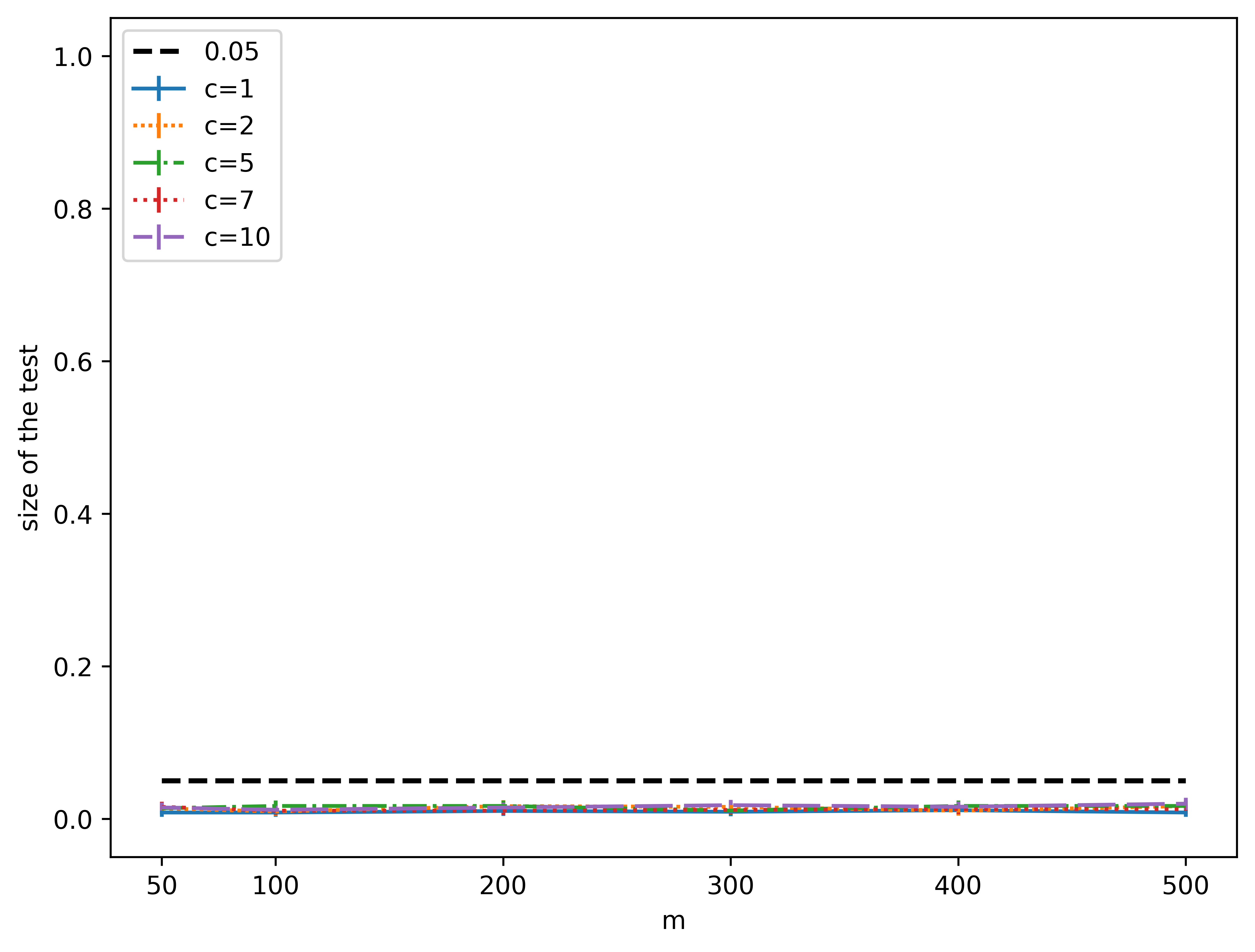
Figure 6: Size of the nonparametric latent distribution permutation tests that use the regular ASE (left) and the CASE (right). Graphs are $\boldsymbol{A}\sim SBM(n,\boldsymbol{\pi},\boldsymbol{P})$ and $\boldsymbol{B}\sim SBM(cn,\boldsymbol{\pi},\boldsymbol{P})$. Error bars represent 95% confidence interval.

We repeat the validity and consistency experiments, but use $3$-block SBMs, instead of ER graphs. In all simulations we use the vector of prior probabilities $\boldsymbol{\pi}=[0.4,0.3,0.3]^{T}$. To estimate size, we use graphs $\boldsymbol{A}\sim SBM(n,\boldsymbol{\pi},\boldsymbol{P})$ and $\boldsymbol{B}\sim SBM(m,\boldsymbol{\pi},\boldsymbol{P})$, where the block-probability matrix $\boldsymbol{P}=\boldsymbol{Z}\boldsymbol{Z}^{T}$ is obtained using the matrix of latent positions $\boldsymbol{Z}$ is being parametrized by spherical coordinates

$$\boldsymbol{Z} =\begin{bmatrix}\begin{bmatrix}r\sin(\boldsymbol{\theta}_{1})\sin(\boldsymbol{\omega}_{1})\\ r\sin(\boldsymbol{\theta}_{1})\cos(\boldsymbol{\omega}_{1})\\ r\cos(\boldsymbol{\theta}_{1})\end{bmatrix},\begin{bmatrix}r\sin(\boldsymbol{\theta}_{2})\sin(\boldsymbol{\omega}_{2})\\ r\sin(\boldsymbol{\theta}_{2})\cos(\boldsymbol{\omega}_{2})\\ r\cos(\boldsymbol{\theta}_{2})\end{bmatrix},\begin{bmatrix}r\sin(\boldsymbol{\theta}_{3})\sin(\boldsymbol{\omega}_{3})\\ r\sin(\boldsymbol{\theta}_{3})\cos(\boldsymbol{\omega}_{3})\\ r\cos(\boldsymbol{\theta}_{3})\end{bmatrix}\end{bmatrix}^{T},$$

where $r=0.9$, $\boldsymbol{\theta}=[0,0.2,0.4,0.5]^{T}$, and $\boldsymbol{\omega}=[0.00,0.10,0.05,0.05]^{T}$ (the fourth coordinate will become relevant for the evaluation of power). Numerically,

$$\boldsymbol{Z} \approx\begin{bmatrix}\begin{bmatrix}0.000\\ 0.000\\ 0.900\end{bmatrix},\begin{bmatrix}0.018\\ 0.178\\ 0.882\end{bmatrix},\begin{bmatrix}0.018\\ 0.350\\ 0.829\end{bmatrix}\end{bmatrix}^{T}$$

and

$$\boldsymbol{P} \approx\begin{bmatrix}0.810&0.794&0.746\\ 0.794&0.810&0.794\\ 0.746&0.794&0.810\end{bmatrix}.$$

Exactly as the one-dimensional case, we constrain $m=cn$ and consider the graph order ratios $c\in\{1,2,5,7,10\}$, and smaller graph orders $n\in\{50,100,200,300,400,500\}$. We always embed into the true dimension $d=3$. We overcome orthogonal nonidentifiability by aligning the medians of the embeddings to be in the same quadrant by flipping all of the signs on one of them if they do not match. The size of the tests at $\alpha=0.05$ is presented in Figure 6. Similarly to the one-dimensional setting, the size of the test that uses standard ASE grows as a function of $c$, but is unaffected for the test that uses CASE.

Figure 7: Power of the nonparametric latent distribution permutation test that uses CASE against the alternative with graphs generated from $\boldsymbol{A}\sim SBM(n,\boldsymbol{\pi},\boldsymbol{P})$ and $\boldsymbol{B}\sim SBM(m,\boldsymbol{\pi},\boldsymbol{P}^{\prime})$,. Error bars represent 95% confidence interval.

To estimate power and demonstrate consistency in higher dimensions we use a pair of graphs $A$ and $B$, generated from $SBM(n,\boldsymbol{\pi},\boldsymbol{P})$ and $SBM(m,\boldsymbol{\pi},\boldsymbol{P}^{\prime})$, respectively, where $\boldsymbol{P}$ is as defined above, and $\boldsymbol{P^{\prime}}=\boldsymbol{Z^{\prime}}\boldsymbol{Z^{\prime}}^{T}$ with

$$\boldsymbol{Z^{\prime}} =\begin{bmatrix}\begin{bmatrix}r\sin(\boldsymbol{\theta}_{1})\sin(\boldsymbol{\omega}_{1})\\ r\sin(\boldsymbol{\theta}_{1})\cos(\boldsymbol{\omega}_{1})\\ r\cos(\boldsymbol{\theta}_{1})\end{bmatrix},\begin{bmatrix}r\sin(\boldsymbol{\theta}_{2})\sin(\boldsymbol{\omega}_{2})\\ r\sin(\boldsymbol{\theta}_{2})\cos(\boldsymbol{\omega}_{2})\\ r\cos(\boldsymbol{\theta}_{2})\end{bmatrix},\begin{bmatrix}r\sin(\boldsymbol{\theta}_{4})\sin(\boldsymbol{\omega}_{4})\\ r\sin(\boldsymbol{\theta}_{4})\cos(\boldsymbol{\omega}_{4})\\ r\cos(\boldsymbol{\theta}_{4})\end{bmatrix}\end{bmatrix}^{T}.$$

Numerically,

$$\boldsymbol{Z^{\prime}} \approx\begin{bmatrix}\begin{bmatrix}0.000\\ 0.000\\ 0.900\end{bmatrix},\begin{bmatrix}0.018\\ 0.178\\ 0.882\end{bmatrix},\begin{bmatrix}0.022\\ 0.431\\ 0.790\end{bmatrix}\end{bmatrix}^{T}$$

and

$$\boldsymbol{P^{\prime}} \approx\begin{bmatrix}0.810&0.794&0.711\\ 0.794&0.810&0.774\\ 0.711&0.774&0.810\end{bmatrix}.$$

Note that the only differing feature of the second graph is the latent position of the vertices in the third block, and the difference is entirely explained by the position being slightly further away in the $\theta$ coordiante. The graph orders and ratios of thereof are identical to the ones used in the validity simulation. The results are presented in the Figure 7. The test that uses the CASE remains consistent even in $d=3$.

4.3 Random Dot Product Graphs: General Setting

Figure 8: Density / Mass functions visualization for $F_{x}=0.3\ Uniform(0,1)+0.3,F_{y}=0.3\ Beta(0.25,0.25)+0.3$, and $F_{z}=0.3\ Bernoulli(0.5)+0.3$. All three are used as latent position distributions in our experiments.

Lastly, we present a simulation with continious latent distributions. Specifically, consider three different distributions:

$$F_{x} =0.3\ Uniform(0,1)+0.3$$

$$F_{y} =0.3\ Beta(0.25,0.25)+0.3$$

$$F_{z} =0.3\ Bernoulli(0.5)+0.3$$

Note that all three distributions can be formulated in the context of the $0.3\ Beta(a,a)+0.3$ model. Namely, $F_{x}$ is equivalent to $0.3\ Beta(1,1)+0.3$, $F_{y}$ is in such a form already, and $0.3\ Beta(a,a)+0.3\to F_{z}$ as $a\to 0$. $F_{y}$ can be thought of as an intermediate step between the $F_{x}$ and $F_{z}$. The visualizations of the density or mass functions of these distributions are provided in Figure 8.

Also, observe that $F_{z}$ is nothing more than the latent distribution of a two-block SBM in a single dimension with a block-probability matrix

$$\boldsymbol{P} =\begin{bmatrix}0.6^{2}&(0.6)(0.3)\\ (0.3)(0.6)&0.3^{2}\end{bmatrix},$$

whereas $F_{x}$ and $F_{y}$ can be thought as latent distributions of either DCSBMs or MMSBMs, as per Remark 4. Thinking of them as MMSBMs with $\boldsymbol{Z}=[0.6,0.3]^{T}$, the parameter $a$ can be viewed as a mixing coefficient: $F_{x}$ has a lot of mixing, $F_{y}$ has some mixing, and $F_{z}$ has two components completely separated.

Figure 9: Size of the nonparametric latent distribution permutation tests that use the regular ASE (left) and the CASE (right). Graphs are $\boldsymbol{A}\sim RDPG(F,n)$ and $\boldsymbol{B}\sim RDPG(F,m)$, where $F\in\{F_{x},F_{y},F_{z}\}$. Error bars represent 95% confidence interval.

First, we consider graphs $\boldsymbol{A}$ and $\boldsymbol{B}$ generated from $(\boldsymbol{X},\boldsymbol{A})\sim RDPG(F,n)$, and $(\boldsymbol{Y},\boldsymbol{B})\sim RDPG(F,m)$, with $m=cn$ This setting is in the null hypothesis of the latent distribution test. Unlike the previous experiment settings, we set $c$ to a single value of $10$, and instead vary the distributions of the latent positions. We consider $F\in\{F_{x},F_{y},F_{z}\}$. The number of vertices of the smaller graph, $n$, is once again varied to be $\{50,100,200,300,400,500\}$. We generate 1000 pairs of graphs for each of the possible settings, and use both a test that uses ASE and a test that uses CASE. Like before, we overcome orthogonal nonidentifiability by aligning the medians of the embeddings via flippting signs.

Results of this simulation are presented in the Figure 10. Observe that the test that uses ASE is not valid for all three distributions of the latent positions, which is especially clear at the small $n$. On the other hand - test that uses CASE remains experimentally valid for all three distributions: with no mixing, little mixing, and a lot of mixing.

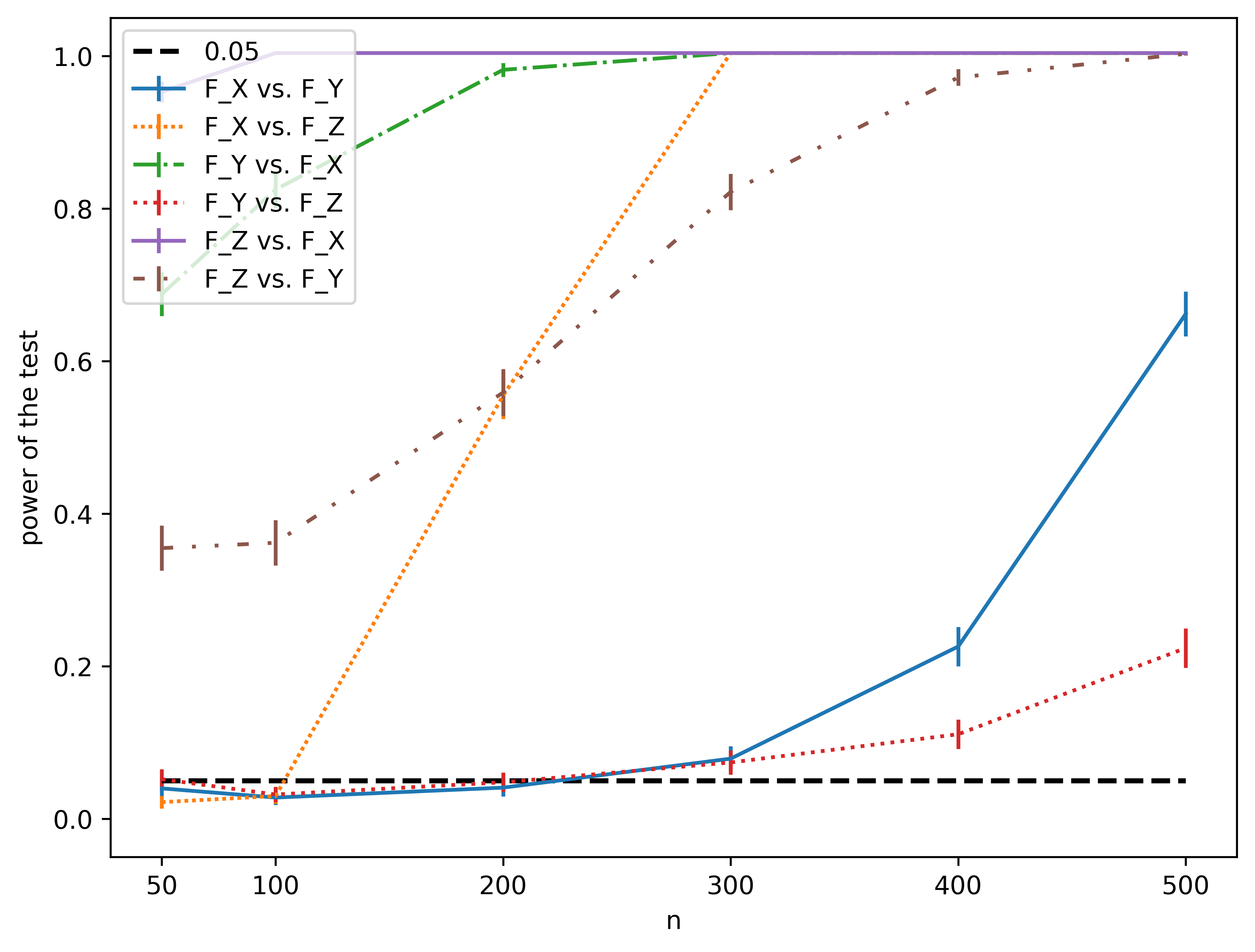
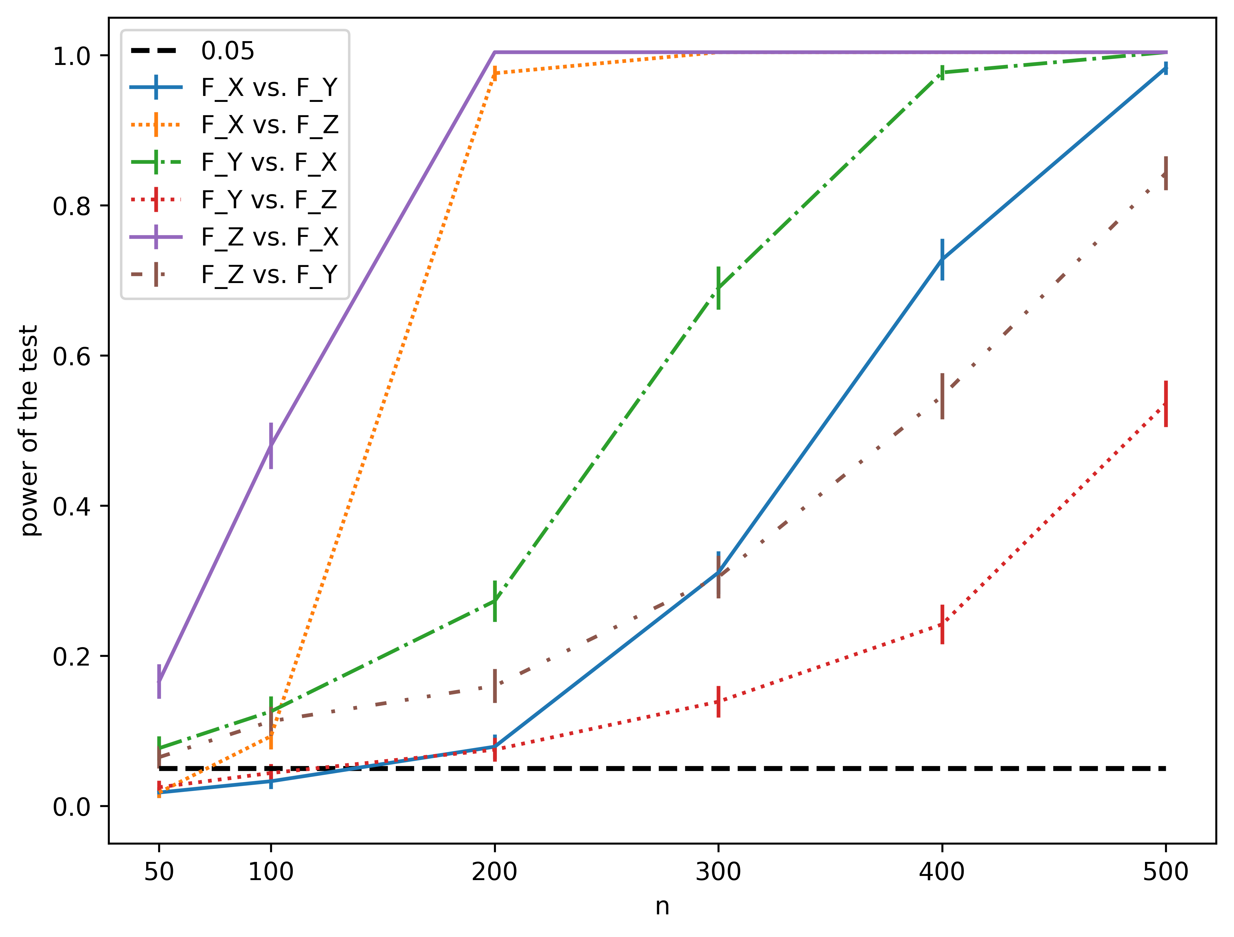
Figure 10: Power of the nonparametric latent distribution permutation tests that use the regular ASE (left) and the CASE (right). Graphs are $\boldsymbol{A}\sim RDPG(F_{1},n)$ and $\boldsymbol{B}\sim RDPG(F_{1},m)$, where $(F_{1},F_{2})\in\{F_{x},F_{y},F_{z}\}\times\{F_{x},F_{y},F_{z}\}$, except for the cases when $F_{1}=F_{2}$, as those are presented in Firgure 9. Error bars represent 95% confidence interval.

Next, we simulate the power of the test under different alternatives. Specifically, we generate pairs of graphs $\boldsymbol{A}$ and $\boldsymbol{B}$, where $(\boldsymbol{X},\boldsymbol{A})\sim RDPG(F,n)$, and $(\boldsymbol{Y},\boldsymbol{B})\sim RDPG(F^{\prime},m)$, where $m=cn$. We keep the same settings of $n$ and $c$ as for the study of the test size, and pick $(F,F^{\prime})$ from the collection $\{F_{x},F_{y},F_{z}\}\times\{F_{x},F_{y},F_{z}\}$, excluding the cases where $F=F^{\prime}$, as those have been studied previously, and are not under the alternative. Note that the ordering within the pair matters, because the two graphs are not of the same order. We generate $1000$ graphs for each of the possible combination of of $F$, $F^{\prime}$, $c$, and $n$. We embed the graphs in one dimension using ASE or CASE, use orthogonal alignment via the median trick, and perform the nonparametric test. Previously, we were omitting the power simulation that uses the invalid version of the test, since a test that doesn’t need to be valid can be arbitrarily powerful (simply, consider a test that always rejects). However, we include the results here because they demonstrate an important point regarding the using the uncorrected verions of the test.

The power of the test at significance level $\alpha=0.05$ in these six possible settings is summarized in Figure 10. There are several important observations we can make. First, consider the right pannel which summarizes the emperical power of the test that uses CASE. The power monotonically increases as $n$ grows, hence the test for the latent distribution that uses CASE is able to meaningfully distinguish between MMSBMs with different amounts of mixing. Furthermore, observe that the settings of $F_{x}$ vs. $F_{z}$ and $F_{z}$ vs. $F_{x}$, have more power than the all over ones. Thus, the power in the setting when one mixture has a lot of mixing and the other has no mixing at all is larger than the power in the setting of no versus some mixing, or in the setting with some versus a lot of mixing, as one would expect.

Next, consider the left pannel, which presents the power using the invalid version of the test that uses ASE. Observe that for some settings the power decreases when using the corrected version of the test decreases, but increases for others. In particular, it decreases the for settings of $F_{y}$ vs. $F_{x}$, $F_{z}$ vs. $F_{x}$, and $F_{z}$ vs. $F_{y}$, and increases for the settings of $F_{x}$ vs. $F_{y}$, $F_{x}$ vs. $F_{y}$, and $F_{y}$ vs. $F_{z}$. To summarize, power decreases in the cases when the smaller graph has more mixing than the larger graph, and increases when the smaller graph has less mixing. Our conjecture is that the increase of in power with the correction can happen if the distribution of the latent positions of the smaller graph has smaller variance, as happens in the cases where the smaller graph has more mixing. In over words, the difference in variance due to the inherent differences in latent distributions is partially compensated by the difference in variance due to estimation, which leads to less powerful test if the correction is not used. Thus, using the uncorrected version of the test can both lead to incorrect inference under the null hypothesis, and a less sensitive inference under some alternatives.

5 Real World Application

We demonstrate an application of this testing procedure to a real world dataset of human connectomes. A connectome, also known as a brain graph (Chung et al., 2021), represents the brain as a network with neurons (or collections thereof) as vertices, and synapses (or structural connections) as edges. For this demonstration, the raw data is collected by diffusion magnetic resonance imaging (dMRI), which can represent the structural connectivity within the brain. (Yang et al., 2019) This example is predominantly included as an illustrative example of the applicability of the test to the setting and consistency of its results with a natural intuition. It should not be treated as an imaging study to draw conclusions about the dataset.

The macro-scale connectomes are estimated by NeuroData’s MRI to graphs (NDMG) pipeline (Kiar et al., 2018), which is designed to produce robust and biologically plausible connectomes across studies, individuals, and scans. The vertices of the graph represent regions of interest identified by spatial proximity, and the edges of the graph represent the connection between regions via tensor-based fiber streamlines. Specifically, there is an edge for a pair of regions if and only if there is a streamline passing between them. For more information on the procedure that generates the brain graphs, we refer the readers to Kiar et al. (2018). The data used in this study is the same one used by Yang et al. (2019).

Graphs in this dataset are weighted, directed, and have unknown dimension of the latent distribution. Thus, modifications to the procedure described in Subsection 2.3 are required to obtain the ASE of the graphs. The correction of ASE to CASE and the subsequent test are performed without further modifications. In addition to that, we do employ the median heuristic (Garreau et al., 2017) in order to determmine the bandwidth of the kernel. All of those modifications are implemented in graspologic (Chung et al., 2019) Python package, and, in fact, used by default whenever one uses a latent distribution test on a graphs that are directed, weighted, and/or have unspecified latent dimension.

There are 57 subjects in this dataset, each of which has 2 different dMRI scans. Furthermore, each of the scans was converted to a ’large’ and a ’small’ graph, using the aforementioned pipeline. The number of vertices in the large graphs varies between 730 and 1194, wheras the number of vertices in the small graphs varies between 493 and 814. We will refer to these large and small graphs as different scales. In this work all comparisons, whether within or between the subjects, take two graphs of different scales, one small and one large.

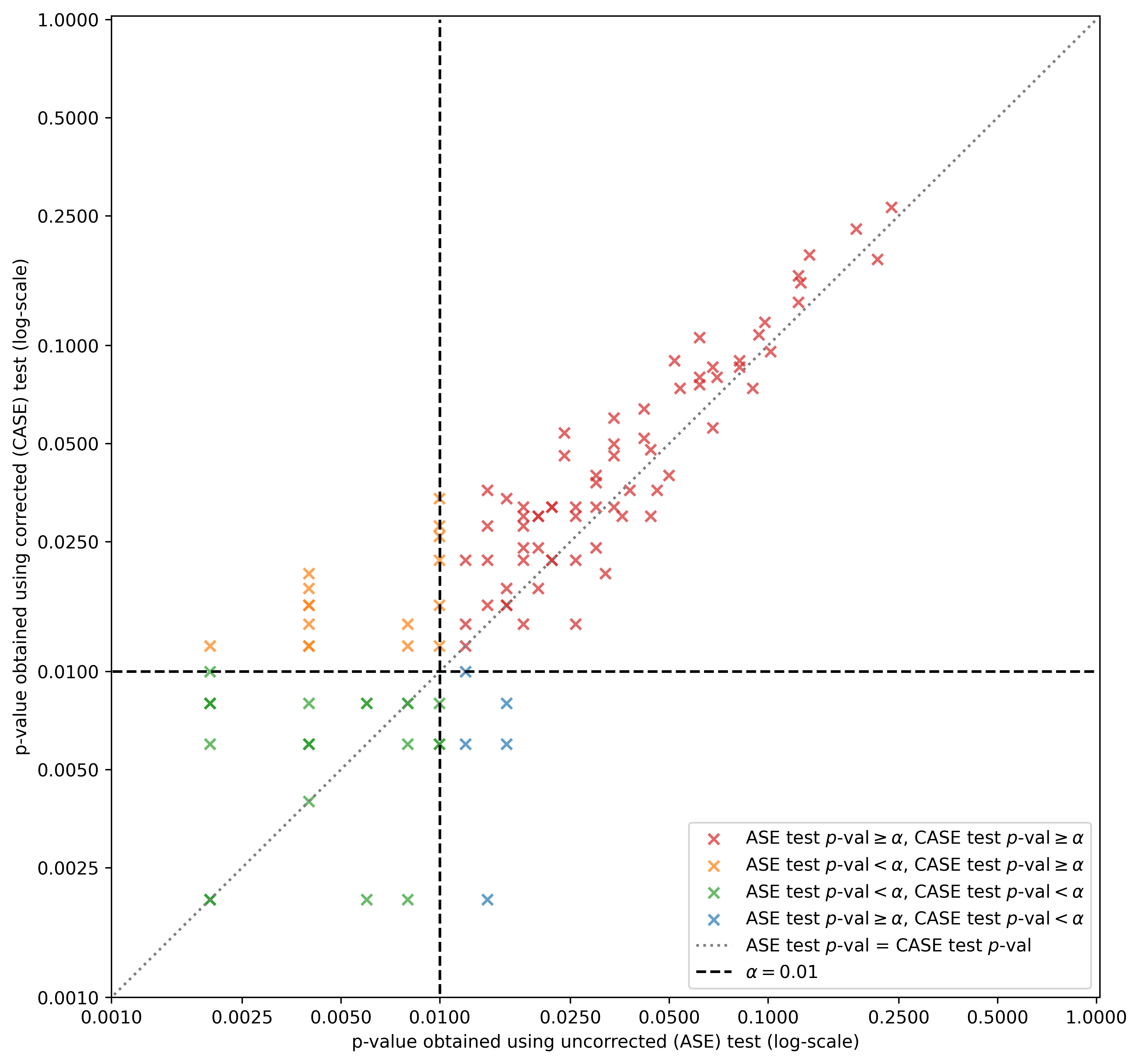
Figure 11: Comparison of the difference in $p$-values obtained using CASE and ASE in the setting of brain graphs of the same subject and scan but different scales. Color coding according to decision at $\alpha=0.01$. Note that some datapoints might overlap exactly due to permutation test providing a $p$-value from a discrete set.

We first use both the test that uses ASE and the test that uses CASE to compare the scans within the same subject, within the same scan, but between the two scales. There are 114 total possible comparisons. Paired differences in $p$-values obtained by the test that uses CASE and the test that uses ASE are presented in Figure 11. Using the one-sided Wilcoxon Signed-Rank test (Wilcoxon, 1945) on those pairs of $p$-values, we obtain $p$-value $<10^{-7}$, signifying that the corrected test rejects statistically less often than the uncorrected test.

We can furthermore consider decision-theoretic consequences by setting significance level $\alpha$ to two different commonly used values $0.01$ and $0.05$. In case of $\alpha=0.01$, both tests reject the null in 24 case, neither rejects in 69 cases, only ASE does in 16 cases, and only CASE does in just 5 cases (see color coding of Figure 11 but note that some data points overlap). Using the two-sided Fisher’s exact test, we obtain a statistic of 20.7 with a $p$-value $<10^{-8}$. Alternatively, setting $\alpha=0.05$, we obtain, a contigency table of: both: 89, none: 21, ASE only: 4, CASE only: 0, leading to a two-sided Fisher’s test statistic $p$-value $<10^{-18}$.

Thus, the test that uses CASE picks up the differences staistically less often when using both raw $p$-values and when using binary decisions by comparing $p$-values with significance levels $\alpha=\{0.01,0.05\}$. In Section 4.3 we demonstrated that using the uncorrected test can lead both to an invalid test under the null, and to a less sensitive test under some alternatives. Thus using a correction does not always imply having larger $p$-values. In this case, however, it does, which aligns with our natural intuition that a correct test should reject less often, as graphs obtained from the same scan but at different scales should be somewhat similar to each other.

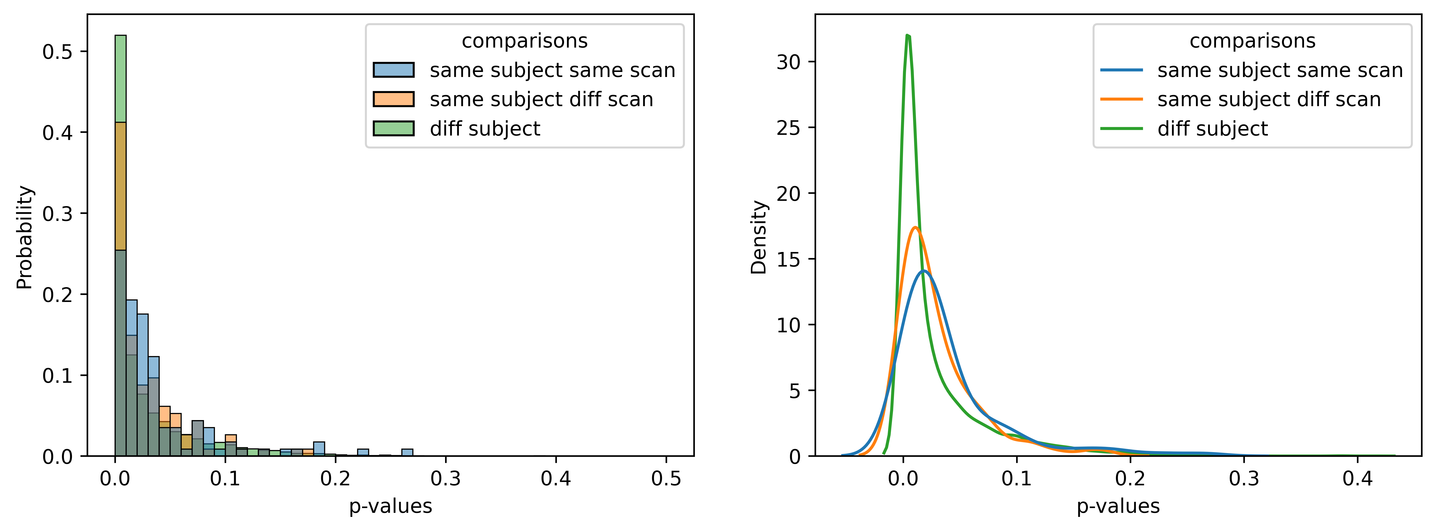
Figure 12: Comparison of the difference in $p$-values obtaind using CASE for different settings of the brain graph data. Left panel: Histograms of $p$-values with a bin size of 0.01. Normalized to add to 1. Right panel: Kernel density estiates of the distribution of $p$-values. Normalized to integrate to 1.

Next, we use the corrected test to compare the graphs between the scans and between subjects. Thre is a total of 114 possible comparisons in the setting of different scans of the same subject, as there are two comparisons per subject (larger scale scan 1 to smaller scale scan 2 and larger scale scan 2 to smaller scale scan 1) and 57 subjects total. For the case of different subject, there are $(57\times 2)\times(56\times 2)=12768$ total comparions (57 subjects each of which has 2 scans at larger scale compared to each of the 2 scans at smaller scale of everyone but themselves).

We plot the histograms and the kernel density estimates of the distribution of $p$-values, stratified by setting, in Figure 12. Using the one-sided ($>$) Mann-Whitney $U$ test (Mann and Whitney, 1947) we obtain: a $p$-value $0.020$ when comparing the distribution of $p$-values of the same subject within the scan to the distribution of $p$-values for the same subject between the scans, a $p$-value of $0.003$ when comparing the distribution of $p$-values of the same subject between the scans to the distribution of $p$-values between different subjects, and lastly, a $p$-value $<10^{-7}$ when comparing the distribution of $p$-values for the same subject within the scan to the distribution of $p$-values in the setting of different subjects.

To summarize, the $p$-values within the same subject same scan are smaller than within the same subject but different scan, which are themselves smaller than between different subjects. This aligns with the natural intuition that the test should reject more often for different scans than for the same scans and more often for the different subjects than for the same subjects.

6 Discussion

In this work we demonstrated that the latent distribution test proposed by Tang et al. (2017) degrades in validity as the numbers of vertices in two graphs diverge from each other. This phenomenon does not contradict the results of the original paper, as it occurs when test is used on two graphs of finite size. Meanwhile, the scope of the original paper is limited to the asymptotic case.

We presented an intuitive example that demonstrates that the invalidity occurs because a pair of adjacency spectral embeddings for the graphs with different number of vertices falls under the alternative hypothesis of the subsequent test. We also proposed a procedure to modify the embeddings in a way that makes them exchangeable under the null hypothesis. This leads to a testing procedure that is both valid and consistent, as has been demonstrated experimentally. The code for the testing procedure that uses CASE is incorporated into GraSPy Chung et al. (2019) python package, alongside the original unmodified test. We strongly recommend CASE, as opposed to ASE, for nonparametric two-sample graph hypothesis testing when the graphs have differing numbers of vertices. However, we note that this procedure is nondeterministic, as it requires sampling additive noise.

Our work can be extended by developing limit theory for the corrected adjacency spectral embeddings and the test statistcs that use them. It is also likely that the approach of modifying the embeddings can be extended to tests that use Laplacian spectral embedding (See Athreya et al. (2018) for associated RDPG theory) or models that are more general than RDPGs, such as Generalized Random Dot Product Graphs (Rubin-Delanchy et al., 2022) or other latent position models.

In general, two-sample latent distributon hypothesis testing is also closely related to the problem of testing goodness-of-fit of the model (Tang et al., 2017). No such test, at least known to us, exists for random dot product graphs. We hope that the work presented in this paper may facilitate this investigation.

7 Declarations

7.1 Availability of data and materials

• The implementation of the latent distribution test used throughout the manuscript is now a part of graspologic (Chung et al., 2019) Python package, which is available at https://github.com/microsoft/graspologic.

• The code used to run simulations, perform real data exeriments, and generate all figures in this manuscript is available at https://github.com/alyakin314/correcting-nonpar. The simulation results obtained by the authors are also provided in that repository.

• The dMRI dataset used and analysed in the Section 5 is available from the corresponding author on reasonable request.

7.2 Competing interests

The authors declare that they have no competing interests.

7.3 Funding

This was work was partially supported by the Defense Advanced Research Programs Agency (DARPA) through the “Data-Driven Discovery of Models” (D3M) Program and by funding from Microsoft Research.

7.4 Authors’ contributions

• AAA conceived the idea of the study, developed theory and methodology, created a software implementation, designed, programmed, and analyzed the synthetic and real data experiments, and drafted and edited the manuscript.

• JA developed theory and methodology, designed and analyzed the synthetic and real data experiments, and edited the manuscript.

• HSH developed theory and methodology, designed and analyzed the synthetic and real data experiments, and edited the manuscript.

• CEP conceived the idea of the study, developed theory and methodology, designed and analyzed the synthetic and real data experiments, and edited the manuscript.

References

- Agterberg et al. (2020) Agterberg, J., M. Tang, and C. E. Priebe (2020). On two distinct sources of nonidentifiability in latent position random graph models. arXiv:2003.14250.
- Airoldi et al. (2008) Airoldi, E. M., D. M. Blei, S. E. Fienberg, and E. P. Xing (2008). Mixed membership stochastic blockmodels. Journal of Machine Learning Research 9, 1981–2014.
- Arroyo et al. (2021) Arroyo, J., A. Athreya, J. Cape, G. Chen, C. E. Priebe, and J. T. Vogelstein (2021). Inference for multiple heterogeneous networks with a common invariant subspace.
- Asta and Shalizi (2015) Asta, D. M. and C. R. Shalizi (2015). Geometric network comparisons. In Proceedings of the Thirty-First Conference on Uncertainty in Artificial Intelligence, UAI’15, Arlington, Virginia, United States, pp. 102–110. AUAI Press.
- Athreya et al. (2018) Athreya, A., D. E. Fishkind, M. Tang, C. E. Priebe, Y. Park, J. T. Vogelstein, K. Levin, V. Lyzinski, Y. Qin, and D. L. Sussman (2018). Statistical inference on random dot product graphs: a survey. Journal of Machine Learning Research 18(226), 1–92.
- Athreya et al. (2016) Athreya, A., C. E. Priebe, M. Tang, V. Lyzinski, D. J. Marchette, and D. L. Sussman (2016). A limit theorem for scaled eigenvectors of random dot product graphs. Sankhya A 78(1), 1–18.
- Bickel and Doksum (2006) Bickel, P. and K. Doksum (2006). Mathematical Statistics 2e. Pearson Education, Limited.
- Bickel and Sarkar (2016) Bickel, P. J. and P. Sarkar (2016). Hypothesis testing for automated community detection in networks. Journal of the Royal Statistical Society Series B 78(1), 253–273.
- Chen and Lei (2018) Chen, K. and J. Lei (2018). Network cross-validation for determining the number of communities in network data. Journal of the American Statistical Association 113(521), 241–251.
- Chung et al. (2021) Chung, J., E. Bridgeford, J. Arroyo, B. D. Pedigo, A. Saad-Eldin, V. Gopalakrishnan, L. Xiang, C. E. Priebe, and J. T. Vogelstein (2021). Statistical connectomics. Annual Review of Statistics and Its Application 8(1), 463–492.
- Chung et al. (2019) Chung, J., B. D. Pedigo, E. W. Bridgeford, B. K. Varjavand, H. S. Helm, and J. T. Vogelstein (2019). Graspy: Graph statistics in python. Journal of Machine Learning Research 20(158), 1–7.
- Chung et al. (2022) Chung, J., B. Varjavand, J. Arroyo-Relión, A. Alyakin, J. Agterberg, M. Tang, C. E. Priebe, and J. T. Vogelstein (2022). Valid two-sample graph testing via optimal transport procrustes and multiscale graph correlation with applications in connectomics. Stat 11(1), e429.
- de Solla Price (1965) de Solla Price, D. J. (1965). Networks of scientific papers. Science 149(3683), 510–515.
- Erdös and Rényi (1960) Erdös, P. and A. Rényi (1960). On the evolution of random graphs. Publications of the Mathematical Institute of the Hungarian Academy of Sciences 5, 17–61.
- Escoufier (1973) Escoufier, Y. (1973). Le traitement des variables vectorielles. Biometrics 29(4), 751–760.
- Fan et al. (2022) Fan, J., Y. Fan, X. Han, and J. Lv (2022). Simple: Statistical inference on membership profiles in large networks.
- Gangrade et al. (2019) Gangrade, A., P. Venkatesh, B. Nazer, and V. Saligrama (2019). Efficient near-optimal testing of community changes in balanced stochastic block models. In Advances in Neural Information Processing Systems 32, pp. 10364–10375. Curran Associates, Inc.
- Garreau et al. (2017) Garreau, D., W. Jitkrittum, and M. Kanagawa (2017). Large sample analysis of the median heuristic. arXiv:1707.07269.
- Ghoshdastidar et al. (2017) Ghoshdastidar, D., M. Gutzeit, A. Carpentier, and U. von Luxburg (2017, 07–10 Jul). Two-sample tests for large random graphs using network statistics. In S. Kale and O. Shamir (Eds.), Proceedings of the 2017 Conference on Learning Theory, Volume 65 of Proceedings of Machine Learning Research, Amsterdam, Netherlands, pp. 954–977. PMLR.
- Ghoshdastidar et al. (2020) Ghoshdastidar, D., M. Gutzeit, A. Carpentier, and U. von Luxburg (2020). Two-sample hypothesis testing for inhomogeneous random graphs. The Annals of Statistics 48(4), 2208 – 2229.
- Gilbert (1959) Gilbert, E. N. (1959). Random graphs. The Annals of Mathematical Statistics 30(4), 1141–1144.
- Gretton et al. (2012) Gretton, A., K. M. Borgwardt, M. J. Rasch, B. Schölkopf, and A. Smola (2012). A kernel two-sample test. Journal of Machine Learning Research 13, 723–773.
- Gretton et al. (2007) Gretton, A., K. Fukumizu, C. H. Teo, L. Song, B. Schölkopf, and A. J. Smola (2007). A kernel statistical test of independence. In Proceedings of the 20th International Conference on Neural Information Processing Systems, NIPS’07, Red Hook, NY, USA, pp. 585–592. Curran Associates Inc.
- Hardoon et al. (2004) Hardoon, D. R., S. Szedmak, and J. Shawe-Taylor (2004). Canonical correlation analysis: An overview with application to learning methods. Neural Computation 16(12), 2639–2664.
- Hoff et al. (2002) Hoff, P. D., A. E. Raftery, and M. S. Handcock (2002). Latent space approaches to social network analysis. Journal of the American Statistical Association 97(460), 1090–1098.
- Holland et al. (1983) Holland, P. W., K. B. Laskey, and S. Leinhardt (1983). Stochastic blockmodels: First steps. Social Networks 5(2), 109 – 137.
- Jain et al. (2000) Jain, A., R. Duin, and J. Mao (2000). Statistical pattern recognition: a review. IEEE Transactions on Pattern Analysis and Machine Intelligence 22(1), 4–37.
- Jin et al. (2017) Jin, J., Z. T. Ke, and S. Luo (2017). Estimating network memberships by simplex vertex hunting. arXiv:1708.07852.
- Karrer and Newman (2011) Karrer, B. and M. E. J. Newman (2011). Stochastic blockmodels and community structure in networks. Physical Review E 83(1), 016107.
- Kiar et al. (2018) Kiar, G., E. W. Bridgeford, W. R. G. Roncal, C. for Reliability, R. (CoRR), V. Chandrashekhar, D. Mhembere, S. Ryman, X.-N. Zuo, D. S. Margulies, R. C. Craddock, C. E. Priebe, R. Jung, V. D. Calhoun, B. Caffo, R. Burns, M. P. Milham, and J. T. Vogelstein (2018). A high-throughput pipeline identifies robust connectomes but troublesome variability. bioRxiv.
- Lee et al. (2019) Lee, Y., C. Shen, C. E. Priebe, and J. T. Vogelstein (2019). Network dependence testing via diffusion maps and distance-based correlations. Biometrika 106(4), 857–873.
- Lei (2016) Lei, J. (2016). A goodness-of-fit test for stochastic block models. Annals of Statistics 44(1), 401–424.
- Lei (2018) Lei, J. (2018). Network representation using graph root distributions. Annals of Statistics (forthcoming).
- Levin et al. (2017) Levin, K., A. Athreya, M. Tang, V. Lyzinski, and C. E. Priebe (2017). A central limit theorem for an omnibus embedding of multiple random dot product graphs. In 2017 IEEE International Conference on Data Mining Workshops (ICDMW), pp. 964–967.
- Levin and Levina (2019) Levin, K. and E. Levina (2019). Bootstrapping networks with latent space structure. arXiv:1907.10821.
- Li et al. (2020) Li, T., L. Lei, S. Bhattacharyya, K. V. den Berge, P. Sarkar, P. J. Bickel, and E. Levina (2020). Hierarchical community detection by recursive partitioning. Journal of the American Statistical Association 0(0), 1–18.
- Li and Li (2018) Li, Y. and H. Li (2018). Two-sample test of community memberships of weighted stochastic block models. arXiv:1811.12593.
- Lovász (2012) Lovász, L. (2012). Large Networks and Graph Limits., Volume 60 of Colloquium Publications. American Mathematical Society.
- Lyzinski et al. (2014) Lyzinski, V., D. L. Sussman, M. Tang, A. Athreya, and C. E. Priebe (2014). Perfect clustering for stochastic blockmodel graphs via adjacency spectral embedding. Electronic Journal of Statistics 8(2), 2905–2922.
- Lyzinski et al. (2017) Lyzinski, V., M. Tang, A. Athreya, Y. Park, and C. E. Priebe (2017). Community detection and classification in hierarchical stochastic blockmodels. IEEE Transactions on Network Science and Engineering 4(1), 13–26.
- Mann and Whitney (1947) Mann, H. B. and D. R. Whitney (1947). On a test of whether one of two random variables is stochastically larger than the other. The Annals of Mathematical Statistics 18(1), 50–60.
- Maugis et al. (2020) Maugis, P.-A. G., S. C. Olhede, C. E. Priebe, and P. J. Wolfe (2020). Testing for equivalence of network distribution using subgraph counts. Journal of Computational and Graphical Statistics 0(0), 1–11.
- Panda et al. (2021) Panda, S., C. Shen, R. Perry, J. Zorn, A. Lutz, C. E. Priebe, and J. T. Vogelstein (2021). Nonpar manova via independence testing.
- Pearson (1895) Pearson, K. (1895). Note on regression and inheritance in the case of two parents. Proceedings of the Royal Society of London 58, 240–242.
- Priebe et al. (2017) Priebe, C. E., Y. Park, M. Tang, A. Athreya, V. Lyzinski, J. T. Vogelstein, Y. Qin, B. Cocanougher, K. Eichler, M. Zlatic, and A. Cardona (2017). Semiparametric spectral modeling of the drosophila connectome. arXiv:1705.03297.
- Robert and Escoufier (1976) Robert, P. and Y. Escoufier (1976). A unifying tool for linear multivariate statistical methods: The rv- coefficient. Journal of the Royal Statistical Society. Series C (Applied Statistics) 25(3), 257–265.
- Rubin-Delanchy (2020) Rubin-Delanchy, P. (2020). Manifold structure in graph embeddings. In H. Larochelle, M. Ranzato, R. Hadsell, M. F. Balcan, and H. Lin (Eds.), Advances in Neural Information Processing Systems, Volume 33, pp. 11687–11699. Curran Associates, Inc.
- Rubin-Delanchy et al. (2022) Rubin-Delanchy, P., J. Cape, M. Tang, and C. E. Priebe (2022). A statistical interpretation of spectral embedding: The generalised random dot product graph. Journal of the Royal Statistical Society: Series B (Statistical Methodology) 84(4), 1446–1473.
- Rubin-Delanchy et al. (2017) Rubin-Delanchy, P., C. E. Priebe, and M. Tang (2017). Consistency of adjacency spectral embedding for the mixed membership stochastic blockmodel. arXiv:1705.04518.
- Rukhin and Priebe (2011) Rukhin, A. and C. E. Priebe (2011). A comparative power analysis of the maximum degree and size invariants for random graph inference. Journal of Statistical Planning and Inference 141(2), 1041 – 1046.
- Shen et al. (2020) Shen, C., C. E. Priebe, and J. T. Vogelstein (2020). From distance correlation to multiscale graph correlation. Journal of the American Statistical Association 115(529), 280–291.
- Shen and Vogelstein (2021) Shen, C. and J. T. Vogelstein (2021). The exact equivalence of distance and kernel methods in hypothesis testing. AStA Advances in Statistical Analysis 105(3), 385–403.
- Sussman et al. (2014) Sussman, D., M. Tang, and C. Priebe (2014). Consistent latent position estimation and vertex classification for random dot product graphs. IEEE Transactions on Pattern Analysis and Machine Intelligence 36, 48–57.
- Sussman et al. (2012) Sussman, D. L., M. Tang, D. E. Fishkind, and C. E. Priebe (2012). A consistent adjacency spectral embedding for stochastic blockmodel graphs. Journal of the American Statistical Association 107(499), 1119–1128.
- (55) Székely, G. J. and M. L. Rizzo. Energy statistics: A class of statistics based on distances. Journal of Statistical Planning and Inference 143(8), 1249 – 1272.
- Székely and Rizzo (2014) Székely, G. J. and M. L. Rizzo (2014). Partial distance correlation with methods for dissimilarities. The Annals of Statistics 42(6), 2382–2412.
- Székely et al. (2007) Székely, G. J., M. L. Rizzo, and N. K. Bakirov (2007). Measuring and testing dependence by correlation of distances. The Annals of Statistics 35(6), 2769–2794.
- Tang et al. (2017) Tang, M., A. Athreya, D. L. Sussman, V. Lyzinski, Y. Park, and C. E. Priebe (2017). A semiparametric two-sample hypothesis testing problem for random graphs. Journal of Computational and Graphical Statistics 26(2), 344–354.
- Tang et al. (2017) Tang, M., A. Athreya, D. L. Sussman, V. Lyzinski, and C. E. Priebe (2017). A nonparametric two-sample hypothesis testing problem for random graphs. Bernoulli 23(3), 1599–1630.
- Tang et al. (2022) Tang, M., J. Cape, and C. E. Priebe (2022). Asymptotically efficient estimators for stochastic blockmodels: The naive MLE, the rank-constrained MLE, and the spectral estimator. Bernoulli 28(2), 1049 – 1073.
- Tang et al. (2013) Tang, M., D. L. Sussman, and C. E. Priebe (2013). Universally consistent vertex classification for latent positions graphs. The Annals of Statistics 41(3), 1406–1430.
- Wasserman and Faust (1994) Wasserman, S. and K. Faust (1994). Social network analysis: Methods and applications, Volume 8. Cambridge university press.
- Wilcoxon (1945) Wilcoxon, F. (1945). Individual comparisons by ranking methods. Biometrics Bulletin 1(6), 80–83.
- Yang et al. (2019) Yang, C., C. E. Priebe, Y. Park, and D. J. Marchette (2019). Simultaneous dimensionality and complexity model selection for spectral graph clustering. Journal of Computational and Graphical Statistics 30, 422 – 441.
- Zhu and Ghodsi (2006) Zhu, M. and A. Ghodsi (2006, 02). Automatic dimensionality selection from the scree plot via the use of profile likelihood. Computational Statistics and Data Analysis 51, 918–930.