Supplementary Material for “Action-based Representation Learning for Autonomous Driving ”

1 NoCrash Benchmark: CARLA 0.9.6 (modified)

For performing the driving evaluation, we updated the NoCrash benchmark to work with version 0.9.6. This version has some differences compared with CARLA 0.8.4, the main one is related to pedestrians that now have a very different crossing pattern. In addition, they are now able to cross roads in groups and are more equally spread over the town. Thus, it is necessary to change the number of pedestrians spawned on the town in order to reproduce the benchmark from version 0.8.4. For the regular task, we increased the number of pedestrians from 50 to 125 for Town01, and 50 to 100 for Town02. In dense task, we increased from 250 to 400 for Town01, and from 150 to 300 for Town02.

The routes have been also changed since the new API allowed a much more controlled sampling of the routes to be used on the benchmark. Thus, we made a few changes in the routes to guarantee they followed the restrictions described on [Dosovitskiy:2017]. We restrict at least 1000 meters distance between start and end point for Town01, and 500 for Town02.

The visuals also have been slightly changed especially with respect to the dynamic obstacles. We can see on Figure 3 some new features of the benchmark that are present on version 0.9.6. The vehicles now include bikes, motorbikes and infant pedestrians. Our update was analogous to the one done by [Chen:2019], however, instead of implementing it ourselves, we added to version 0.9.6 the pedestrian navigation algorithm provided by the official CARLA 0.9.7 version. Note that for this paper, the version used was still CARLA 0.9.6, while only the pedestrian navigation from 0.9.7 was added. We decided to stay on version 0.9.6 since newer versions of CARLA have incorporated major differences on traffic management that drastically changed vehicle behavior.

2 Data distribution

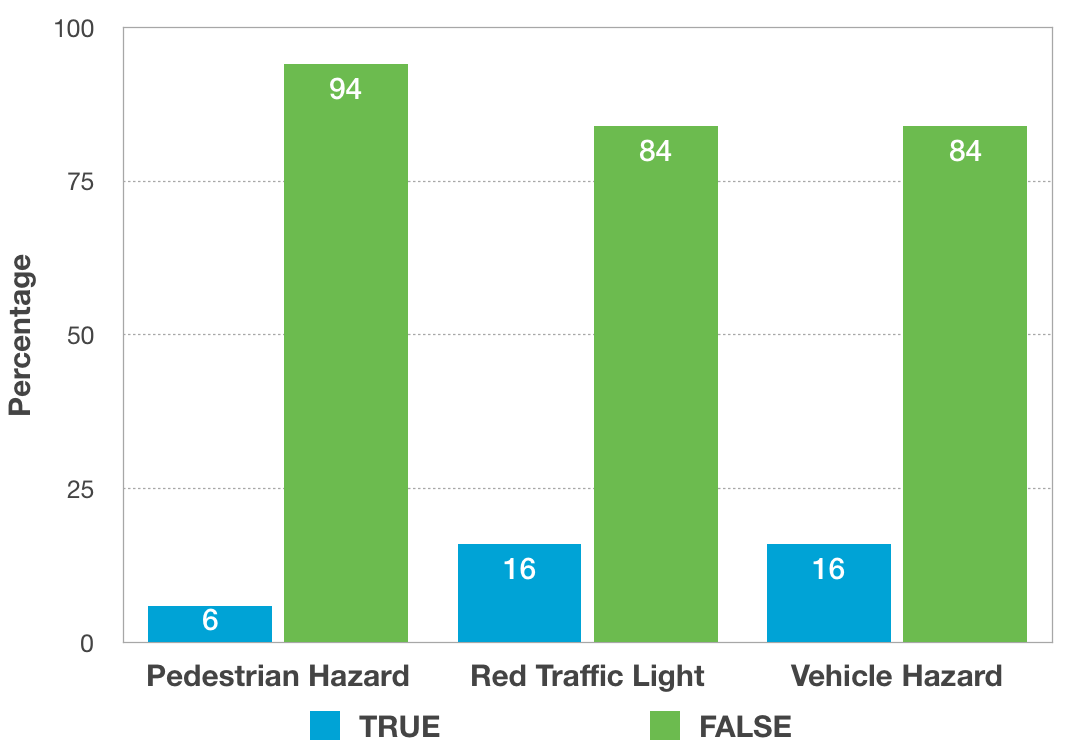
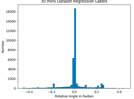
Figure 1: The distributions of affordances on the $\sim 30$ minutes training dataset.

In Figure 1, we show the distributions of the 30 minutes annotated dataset, which was used for training the affordances prediction network $g_{\phi}$. This dataset is a subset of the full 50 hours dataset, carefully sampled to maintain the same distribution as the full dataset.

3 Network Architectures

In Figure 2, we detail the architecture of our encoder, $h_{\phi}$. We follow the architecture presented in [Codevilla:2019] using the high level command, $c_{t}$, the image input, $I_{t}$ , and the speed variable $v_{t}$, as part of $o_{t}$. In Table 1, we detail the parameters of network architectures for different action-based representation learning approaches. We also detail the affordance projection network.

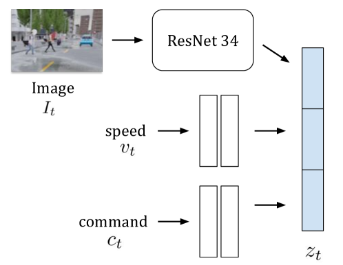
Figure 2: The architecture of the encoder $h_{\theta}$. Blue rectangles indicate that the features are appended. White rectangles are fully connected layers.

Input Output Num. of Module Dimension Channels Dropout ResNet 34 200 $\times$ 88 $\times$ 3 512 0.0 Speed 1 128 0.0 128 128 0.0 Command 4 128 0.0 128 128 0.0 Join 512+128+128 512 0.0 512 256 0.0 Action Branch 256 256 0.5 256 3 0.0 512 256 0.0 Speed Branch 256 256 0.5 256 1 0.0	Input Output Num. of Module Dimension Channels Dropout ResNet 34 200 $\times$ 88 $\times$ 3 512 0.0 Speed 1 128 0.0 128 128 0.0 Command 4 128 0.0 128 128 0.0 Join 512+128+128 512 0.0 Join ($Z_{t}$,$Z_{t+1}$) 512 + 512 512 0.0 512 256 0.0 Action ($a_{t}$) 256 256 0.0 256 3 0.0
(a) Behavior Cloning (BC)	(b) Inverse model
Input Output Num. of Module Dimension Channels Dropout ResNet 34 200 $\times$ 88 $\times$ 3 512 0.0 Speed 1 128 0.0 128 128 0.0 Command 4 128 0.0 128 128 0.0 3 512 0.0 Action ($a_{t}$) 512 256 0.0 256 512 0.0 Join 512+128+128 512 0.0 Join ($Z_{t}$, $Z_{t+1}$) 512 + 512 512 0.0 512 256 0.0 Action ($a_{t}$) 256 256 0.5 256 3 0.0 Join ($Z_{t}$, Action) 512 + 512 512 0.0	Input Output Num. of Module Dimension Channels Dropout 512 512 0.0 Affordances 512 256 0.0 256 M 0.0 (M: Classification - 2; Regression - 1)
(c) Forward Model	(d) Affordances Network

Table 1: Network architecture details for the encoders $h_{\theta}$ (a,b and c) and the affordance projection network $g_{\phi}$ (d) when fine-tuned for driving.

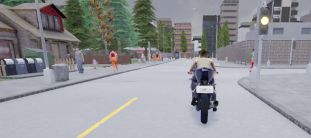
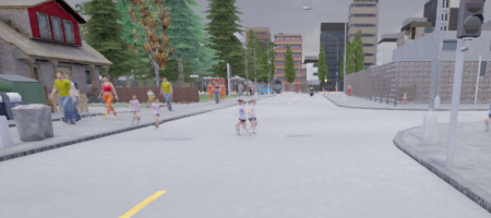
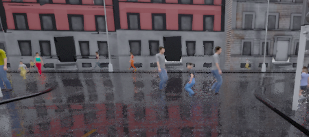
Figure 3: New types of vehicles and pedestrians present on the updated version of the benchmark. Left: motorbikes were not included on the previous benchmark. Middle: kids are now also part of pedestrians. Right: now pedestrians are able to better agglomerate when crossing roads.

4 Controller

To evaluate our models in the NoCrash benchmark, we tuned a controller using our affordances. Given a set of affordances at time $t$, $\{\psi(t),hv(t),hp(t),hr(t)\}$, the controller outputs an action $a(t)$ defined by $\{S(t),T(t),B(t)\}$, i.e., steering, throttle, and break, respectively. In particular, for lateral control (i.e., $S(t)$) and for longitudinal control (i.e., $T(t)$ and $B(t)$) we use the following PID-based equations:

$$S(t) =PID(\psi(t))=K_{p}\psi(t)+K_{i}\int_{0}^{t}\psi(\tau)d\tau+K_{d}\frac{\partial\psi(t)}{\partial t},$$

$$B(t) =max(hr(t),hp(t),hv(t)),$$

$$T(t) =PID(v\>\mbox{if}(B(t)>0),\>0\>\mbox{otherwise}),$$

where the hazard functions either equal to $1$ or $0$, and $v$ is the target maximum speed, 20Km/h in these experiments. We tuned the constants $K_{p},K_{i}$ and $K_{d}$ in town 1 (T1) to obtain a perfect driving (no errors, all episodes completed) for the dense condition of the NoCrash benchmark provided we use ground truth (perfect) affordances. We did it in that way to provide a driving evaluation directly depending on the quality of the affordance predictions, not in the controller itself, since it is not the focus of this paper.

5 Additional Results

Linear Probing. Tables 2 and 3 show the linear probing evaluation results of models tested on the $\sim 1$ hour Town01 testing set. This testing set has similar appearance to the training data. We observe a similar tendency to the results obtained on Town02, those shown in the main paper.

		Binary Affordances				Relative Angle ($\psi_{t}$)
Pre-training		Pedestrian ($hp$)	Vehicle ($hv$)	Red T.L. ($hr$)		Left Turn	Straight	Right Turn
No pre-training		$38\pm 1$	$59\pm 0$	$45\pm 0$		$10.03\pm 0.06$	$1.80\pm 0.03$	$17.57\pm 0.03$
ImageNet		$35\pm 1$	$67\pm 0$	$54\pm 1$		$14.46\pm 0.35$	$2.31\pm 0.09$	$19.06\pm 0.18$
Contrastive (ST-DIM)		$38\pm 0$	$57\pm 1$	$76\pm 1$		$6.72\pm 0.03$	$2.65\pm 0.03$	$13.12\pm 0.11$
Forward		$\underline{56\pm 0}$	$62\pm 0$	$55\pm 0$		$6.97\pm 0.12$	$\underline{\textbf{0.17}\pm 0.00}$	$5.88\pm 0.03$
Inverse		$\underline{\textbf{57}\pm 1}$	$\underline{82\pm 0}$	$\textbf{89}\pm 0$		$\underline{3.84\pm 0.06}$	$\underline{0.21\pm 0.03}$	$\textbf{2.96}\pm 0.09$
Behavior Cloning (BC)		$46\pm 0$	$\underline{\textbf{83}\pm 0}$	$86\pm 0$		$\underline{\textbf{3.76}\pm 0.03}$	$0.63\pm 0.00$	$4.35\pm 0.06$

Table 2: Linear probing results on Town01 testing set. Left: F1 score for the binary affordances (higher is better). Results are scaled by 100 for visualization purpose. Right: MAE of the relative angle (lower is better), shown for different navigation maneuvers. MAE is shown in degrees for an easier understanding.

		Binary Affordances				Relative Angle ($\psi_{t}$)
Pre-training		Pedestrian ($hp$)	Vehicle ($hv$)	Red T.L. ($hr$)		Left Turn	Straight	Right Turn
No pre-training		$38\pm 1$	$59\pm 0$	$45\pm 0$		$10.03\pm 0.06$	$1.80\pm 0.03$	$17.57\pm 0.03$
Contrastive (ST-DIM)		$36\pm 1$	$60\pm 2$	$67\pm 1$		$7.43\pm 0.17$	$2.79\pm 0.18$	$12.11\pm 0.18$
Contrastive Random (ST-DIM)		$34\pm 2$	$\textbf{78}\pm 1$	$52\pm 2$		$11.10\pm 0.52$	$2.02\pm 0.09$	$14.65\pm 0.29$
Forward		$\textbf{52}\pm 0$	$53\pm 0$	$60\pm 0$		$3.95\pm 0.00$	$0.11\pm 0.00$	$4.37\pm 0.03$
Forward Random		$5\pm 0$	$27\pm 0$	$2\pm 0$		$19.10\pm 0.03$	$0.63\pm 0.00$	$17.97\pm 0.03$
Inverse		$48\pm 1$	$71\pm 0$	$\textbf{90}\pm 0$		$\textbf{2.03}\pm 0.07$	$\textbf{0.21}\pm 0.03$	$\textbf{2.54}\pm 0.03$
Inverse Random		$34\pm 0$	$53\pm 0$	$55\pm 0$		$12.49\pm 0.45$	$0.84\pm 0.03$	$13.22\pm 0.54$

Table 3: Linear probing results on Town01 testing set, comparing encoders trained with random policy training data versus expert demonstration data. Note that, to provide fair comparison, the encoders here were trained with 20 hours data.

		Technique		Empty	Regular	Dense	T.L.
Training		BC driving		$72\pm 5$	$47\pm 2$	$20\pm 3$	$74\pm 2$
		BC pre-training		$\textbf{91}\pm 1$	$\textbf{91}\pm 4$	$\textbf{68}\pm 5$	$\textbf{8}\pm 1$
New Town		BC driving		$71\pm 2$	$42\pm 7$	$12\pm 3$	$63\pm 1$
		BC pre-training		$\textbf{83}\pm 3$	$\textbf{61}\pm 4$	$\textbf{25}\pm 4$	$\textbf{8}\pm 1$

Table 4: We compare the behavior cloning (BC) technique used as driving technique (BC driving) to it used as a pre-training technique (BC pre-training) for an affordances based model.

Driving Results. An important observation is that using expert demonstration as pre-training seems to be more beneficial than training a model end-to-end to directly perform control. In Table 4, we show a behavior cloning encoder trained with 50 hours of expert demonstrations. We compare two different uses of this encoder: directly producing driving controls and serving as representation learning for an affordance prediction model. With our pre-training strategy, and the complementary affordance training, our model (BC pre-training) is able to greatly outperform the end-to-end driving results (BC driving). This difference is expressive especially when comparing the capability to stop on red traffic lights. Finally, note that the “BC driving” results from Table 4 are in practice a re-training of the CILRS [Codevilla:2019] baseline to work on version 0.9.6.