EmoGraph: Capturing Emotion Correlations using Graph Networks
Abstract
Most emotion recognition methods tackle the emotion understanding task by considering individual emotion independently while ignoring their fuzziness nature and the interconnections among them. In this paper, we explore how emotion correlations can be captured and help different classification tasks. We propose EmoGraph that captures the dependencies among different emotions through graph networks. These graphs are constructed by leveraging the co-occurrence statistics among different emotion categories. Empirical results on two multi-label classification datasets demonstrate that EmoGraph outperforms strong baselines, especially for macro-F1. An additional experiment illustrates the captured emotion correlations can also benefit a single-label classification task.
1 Introduction
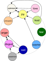
Understanding human emotions is considered as the key to building engaging dialogue systems Zhou et al. (2018). However, most works on emotion understanding tasks treat individual emotions independently while ignoring the fuzziness nature and the interconnections among them. A psychoevolutionary theory proposed by Plutchik (1984) shows that different emotions are actually correlated, and all emotions follow a circular structure. For example, “optimism” is close to “joy” and “anticipation” instead of “disgust” and “sadness”. Without considering the fundamental inter-correlation between them, the understanding of emotions can be unilateral, leading to sub-optimal performance. These understanding can be particularly important for low resource emotions, such as “surprise” and “trust” whose training samples are hard to get. Therefore, the research question we ask is, how can we obtain and incorporate the emotion correlation to improve emotion understanding tasks, such as classification?
To obtain emotion correlations, a possible way is to take advantage of a multi-label emotion dataset. Intuitively, emotions with high correlations will be labeled together, and therefore, emotion correlations can be extracted from the label co-occurrences. Recently, a multi-label emotion classification competition Mohammad et al. (2018) with 11 emotions has been introduced to promote research into emotional understanding. To tackle this challenge, the best team Baziotis et al. (2018) first pre-trains on a large amount of external emotion-related datasets and then performs transfer learning on this multi-label task. However, they still neglect the correlations between different emotions.
In this paper, we propose EmoGraph which leverages graph neural networks to model the dependencies between different emotions. We take each emotion as a node and first construct an emotion graph based on the co-occurrence statistics between every two emotion classes. Graph neural networks are then applied to extract the features from the neighbours of each emotion node. We conduct experiments on two multi-label emotion classification datasets. Empirical results show that our model outperforms strong baselines, especially for macro-F1 score. The analysis shows that low resource emotions, such as “trust”, can particularly benefit from the emotion correlations. An additional experiment illustrates that the captured emotion correlations can also help the single-label emotion classification task.
2 Related Work
For emotion classifications, Tang et al. (2016) proposed sentiment embeddings that incorporate sentiment information into word vectors. Felbo et al. (2017) trained a huge LSTM-based emotion representation by predicting emojis. Various methods have also been developed for automatic constructions of sentiment lexicons using both a supervised and unsupervised method Wang and Xia (2017). Duppada et al. (2018) combined both pretrained representations and emotion lexicon features, which significantly improved the emotion understanding systems. Park et al. (2018); Fung et al. ; Xu et al. (2018) encoded emotion information into word representations and demonstrated improvements over emotion classification tasks. Shin et al. (2019); Lin et al. (2019); Xu et al. (2019) further introduced emotion supervision into generation tasks.
Multi-label classification is an important yet challenging task in natural language processing. Binary relevance Boutell et al. (2004) transformed the multi-label problem into several independent classifiers. Other methods to model the dependencies have since been proposed by creating new labels Tsoumakas and Katakis (2007), using classifier chains Read et al. (2011), graphs Li et al. (2015), and RNN Chen et al. (2017); Yang et al. (2018). These models are either non-scalable or modeling the labels as a sequence.
Graph networks have been applied to model relations across different tasks such as image recognition Chen et al. (2019); Satorras and Estrach (2018), and text classification Ghosal et al. (2019); Yao et al. (2019) with different graph networks Kipf and Welling (2017); Veličković et al. (2018).
Despite the growing interests in low-resource studies in machine translation Artetxe et al. (2017); Lample et al. (2017), dialogue systems Bapna et al. (2017); Liu et al. (2019, 2020), speech recognition Miao et al. (2013); Thomas et al. (2013); Winata et al. (2020), emotion recognition Haider et al. (2020), and etc, emotion detection for low-resource emotions has been less studied.
3 Methodology
In this section, we first introduce the emotion graphs and then our emotion classification models. We denote the input sentence as and the emotion classes as . The label for is , where and denotes the label for . The embedding matrix is . The co-occurrence matrix of these emotions is .
3.1 Emotion Graphs
We take each emotion class as a node in the emotion graph. To create the connections between emotion nodes, we use the co-occurrence statistics between emotions. The intuition is that if two emotions co-occurs frequently, they will have a high correlation. Directly using this co-occurrence matrix as our graph may be problematic because the co-occurrence matrix is symmetric while the emotion relation is not symmetric. For example, in our corpus, “anticipation” co-occurs with “optimism” 197 times, while “anticipation” appears 425 times and “optimism” appears 1143 times. Thus, knowing “anticipation” and “optimism” co-occur is notably more important for “anticipation” than “optimism”. Thus, we calculate the co-occurrence matrix from a given emotion corpus and then normalize with so that the graph encodes the asymmetric relation between different emotions.
| (1) |
3.2 Emotion Classification Models
Our emotion classification model consists of an encoder and graph-based emotion classifiers following the framework of Chen et al. (2019). For the encoder, we choose the Transformer (TRS) Vaswani et al. (2017) and the pre-trained model BERT Devlin et al. (2019) for their strong representation capacities on many natural language tasks. We denote the encoded representation of as . For graph-based emotion classifiers, we experiment with two types of graph networks: GCN Kipf and Welling (2017) and GAT Veličković et al. (2018). The GCN takes the features of each emotion node as inputs and applies a convolution over neighboring nodes to generate the classifier for :
| (4) |
where is the normalized matrix of following Kipf and Welling (2017). is the embeddings for all emotions , and is the trainable parameters. Our emotion classifiers are , where is the classifier for . Alternatively, GAT takes the features of each node as input and learns a multi-head self-attention over the emotion nodes to generate classifiers .
We then simply take the inner product between and to compute , the logits of the emotion class for classification:
| (5) |
As our task is a multi-label prediction problem, we add a sigmoid activation to and use a cross-entropy loss function.
4 Experimental Setup
4.1 Dataset and Evaluation Metrics
We choose two datasets for our multi-label classification training and evaluation. SemEval-2018 Mohammad et al. (2018) contains 10,983 tweets with 11 different emotion categories. It is divided into three splits: training set (6838 samples), validation set (886 samples), and testing set (3259 samples). Due to its small label quantities and small dataset size, we crawled another Twitter dataset where we use emojis as emotion labels. We follow the same 64 emoji types as in Felbo et al. (2017) and collect 4 million twitter data, where each tweet has at least two emojis. We split them into 2.8 million (70%) for training, 0.4 million (10%) for validation and 0.8 million (20%) for testing.
Following the metrics in Mohammad et al. (2018), we use Jaccard accuracy, micro-average F1-score (micro-F1), and macro-average F1-score (macro-F1) as our evaluation metrics.
4.2 EmoGraph and Baselines
Our EmoGraph has four variants,TRS-GCN,TRS-GAT,BERT-GCN, and BERT-GAT, depending on the choice of sentence encoder (TRS/BERT) and graph networks (GCN/GAT). We compare our model to several strong baselines. NTUA-SLP Baziotis et al. (2018) is the top-1 system of the SemEval-2018 competition, which pre-trains the model on large amounts of external emotion-related datasets. DATN Yu et al. (2018) is the system that transfers sentiment information with dual attention transfer network. SGM Yang et al. (2018) models labels as a sequences and generates the labels using beam search. TRS is the system that adds a linear layer on top of the Transformer Vaswani et al. (2017). BERT is the system that adds a linear layer on top of the BERT Devlin et al. (2019).
| Accuracy | Micro-F1 | Macro-F1 | |
| NTUA-SLP | 58.8 | 70.1 | 52.8 |
| DATN | 58.3 | - | 54.4 |
| SGM | 48.2 | 57.5 | 41.1 |
| TRS | 51.1 | 63.4 | 46.7 |
| TRS-GAT | 51.7 | 64.6 | 48.3 |
| TRS-GCN | 51.9 | 63.8 | 49.2 |
| BERT | 58.4 | 70.1 | 53.8 |
| BERT-GAT | 58.3 | 69.9 | 56.9 |
| BERT-GCN | 58.9 | 70.7 | 56.3 |
| Accuracy | Micro-F1 | Macro-F1 | |
|---|---|---|---|
| TRS | 30.4 | 46.5 | 35.0 |
| SGM | 33.5 | 42.9 | 25.2 |
| TRS-GAT | 33.1 | 49.1 | 38.6 |
| TRS-GCN | 34.4 | 50.5 | 40.8 |
| F1 score | # Parameters | Anger | Fear | Happiness | Surprise | Sadness | Average F1 | Accuracy |
|---|---|---|---|---|---|---|---|---|
| LSTM | 1.11M | 72.7 | 12.2 | 53.7 | 31.3 | 69.3 | 46.2 | 66.7 |
| LSTM-GCN | 1.16M | 75.6 | 39.1 | 60.8 | 38.0 | 70.5 | 54.7 | 69.5 |
| BERT | 110M | 83.4 | 39.1 | 69.9 | 47.1 | 80.8 | 62.0 | 78.5 |
| BERT-GCN | 110M | 83.8 | 51.6 | 72.9 | 48.7 | 82.0 | 65.4 | 79.8 |
5 Results and Analysis
Results on two emotion classification datasets
The results on SemEval-2018 dataset are shown in Table 1, which illustrates several points. Firstly, BERT-GCN/TRS-GCN consistently improves over the baseline of BERT/TRS, in terms of accuracy (+0.5%/+0.8%), micro-F1 (+0.6%/+0.4%) and macro-F1 (+2.5%/+2.5%). It shows the effectiveness of the emotion graph by giving the performance boost on the strong baseline BERT, especially on the macro-F1 score. Secondly, our BERT-GCN achieves a 58.9% accuracy score, 70.7% micro-F1 score, and 56.3% macro-F1 score, which beats the best system NTUA-SLP in terms of all metrics, without using any affect features or pre-training on emotional datasets. Thirdly, EmoGraph is particularly effective in macro-F1. For example, BERT-GAT is 2.5% better than DATN and 3.1% better than BERT.
We notice that for both accuracy and micro-F1, the improvements of graph networks are very marginal on the SemEval-2018 dataset. This is because the small emotion label space (only 11 emotions) limits the effectiveness of emotion graphs. Thus, we train our models on another Twitter dataset with 64 emoji labels. Table 2 shows both TRS-GCN and TRS-GAT consistently improves TRS with a large margin for all metrics, which shows that graph networks are better at dealing with rich emotion information.111Data statistics, training details, and ablation studies for threshold (Eq. 2) and weight (Eq. 3) are in the appendix.
| Surprise | Trust | |
|---|---|---|
| BERT | 18.7 | 6.9 |
| BERT-GAT | 31.9 | 14.8 |
| BERT-GCN | 27.8 | 24.3 |
Connection to the wheel of emotions
Following the positioning of the wheel of emotion Plutchik (1984), we visualize the graph structure in Figure 1. It shows that our emotion graph can be divided into three sub-graphs, 1) the nodes connected with “disgust”, 2) “fear” 3) the nodes connected with “joy”. Most nodes are locally connected, which means the positioning in the wheel of emotion does contain the correlation information. One exception is that “anticipation” is also close to “anger” in the wheel of emotions, which is not true in our case. Another exception we found is that “surprise” is close to “joy” in our emotion graph while they are quite far away from each other in the wheel of emotions. We believe it reflects the bias when people post tweets online, and the distance between neighboring emotions are not quantitatively the same as the wheel of emotions.
Analysis on low resource emotions
Table 4 shows that the significant improvements in terms of the macro-F1 on the SemEval-2018 dataset mainly come from the low resource emotions, such as “surprise” and “trust”, where only 5% of the labels are positive. From Figure 1, we observe that both “surprise” and “trust” are connected to “joy”, which has 39.3% samples labeled as positive. We conjecture that low resource emotion classifiers learn effective inductive bias through connections with high-resource emotion classes, such as “joy” and “optimism”, and achieve better performances.
Generalization to single emotion classification task
To verify the generalization ability of EmoGraph, we conduct an extra experiment on IEMOCAP dataset Busso et al. (2008), which is a single label multi-class classification dataset. We only use the six emotions that overlap with the SemEval-2018 task, which are “anger”, “sadness”, “happiness”, “disgust”, “fear” and “surprise” with 2931 samples (the graph matrix G is obtained from the SemEval-2018 dataset). We then train our EmoGraph using either a one-layer LSTM with attention or BERT as an encoder and GCN as the graph structure. To adapt the change from 11 emotions to 6 emotions, we only train the classifiers corresponding to those six emotions. The results with 10-fold cross-validation are reported in Table 3. We didn’t report “disgust” as there are less than five positive examples. The results confirm that with captured emotion correlations, classification performances can be improved by 2.8%/8.5% accuracy/average F1 score using LSTM encoder and 1.3%/3.4% accuracy/average F1 score using BERT encoder. Surprisingly, for both encoders with GCN improves more than 10% on “fear” (a low-resource emotion in the IEMOCAP dataset), although it doesn’t have connections with other emotions in the graph. We conjecture that the improvements come from the shared representation of in Eq. 4 among all emotion categories, which helps our model optimize to a better local minimal.
6 Conclusion
In this paper, we proposed EmoGraph which leverages graph neural networks to model the dependencies among different emotions. We consider each emotion as a node and construct an emotion graph based on the co-occurrence statistics. Our model with EmoGraph outperforms the existing strong multi-label classification baselines. Our analysis shows EmoGraph is especially helpful for low resource emotions and large emotion space. An additional experiment shows that it can also help a single-label emotion classification task.
Acknowledgments
This work is partially funded by ITF/319/16FP, HKUST 16248016 of Hong Kong Research Grants Council and MRP/055/18 of the Innovation Technology Commission, the Hong Kong SAR Government.
References
- Artetxe et al. (2017) Mikel Artetxe, Gorka Labaka, Eneko Agirre, and Kyunghyun Cho. 2017. Unsupervised neural machine translation. arXiv preprint arXiv:1710.11041.
- Bapna et al. (2017) Ankur Bapna, Gokhan Tür, Dilek Hakkani-Tür, and Larry Heck. 2017. Towards zero-shot frame semantic parsing for domain scaling. Proc. Interspeech 2017, pages 2476–2480.
- Baziotis et al. (2018) Christos Baziotis, Athanasiou Nikolaos, Alexandra Chronopoulou, Athanasia Kolovou, Georgios Paraskevopoulos, Nikolaos Ellinas, Shrikanth Narayanan, and Alexandros Potamianos. 2018. Ntua-slp at semeval-2018 task 1: Predicting affective content in tweets with deep attentive rnns and transfer learning. In Proceedings of The 12th International Workshop on Semantic Evaluation, pages 245–255.
- Boutell et al. (2004) Matthew R Boutell, Jiebo Luo, Xipeng Shen, and Christopher M Brown. 2004. Learning multi-label scene classification. Pattern recognition, 37(9):1757–1771.
- Busso et al. (2008) Carlos Busso, Murtaza Bulut, Chi-Chun Lee, Abe Kazemzadeh, Emily Mower, Samuel Kim, Jeannette N Chang, Sungbok Lee, and Shrikanth S Narayanan. 2008. Iemocap: Interactive emotional dyadic motion capture database. Language resources and evaluation, 42(4):335.
- Chen et al. (2017) Guibin Chen, Deheng Ye, Zhenchang Xing, Jieshan Chen, and Erik Cambria. 2017. Ensemble application of convolutional and recurrent neural networks for multi-label text categorization. In 2017 International Joint Conference on Neural Networks (IJCNN), pages 2377–2383. IEEE.
- Chen et al. (2019) Zhao-Min Chen, Xiu-Shen Wei, Peng Wang, and Yanwen Guo. 2019. Multi-label image recognition with graph convolutional networks. In Proceedings of the IEEE Conference on Computer Vision and Pattern Recognition, pages 5177–5186.
- Devlin et al. (2019) Jacob Devlin, Ming-Wei Chang, Kenton Lee, and Kristina Toutanova. 2019. Bert: Pre-training of deep bidirectional transformers for language understanding. In Proceedings of the 2019 Conference of the North American Chapter of the Association for Computational Linguistics: Human Language Technologies, Volume 1 (Long and Short Papers), pages 4171–4186.
- Duppada et al. (2018) Venkatesh Duppada, Royal Jain, and Sushant Hiray. 2018. Seernet at semeval-2018 task 1: Domain adaptation for affect in tweets. In Proceedings of The 12th International Workshop on Semantic Evaluation, pages 18–23.
- Felbo et al. (2017) Bjarke Felbo, Alan Mislove, Anders Søgaard, Iyad Rahwan, and Sune Lehmann. 2017. Using millions of emoji occurrences to learn any-domain representations for detecting sentiment, emotion and sarcasm. In Proceedings of the 2017 Conference on Empirical Methods in Natural Language Processing, pages 1615–1625.
- (11) Pascale Fung, Dario Bertero, Peng Xu, Ji Ho Park, Chien-Sheng Wu, and Andrea Madotto. Empathetic dialog systems.
- Ghosal et al. (2019) Deepanway Ghosal, Navonil Majumder, Soujanya Poria, Niyati Chhaya, and Alexander Gelbukh. 2019. Dialoguegcn: A graph convolutional neural network for emotion recognition in conversation. In Proceedings of the 2019 Conference on Empirical Methods in Natural Language Processing and the 9th International Joint Conference on Natural Language Processing (EMNLP-IJCNLP), pages 154–164.
- Haider et al. (2020) Fasih Haider, Senja Pollak, Pierre Albert, and Saturnino Luz. 2020. Emotion recognition in low-resource settings: An evaluation of automatic feature selection methods. Computer Speech & Language, page 101119.
- Kipf and Welling (2017) Thomas N Kipf and Max Welling. 2017. Semi-supervised classification with graph convolutional networks. In International Conference on Learning Representations.
- Lample et al. (2017) Guillaume Lample, Alexis Conneau, Ludovic Denoyer, and Marc’Aurelio Ranzato. 2017. Unsupervised machine translation using monolingual corpora only. arXiv preprint arXiv:1711.00043.
- Li et al. (2018) Qimai Li, Zhichao Han, and Xiao-Ming Wu. 2018. Deeper insights into graph convolutional networks for semi-supervised learning. In Thirty-Second AAAI Conference on Artificial Intelligence.
- Li et al. (2015) Shoushan Li, Lei Huang, Rong Wang, and Guodong Zhou. 2015. Sentence-level emotion classification with label and context dependence. In Proceedings of the 53rd Annual Meeting of the Association for Computational Linguistics and the 7th International Joint Conference on Natural Language Processing (Volume 1: Long Papers), pages 1045–1053.
- Lin et al. (2019) Zhaojiang Lin, Andrea Madotto, Jamin Shin, Peng Xu, and Pascale Fung. 2019. Moel: Mixture of empathetic listeners. In Proceedings of the 2019 Conference on Empirical Methods in Natural Language Processing and the 9th International Joint Conference on Natural Language Processing (EMNLP-IJCNLP), pages 121–132.
- Liu et al. (2019) Zihan Liu, Jamin Shin, Yan Xu, Genta Indra Winata, Peng Xu, Andrea Madotto, and Pascale Fung. 2019. Zero-shot cross-lingual dialogue systems with transferable latent variables. In Proceedings of the 2019 Conference on Empirical Methods in Natural Language Processing and the 9th International Joint Conference on Natural Language Processing (EMNLP-IJCNLP), pages 1297–1303.
- Liu et al. (2020) Zihan Liu, Genta Indra Winata, Peng Xu, and Pascale Fung. 2020. Coach: A coarse-to-fine approach for cross-domain slot filling. In Proceedings of the 58th Annual Meeting of the Association for Computational Linguistics, pages 19–25, Online. Association for Computational Linguistics.
- Miao et al. (2013) Yajie Miao, Florian Metze, and Shourabh Rawat. 2013. Deep maxout networks for low-resource speech recognition. In 2013 IEEE Workshop on Automatic Speech Recognition and Understanding, pages 398–403. IEEE.
- Mohammad et al. (2018) Saif Mohammad, Felipe Bravo-Marquez, Mohammad Salameh, and Svetlana Kiritchenko. 2018. Semeval-2018 task 1: Affect in tweets. In Proceedings of The 12th International Workshop on Semantic Evaluation, pages 1–17.
- Park et al. (2018) Ji Ho Park, Peng Xu, and Pascale Fung. 2018. Plusemo2vec at semeval-2018 task 1: Exploiting emotion knowledge from emoji and# hashtags. In Proceedings of The 12th International Workshop on Semantic Evaluation, pages 264–272.
- Plutchik (1984) Robert Plutchik. 1984. Emotions: A general psychoevolutionary theory. Approaches to emotion, 1984:197–219.
- Read et al. (2011) Jesse Read, Bernhard Pfahringer, Geoff Holmes, and Eibe Frank. 2011. Classifier chains for multi-label classification. Machine learning, 85(3):333.
- Satorras and Estrach (2018) Victor Garcia Satorras and Joan Bruna Estrach. 2018. Few-shot learning with graph neural networks. In International Conference on Learning Representations.
- Shin et al. (2019) Jamin Shin, Peng Xu, Andrea Madotto, and Pascale Fung. 2019. Happybot: Generating empathetic dialogue responses by improving user experience look-ahead. arXiv preprint arXiv:1906.08487.
- Tang et al. (2016) Duyu Tang, Furu Wei, Bing Qin, Nan Yang, Ting Liu, and Ming Zhou. 2016. Sentiment embeddings with applications to sentiment analysis. IEEE Transactions on Knowledge and Data Engineering, 28(2):496–509.
- Thomas et al. (2013) Samuel Thomas, Michael L Seltzer, Kenneth Church, and Hynek Hermansky. 2013. Deep neural network features and semi-supervised training for low resource speech recognition. In 2013 IEEE international conference on acoustics, speech and signal processing, pages 6704–6708. IEEE.
- Tsoumakas and Katakis (2007) Grigorios Tsoumakas and Ioannis Katakis. 2007. Multi-label classification: An overview. International Journal of Data Warehousing and Mining (IJDWM), 3(3):1–13.
- Vaswani et al. (2017) Ashish Vaswani, Noam Shazeer, Niki Parmar, Jakob Uszkoreit, Llion Jones, Aidan N Gomez, Łukasz Kaiser, and Illia Polosukhin. 2017. Attention is all you need. In Advances in neural information processing systems, pages 5998–6008.
- Veličković et al. (2018) Petar Veličković, Guillem Cucurull, Arantxa Casanova, Adriana Romero, Pietro Liò, and Yoshua Bengio. 2018. Graph attention networks. In International Conference on Learning Representations.
- Wang and Xia (2017) Leyi Wang and Rui Xia. 2017. Sentiment lexicon construction with representation learning based on hierarchical sentiment supervision. In Proceedings of the 2017 Conference on Empirical Methods in Natural Language Processing, pages 502–510.
- Winata et al. (2020) Genta Indra Winata, Samuel Cahyawijaya, Zihan Liu, Zhaojiang Lin, Andrea Madotto, Peng Xu, and Pascale Fung. 2020. Learning fast adaptation on cross-accented speech recognition. arXiv preprint arXiv:2003.01901.
- Xu et al. (2018) Peng Xu, Andrea Madotto, Chien-Sheng Wu, Ji Ho Park, and Pascale Fung. 2018. Emo2vec: Learning generalized emotion representation by multi-task training. In Proceedings of the 9th Workshop on Computational Approaches to Subjectivity, Sentiment and Social Media Analysis, pages 292–298.
- Xu et al. (2019) Peng Xu, Chien-Sheng Wu, Andrea Madotto, and Pascale Fung. 2019. Clickbait? sensational headline generation with auto-tuned reinforcement learning. In Proceedings of the 2019 Conference on Empirical Methods in Natural Language Processing and the 9th International Joint Conference on Natural Language Processing (EMNLP-IJCNLP), pages 3056–3066.
- Yang et al. (2018) Pengcheng Yang, Xu Sun, Wei Li, Shuming Ma, Wei Wu, and Houfeng Wang. 2018. Sgm: Sequence generation model for multi-label classification. In Proceedings of the 27th International Conference on Computational Linguistics, pages 3915–3926.
- Yao et al. (2019) Liang Yao, Chengsheng Mao, and Yuan Luo. 2019. Graph convolutional networks for text classification. In Proceedings of the AAAI Conference on Artificial Intelligence, volume 33, pages 7370–7377.
- Yu et al. (2018) Jianfei Yu, Luís Marujo, Jing Jiang, Pradeep Karuturi, and William Brendel. 2018. Improving multi-label emotion classification via sentiment classification with dual attention transfer network. In Proceedings of the 2018 Conference on Empirical Methods in Natural Language Processing, pages 1097–1102, Brussels, Belgium. Association for Computational Linguistics.
- Zhou et al. (2018) Li Zhou, Jianfeng Gao, Di Li, and Heung-Yeung Shum. 2018. The design and implementation of xiaoice, an empathetic social chatbot. arXiv preprint arXiv:1812.08989.
Appendix A Appendices
A.1 Preprocessing
To cope with the noise in the twitter data, we lowercase the tweets, remove the “#” punctuation and replace “URL link” with a special token <url>, “user mentions” with <user> and “number” with <num>. For example, one original tweet ”@JessicaZ00 @ZRlondon ditto!! Such an amazing atmosphere! We have 10 people here. #LondonEvents #cheer” will be cleaned as ”<user> <user> ditto! such an amazing atmosphere! we have <num> people here. londonevents cheer”. By doing so, we can reduce the vocabulary size and make the model easier to learn.
A.2 Training Details
To train the SemEval-2018, we calculate the co-occurrence matrix based on the training and development sets. We set the threshold as 0.4, and the weight as 0.35 for GCN. We set the threshold as 0.5 for GAT. For both BERT-GCN and BERT-GAT, the emotion label embeddings are initialized with 300-dim GloVe vectors. For the BERT structure, we choose 12 layers BERT-base model, and the hidden size of the graph is set to 768. An Adam optimizer with the learning rate 1e-4 is used to train the graph networks. Another Adam optimizer is used to train the BERT model with the learning set as 2e-5 and dropout rate as 0.3. For TRS-GCN and TRS-GAT, the hidden size of the graph network is set to 200. The heads of the Transformer are 4, and the depth is 44. An Adam optimizer is used to train the full model with a 0.001 learning rate. For the Twitter dataset, we calculate the co-occurrence matrix based on the training set. We set the threshold as 0.1, and the weight is set as 0.35 for both. We use the TRS as the sentence encoder. The hidden size of both graph networks and TRS are 200. The heads of TRS are 6, and the depth is 120. An Adam optimizer is used to train our model with a 0.001 learning rate.
To train IEMOCAP dataset, the parameters of both GCN and BERT follow the same setting as in SemEval 2018 task. For the LSTM based method, we set the hidden size of LSTM encoder as 200 and initialize the word embedding with GloVe. An Adam optimizer with a learning rate of 0.001 is used to optimize all parameters.
| Anger | Anticipation | Disgust | Fear | Joy | Love |
|---|---|---|---|---|---|
| 36.1 | 13.9 | 36.6 | 16.8 | 39.3 | 12.3 |
| Optimism | Pessimism | Sadness | Surprise | Trust | |
| 31.3 | 11.6 | 29.4 | 5.2 | 5.0 |
| 33.37 | 21.86 | 38.13 | 16.63 | 0.41 | 15.40 | 3.71 | 4.35 |
| 32.95 | 0.95 | 3.78 | 1.43 | 5.02 | 0.21 | 3.13 | 10.13 |
| 2.59 | 0.26 | 9.67 | 4.40 | 2.18 | 2.83 | 4.86 | 2.23 |
| 1.39 | 1.58 | 3.50 | 3.03 | 1.98 | 3.35 | 1.14 | 3.73 |
| 2.92 | 3.21 | 9.91 | 0.51 | 2.16 | 4.00 | 3.30 | 2.97 |
| 5.14 | 3.66 | 1.69 | 1.89 | 2.43 | 6.95 | 2.10 | 2.56 |
| 0.19 | 3.83 | 1.35 | 3.49 | 1.55 | 2.12 | 2.83 | 0.78 |
| 1.48 | 2.03 | 0.94 | 0.25 | 1.28 | 0.53 | 0.56 | 0.28 |
| F1 score | Anger | Fear | Happiness | Surprise | Sadness |
| Distribution(%) | 37.7 | 1.4 | 20.1 | 3.5 | 37.2 |
A.3 Data Statistics
The data statistics for the SemEval-2018, Twitter and IEMOCAP are shown in Table 5, Table 6, and Table 7, respectively.
From Table 5, we can see that in the SemEval-2018 dataset, only 5.2% and 5.0% samples are labeled as positive for “surprise” and “trust”, respectively. And from Table 7, we can see that in the IEMOCAP dataset, only 1.4% samples are labeled as positive for “fear”.
A.4 Effects of threshold and weight
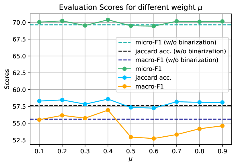
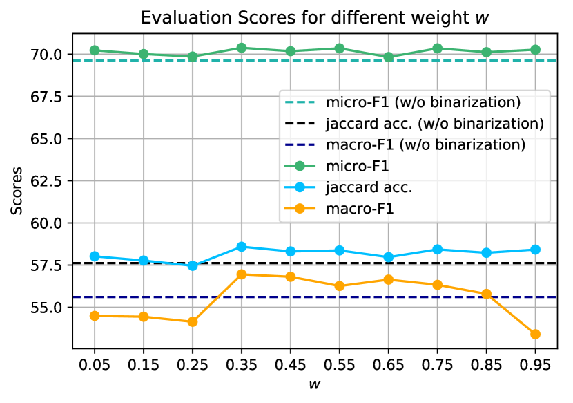
As illustrated in Figure 3 and Figure 3, we plot the diagram of accuracy, micro-F1 and macro-F1 on the test set by varying and , respectively, for BERT-GCN. We also include another baseline BERT-GCN model which is trained by setting (w/o binarization), to see the effects of binarization (Eq. 2) and weighting (Eq. 3).
Figure 3 shows that removing moderate amount of noisy connections by changing can improve the performance. For macro-F1, it clearly shows that small achieves much better results than large . If is large, useful emotion connections might be cut off, therefore leading to worse results.
Figure 3 shows that for accuracy and micro-F1, changing can achieve better performance than the baseline without binarization and weighting.