Flux-mortar mixed finite element methods on non-matching grids

Abstract

We investigate a mortar technique for mixed finite element approximations of Darcy flow on non-matching grids in which the normal flux is chosen as the coupling variable. It plays the role of a Lagrange multiplier to impose weakly continuity of pressure. In the mixed formulation of the problem, the normal flux is an essential boundary condition and it is incorporated with the use of suitable extension operators. Two such extension operators are considered and we analyze the resulting formulations with respect to stability and convergence. We further generalize the theoretical results, showing that the same domain decomposition technique is applicable to a class of saddle point problems satisfying mild assumptions. An example of coupled Stokes-Darcy flows is presented.

65N12, 65N15, 65N55

1 Introduction

The mortar mixed finite element method [3, 4] has proven to be an efficient and flexible domain decomposition technique for solving a wide range of single-physics or multiphysics problems described by partial differential equations in mixed formulations coupled through interfaces with non-matching grids. The key attribute of this method is the introduction of a Lagrange multiplier, referred to as the mortar variable, on the interface that enforces continuity of the solution. The method can be implemented as an iterative algorithm that requires only subdomain solves on each iteration.

We consider porous media flow in a mixed formulation as our leading example. In this context, the two most natural choices for the mortar variable are the pressure or the normal Darcy flux. In the case of matching grids, domain decomposition methods with these two types of Lagrange multipliers were introduced in [19]. In [3], a mortar mixed finite element method on non-matching grids with a pressure mortar was developed. A multiscale version of the method, referred to as the multiscale mortar mixed finite element method (MMMFEM), was developed in [4]. In this case pressure continuity is enforced by construction and normal flux continuity is enforced in a weak sense. This strategy has been successfully applied to more general applications as well, including coupled single-phase and multiphase flows in porous media [29], nonlinear elliptic problems [5], coupled Stokes and Darcy flows [18, 24, 15], and mixed formulations of linear elasticity [21].

In this work, we explore the mortar mixed finite element method in which the normal flux across each interface acts as the mortar variable. In this case, normal flux continuity is imposed by construction and continuity of pressure is imposed weakly. Our specific interest lies in deriving a priori error estimates in the presence of non-matching grids. To the best of our knowledge, such analysis has not been previously done.

A challenge that arises in this approach is that the normal flux is an essential boundary condition for mixed Darcy formulations and needs to be incorporated accordingly. We achieve this by introducing appropriate extension operators in the definitions of the velocity spaces in both the continuous and the discrete settings. This involves solving Neumann problems for each subdomain. We employ a Lagrange multiplier to remedy both the potential incompatibility of the data as well as the uniqueness of the solution.

Let us highlight the four main contributions presented in this work. First, our focus is on non-matching grids and we quantify the role this non-conformity plays in the context of a priori error analysis. Two projection operators are proposed that require separate analyses and lead to slightly different error estimates. Second, we consider a reduction of the problem to a symmetric, positive definite system that contains only the mortar variable. An iterative scheme is then proposed to solve this reduced system such that the solution conserves mass locally at each iteration. Third, the theoretical framework is presented in a general setting that is applicable to a broad class of saddle point problems. Fourth, we explicitly consider an important example, namely coupled Stokes-Darcy problems, [24, 11, 15, 18]. A key component is developing a flux-mortar finite element method for Stokes. Previously, only normal stress mortar methods for Stokes have been considered, with the mortar variable being used to impose weakly continuity of the velocity [6, 18, 22]. While a velocity Lagrange multiplier has been employed in domain decomposition methods for Stokes with matching grids [27, 25], to the best of our knowledge this is the first Stokes discretization on non-matching grids with velocity mortar variable. Moreover, we develop a new parallel domain decomposition method for the Stokes-Darcy problem, which satisfies velocity or flux continuity at each iteration. We refer the reader to [12, 35, 16] for some of the previous works on domain decomposition methods for coupled Stokes and Darcy flows. In these works, flux continuity is either relaxed via the use of Robin transmission conditions [12] or it is satisfied only at convergence using pressure and normal stress mortars [35, 16].

For the sake of clarity of the presentation, we focus on the case of subdomain and mortar grids being on the same scale. However, the flux-mortar mixed finite element method can be formulated as a multiscale method via the use of coarse scale mortar grids, as was done in [4]. In this case, following the approach in [17], the method can be implemented using an interface multiscale pressure basis, which can be computed by solving local subdomain problems with specified mortar flux boundary data.

We note several similarities and relationships between the flux-mortar method and existing schemes. First, as mentioned, our approach is dual to the pressure mortar technique that is central to the MMMFEM [3, 4]. Second, the multiscale hybrid-mixed (MHM) method [20, 1] similarly introduces flux degrees of freedom on the interfaces between elements to impose weakly continuity of pressure. The difference is that the MHM is defined on a single global grid and it is based on an elliptic formulation, rather than a mixed formulation. The MHM is related to a special case of the mixed subgrid upscaling method proposed in [2]. The latter does not involve a Lagrange multiplier, but incorporates global flux continuity via a coarse scale mixed finite element velocity space, which may include additional degrees of freedom internal to the subdomains. In contrast, our method reduces to an interface problem involving only mortar degrees of freedom. Furthermore, the analysis in [2] does not allow for non-matching grids along the coarse scale interfaces. Finally, we note that the flux-mortar mixed finite element method has been successfully applied in the context of fracture flow [9, 26] and coupled Stokes-Darcy flow [8]. The analysis in [9] exploits that there is tangential flow along the fractures and does not cover the domain decomposition framework considered in this work, while the analysis in [8] focuses on robust preconditioning.

The article is structured as follows. Section 2 introduces the model problem and its domain decomposition formulation. The mixed finite element discretization is introduced in Section 3 and we present two projection operators to handle the non-matching grids. The well posedness of the method is established in Section 4. Section 5 provides a priori error estimates for the proposed discretization. The problem is then reduced to an interface formulation that involves only the mortar variables in Section 6. We generalize these concepts and results to a more abstract setting in Section 7 and show how to apply them to a general class of saddle point problems. The general framework is applied to the Stokes-Darcy problem. Finally, we verify the a priori error analysis with numerical experiments in Section 8.

2 The model problem

We introduce the flux-mortar method using an accessible model problem given by the mixed formulation of the Poisson problem. Let $\Omega\subset\mathbb{R}^{n}$, $n=2,3$ be a bounded polygonal domain. The model problem is

(2.1) $$\bm{u}=-K\nabla p,\quad\nabla\cdot\bm{u}=f\ \mbox{ in }\Omega,\quad p=0\ \mbox{ on }\partial\Omega.$$

We will use the terminology common to porous media flow modeling. Hence, we refer to $\bm{u}$ as the Darcy velocity, $p$ is the pressure, $K$ is a uniformly bounded symmetric positive-definite conductivity tensor, and $f\in L^{2}(\Omega)$ is a source function. We assume that there exist $0<k_{min}<k_{max}<\infty$ such that $\forall\bm{x}\in\Omega$,

(2.2) $$k_{min}\xi^{T}\xi\leq\xi^{T}K(\bm{x})\xi\leq k_{max}\xi^{T}\xi,\quad\forall\xi\in\mathbb{R}^{n}.$$

We will use the following standard notation. For $G$ a domain in $\mathbb{R}^{n}$, $n=2,3$, or a manifold in $\mathbb{R}^{n-1}$, the Sobolev spaces on $G$ are denoted by $W^{k,p}(G)$. Let $H^{k}(G):=W^{k,2}(G)$ and $L^{2}(G):=H^{0}(G)$. The $L^{2}(G)$-inner product or duality pairing is denoted by $(\cdot,\cdot)_{G}$. For $G\subset\mathbb{R}^{n}$, let

$$H(\operatorname{div},G)=\{\bm{v}\in(L^{2}(G))^{n}:\nabla\cdot\bm{v}\in L^{2}(G)\}.$$

We use the following shorthand notation to denote the norms of these spaces:

$$\|f\|_{k,G} :=\|f\|_{H^{k}(G)}, \|f\|_{G} :=\|f\|_{0,G}, \|\bm{v}\|_{\operatorname{div},G}^{2} :=\|\bm{v}\|_{H(\operatorname{div},G)}^{2}=\|\bm{v}\|_{G}^{2}+\|\nabla\cdot\bm{v}\|_{G}^{2}.$$

We use the binary relation $a\lesssim b$ to imply that a constant $C>0$ exists, independent of the mesh size $h$, such that $a\leq Cb$. The relationship $\gtrsim$ is defined analogously.

The variational formulation of (2.1) is: Find $(\bm{u},p)\in H(\operatorname{div},\Omega)\times L^{2}(\Omega)$ such that

(2.3a) $$(K^{-1}\bm{u},\bm{v})_{\Omega}-(p,\nabla\cdot\bm{v})_{\Omega} =0, \forall\bm{v} \in H(\operatorname{div},\Omega),$$

(2.3b) $$(\nabla\cdot\bm{u},w)_{\Omega} =(f,w)_{\Omega}, \forall w \in L^{2}(\Omega).$$

It is well known that (2.3) has a unique solution [7].

2.1 Domain decomposition

The domain $\Omega$ is decomposed into disjoint polygonal subdomains $\Omega_{i}$ with $i\in I_{\Omega}=\{1,2,\ldots,n_{\Omega}\}$. Let $\bm{\nu}_{i}$ denote the outward unit vector normal to the boundary $\partial\Omega_{i}$. The $(n-1)$-dimensional interface between two subdomains $\Omega_{i}$ and $\Omega_{j}$ is denoted by $\Gamma_{ij}:=\partial\Omega_{i}\cap\partial\Omega_{j}$. Each interface $\Gamma_{ij}$ is assumed to be Lipschitz and endowed with a unique, unit normal vector $\bm{\nu}$ such that $\bm{\nu}:=\bm{\nu}_{i}=-\bm{\nu}_{j}\text{ on }\Gamma_{ij},\ i<j.$ Let $\Gamma:=\bigcup_{i<j}\Gamma_{ij}$ and $\Gamma_{i}:=\Gamma\cap\partial\Omega_{i}$. We categorize $\Omega_{i}$ as an interior subdomain if $\partial\Omega_{i}\subseteq\Gamma$, i.e. if none of its boundaries coincide with the boundary of the domain $\Omega$. Let $I_{int}:=\{i\in I_{\Omega}:\ \partial\Omega_{i}\subseteq\Gamma\}$. For given $\Omega_{i}$, let the local velocity and pressure function spaces $V_{i}$ and $W_{i}$, respectively, be defined as

$$V_{i}:=H(\operatorname{div},\Omega_{i}),\quad W_{i}:=L^{2}(\Omega_{i}).$$

Let the composite function spaces be defined as

$$V:=\bigoplus_{i}V_{i},\quad W:=\bigoplus_{i}W_{i}=L^{2}(\Omega).$$

Let

$$V_{i}^{0}:=\{\bm{v}_{h,i}\in V_{i}:\ (\bm{\nu}_{i}\cdot\bm{v})|_{\Gamma_{i}}=0\},\quad V^{0}:=\bigoplus_{i}V_{i}^{0}.$$

The normal flux $\bm{\nu}\cdot\bm{u}$ on $\Gamma$ will be modeled by a Lagrange multiplier $\lambda\in\Lambda$, with

$$\Lambda :=L^{2}(\Gamma).$$

We note that $\Lambda$ has more regularity than the normal trace of $V_{i}$. For $\lambda\in\Lambda$, we use a subscript to indicate its relative orientation with respect to the adjacent subdomains:

$$\lambda_{i}:=\lambda,\ \ \lambda_{j}:=-\lambda\ \ \text{ on }\Gamma_{ij},\ i<j.$$

In particular, $\lambda_{i}$ models $\bm{\nu}_{i}\cdot\bm{u}$ and $\lambda_{j}$ models $\bm{\nu}_{j}\cdot\bm{u}$ on $\Gamma_{ij}$.

Next, we associate appropriate norms to the function spaces. The spaces $W$ and $\Lambda$ are equipped with the standard $L^{2}(\Omega)$ and $L^{2}(\Gamma)$ norms, respectively. The space $V$, which does not have any continuity imposed on the interfaces, hence $V\not\subset H(\operatorname{div},\Omega)$, is equipped with a broken $H(\operatorname{div})$ norm. Letting $\bm{v}_{i}=\bm{v}|_{\Omega_{i}}$, we define

$$\|\bm{v}\|_{V} :=\sum_{i}\|\bm{v}_{i}\|_{\operatorname{div},\Omega_{i}}, \|w\|_{W} :=\|w\|_{\Omega}, \|\mu\|_{\Lambda} :=\|\mu\|_{\Gamma}.$$

3 Discretization

In this section we describe the flux-mortar mixed finite element method for (2.3). For subdomain $\Omega_{i}$, let $\Omega_{h,i}$ be a shape-regular tessellation with typical mesh size $h$ consisting of affine finite elements. The grids $\Omega_{h,i}$ and $\Omega_{h,j}$ may be non-matching along the interface $\Gamma_{ij}$. Let $V_{h,i}\times W_{h,i}\subset V_{i}\times W_{i}$ be a pair of conforming finite element spaces that is stable for the mixed formulation of the Poisson problem, i.e.,

(3.1a) $$\nabla\cdot V_{h,i}=W_{h,i},$$

(3.1b) $$\forall w_{h,i}\in W_{h,i},\ \exists\,0\neq\bm{v}_{h,i}\in V_{h,i}:(\nabla\cdot\bm{v}_{h,i},w_{h,i})_{\Omega_{i}}\gtrsim\|\bm{v}_{h,i}\|_{\operatorname{div},\Omega_{i}}\|w_{h,i}\|_{\Omega_{i}}.$$

Let $V_{h,i}^{0}$ denote the subspace of $V_{h,i}$ with zero normal trace on $\Gamma$:

$$V_{h,i}^{0} :=V_{h,i}\cap V_{i}^{0}, V_{h}^{0} :=\bigoplus_{i}V_{h,i}^{0}.$$

On the other hand, let the normal trace space on $\Gamma_{i}$ be denoted by $V_{h,i}^{\Gamma}$:

$$V_{h,i}^{\Gamma} :=(\bm{\nu}_{i}\cdot V_{h,i})|_{\Gamma_{i}}, V_{h}^{\Gamma} :=\bigoplus_{i}V_{h,i}^{\Gamma},$$

and let $\mathcal{Q}_{h,i}^{\flat}:\Lambda\to V_{h,i}^{\Gamma}$ and $\mathcal{Q}_{h}^{\flat}:\Lambda\to V_{h}^{\Gamma}$ be the associated $L^{2}$-projections. The reason for the superscript $\flat$ will become clear shortly.

For the interfaces, we introduce a shape-regular affine tessellation of $\Gamma_{ij}$, denoted by $\Gamma_{h,ij}$, with a typical mesh size $h_{\Gamma}$. Let the discrete interface space $\Lambda_{h,ij}\subset L^{2}(\Gamma_{ij})$ contain continuous or discontinuous piecewise polynomials on $\Gamma_{h,ij}$. Let $\Gamma_{h}=\bigcup_{i<j}\Gamma_{h,ij}$ and $\Lambda_{h}=\bigoplus_{i<j}\Lambda_{h,ij}$.

An important restriction on $\Gamma_{h}$ and $\Lambda_{h}$ is that for $\mu_{h}\in\Lambda_{h}$, we assume that

(3.2) $$\|\mu_{h}\|_{\Gamma_{ij}} \lesssim\|\mathcal{Q}_{h,i}^{\flat}\mu_{h}\|_{\Gamma_{ij}}+\|\mathcal{Q}_{h,j}^{\flat}\mu_{h}\|_{\Gamma_{ij}},\quad\forall\,\Gamma_{ij}.$$

We emphasize that this is the conventional mortar assumption (see e.g. [3]) implying that the mortar variable is controlled on each interface by one of the two neighboring subdomains. The assumption is easy to satisfy in practice and it has been shown to hold for some very general mesh configurations [4, 28].

Next, let $\mathcal{R}_{h,i}:\Lambda\to V_{h,i}$ be a bounded extension operator chosen to satisfy one of two properties, which we distinguish using a superscript $\sharp$ or $\flat$. The first option ($\sharp$) is to introduce an extension such that its normal trace has zero jump with respect to the mortar space:

(3.3a) $$\sum_{i}(\bm{\nu}_{i}\cdot\mathcal{R}_{h,i}^{\sharp}\lambda,\mu_{h})_{\Gamma_{i}} =0, \forall\mu_{h} \in\Lambda_{h}.$$

On the other hand, a second type of extension operators ($$\flat L^{2} V_{h,i}^{\Gamma}$$) is defined using the -projection to each trace space such that:

(3.3b) $$(\lambda_{i}-\bm{\nu}_{i}\cdot\mathcal{R}_{h,i}^{\flat}\lambda,\xi_{h,i})_{\Gamma_{i}} =0, \forall\xi_{h,i} \in V_{h,i}^{\Gamma}.$$

The construction of these extension operators is described in detail in the following three subsections. The global extension operator is defined as $\mathcal{R}_{h}\lambda:=\bigoplus_{i}\mathcal{R}_{h,i}\lambda$. After choosing $\mathcal{R}_{h}$, we continue by defining the composite spaces $V_{h}$ and $W_{h}$ as

(3.4) $$V_{h} :=\bigoplus_{i}\left(V_{h,i}^{0}\oplus\mathcal{R}_{h,i}\Lambda_{h}\right)=V_{h}^{0}\oplus\mathcal{R}_{h}\Lambda_{h}, W_{h} :=\bigoplus_{i}W_{h,i}.$$

The two variants of $V_{h}$ that arise due to the choice of extension operator are denoted by $V_{h}^{\sharp}$ and $V_{h}^{\flat}$. We will, from now on, present the results that concern both variants by omitting the superscript.

The flux-mortar mixed finite element method is as follows: Find $(\bm{u}_{h}^{0},\lambda_{h},p_{h})\in V_{h}^{0}\times\Lambda_{h}\times W_{h}$ such that

(3.5a) $$\sum_{i}(K^{-1}(\bm{u}_{h,i}^{0}+\mathcal{R}_{h,i}\lambda_{h}),\bm{v}_{h,i}^{0})_{\Omega_{i}}-(p_{h,i},\nabla\cdot\bm{v}_{h,i}^{0})_{\Omega_{i}}=0, \forall\bm{v}_{h,i}^{0}\in V_{h,i}^{0},$$

(3.5b) $$\sum_{i}(K^{-1}(\bm{u}_{h,i}^{0}+\mathcal{R}_{h,i}\lambda_{h}),\mathcal{R}_{h,i}\mu_{h})_{\Omega_{i}}-(p_{h,i},\nabla\cdot\mathcal{R}_{h,i}\mu_{h})_{\Omega_{i}}=0, \forall\mu_{h}\in\Lambda_{h},$$

(3.5c) $$\sum_{i}(\nabla\cdot(\bm{u}_{h,i}^{0}+\mathcal{R}_{h,i}\lambda_{h}),w_{h,i})_{\Omega_{i}}=\sum_{i}(f,w_{h,i})_{\Omega_{i}}, \forall w_{h,i}\in W_{h,i}.$$

Here, we use a subscript $i$ on a variable to denote its restriction to $\Omega_{i}$. Letting $\bm{u}_{h}:=\bm{u}_{h}^{0}+\mathcal{R}_{h}\lambda_{h}$ and $\bm{v}_{h}:=\bm{v}_{h}^{0}+\mathcal{R}_{h}\mu_{h}$, (3.5) can be equivalently written as: Find $\bm{u}_{h}\in V_{h}$ and $p_{h}\in W_{h}$ such that

(3.6a) $$(K^{-1}\bm{u}_{h},\bm{v}_{h})_{\Omega}-\sum_{i}(p_{h},\nabla\cdot\bm{v}_{h})_{\Omega_{i}} =0, \forall\bm{v}_{h} \in V_{h},$$

(3.6b) $$\sum_{i}(\nabla\cdot\bm{u}_{h},w_{h})_{\Omega_{i}} =(f,w_{h})_{\Omega}, \forall w_{h} \in W_{h}.$$

Note that the flux-mortar mixed finite element method (3.6) is a non-conforming discretization of the weak formulation (2.3), since $V_{h}\not\subset H(\operatorname{div},\Omega)$. We further emphasize that the discrete trial and test functions from $V_{h}$ are naturally decomposed into internal and interface degrees of freedom using $\mathcal{R}_{h}$. This will be used in the reduction to an interface problem in Section 6.

We next focus on the two types of extension operators $\mathcal{R}_{h}^{\sharp}$ and $\mathcal{R}_{h}^{\flat}$.

3.1 Projection to the space of weakly continuous functions

Let us first consider the projection operator $\mathcal{R}_{h}^{\sharp}$ that satisfies (3.3a). In its construction, we use the concept of weakly continuous functions, as introduced in [3] in the pressure-mortar method. In particular, let the space of weakly continuous fluxes $V_{h,c}$ and the associated trace space $V_{h,c}^{\Gamma}$ be given by

$$V_{h,c} :=\left\{\bm{v}_{h}\in\bigoplus_{i}V_{h,i}:\ \sum_{i}(\bm{\nu}_{i}\cdot\bm{v}_{h,i},\mu_{h})_{\Gamma_{i}}=0,\ \forall\mu_{h}\in\Lambda_{h}\right\},$$

$$V_{h,c}^{\Gamma} :=\left\{\xi_{h}\in V_{h}^{\Gamma}:\ \sum_{i}(\xi_{h,i},\mu_{h})_{\Gamma_{i}}=0,\ \forall\mu_{h}\in\Lambda_{h}\right\}.$$

Let $\mathcal{Q}_{h}^{\sharp}:\Lambda\to V_{h,c}^{\Gamma}$ denote the $L^{2}$-projection to $V_{h,c}^{\Gamma}$ and let $\mathcal{Q}_{h,i}^{\sharp}:\Lambda\to V_{h,i}^{\Gamma}$ be its restriction to the trace space $V_{h,i}^{\Gamma}$.

We construct an extension satisfying property (3.3a) by introducing a two-step process. We first solve the following auxiliary problem, obtained from [3]: Given $\lambda\in\Lambda$, find $\psi_{h}^{\sharp}\in V_{h}^{\Gamma}$ and $\chi_{h}\in\Lambda_{h}$ such that

(3.8a) $$\sum_{i}(\lambda_{i}-\psi_{h,i}^{\sharp}-\chi_{h},\xi_{h,i})_{\Gamma_{i}} =0, \forall\xi_{h} \in V_{h}^{\Gamma},$$

(3.8b) $$\sum_{i}(\psi_{h,i}^{\sharp},\mu_{h})_{\Gamma_{i}} =0, \forall\mu_{h} \in\Lambda_{h}.$$

Lemma 3.1.

Problem (3.8) admits a unique solution under assumption (3.2).

Proof 3.2.

Since (3.8) corresponds to a square system of equations, it suffices to show uniqueness. Hence, we set $\lambda=0$ and choose $\xi_{h,i}=\psi_{h,i}^{\sharp}$ and $\mu_{h}=\chi_{h}$. It follows after summation of the two equations that $\psi_{h,i}^{\sharp}=0$. In turn, it follows from the first equation and assumption (3.2) that $\chi_{h}=0$.

Lemma 3.3.

The solution $\psi_{h}^{\sharp}$ of (3.8) is the $L^{2}$-projection of $\lambda$ onto $V_{h,c}^{\Gamma}$:

(3.9) $$\psi_{h}^{\sharp}=\mathcal{Q}_{h}^{\sharp}\lambda.$$

Moreover, it satisfies $(\lambda_{i}-\psi_{h,i}^{\sharp},1)_{\Gamma_{ij}}=0$ for each $\Gamma_{ij}$.

Proof 3.4.

First, we note that the solution $\psi_{h}^{\sharp}\in V_{h,c}^{\Gamma}$ due to (3.8b). By choosing $\xi_{h}$ in (3.8a) from $V_{h,c}^{\Gamma}\subset V_{h}^{\Gamma}$, we obtain

$$\sum_{i}(\lambda_{i}-\psi_{h,i}^{\sharp},\xi_{h,i})_{\Gamma_{i}} =0, \forall\xi_{h} \in V_{h,c}^{\Gamma}.$$

Hence, $\psi_{h}^{\sharp}$ is the $L^{2}$-projection of $\lambda$ onto $V_{h,c}^{\Gamma}$ which we denote by $\mathcal{Q}_{h}^{\sharp}\lambda$.

For the second result, we consider a given $\Gamma_{ij}$ and note that $1\in V_{h,i}^{\Gamma}\cap V_{h,j}^{\Gamma}$. Taking $\xi_{h,i}=\xi_{h,j}=1$ on $\Gamma_{ij}$ in (3.8a) and using that $1\in\Lambda_{h,ij}$ and $\psi_{h}^{\sharp}\in V_{h,c}^{\Gamma}$, we derive

$$2(\chi_{h},1)_{\Gamma_{ij}} =(\lambda_{i}-\psi_{h,i}^{\sharp},1)_{\Gamma_{ij}}+(\lambda_{j}-\psi_{h,j}^{\sharp},1)_{\Gamma_{ij}}$$

$$=(\lambda_{i}+\lambda_{j},1)_{\Gamma_{ij}}-(\psi_{h,i}^{\sharp}+\psi_{h,j}^{\sharp},1)_{\Gamma_{ij}}=0.$$

Thus, taking $\xi_{h,i}=1$ and $\xi_{h,j}=0$ on $\Gamma_{ij}$ in (3.8a) gives $(\lambda_{i}-\psi_{h,i}^{\sharp},1)_{\Gamma_{ij}}=0$.

The obtained $\psi_{h,i}^{\sharp}$ is in the trace space $V_{h,i}^{\Gamma}$. Hence, the second step in the definition of $\mathcal{R}_{h,i}^{\sharp}$ is to choose a bounded extension to the discrete space $V_{h,i}$ such that $\bm{\nu}_{i}\cdot\mathcal{R}_{h,i}^{\sharp}\lambda=\psi_{h,i}^{\sharp}$ on $\Gamma_{i}$. For an explicit example of such an extension, we refer to Section 3.3.

Let $V_{h}^{\sharp}:=V_{h}^{0}\oplus\mathcal{R}_{h}^{\sharp}\Lambda_{h}$ be the discrete function space defined by this choice of extension operator. Due to Lemma 3.3, we note that $V_{h}^{\sharp}\subseteq V_{h,c}$. However, the converse inclusion does not hold in general since the projection $\mathcal{Q}_{h}^{\sharp}$ is not necessarily surjective on $V_{h,c}^{\Gamma}$ when acting on $\Lambda_{h}$. As a direct consequence, the problem we set up in this space is closely related, but not equivalent, to the one introduced in [3], Section 3. To be specific, we have used $\mathcal{R}_{h}^{\sharp}$ to generate a strict subspace of $V_{h,c}$ whereas the problem in [3] is posed on $V_{h,c}$.

We make one additional assumption for this choice of extension operator in analogy with assumption (3.2), namely that for all $\mu_{h}\in\Lambda_{h}$,

(3.10) $$\|\mu_{h}\|_{\Gamma_{ij}}\lesssim\|\mathcal{Q}_{h,i}^{\sharp}\mu_{h}\|_{\Gamma_{ij}}+\|\mathcal{Q}_{h,j}^{\sharp}\mu_{h}\|_{\Gamma_{ij}},\quad\forall\,\Gamma_{ij}.$$

3.2 Projection to the trace spaces

An alternative choice of extension operators ($\flat$) aims to satisfy (3.3b). In this case, we project from the space $L^{2}(\Gamma_{i})$ onto the trace space of $V_{h,i}$ for each $i$. We follow a similar two-step process as in the previous subsection. In the first step we solve the problem: Given $\lambda\in\Lambda$, find $\psi_{h,i}^{\flat}\in V_{h,i}^{\Gamma}$ such that

(3.11) $$(\lambda_{i}-\psi_{h,i}^{\flat},\xi_{h,i})_{\Gamma_{i}} =0, \forall\xi_{h,i} \in V_{h,i}^{\Gamma}.$$

Lemma 3.5.

The solution $\psi_{h,i}^{\flat}$ of (3.11) is the $L^{2}$-projection of $\lambda$ onto $V_{h,i}^{\Gamma}$:

(3.12) $$\psi_{h,i}^{\flat}=\mathcal{Q}_{h,i}^{\flat}\lambda.$$

Moreover, it satisfies $(\lambda_{i}-\psi_{h,i}^{\flat},1)_{\Gamma_{ij}}=0$ for each $\Gamma_{ij}$.

Proof 3.6.

The first claim follows by definition, whereas the second follows from the fact that the indicator function of $\Gamma_{ij}$ is in the space $V_{h,i}^{\Gamma}$.

The second step in the definition of $\mathcal{R}_{h,i}^{\flat}$ is to choose a bounded extension to the discrete space $V_{h,i}$ such that $\bm{\nu}_{i}\cdot\mathcal{R}_{h,i}^{\flat}\lambda=\psi_{h,i}^{\flat}$ on $\Gamma_{i}$. An explicit example is given in Section 3.3. We refer to the resulting function space as $V_{h}^{\flat}:=V_{h}^{0}\oplus\mathcal{R}_{h}^{\flat}\Lambda_{h}$.

Remark 3.7.

The extension operator $\mathcal{R}_{h,i}^{\flat}$ does not explicitly use the mortar condition (3.2) in its construction. However, as shown later in Section 4, this condition remains necessary to ensure unique solvability of the model problem posed in $V_{h}^{\flat}$.

The spaces $V_{h}^{\sharp}$ and $V_{h}^{\flat}$ are different in general, with none contained in the other. This can be seen by the fact that both spaces have the same, finite dimensionality but the extension $\mathcal{R}_{h}^{\flat}$ does not satisfy (3.3a) in general.

3.3 A discrete extension operator

We next present the second step in the construction of the two extension operators, which is similar for both cases. It is denoted by $\mathcal{R}_{h,i}^{\sharp}$ or $\mathcal{R}_{h,i}^{\flat}$ depending on the associated projection operator $\mathcal{Q}_{h}^{\sharp}$ or $\mathcal{Q}_{h}^{\flat}$ used in the first step of the construction. We refer to results concerning both extension operators by omitting the superscript.

The discrete extension operator on each subdomain $\Omega_{i}$ will be defined using a subdomain problem with Neumann data on $\Gamma_{i}$. For interior subdomains, $i\in I_{int}$, this results in Neumann boundary conditions on the entire boundary $\partial\Omega_{i}$. To deal with possibly singular subdomain problems, we define the space

(3.13) $$S_{H,i} :=\begin{cases}\mathbb{R},&i\in I_{int}\\ 0,&i\notin I_{int}\end{cases}, S_{H} :=\bigoplus_{i}S_{H,i}.$$

The subscript $H$ is the characteristic subdomain size.

We construct a discrete extension operator $\mathcal{R}_{h,i}$ by solving the following auxiliary problem for given $\lambda\in\Lambda$: Find $(\mathcal{R}_{h,i}\lambda,p_{h,i}^{\lambda},r_{i})\in V_{h,i}\times W_{h,i}\times S_{H,i}$ such that

(3.14a) $$(K^{-1}\mathcal{R}_{h,i}\lambda,\bm{v}_{h,i}^{0})_{\Omega_{i}}-(\nabla\cdot\bm{v}_{h,i}^{0},p_{h,i}^{\lambda})_{\Omega_{i}} =0, \forall\bm{v}_{h,i}^{0}\in V_{h,i}^{0},$$

(3.14b) $$(\nabla\cdot\mathcal{R}_{h,i}\lambda,w_{h,i})_{\Omega_{i}}-(r_{i},w_{h,i})_{\Omega_{i}} =0, \forall w_{h,i}\in W_{h,i},$$

(3.14c) $$(p_{h,i}^{\lambda},s_{i})_{\Omega_{i}} =0, \forall s_{i}\in S_{H,i},$$

(3.14d) $$\bm{\nu}_{i}\cdot\mathcal{R}_{h,i}\lambda =\psi_{h,i}, \text{ on }\Gamma_{i}.$$

We note that (3.14d) is an essential boundary condition and that, for subdomains adjacent to $\partial\Omega$, the boundary condition $p_{i}^{\lambda}=0$ on $\partial\Omega_{i}\setminus\Gamma_{i}$ is natural and has been incorporated in (3.14a). We emphasize that the definition of $\psi_{h,i}$ depends on the choice of projection operator from the previous subsections. In particular, for $\mathcal{R}_{h,i}=\mathcal{R}_{h,i}^{\sharp}$, we have $\psi_{h,i}:=\psi_{h,i}^{\sharp}$ from (3.8) and we set $\psi_{h,i}:=\psi_{h,i}^{\flat}$ from (3.11) for $\mathcal{R}_{h,i}=\mathcal{R}_{h,i}^{\flat}$.

Lemma 3.8.

Problem (3.14) admits a unique solution with

(3.15) $$\nabla\cdot\mathcal{R}_{h,i}\lambda =\overline{\lambda}_{i} \|\mathcal{R}_{h,i}\lambda\|_{\operatorname{div},\Omega_{i}} \lesssim\|\psi_{h,i}\|_{\Gamma_{i}}\lesssim\|\lambda\|_{\Gamma_{i}}.$$ and

Proof 3.9.

We first show that

$$r_{i}=\overline{\lambda}_{i}:=\begin{cases}|\Omega_{i}|^{-1}(\lambda_{i},1)_{\Gamma_{i}},&i\in I_{int},\\ 0,&i\notin I_{int}.\end{cases}$$

If $i\notin I_{int}$, this follows by the definition of $S_{H}$ since we then have $r_{i}=\overline{\lambda}_{i}=0$. If $i\in I_{int}$, we set $w_{h,i}=1$ in (3.14b):

$$(r_{i}-\overline{\lambda}_{i},1)_{\Omega_{i}} =(\nabla\cdot\mathcal{R}_{h,i}\lambda,1)_{\Omega_{i}}-(\overline{\lambda}_{i},1)_{\Omega_{i}}=(\psi_{h,i}-\lambda_{i},1)_{\Gamma_{i}}=0, \forall i\in I_{int}.$$

The final equality follows for the two variants due to Lemmas 3.3 and 3.5. Now (3.14b) implies that $\nabla\cdot\mathcal{R}_{h,i}\lambda=\overline{\lambda}_{i}$.

Since this is a square, finite-dimensional linear system, uniqueness implies existence. Thus, we set $\lambda=0$ and note that $r_{i}=\overline{\lambda}_{i}=0$. In addition, $\psi_{h,i}=0$, thus $\mathcal{R}_{h,i}\lambda\in V_{h,i}^{0}$. Setting test functions $(\mathcal{R}_{h,i}\lambda,p_{h,i}^{\lambda})$ in the first two equations and summing them gives $\mathcal{R}_{h,i}\lambda=0$. Finally, we use (3.1a) to derive that $W_{h,i}=\nabla\cdot V_{h,i}^{0}\oplus S_{H,i}$ which implies $p_{h,i}^{\lambda}=0$, using (3.14a) and (3.14c).

We continue with the stability estimate by first obtaining a bound on the auxiliary variable $p_{h,i}^{\lambda}$. Recall that the discrete pair $V_{h,i}\times W_{h,i}$ is stable, see (3.1b), and note that $p_{h,i}^{\lambda}$ has zero mean for $i\in I_{int}$. Thus, there exists $\bm{v}_{h,p,i}^{0}\in V_{h,i}^{0}$ such that

$$\nabla\cdot\bm{v}_{h,p,i}^{0}=p_{h,i}^{\lambda}\ \text{ in }\Omega_{i},\quad\|\bm{v}_{h,p,i}^{0}\|_{\operatorname{div},\Omega_{i}}\lesssim\|p_{h,i}^{\lambda}\|_{\Omega_{i}}.$$

Using $\bm{v}_{h,p,i}^{0}$ as a test function in (3.14a), we derive

$$\|p_{h,i}^{\lambda}\|_{\Omega_{i}}^{2}=(K^{-1}\mathcal{R}_{h,i}\lambda,\bm{v}_{h,p,i}^{0})_{\Omega_{i}}\leq\|K^{-1}\mathcal{R}_{h,i}\lambda\|_{\Omega_{i}}\|\bm{v}_{h,p,i}^{0}\|_{\Omega_{i}}\lesssim\|\mathcal{R}_{h,i}\lambda\|_{\Omega_{i}}\|p_{h,i}^{\lambda}\|_{\Omega_{i}},$$

implying

(3.16) $$\|p_{h,i}^{\lambda}\|_{\Omega_{i}}\lesssim\|\mathcal{R}_{h,i}\lambda\|_{\Omega_{i}}.$$

Second, we note that $\nabla\cdot\mathcal{R}_{h,i}\lambda=0$ for all $i\notin I_{int}$ since $\overline{\lambda}_{i}=0$. For the remaining indexes, i.e. $i\in I_{int}$, we derive:

(3.17a) $$\|\nabla\cdot\mathcal{R}_{h,i}\lambda\|_{\Omega_{i}} =\|\overline{\lambda}_{i}\|_{\Omega_{i}}=|\Omega_{i}|^{-\frac{1}{2}}(\lambda,1)_{\Gamma_{i}}=|\Omega_{i}|^{-\frac{1}{2}}(\psi_{h,i},1)_{\Gamma_{i}}\lesssim\|\psi_{h,i}\|_{\Gamma_{i}}.$$

Third, we introduce the discrete $H(\operatorname{div},\Omega_{i})$–extension operator from [30, Sec. 4.1.2], and denote it by $\mathcal{R}_{h,i}^{\star}:V_{h,i}^{\Gamma}\to V_{h,i}$. This extension has the properties:

$$\bm{\nu}_{i}\cdot\mathcal{R}_{h,i}^{\star}\psi_{h,i}=\psi_{h,i}\text{ on }\Gamma_{i},\ \ \bm{\nu}_{i}\cdot\mathcal{R}_{h,i}^{\star}\psi_{h,i}=0\text{ on }\partial\Omega_{i}\setminus\Gamma_{i},\ \ \|\mathcal{R}_{h,i}^{\star}\psi_{h,i}\|_{\operatorname{div},\Omega_{i}}\lesssim\|\psi_{h,i}\|_{\Gamma_{i}}.$$

The next step is to set the test functions $\bm{v}_{h,i}^{0}=\mathcal{R}_{h,i}\lambda-\mathcal{R}_{h,i}^{\star}\psi_{h,i}$, $w_{h,i}=p_{h,i}^{\lambda}$ and $s_{i}=r_{i}$ in (3.14). After summation of the equations, we have

$$(K^{-1}\mathcal{R}_{h,i}\lambda,\mathcal{R}_{h,i}\lambda-\mathcal{R}_{h,i}^{\star}\psi_{h,i})_{\Omega_{i}}+(\nabla\cdot\mathcal{R}_{h,i}^{\star}\psi_{h,i},p_{h,i}^{\lambda})_{\Omega_{i}}=0.$$

Using bound (3.16) and the continuity bound for $\|\mathcal{R}_{h,i}^{\star}\psi_{h,i}\|_{\operatorname{div},\Omega_{i}}$, we obtain

$$\|\mathcal{R}_{h,i}\lambda\|_{\Omega_{i}}^{2}\lesssim(\|\mathcal{R}_{h,i}\lambda\|_{\Omega_{i}}+\|p_{h,i}^{\lambda}\|_{\Omega_{i}})\|\mathcal{R}_{h,i}^{\star}\psi_{h,i}\|_{\operatorname{div},\Omega_{i}}\lesssim\|\mathcal{R}_{h,i}\lambda\|_{\Omega_{i}}\|\psi_{h,i}\|_{\Gamma_{i}},$$

which implies

(3.17b) $$\|\mathcal{R}_{h,i}\lambda\|_{\Omega_{i}} \lesssim\|\psi_{h,i}\|_{\Gamma_{i}}.$$

Finally, recall that $\psi_{h,i}^{\sharp}=\mathcal{Q}_{h,i}^{\sharp}\lambda$ and $\psi_{h,i}^{\flat}=\mathcal{Q}_{h,i}^{\flat}\lambda$, i.e. both variants are generated using an $L^{2}$-projection. This provides the bound:

(3.17c) $$\|\psi_{h,i}\|_{\Gamma_{i}}\lesssim\|\lambda\|_{\Gamma_{i}}.$$

Collecting (3.17) proves the stability estimate.

4 Well posedness

In this section, we establish existence, uniqueness, and stability of the solution to the discrete problem (3.6).

Let the bilinear forms $a$ and $b$ be defined as

(4.1) $$a(\bm{u}_{h},\bm{v}_{h}):=(K^{-1}\bm{u}_{h},\bm{v}_{h})_{\Omega},\quad b(\bm{u}_{h},w_{h}):=\sum_{i}(\nabla\cdot\bm{u}_{h,i},w_{h,i})_{\Omega_{i}}.$$

Problem (3.6) can then be reformulated as: Find $\bm{u}_{h}\in V_{h}$ and $p_{h}\in W_{h}$ such that

(4.2a) $$a(\bm{u}_{h},\bm{v}_{h})-b(\bm{v}_{h},p_{h}) =0, \forall\bm{v}_{h} \in V_{h},$$

(4.2b) $$b(\bm{u}_{h},w_{h}) =(f,w_{h})_{\Omega}, \forall w_{h} \in W_{h}.$$

In the next lemma we establish several properties of the bilinear forms that will be used in the well posedness proof.

Lemma 4.1.

The bilinear forms $a(\cdot,\cdot)$ and $b(\cdot,\cdot)$ satisfy the following bounds:

(4.3a) $$\forall \bm{u}_{h},\bm{v}_{h}\in V_{h}: a(\bm{u}_{h},\bm{v}_{h}) \lesssim\|\bm{u}_{h}\|_{V}\|\bm{v}_{h}\|_{V}.$$

(4.3b) $$\forall \bm{v}_{h}\in V_{h}\text{ and }w_{h}\in W_{h}: b(\bm{v}_{h},w_{h}) \lesssim\|\bm{v}_{h}\|_{V}\|w_{h}\|_{W}.$$

(4.3c) $$\forall \bm{v}_{h}\in V_{h}\text{ with }b(\bm{v}_{h},w_{h})=0\ \forall w_{h}\in W_{h}: a(\bm{v}_{h},\bm{v}_{h}) \gtrsim\|\bm{v}_{h}\|_{V}^{2}.$$

(4.3d) $$\forall w_{h}\in W_{h},\ \exists 0\neq\bm{v}_{h}\in V_{h}\text{ such that}: b(\bm{v}_{h},w_{h}) \gtrsim\|\bm{v}_{h}\|_{V}\|w_{h}\|_{W}.$$

Proof 4.2.

Bounds (4.3a) and (4.3b) describe the continuity of the bilinear forms. These follow directly from the Cauchy-Schwarz inequality and the boundedness of $K$, c.f. (2.2). Bound (4.3c) concerns coercivity. Recall that $\nabla\cdot V_{h,i}\subseteq W_{h,i}$ from (3.1a) and that $V_{h}\subseteq\bigoplus_{i}V_{h,i}$. In turn, the assumption $b(\bm{v}_{h},w_{h})=0$ for all $w_{h}\in W_{h}$ implies that $\nabla\cdot\bm{v}_{h,i}=0$ for all $i$. Using this in combination with (2.2) gives

$$a(\bm{v}_{h},\bm{v}_{h})=\|K^{-1/2}\bm{v}_{h}\|_{\Omega}^{2}\gtrsim\|\bm{v}_{h}\|_{\Omega}^{2}=\|\bm{v}_{h}\|_{V}^{2}.$$

Finally, inequality (4.3d) describes the discrete inf-sup condition. Let $w_{h}\in W_{h}$ be given. Consider a global divergence problem on $\Omega$:

(4.4) $$\nabla\cdot\bm{v}^{w} =w_{h}\text{ in }\Omega,\quad\bm{v}^{w}=\bm{g}\text{ on }\partial\Omega,$$

where $\bm{g}\in H^{\frac{1}{2}}(\partial\Omega)$ is such that $(\bm{\nu}\cdot\bm{g},1)_{\partial\Omega}=(w_{h},1)_{\Omega}$ and $\|\bm{g}\|_{\frac{1}{2},\partial\Omega}\lesssim\|w_{h}\|_{\Omega}$. This problem has a solution $\bm{v}^{w}\in(H^{1}(\Omega))^{n}$ satisfying [14]:

$$\|\bm{v}^{w}\|_{1,\Omega}\lesssim\|w_{h}\|_{\Omega}+\|\bm{g}\|_{\frac{1}{2},\partial\Omega}\lesssim\|w_{h}\|_{\Omega}.$$

Let $\mu_{h}\in\Lambda_{h}$ be defined on each interface $\Gamma_{ij}$ as the mean value of $\bm{\nu}\cdot\bm{v}^{w}$. We have

$$\|\mu_{h}\|_{\Gamma}\lesssim\sum_{i\in I_{\Omega}}\|\mu_{h,i}\|_{\Gamma_{i}}\lesssim\sum_{i\in I_{\Omega}}\|\bm{\nu}_{i}\cdot\bm{v}^{w}\|_{\Gamma_{i}}\lesssim\sum_{i\in I_{\Omega}}\|\bm{v}^{w}\|_{1,\Omega_{i}}\lesssim\|w_{h}\|_{\Omega}.$$

Moreover, on each interior subdomain $\Omega_{i}$, i.e., with $\Gamma_{i}=\partial\Omega_{i}$, we have that

$$(\mu_{h,i},1)_{\partial\Omega_{i}}=(\bm{\nu}_{i}\cdot\bm{v}^{w},1)_{\partial\Omega_{i}}=(\nabla\cdot\bm{v}^{w},1)_{\Omega_{i}}=(w_{h,i},1)_{\Omega_{i}}.$$

Consider the extension $\mathcal{R}_{h,i}\mu_{h}$ and note that on each interior subdomain $\Omega_{i}$,

$$(w_{h,i}-\nabla\cdot\mathcal{R}_{h,i}\mu_{h},1)_{\Omega_{i}} =(w_{h,i},1)_{\Omega_{i}}-(\bm{\nu}_{i}\cdot\mathcal{R}_{h,i}\mu_{h},1)_{\partial\Omega_{i}}$$

$$=(w_{h,i},1)_{\Omega_{i}}-(\mu_{h,i},1)_{\partial\Omega_{i}}=0.$$

Then, the local discrete inf-sup condition (3.1b) implies that in each $\Omega_{i}$ there exists $\bm{v}_{h,i}^{0}\in V_{h,i}^{0}$ such that

$$\nabla\cdot\bm{v}_{h,i}^{0}=w_{h,i}-\nabla\cdot\mathcal{R}_{h,i}\mu_{h}\quad\text{ in }\Omega_{i},$$

and, using Lemma 3.8,

$$\sum_{i\in I_{\Omega}}\|\bm{v}_{h,i}^{0}\|_{\operatorname{div},\Omega_{i}} \lesssim\sum_{i\in I_{\Omega}}\|w_{h,i}-\nabla\cdot\mathcal{R}_{h,i}\mu_{h}\|_{\Omega_{i}}\leq\sum_{i\in I_{\Omega}}\left(\|w_{h,i}\|_{\Omega_{i}}+\|\nabla\cdot\mathcal{R}_{h,i}\mu_{h}\|_{\Omega_{i}}\right)$$

$$\lesssim\sum_{i\in I_{\Omega}}\left(\|w_{h,i}\|_{\Omega_{i}}+\|\mu_{h,i}\|_{\Gamma_{i}}\right)\lesssim\|w_{h}\|_{\Omega}.$$

The final step is to define $\bm{v}_{h}^{0}\in V_{h}^{0}$ such that $\bm{v}_{h}^{0}|_{\Omega_{i}}:=\bm{v}_{h,i}^{0}$, set $\bm{v}_{h}:=\bm{v}_{h}^{0}+\mathcal{R}_{h}\mu_{h}\in V_{h}$, and note that

(4.5a) $$b(\bm{v}_{h},w_{h})=(\nabla\cdot(\bm{v}_{h}^{0}+\mathcal{R}_{h}\mu_{h}),w_{h})_{\Omega}=\|w_{h}\|_{W}^{2},$$

(4.5b) $$\|\bm{v}_{h}\|_{V}\leq\|\bm{v}_{h}^{0}\|_{V}+\|\mathcal{R}_{h}\mu_{h}\|_{V}\lesssim\|\bm{v}_{h}^{0}\|_{V}+\|\mu_{h}\|_{\Gamma}\lesssim\|w_{h}\|_{W}.$$

Combining equations (4.5) yields (4.3d).

Corollary 4.3.

The following inf-sup condition holds for the spaces $\Lambda_{h}\times S_{H}$:

$$\forall s_{H}\in S_{H},\ \exists 0\neq\mu_{h}\in\Lambda_{h}\text{ such that }b(\mathcal{R}_{h}\mu_{h},s_{H})\gtrsim\|\mu_{h}\|_{\Lambda}\|s_{H}\|_{W}.$$

Proof 4.4.

Setting $w_{h}:=s_{H}\in S_{H}\subseteq W_{h}$ in the above proof of (4.3d) leads to a pair $(\bm{v}_{h}^{0},\mu_{h})$ with $\bm{v}_{h}^{0}=0$, $\|\mu_{h}\|_{\Lambda}\lesssim\|s_{H}\|_{W}$, and $b(\mathcal{R}_{h}\mu_{h},s_{H})=\|s_{H}\|_{W}^{2}$.

We are now ready to establish the well posedness of the flux-mortar MFE method.

Theorem 4.5.

Problem (4.2) with $\mathcal{R}_{h}=\mathcal{R}_{h}^{\flat}$ admits a unique solution $(\bm{u}_{h},p_{h})\in V_{h}^{\flat}\times W_{h}$. If (3.2) holds, then (4.2) with $\mathcal{R}_{h}=\mathcal{R}_{h}^{\sharp}$ has a unique solution $(\bm{u}_{h},p_{h})\in V_{h}^{\sharp}\times W_{h}$. In both cases the solution satisfies

(4.6) $$\|\bm{u}_{h}\|_{V}+\|p_{h}\|_{W}\lesssim\|f\|_{\Omega}.$$

Moreover, if (3.2) holds for $\mathcal{R}_{h}=\mathcal{R}_{h}^{\flat}$ and if (3.10) holds for $\mathcal{R}_{h}=\mathcal{R}_{h}^{\sharp}$, then the mortar solution $\lambda_{h}\in\Lambda_{h}$ is unique and satisfies

(4.7) $$\|\lambda_{h}\|_{\Lambda}\lesssim h^{-1/2}\|\bm{u}_{h}\|_{V}.$$

Proof 4.6.

Continuity of the right-hand side of (4.2a) follows from the Cauchy-Schwarz inequality. Together with the four inequalities from Lemma 4.1, we have sufficient conditions to invoke the standard saddle point theory [7] and obtain (4.6).

It remains to show the bound on $\lambda_{h}$ and therewith its uniqueness. For that, we use (3.2) if $\mathcal{R}_{h}=\mathcal{R}_{h}^{\flat}$ and (3.10) if $\mathcal{R}_{h}=\mathcal{R}_{h}^{\sharp}$, combined with a discrete trace inequality:

$$\|\lambda_{h}\|_{\Lambda}=\|\lambda_{h}\|_{\Gamma}\lesssim\sum_{i}\|\mathcal{Q}_{h,i}\lambda_{h}\|_{\Gamma_{i}}\lesssim\sum_{i}h^{-1/2}\|\bm{u}_{h,i}\|_{\Omega_{i}}\lesssim h^{-1/2}\|\bm{u}_{h}\|_{V}.$$

5 A priori error analysis

In this section, we present the error analysis of the discrete problem (3.6). Section 5.1 introduces the interpolation operators that form an important tool in deriving the a priori error estimates in Section 5.2.

5.1 Interpolation operators

One of the main tools in deriving the error estimates is the construction of an appropriate interpolant associated with the discrete space $V_{h}$. The building blocks in our construction are the canonical interpolation operators associated with the subdomain finite element spaces $V_{h,i}$, namely $\Pi_{i}^{V}:V_{i}\cap(H^{\epsilon}(\Omega_{i}))^{n}\to V_{h,i}$ with $\epsilon>0$, with the properties

(5.1) $$(\nabla\cdot(\bm{v}_{i}-\Pi_{i}^{V}\bm{v}_{i}),w_{h,i})_{\Omega_{i}} =0, \forall w_{h,i} \in W_{h,i},$$

(5.2) $$(\bm{\nu}_{i}\cdot(\bm{v}_{i}-\Pi_{i}^{V}\bm{v}_{i}),w_{h,i})_{\partial\Omega_{i}} =0, \forall w_{h,i} \in W_{h,i}.$$

In addition, let $\Pi_{i}^{W}:L^{2}(\Omega_{i})\to W_{h,i}$ and $\Pi_{ij}^{\Lambda}:L^{2}(\Gamma_{ij})\to\Lambda_{h,ij}$ denote the $L^{2}$-projection operators onto $W_{h,i}$ and $\Lambda_{h,ij}$, respectively. Together with the projection $\mathcal{Q}_{h,i}^{\flat}$ onto $V_{h,i}^{\Gamma}$ introduced earlier, we recall the approximation properties [7]:

(5.3a) $$\|\bm{v}-\Pi_{i}^{V}\bm{v}\|_{\Omega_{i}} \lesssim h^{r_{v}}\|\bm{v}\|_{r_{v},\Omega_{i}}, 0 <r_{v}\leq k_{v}+1,$$

(5.3b) $$\|\nabla\cdot(\bm{v}-\Pi_{i}^{V}\bm{v})\|_{\Omega_{i}} \lesssim h^{r_{w}}\|\nabla\cdot\bm{v}\|_{r_{w},\Omega_{i}}, 0 \leq r_{w}\leq k_{w}+1,$$

(5.3c) $$\|w-\Pi_{i}^{W}w\|_{\Omega_{i}} \lesssim h^{r_{w}}\|w\|_{r_{w},\Omega_{i}}, 0 \leq r_{w}\leq k_{w}+1,$$

(5.3d) $$\|\mu-\Pi_{ij}^{\Lambda}\mu\|_{\Gamma_{ij}} \lesssim h_{\Gamma}^{r_{\Lambda}}\|\mu\|_{r_{\Lambda},\Gamma_{ij}}, 0 \leq r_{\Lambda}\leq k_{\Lambda}+1,$$

(5.3e) $$\|\mu-\mathcal{Q}_{h,i}^{\flat}\mu\|_{\Gamma_{ij}} \lesssim h^{r_{v}}\|\mu\|_{r_{v},\Gamma_{ij}}, 0 \leq r_{v}\leq k_{v}+1.$$

The constants $k_{v}$, $k_{w}$, and $k_{\Lambda}$ represent the polynomial order of the spaces $V_{h}$, $W_{h}$, and $\Lambda_{h}$, respectively, and $i,j\in I_{\Omega}$. To exemplify, we present two choices of stable mixed finite element pairs. For the pair of Raviart-Thomas of order $k_{v}$ and discontinuous Lagrange elements of order $k_{w}$, we have $k_{v}=k_{w}$. On the other hand, choosing the Brezzi-Douglas-Marini elements of order $k_{v}$ with discontinuous Lagrange elements of polynomial order $k_{w}$, we obtain a stable pair if $k_{v}=k_{w}+1$. For more examples of stable finite element pairs, we refer the reader to [7]

Let $\Pi^{W}:W\to W_{h}$ and $\Pi^{\Lambda}:\Lambda\to\Lambda_{h}$ be defined as the $L^{2}$-projections $\Pi^{W}:=\bigoplus_{i}\Pi_{i}^{W}$ and $\Pi^{\Lambda}:=\bigoplus_{i<j}\Pi^{\Lambda}_{ij}$. The approximation properties of these operators follow directly from (5.3).

Next, we introduce the composite interpolant $\Pi^{V}:\overline{V}\to V_{h}$, where $\overline{V}=\{\bm{v}\in V:\bm{v}|_{\Omega_{i}}\in(H^{\epsilon}(\Omega_{i}))^{n}\text{ and }(\bm{\nu}\cdot\bm{u})|_{\Gamma}\in\Lambda\}$. Given $\bm{u}\in\overline{V}$ with normal trace $\lambda:=(\bm{\nu}\cdot\bm{u})|_{\Gamma}\in\Lambda$, we define $\Pi^{V}\bm{u}\in V_{h}$ as

(5.4a) $$\Pi_{\flat}^{V}\bm{u}:=\mathcal{R}_{h}^{\flat}\Pi^{\Lambda}\lambda+\bigoplus_{i}\Pi_{i}^{V}(\bm{u}_{i}-\mathcal{R}_{h,i}^{\flat}\lambda)=\mathcal{R}_{h}^{\flat}(\Pi^{\Lambda}\lambda-\lambda)+\bigoplus_{i}\Pi_{i}^{V}\bm{u}_{i},$$

(5.4b) $$\Pi_{\sharp}^{V}\bm{u}:=\mathcal{R}_{h}^{\sharp}\Pi^{\Lambda}\lambda+\bigoplus_{i}\Pi_{i}^{V}(\bm{u}_{i}-\mathcal{R}_{h,i}^{\flat}\lambda)=\Pi_{\flat}^{V}\bm{u}+\mathcal{R}_{h}^{\sharp}\Pi^{\Lambda}\lambda-\mathcal{R}_{h}^{\flat}\Pi^{\Lambda}\lambda.$$

We note that, due to (3.12) and (3.14d), $\bm{\nu}_{i}\cdot\mathcal{R}_{h,i}^{\flat}\lambda=\mathcal{Q}_{h,i}^{\flat}\lambda$, which, combined with (5.2), implies $\bm{\nu}_{i}\cdot\Pi_{i}^{V}(\bm{u}_{i}-\mathcal{R}_{h,i}^{\flat}\lambda)=\mathcal{Q}_{h,i}^{\flat}\lambda-\mathcal{Q}_{h,i}^{\flat}\lambda=0,$ so (5.4) gives $\Pi_{\flat}^{V}\bm{u}\in V_{h}^{\flat}$ and $\Pi_{\sharp}^{V}\bm{u}\in V_{h}^{\sharp}$. In the following, the use of $\Pi^{V}$ indicates that the result is valid for both choices. We emphasize that the definitions of $\Pi^{V}\bm{u}$ and $\bm{u}_{h}$, combined with (3.9), (3.12), and (3.14d), imply

(5.5) $$\bm{\nu}_{i}\cdot\Pi^{V}\bm{u}=\bm{\nu}_{i}\cdot\mathcal{R}_{h,i}\Pi^{\Lambda}\lambda=\mathcal{Q}_{h,i}\Pi^{\Lambda}\lambda,\quad\ \bm{\nu}_{i}\cdot\bm{u}_{h}=\bm{\nu}_{i}\cdot\mathcal{R}_{h,i}\lambda_{h}=\mathcal{Q}_{h,i}\lambda_{h}.$$

Lemma 5.1.

The interpolation operator $\Pi^{V}$ has the property

(5.6) $$b(\bm{u}-\Pi^{V}\bm{u},w_{h})=0,\quad\forall\,w_{h}\in W_{h}.$$

Proof 5.2.

In the case of $\Pi_{\flat}^{V}$, we first note that, due to (3.15), $\nabla\cdot\mathcal{R}_{h,i}^{\flat}(\Pi^{\Lambda}\lambda-\lambda)=\overline{\Pi^{\Lambda}\lambda_{i}}-\overline{\lambda}_{i}=0$. Then the statement of the lemma follows from (5.1). In the case of $\Pi_{\sharp}^{V}$, due to (3.15), $\nabla\cdot(\mathcal{R}_{h,i}^{\sharp}\Pi^{\Lambda}\lambda-\mathcal{R}_{h,i}^{\flat}\Pi^{\Lambda}\lambda)=0$, and the result follows.

We proceed with the approximation properties of the interpolants $\Pi_{\flat}^{V}$ and $\Pi_{\sharp}^{V}$.

Lemma 5.3.

Assuming that $\bm{u}$ is smooth enough and that (3.2) holds in the case $\mathcal{R}_{h}=\mathcal{R}_{h}^{\sharp}$, then

(5.7a) $$\|\bm{u}-\Pi_{\flat}^{V}\bm{u}\|_{V} \lesssim h^{r_{v}}\sum_{i}\|\bm{u}\|_{r_{v},\Omega_{i}}+h^{r_{w}}\sum_{i}\|\nabla\cdot\bm{u}\|_{r_{w},\Omega_{i}}+h_{\Gamma}^{r_{\Lambda}}\sum_{i<j}\|\lambda\|_{r_{\Lambda},\Gamma_{ij}},$$

(5.7b) $$\|\bm{u}-\Pi_{\sharp}^{V}\bm{u}\|_{V} \lesssim h^{r_{v}}\sum_{i}\|\bm{u}\|_{r_{v},\Omega_{i}}+h^{r_{w}}\sum_{i}\|\nabla\cdot\bm{u}\|_{r_{w},\Omega_{i}}+h_{\Gamma}^{r_{\Lambda}}\sum_{i<j}\|\lambda\|_{r_{\Lambda},\Gamma_{ij}}$$

$$\qquad\qquad+h^{\tilde{r}_{v}}\sum_{i<j}\|\lambda\|_{\tilde{r}_{v},\Gamma_{ij}},$$

for $0<r_{v}\leq k_{v}+1$, $0\leq r_{w}\leq k_{w}+1$, $0\leq r_{\Lambda}\leq k_{\Lambda}+1$, and $0\leq\tilde{r}_{v}\leq k_{v}+1$.

Proof 5.4.

Using (5.4a), bound (5.7a) for $\Pi_{\flat}^{V}$ follows from (3.15) and the approximation bounds (5.3a), (5.3b), and (5.3d). For $\Pi_{\sharp}^{V}$, using (5.4b), we need to bound $\|\mathcal{R}_{h,i}^{\sharp}\Pi^{\Lambda}\lambda-\mathcal{R}_{h,i}^{\flat}\Pi^{\Lambda}\lambda\|_{\operatorname{div},\Omega_{i}}$. Since this is the extension that solves (3.14) with boundary data $\mathcal{Q}_{h,i}^{\sharp}\Pi^{\Lambda}\lambda-\mathcal{Q}_{h,i}^{\flat}\Pi^{\Lambda}\lambda$, we have $\mathcal{R}_{h,i}^{\sharp}\Pi^{\Lambda}\lambda-\mathcal{R}_{h,i}^{\flat}\Pi^{\Lambda}\lambda=\mathcal{R}_{h,i}^{\flat}(\mathcal{Q}_{h,i}^{\sharp}\Pi^{\Lambda}\lambda-\mathcal{Q}_{h,i}^{\flat}\Pi^{\Lambda}\lambda)$. We use this observation in combination with (3.15) to obtain the bound

$$\|\mathcal{R}_{h,i}^{\sharp}\Pi^{\Lambda}\lambda-\mathcal{R}_{h,i}^{\flat}\Pi^{\Lambda}\lambda\|_{\operatorname{div},\Omega_{i}}\lesssim\|\mathcal{Q}_{h,i}^{\sharp}\Pi^{\Lambda}\lambda-\mathcal{Q}_{h,i}^{\flat}\Pi^{\Lambda}\lambda\|_{\Gamma_{i}}$$

$$\qquad\leq\|\mathcal{Q}_{h,i}^{\sharp}\Pi^{\Lambda}\lambda-\mathcal{Q}_{h,i}^{\sharp}\lambda\|_{\Gamma_{i}}+\|\mathcal{Q}_{h,i}^{\sharp}\lambda-\mathcal{Q}_{h,i}^{\flat}\lambda\|_{\Gamma_{i}}+\|\mathcal{Q}_{h,i}^{\flat}\Pi^{\Lambda}\lambda-\mathcal{Q}_{h,i}^{\flat}\lambda\|_{\Gamma_{i}}$$

$$\qquad\leq 2\|\Pi^{\Lambda}\lambda-\lambda\|_{\Gamma_{i}}+\|\mathcal{Q}_{h,i}^{\sharp}\lambda-\mathcal{Q}_{h,i}^{\flat}\lambda\|_{\Gamma_{i}}.$$

The proof of (5.7b) is completed by using (5.3d) and Lemma 5.5, presented below.

Lemma 5.5.

[3, Lemma 3.2] If (3.2) holds, then

(5.8) $$\sum_{i<j}\|\mathcal{Q}_{h,i}^{\sharp}\lambda-\mathcal{Q}_{h,i}^{\flat}\lambda\|_{\Gamma_{ij}} \lesssim h^{\tilde{r}_{v}}\sum_{i<j}\|\lambda\|_{\tilde{r}_{v},\Gamma_{ij}}, 0 \leq\tilde{r}_{v}\leq k_{v}+1.$$

5.2 Error estimates

We now turn to the a priori error analysis. Using (4.2) and (2.3b), we obtain the error equations

(5.9a) $$a(\bm{u}-\bm{u}_{h},\bm{v}_{h})-b(\bm{v}_{h},\Pi^{W}p-p_{h}) =a(\bm{u},\bm{v}_{h})-b(\bm{v}_{h},p), \forall\,\bm{v}_{h} \in V_{h},$$

(5.9b) $$b(\Pi^{V}\bm{u}-\bm{u}_{h},w_{h}) =0, \forall\,w_{h} \in W_{h},$$

where we used the orthogonality property of $\Pi^{W}$ in the first equation and the b-compatibility (5.6) of $\Pi^{V}$ in the second equation. It is important to note that we did not use the first equation in (2.3), which requires a test function in $H(\operatorname{div},\Omega)$. Instead, the expression on the right is the consistency error, which will be controlled later with the use of (2.3a). We set the test functions as

(5.10) $$\bm{v}_{h}:=\Pi^{V}\bm{u}-\bm{u}_{h}-\delta\bm{v}_{h}^{p},\quad w_{h}:=\Pi^{W}p-p_{h},$$

where, using the proof of (4.3d) from Lemma 4.1, $\bm{v}_{h}^{p}\in V_{h}$ is constructed to satisfy

(5.11) $$b(\bm{v}_{h}^{p},\Pi^{W}p-p_{h}) =\|\Pi^{W}p-p_{h}\|_{W}^{2}, \|\bm{v}_{h}^{p}\|_{V} \lesssim\|\Pi^{W}p-p_{h}\|_{W},$$

and $\delta>0$ is a constant to be chosen later. Now (5.9) leads to

$$a(\Pi^{V} \bm{u}-\bm{u}_{h},\Pi^{V}\bm{u}-\bm{u}_{h})+\delta\|\Pi^{W}p-p_{h}\|_{W}^{2}$$

(5.12) $$=a(\Pi^{V}\bm{u}-\bm{u},\Pi^{V}\bm{u}-\bm{u}_{h})+a(\bm{u}-\bm{u}_{h},\delta\bm{v}_{h}^{p})+\left[a(\bm{u},\bm{v}_{h})-b(\bm{v}_{h},p)\right].$$

For the left-hand side of (5.2), (5.9b) and (4.3c) imply

(5.13a) $$\|\Pi^{V}\bm{u}-\bm{u}_{h}\|_{V}^{2}\lesssim a(\Pi^{V}\bm{u}-\bm{u}_{h},\Pi^{V}\bm{u}-\bm{u}_{h}).$$

For first term on the right in (5.2), using (4.3a) and Young’s inequality, we have

(5.13b) $$a(\Pi^{V}\bm{u}-\bm{u},\Pi^{V}\bm{u}-\bm{u}_{h})\lesssim\frac{1}{2\epsilon_{1}}\|\Pi^{V}\bm{u}-\bm{u}\|_{V}^{2}+\frac{\epsilon_{1}}{2}\|\Pi^{V}\bm{u}-\bm{u}_{h}\|_{V}^{2},$$

with $$\epsilon_{1}>0 \epsilon_{2}>0 \bm{v}_{h}^{p}$$ to be determined later. Similarly, for the second term on the right in (5.2), using and the bound on from (5.11), we obtain

$$a(\bm{u}-\bm{u}_{h},\delta\bm{v}_{h}^{p}) \lesssim(\|\Pi^{V}\bm{u}-\bm{u}\|_{V}+\|\Pi^{V}\bm{u}-\bm{u}_{h}\|_{V})\|\delta\bm{v}_{h}^{p}\|_{V}$$

(5.13c) $$\lesssim\frac{1}{2}\|\Pi^{V}\bm{u}-\bm{u}\|_{V}^{2}+\frac{\epsilon_{2}}{2}\|\Pi^{V}\bm{u}-\bm{u}_{h}\|_{V}^{2}+\left(\frac{1}{2}+\frac{1}{2\epsilon_{2}}\right)\delta^{2}\|\Pi^{W}p-p_{h}\|_{W}^{2}.$$

Finally, for the last term in (5.2) we introduce the consistency error

(5.13d) $$\mathcal{E}_{c}:=\sup_{\tilde{\bm{v}}_{h}\in V_{h}}\frac{a(\bm{u},\tilde{\bm{v}}_{h})-b(\tilde{\bm{v}}_{h},p)}{\|\tilde{\bm{v}}_{h}\|_{V}}.$$

Using the properties (5.11) and Young’s inequality with $$\epsilon_{3}>0$$, we derive:

$$a(\bm{u},\bm{v}_{h})-b(\bm{v}_{h},p) \leq\|\bm{v}_{h}\|_{V}\mathcal{E}_{c}$$

$$\lesssim(\|\Pi^{V}\bm{u}-\bm{u}_{h}\|_{V}+\delta\|\Pi^{W}p-p_{h}\|_{W})\mathcal{E}_{c}$$

(5.13e) $$\lesssim\frac{\epsilon_{3}}{2}\|\Pi^{V}\bm{u}-\bm{u}_{h}\|_{V}^{2}+\frac{1}{2}\delta^{2}\|\Pi^{W}p-p_{h}\|_{W}^{2}+\left(\frac{1}{2\epsilon_{3}}+\frac{1}{2}\right)\mathcal{E}_{c}^{2}.$$

Collecting (5.13) and setting all $\epsilon_{i}$ sufficiently small, it follows that

$$\|\Pi^{V}\bm{u}-\bm{u}_{h}\|_{V}^{2}+\delta\|\Pi^{W}p-p_{h}\|_{W}^{2}\lesssim\|\Pi^{V}\bm{u}-\bm{u}\|_{V}^{2}+\delta^{2}\|\Pi^{W}p-p_{h}\|_{W}^{2}+\mathcal{E}_{c}^{2}.$$

Subsequently, we set $\delta$ sufficiently small to obtain

(5.14) $$\|\Pi^{V}\bm{u}-\bm{u}_{h}\|_{V}+\|\Pi^{W}p-p_{h}\|_{W}\lesssim\|\Pi^{V}\bm{u}-\bm{u}\|_{V}+\mathcal{E}_{c},$$

which, combined with the triangle inequality, implies

(5.15) $$\|\bm{u}-\bm{u}_{h}\|_{V}+\|p-p_{h}\|_{W}\lesssim\|\Pi^{V}\bm{u}-\bm{u}\|_{V}+\|\Pi^{W}p-p\|_{W}+\mathcal{E}_{c}.$$

The next step is to derive a bound on the consistency error $\mathcal{E}_{c}$. For that, we recall its definition (5.13d) and apply integration by parts on each $\Omega_{i}$ with $p=0$ on $\partial\Omega$:

$$\mathcal{E}_{c} =\sup_{\tilde{\bm{v}}_{h}\in V_{h}}\|\tilde{\bm{v}}_{h}\|_{V}^{-1}\Big{(}(K^{-1}\bm{u},\tilde{\bm{v}}_{h})_{\Omega}-\sum_{i}(p,\nabla\cdot\tilde{\bm{v}}_{h})_{\Omega_{i}}\Big{)}$$

(5.16) $$=\sup_{\tilde{\bm{v}}_{h}\in V_{h}}\|\tilde{\bm{v}}_{h}\|_{V}^{-1}\sum_{i}-(p,\bm{\nu}_{i}\cdot\tilde{\bm{v}}_{h,i})_{\Gamma_{i}}.$$

In the last equality we used that $K^{-1}\bm{u}=-\nabla p$, which follows from the weak formulation $\eqref{weak-model-1}$ using integration by parts.

We continue the derivation using arguments that rely on the choice of extension operator, as outlined in the following two subsections.

5.2.1 Consistency error using $\mathcal{R}_{h}^{\sharp}$

For this choice of extension operator, c.f. Section 3.1, we use the weak continuity from Lemma 3.3 to bound the consistency error (5.2). Let the discrete subspace consisting of continuous mortar functions be denoted by $\Lambda_{h,c}\subset\Lambda_{h}$. Next, let $\Pi_{c}^{\Lambda}:H^{1}(\Gamma)\to\Lambda_{h,c}$ be the Scott-Zhang interpolant [32] into $\Lambda_{h,c}$. This interpolant has the approximation property

(5.17) $$\|p-\Pi_{c}^{\Lambda}p\|_{s_{\Lambda},\Gamma}\lesssim h_{\Gamma}^{r_{\Lambda}-s_{\Lambda}}\|p\|_{r_{\Lambda},\Gamma},\quad 0\leq r_{\Lambda}\leq k_{\Lambda}+1,\,\,0\leq s_{\Lambda}\leq\min\{r_{\Lambda},1\}.$$

Importantly, the Scott-Zhang interpolant preserves traces on $\partial\Gamma$. This allows us to extend the function $(I-\Pi_{c}^{\Lambda})p$ continuously by zero on $\partial\Omega\setminus\Gamma$ and we let $E(I-\Pi_{c}^{\Lambda})p$ denote the extended function.

Recall that $\tilde{\bm{v}}_{h}\in V_{h}^{\sharp}$ is weakly continuous due to Lemma 3.3. Consequently, $\sum_{i}(\Pi_{c}^{\Lambda}p,\bm{\nu}_{i}\cdot\tilde{\bm{v}}_{h,i})_{\Gamma_{i}}=0$ and we use this to derive:

$$\sum_{i}(p,\bm{\nu}_{i}\cdot\tilde{\bm{v}}_{h,i})_{\Gamma_{i}} =\sum_{i}((I-\Pi_{c}^{\Lambda})p,\bm{\nu}_{i}\cdot\tilde{\bm{v}}_{h,i})_{\Gamma_{i}}=\sum_{i}(E(I-\Pi_{c}^{\Lambda})p,\bm{\nu}_{i}\cdot\tilde{\bm{v}}_{h,i})_{\partial\Omega_{i}}$$

(5.18) $$\lesssim\sum_{i}\|E(I-\Pi_{c}^{\Lambda})p\|_{\frac{1}{2},\partial\Omega_{i}}\|\tilde{\bm{v}}_{h}\|_{\operatorname{div},\Omega_{i}}\lesssim\|(I-\Pi_{c}^{\Lambda})p\|_{\frac{1}{2},\Gamma}\|\tilde{\bm{v}}_{h}\|_{V},$$

where we used the normal trace inequality $\|\bm{\nu}_{i}\cdot\tilde{\bm{v}}_{h,i}\|_{-\frac{1}{2},\partial\Omega_{i}}\lesssim\|\tilde{\bm{v}}_{h}\|_{\operatorname{div},\Omega_{i}}$ [7]. This gives a bound on the consistency error $\mathcal{E}_{c}$ from (5.2), so (5.15) implies

$$\|\bm{u}-\bm{u}_{h}\|_{V}+\|p-p_{h}\|_{W}\lesssim \ \|\Pi_{\sharp}^{V}\bm{u}-\bm{u}\|_{V}+\|\Pi^{W}p-p\|_{W}+\|\Pi_{c}^{\Lambda}p-p\|_{\frac{1}{2},\Gamma}.$$

This bound, combined with the approximation properties (5.3), (5.7a), and (5.17), leads us to the main result of this subsection, given by the following theorem.

Theorem 5.6.

In the case of $\mathcal{R}_{h}^{\sharp}$, if (3.2) holds and assuming sufficient regularity of the solution, then

$$\|\bm{u}-\bm{u}_{h}\|_{V}+\|p-p_{h}\|_{W}\lesssim\ h^{k_{v}+1}\left(\sum_{i}\|\bm{u}\|_{k_{v}+1,\Omega_{i}}+\sum_{i<j}\|\lambda\|_{k_{v}+1,\Gamma_{ij}}\right)$$

$$+h^{k_{w}+1}\sum_{i}\left(\|\nabla\cdot\bm{u}\|_{k_{w}+1,\Omega_{i}}+\|p\|_{k_{w}+1,\Omega_{i}}\right)+h_{\Gamma}^{k_{\Lambda}+1}\sum_{i<j}\|\lambda\|_{k_{\Lambda}+1,\Gamma_{ij}}+h_{\Gamma}^{k_{\Lambda}+\frac{1}{2}}\|p\|_{k_{\Lambda}+1,\Gamma}.$$

5.2.2 Consistency error using $\mathcal{R}_{h}^{\flat}$

For this choice of extension operator, c.f. Section 3.2, we require a different strategy to bound the consistency error (5.2) since weak continuity of normal traces in $V_{h}^{\flat}$ is not guaranteed in general. We note that $\tilde{\bm{v}}_{h}\in V_{h}^{\flat}$ can be decomposed as $\tilde{\bm{v}}_{h}=:\tilde{\bm{v}}_{h}^{0}+\mathcal{R}_{h}^{\flat}\tilde{\mu}_{h}$, with $(\tilde{\bm{v}}_{h}^{0},\tilde{\mu}_{h})\in V_{h}^{0}\times\Lambda_{h}$. Using that $\mathcal{Q}_{h,i}^{\flat}$ is the $L^{2}$-projection onto $V_{h,i}^{\Gamma}$ and that $p$ is single-valued on $\Gamma$, we derive:

$$\sum_{i}(p,\bm{\nu}_{i}\cdot\tilde{\bm{v}}_{h})_{\Gamma_{i}} =\sum_{i}(p,\mathcal{Q}_{h,i}^{\flat}\tilde{\mu}_{h,i})_{\Gamma_{i}}=\sum_{i}(\mathcal{Q}_{h,i}^{\flat}p,\tilde{\mu}_{h,i})_{\Gamma_{i}}$$

$$=\sum_{i}(\mathcal{Q}_{h,i}^{\flat}p-p,\tilde{\mu}_{h,i})_{\Gamma_{i}}\leq\sum_{i}\|\mathcal{Q}_{h,i}^{\flat}p-p\|_{\Gamma_{i}}\|\tilde{\mu}_{h,i}\|_{\Gamma_{i}}.$$

We continue the bound using the mortar condition (3.2) and a discrete trace inequality:

$$\ldots \lesssim\sum_{i}\|\mathcal{Q}_{h,i}^{\flat}p-p\|_{\Gamma_{i}}\|\mathcal{Q}_{h,i}^{\flat}\tilde{\mu}_{h,i}\|_{\Gamma_{i}}=\sum_{i}\|\mathcal{Q}_{h,i}^{\flat}p-p\|_{\Gamma_{i}}\|\bm{\nu}_{i}\cdot\tilde{\bm{v}}_{h,i}\|_{\Gamma_{i}}$$

$$\lesssim\sum_{i}\|\mathcal{Q}_{h,i}^{\flat}p-p\|_{\Gamma_{i}}\left(h^{-1/2}\|\tilde{\bm{v}}_{h,i}\|_{\Omega_{i}}\right)\lesssim\Big{(}h^{-1/2}\sum_{i}\|\mathcal{Q}_{h,i}^{\flat}p-p\|_{\Gamma_{i}}\Big{)}\|\tilde{\bm{v}}_{h}\|_{V}$$

With this result, we bound $\mathcal{E}_{c}$ from (5.2) and obtain from (5.15):

$$\|\bm{u}-\bm{u}_{h}\|_{V}+\|p-p_{h}\|_{W}\lesssim \ \|\Pi_{\flat}^{V}\bm{u}-\bm{u}\|_{V}+\|\Pi^{W}p-p\|_{W}+h^{-1/2}\sum_{i}\|\mathcal{Q}_{h,i}^{\flat}p-p\|_{\Gamma_{i}},$$

which, combined with (5.3) and (5.7a), results in the the following theorem.

Theorem 5.7.

In the case of $\mathcal{R}_{h}^{\flat}$, if (3.2) holds and the solution is sufficiently regular, then

$$\|\bm{u}-\bm{u}_{h}\|_{V} +\|p-p_{h}\|_{W}\lesssim\ h^{k_{v}+1}\sum_{i}\|\bm{u}\|_{k_{v}+1,\Omega_{i}}+h_{\Gamma}^{k_{\Lambda}+1}\sum_{i<j}\|\lambda\|_{k_{\Lambda}+1,\Gamma_{ij}}$$

$$+h^{k_{w}+1}\sum_{i}\left(\|\nabla\cdot\bm{u}\|_{k_{w}+1,\Omega_{i}}+\|p\|_{k_{w}+1,\Omega_{i}}\right)+h^{k_{v}+\frac{1}{2}}\sum_{i}\|p\|_{k_{v}+1,\Gamma_{i}}.$$

5.2.3 Comparison

The previous two sections indicate that theoretically the choice of extension operator affects the resulting discretization error. Most importantly, the estimates from Theorems 5.6 and 5.7 differ in the suboptimal pressure term and thus a comparison of the choices $\mathcal{R}_{h}^{\sharp}$ and $\mathcal{R}_{h}^{\flat}$ leads us to comparing the terms

$$h_{\Gamma}^{k_{\Lambda}+1/2}\|p\|_{k_{\Lambda}+1,\Gamma} h^{k_{v}+1/2}\sum_{i}\|p\|_{k_{v}+1,\Gamma_{i}}.$$ versus

It follows from these terms that both choices will lead to a suboptimal convergence rate if $k_{\Lambda}=k_{v}$, i.e. if the polynomial orders of $\Lambda_{h}$ and $V_{h}$ are equal. This loss is inevitable in the case that the projection onto the trace spaces ($\flat$) is chosen. However, it can be remediated if the projection is chosen onto the space of weakly continuous functions ($\sharp$) by setting $k_{\lambda}>k_{v}$, i.e. we choose a higher-order mortar space $\Lambda_{h}$ within the limit of the mortar condition (3.2). This behavior is similar to the pressure-mortar method [3, 4]. It is important to note, however, that the convergence rates we observe numerically are unaffected by this suboptimal term, as shown in Section 8. Hence, increasing the polynomial order of the mortar space may not be necessary in practice.

5.2.4 The interface flux

The error estimates derived in the previous sections show convergence of the subdomain variables $\bm{u}_{h}$ and $p_{h}$. However, convergence of the mortar variable $\lambda_{h}$ itself is not guaranteed at this point. We therefore devote this section to finding error estimates of the mortar variable for both types of projection operators. The results are presented in a general setting. However, we remind that the discrete solution $(\bm{u}_{h},p_{h})\in V_{h}\times W_{h}$ implicitly depends on the chosen the projection operator.

In the following lemma we consider two measures of the interface flux error, comparing the true interface flux $\lambda$ to either the mortar flux $\lambda_{h}$ or to the normal trace of the velocity $\bm{u_{h}}$ on $\Gamma$, $\bm{\nu}_{i}\cdot\bm{u}_{h}=\mathcal{Q}_{h,i}\lambda_{h}$.

Lemma 5.8.

If (3.2) holds for $\mathcal{R}_{h}^{\flat}$ and (3.10) holds additionally for $\mathcal{R}_{h}^{\sharp}$, and the solution is sufficiently regular, then

$$\|\lambda-\lambda_{h}\|_{\Gamma} \lesssim h_{\Gamma}^{k_{\Lambda}+1}\sum_{i<j}\|\lambda\|_{k_{\Lambda}+1,\Gamma_{ij}}+h^{-1/2}(\|\Pi^{V}\bm{u}-\bm{u}\|_{V}+\mathcal{E}_{c}),$$

$$\sum_{i}\|\lambda-\mathcal{Q}_{h,i}\lambda_{h}\|_{\Gamma_{i}} \lesssim h_{\Gamma}^{k_{\Lambda}+1}\sum_{i<j}\|\lambda\|_{k_{\Lambda}+1,\Gamma_{ij}}+h^{-1/2}(\|\Pi^{V}\bm{u}-\bm{u}\|_{V}+\mathcal{E}_{c})$$

$$\qquad\qquad\qquad\qquad+h^{k_{v}+1}\sum_{i<j}\|\lambda\|_{k_{v}+1,\Gamma_{ij}}.$$

Proof 5.9.

We have

$$\|\lambda-\lambda_{h}\|_{\Gamma} \leq\|\lambda-\Pi^{\Lambda}\lambda\|_{\Gamma}+\|\Pi^{\Lambda}\lambda-\lambda_{h}\|_{\Gamma}$$

$$\lesssim\|\lambda-\Pi^{\Lambda}\lambda\|_{\Gamma}+\sum_{i}\|\mathcal{Q}_{h,i}(\Pi^{\Lambda}\lambda-\lambda_{h})\|_{\Gamma_{i}}$$

$$=\|\lambda-\Pi^{\Lambda}\lambda\|_{\Gamma}+\sum_{i}\|\bm{\nu}_{i}\cdot(\Pi^{V}\bm{u}-\bm{u}_{h})\|_{\Gamma_{i}}$$

$$\lesssim\|\lambda-\Pi^{\Lambda}\lambda\|_{\Gamma}+h^{-1/2}\|\Pi^{V}\bm{u}-\bm{u}_{h}\|_{V},$$

where we used the mortar condition (3.2) or (3.10) corresponding to the choice of projection operator, (5.5), and a discrete trace inequality. The approximation property (5.3d) and inequality (5.14) then give us the first bound. The second bound follows from the triangle inequality,

$$\|\lambda-\mathcal{Q}_{h,i}\lambda_{h}\|_{\Gamma_{i}}\leq\|\lambda-\mathcal{Q}_{h,i}\lambda\|_{\Gamma_{i}}+\|\mathcal{Q}_{h,i}(\lambda-\lambda_{h})\|_{\Gamma_{i}}\leq\|\lambda-\mathcal{Q}_{h,i}\lambda\|_{\Gamma_{i}}+\|\lambda-\lambda_{h}\|_{\Gamma_{i}},$$

and the use of the approximation property (5.3e).

The estimates from Lemma 5.8 can be further developed by invoking the approximation properties (5.3) and bounding the consistency error $\mathcal{E}_{c}$ as in Sections 5.2.1 and 5.2.2. In their presented form, however, these results emphasize that a half order loss in convergence of the mortar variable is expected compared to the velocity.

6 Reduction to an interface problem

We continue by presenting an iterative solution method for the flux-mortar method (4.2). For that, we note that the decomposition (3.4) of $V_{h}$ into interior and interface degrees of freedom allows us to reformulate the method as an equivalent problem only in the flux mortar variable $\lambda_{h}$. We recall that the method (4.2) can be written equivalently in the domain decomposition form (3.5). Equation (3.5b) enforces weak pressure continuity on the interface and is the basis for the interface problem. In order to set up this reduced problem, we first solve two subproblems that incorporate the source term $f$ and provide the right-hand side for the problem. Next, the reduced problem is set up and solved. Finally, a post-processing step is necessary to obtain the full solution to the original problem (4.2). For notational brevity, we omit the subscript $h$ on all functions in this section, keeping in mind that all functions are discrete. In the solution process we will utilize a generic extension $\tilde{\mathcal{R}}_{h}\mu\in\bigoplus V_{h,i}$ such that $\tilde{\mathcal{R}}_{h,i}\mu=\mathcal{Q}_{h,i}\mu$ on $\Gamma_{i}$. In practice, $\tilde{\mathcal{R}}_{h,i}\mu$ can be simply chosen to have all degrees of freedom not associated with $\Gamma_{i}$ equal to zero. Recall that $V_{h}=\bigoplus(V_{h,i}^{0}\oplus\mathcal{R}_{h,i}\Lambda)$ with $\mathcal{R}_{h,i}$ the discrete extension (3.14). Since $\tilde{\mathcal{R}}_{h,i}\mu=\mathcal{R}_{h,i}\mu+\bm{v}_{\mu,i}^{0}$ for some $\bm{v}_{\mu,i}^{0}\in V_{h,i}^{0}$, the spaces $\bigoplus(V_{h,i}^{0}\oplus\mathcal{R}_{h,i}\Lambda)$ and $\bigoplus(V_{h,i}^{0}\oplus\tilde{\mathcal{R}}_{h,i}\Lambda)$ are the same. We will also utilize the orthogonal decomposition $\Lambda_{h}=\Lambda_{h}^{0}\oplus\overline{\Lambda}_{h}$, where

(6.1) $$\Lambda_{h}^{0}:=\{\mu\in\Lambda_{h}:\ b(\tilde{\mathcal{R}}_{h}\mu,s)=0,\ \forall s\in S_{H}\}.$$

Let $B:\Lambda_{h}\to S_{H}$ be defines as: $\forall\,\mu\in\Lambda_{h},(B\mu,s)_{\Omega}:=b(\tilde{\mathcal{R}}_{h}\mu,s)\ \forall\,s\in S_{H}$. We note that $\ker B=\Lambda_{h}^{0}$. Using [31, Proposition 7.4.1], the inf-sup condition from Corollary 4.3 implies that $B^{T}$ is an isomorphism from $S_{H}$ to the polar set of $\ker B$, $\{g\in\Lambda_{h}:(g,\mu)_{\Omega}=0\ \forall\,\mu\in\ker B\}$, which is exactly $\overline{\Lambda}_{h}$. Equivalently, $B$ is an isomorphism from $\overline{\Lambda}_{h}$ to $S_{H}$.

The first step aims to capture the mean influence of the source term $f$ on each interior subdomain using this space $S_{H}$, c.f. (3.13). We solve the following global coarse problem: Find $\overline{\lambda}_{f}\in\overline{\Lambda}_{h}$ such that

(6.2) $$b(\tilde{\mathcal{R}}_{h}\overline{\lambda}_{f},s)=(f,s)_{\Omega},\quad\forall s \in S_{H}.$$

This problem has the form $B\overline{\lambda}_{f}=\bar{f}$ in $S_{H}$, thus it has a unique solution, since $B:\overline{\Lambda}_{h}\to S_{H}$ is an isomorphism.

Second, we use $\overline{\lambda}_{f}$ to solve independent, local subproblems to capture the remaining influence of the source term $f$: Find $(\bm{u}_{f}^{0},p_{f}^{0},r_{f})\in V_{h}^{0}\times W_{h}\times S_{H}$ such that

(6.3a) $$a(\bm{u}_{f}^{0},\bm{v}^{0})-b(\bm{v}^{0},p_{f}^{0}) =-a(\tilde{\mathcal{R}}_{h}\overline{\lambda}_{f},\bm{v}^{0}), \forall\bm{v}^{0} \in V_{h}^{0},$$

(6.3b) $$b(\bm{u}_{f}^{0},w)-(r_{f},w)_{\Omega} =-b(\tilde{\mathcal{R}}_{h}\overline{\lambda}_{f},w)+(f,w)_{\Omega}, \forall w \in W_{h},$$

(6.3c) $$(p_{f}^{0},s)_{\Omega} =0, \forall s \in S_{H}.$$

Here, we enforce $p_{f}^{0}\perp S_{H}$ with the use of a Lagrange multiplier $r_{f}$. The well posedness of (6.3) follows from the argument for solvability of the discrete extension problem (3.14) given in Lemma 3.8. We further note that, setting $w=r_{f}\in S_{H}$ and using (6.2) implies that $r_{f}=0$. Therefore, the velocity $\bm{u}_{f}:=\bm{u}_{f}^{0}+\tilde{\mathcal{R}}_{h}\overline{\lambda}_{f}$ satisfies the mass conservation equation $b(\bm{u}_{f},w)=(f,w)_{\Omega}$ for all $w\in W_{h}$.

The next step is to satisfy the Darcy equation (4.2a) by updating $\bm{u}_{f}$ with a divergence-free function $\mathcal{R}_{h}\lambda^{0}$. This is done by solving the reduced interface problem: Find $\lambda^{0}\in\Lambda_{h}^{0}$ such that

(6.4) $$a(\mathcal{R}_{h}\lambda^{0},\tilde{\mathcal{R}}_{h}\mu^{0})-b(\tilde{\mathcal{R}}_{h}\mu^{0},p^{\lambda^{0}}) =-a(\bm{u}_{f},\tilde{\mathcal{R}}_{h}\mu^{0})+b(\tilde{\mathcal{R}}_{h}\mu^{0},p_{f}^{0}), \forall\mu^{0}\in\Lambda_{h}^{0},$$

in which the pair $(\mathcal{R}_{h}\lambda^{0},p^{\lambda^{0}})$ solves the discrete extension problem (3.14). The solvability of (6.4) is established in Lemma 6.1 below. We note that $\nabla\cdot\mathcal{R}_{h,i}\lambda^{0}\in S_{H,i}$, see (3.15), therefore $\nabla\cdot\mathcal{R}_{h,i}\lambda^{0}=0$, since $\lambda^{0}\in\Lambda_{h}^{0}$.

After solving the reduced problem, we require one more step to obtain the correct mean pressure in each interior subdomain. Thus, we construct $\overline{p}_{\lambda}\in S_{H}$ such that

(6.5) $$b(\tilde{\mathcal{R}}_{h}\mu,\overline{p}_{\lambda}) =a(\bm{u}_{f}+\mathcal{R}_{h}\lambda^{0},\tilde{\mathcal{R}}_{h}\mu)-b(\tilde{\mathcal{R}}_{h}\mu,p^{\lambda^{0}}+p_{f}^{0}), \forall\mu\in\Lambda_{h}.$$

Note that this equation is trivial for $\mu\in\Lambda_{h}^{0}$ due to (6.4). Hence we restrict ourselves to $\overline{\mu}\in\overline{\Lambda}_{h}$, which results in a coarse grid problem of the form $B^{T}\overline{p}_{\lambda}=g$ in $\overline{\Lambda}_{h}$. Since $B^{T}:S_{H}\to\overline{\Lambda}_{h}$ is an isomorphism, the problem has a unique solution.

We now have all the necessary ingredients to construct:

(6.6) $$\bm{u}:=\bm{u}_{f}+\mathcal{R}_{h}\lambda^{0}=\bm{u}_{f}^{0}+\mathcal{R}_{h}\lambda^{0}+\tilde{\mathcal{R}}_{h}\overline{\lambda}_{f},\quad p:=p_{f}^{0}+p^{\lambda^{0}}+\overline{p}_{\lambda}.$$

It is elementary to check that $(\bm{u},p)\in V_{h}\times W_{h}$ indeed solves (4.2). The corresponding mortar flux is $\lambda=\lambda^{0}+\overline{\lambda}_{f}$. We next show the solvability of (6.4).

Lemma 6.1.

The bilinear form of the reduced problem (6.4), given by

(6.7) $$a_{\Gamma}(\lambda,\mu):=a(\mathcal{R}_{h}\lambda,\tilde{\mathcal{R}}_{h}\mu)-b(\tilde{\mathcal{R}}_{h}\mu,p^{\lambda}),$$

is symmetric and positive definite in $\Lambda_{h}^{0}\times\Lambda_{h}^{0}$.

Proof 6.2.

Using that $\tilde{\mathcal{R}}_{h}\mu=\mathcal{R}_{h}\mu+\bm{v}_{\mu}^{0}$, we have

$$a_{\Gamma}(\lambda,\mu) =a(\mathcal{R}_{h}\lambda,\mathcal{R}_{h}\mu)-b(\mathcal{R}_{h}\mu,p^{\lambda})+a(\mathcal{R}_{h}\lambda,\bm{v}_{\mu}^{0})-b(\bm{v}_{\mu}^{0},p^{\lambda})$$

$$=a(\mathcal{R}_{h}\lambda,\mathcal{R}_{h}\mu)-b(\mathcal{R}_{h}\mu,p^{\lambda})=a(\mathcal{R}_{h}\lambda,\mathcal{R}_{h}\mu).$$

Here we used (3.14a) in the second equality. For the last equality we used that $\nabla\cdot\mathcal{R}_{h,i}\mu=0$ in $\Omega_{i}$, since $\mu\in\Lambda_{h}^{0}$, c.f. (3.14b) stated for $\mu$. We therefore conclude that $a_{\Gamma}(\lambda,\mu)$ is symmetric and positive semidefinite in $\Lambda_{h}^{0}\times\Lambda_{h}^{0}$. Moreover, if $\mathcal{R}_{h}\lambda=0$, then $\mathcal{Q}_{h}\lambda=0$, thus $\lambda=0$, due to (3.2) or (3.10). Hence $a_{\Gamma}$ is positive definite.

The main implication of Lemma 6.1 is that the interface problem (6.4) can be solved using iterative methods such as the Conjugate Gradient (CG) method. An important observation is that mass is conserved locally, by construction, even if the iterative solver is terminated before convergence. Specifically, the component $\bm{u}_{f}$ is computed a priori and the divergence-free update defined by $\lambda^{0}$ only improves the accuracy of the solution with respect to Darcy’s law.

Remark 6.3.

The implementation of problems (6.2) and (6.5) requires solving a system with the same coarse matrix. The same system also occurs in the computation of the projection onto $\Lambda_{h}^{0}$ required in (6.4). We refer the reader to [35] for an algebraic formulation for solving a global saddle problem with singular subdomain problems of a type similar to (4.2), which is based on the FETI method [34]. We note that the incorporation of the coarse problem results in convergence of the interface iterative solver that is independent of the subdomain size.

7 Generalization to saddle point problems

In this section, we extend the concepts developed for the Darcy model to a more general setting and introduce the flux-mortar MFE method for a wider class of saddle point problems. We apply the general theory to the coupled Stokes-Darcy problem in Section 7.1.

Given a pair of function spaces $\tilde{V}\times\tilde{W}$ on $\Omega$ and a non-overlapping decomposition $\Omega=\bigcup_{i\in I_{\Omega}}\Omega_{i}$, we consider the problem: Find $(\bm{u},p)\in\tilde{V}\times\tilde{W}$ such that

(7.1a) $$\sum_{i}a_{i}(\bm{u}_{i},\bm{v}_{i})-\sum_{i}b_{i}(\bm{v}_{i},p_{i}) =\sum_{i}(\bm{g},\bm{v}_{i})_{\Omega_{i}}, \forall\bm{v} \in\tilde{V},$$

(7.1b) $$\sum_{i}b_{i}(\bm{u}_{i},w_{i}) =\sum_{i}(f,w_{i})_{\Omega_{i}}, \forall w \in\tilde{W}.$$

We note that this formulation allows for both essential and natural, homogeneous boundary conditions on $\partial\Omega$. Essential boundary conditions are incorporated in the definition of $\tilde{V}\times\tilde{W}$. Extensions to other boundary conditions can readily be made.

Let $V_{i}$ and $W_{i}$ be the respective restrictions of $\tilde{V}$ and $\tilde{W}$ to subdomain $\Omega_{i}$. The composite spaces are defined as

(7.2) $$V:=\bigoplus_{i}V_{i},\quad W:=\bigoplus_{i}W_{i},$$

endowed with the norms $\|\bm{v}\|_{V}:=\sum_{i}\|\bm{v}_{i}\|_{V_{i}}$ and $\|w\|_{W}:=\sum_{i}\|w_{i}\|_{W_{i}}$.

For each $V_{i}$, the trace operator $\operatorname{Tr}_{i}$ onto $\Gamma_{i}$ is then defined such that the following alternative characterization of $\tilde{V}$ holds:

(7.3) $$\tilde{V}=\left\{\bm{v}\in V:\ \operatorname{Tr}_{i}\bm{v}_{i}=\operatorname{Tr}_{j}\bm{v}_{j}\ \text{on each }\Gamma_{ij}\right\}.$$

These continuities allow us to define a single-valued global trace operator $\operatorname{Tr}\tilde{V}$ on $\Gamma$ and introduce the interface space $\Lambda\subseteq\operatorname{Tr}\tilde{V}$ with a suitable norm $\|\cdot\|_{\Lambda}$. Moreover, we define the subspace $V_{i}^{0}:=\{\bm{v}_{i}^{0}\in V_{i}:\ \operatorname{Tr}_{i}\bm{v}_{i}^{0}=0\}$ for each $i\in I_{\Omega}$.

We next construct the discretization of (7.1). For each $i\in I_{\Omega}$, let $\Omega_{i,h}$ be the tessellation of $\Omega_{i}$ on which we define $V_{h,i}\times W_{h,i}\subset V_{i}\times W_{i}$ as a stable mixed finite element pair for the corresponding subproblem. Let $V_{h,i}^{0}=V_{h,i}\cap V_{i}^{0}$, let $\Lambda_{h}\subset\Lambda$ be the discretization of the interface space, and let $S_{H,i}$ be the following null-space:

(7.4) $$S_{H,i}:=\{w_{i}\in W_{i}:\ b(\bm{v}_{h,i}^{0},w_{i})=0,\ \forall\bm{v}_{i}^{0}\in V_{i}^{0}\}.$$

This allows us to define the discrete extension operator $\mathcal{R}_{h,i}:\Lambda\to V_{h,i}$ as the solution to the following problem for a given $\lambda\in\Lambda$: Find $(\mathcal{R}_{h,i}\lambda,p_{h,i}^{\lambda},r_{i})\in V_{h,i}\times W_{h,i}\times S_{H,i}$ such that

(7.5a) $$a_{i}(\mathcal{R}_{h,i}\lambda,\bm{v}_{h,i}^{0})-b_{i}(\bm{v}_{h,i}^{0},p_{h,i}^{\lambda}) =0, \forall\bm{v}_{h,i}^{0} \in V_{h,i}^{0},$$

(7.5b) $$b_{i}(\mathcal{R}_{h,i}\lambda,w_{h,i})-(r_{i},w_{h,i})_{\Omega_{i}} =0, \forall w_{h,i} \in W_{h,i},$$

(7.5c) $$(p_{h,i}^{\lambda},s_{i})_{\Omega_{i}} =0, \forall s_{i} \in S_{H,i},$$

(7.5d) $$\operatorname{Tr}_{i}\mathcal{R}_{h,i}\lambda =\mathcal{Q}_{h,i}\lambda, \Gamma_{i}.$$ on

Here, $\mathcal{Q}_{h,i}:\Lambda\to\operatorname{Tr}_{i}V_{h,i}$ is a chosen projection operator that maps interface data to the trace space of $V_{h,i}$.

Remark 7.1.

The introduction of the space $S_{H,i}$ serves two purposes. First, it ensures that the subproblem is solvable by enforcing the Lagrange multiplier $r_{i}$ to act as compatible data. Second, the final equation ensures that the auxiliary variable $p_{h,i}^{\lambda}$ is uniquely defined, i.e. orthogonal to $S_{H,i}$.

In turn, we define the composite spaces $V_{h}$ and $W_{h}$ as in (3.4):

(7.6) $$V_{h} :=\bigoplus_{i}V_{h,i}^{0}\oplus\mathcal{R}_{h,i}\Lambda_{h}=V_{h}^{0}\oplus\mathcal{R}_{h}\Lambda_{h}, W_{h} :=\bigoplus_{i}W_{h,i}.$$

We are now ready to set up the discretization of problem (7.1): Find $(\bm{u}_{h},p_{h})\in V_{h}\times W_{h}$ such that

(7.7a) $$\sum_{i}a_{i}(\bm{u}_{h,i},\bm{v}_{h,i})-\sum_{i}b_{i}(\bm{v}_{h,i},p_{h,i}) =\sum_{i}(\bm{g},\bm{v}_{h,i})_{\Omega_{i}}, \forall\bm{v}_{h} \in V_{h},$$

(7.7b) $$\sum_{i}b_{i}(\bm{u}_{h,i},w_{h,i}) =\sum_{i}(f,w_{h,i})_{\Omega_{i}}, \forall w_{h} \in W_{h}.$$

Let $\Pi^{V}$, $\Pi^{W}$, and $\Pi^{\Lambda}$ denote interpolants onto $V_{h}$, $W_{h}$, and $\Lambda_{h}$, respectively. We assume that these interpolants have suitable approximation properties in the sense of (5.3) and (5.7).

The main result concerning the analysis of the discrete problem (7.7) is presented in the following theorem.

Theorem 7.2.

Assume that:

1. The discrete spaces $V_{h}\times W_{h}$ are defined as in (7.6).

2. Problem (7.5) has a unique solution and the resulting extension operator $\mathcal{R}_{h}:\Lambda\to V_{h}$ is continuous, i.e. $\|\mathcal{R}_{h}\lambda\|_{V}\lesssim\|\lambda\|_{\Lambda}$ $\forall\,\lambda\in\Lambda$.

3. The four inequalities from Lemma 4.1 hold, i.e., the bilinear forms $a(\cdot,\cdot)$ and $b(\cdot,\cdot)$ are continuous, $a(\cdot,\cdot)$ is coercive, and the finite element pair $V_{h}\times W_{h}$ is inf-sup stable.

4. The interpolant $\Pi^{V}$ is b-compatible in the sense of Lemma 5.1.

Then the discrete problem (7.7) admits a unique solution that depends continuously on the data $f$. Moreover, the following a priori error estimate holds:

(7.8) $$\|\bm{u}-\bm{u}_{h}\|_{V}+\|p-p_{h}\|_{W}\lesssim\|\Pi^{V}\bm{u}-\bm{u}\|_{V}+\|\Pi^{W}p-p\|_{W}+\mathcal{E}_{c},$$

with the consistency error defined as

(7.9) $$\mathcal{E}_{c}:=\sup_{\bm{v}_{h}\in V_{h}}\frac{a(\bm{u},\bm{v}_{h})-b(\bm{v}_{h},p)-(\bm{g},\bm{v}_{h})_{\Omega}}{\|\bm{v}_{h}\|_{V}}.$$

Proof 7.3.

The well-posedness of the discrete problem follows from the standard saddle point theory [7] in a way similar to Theorem 4.5. For the error estimate, we follow the same steps as in the beginning of Section 5.2. In short, we form the error equations as in (5.9), choose test functions $(\bm{v}_{h},p_{h})\in V_{h}\times W_{h}$ as in (5.10), and bound the different terms in the error equations as in (5.13) to obtain the error estimate (5.15), which is exactly (7.8).

Lemma 7.4.

Assume, in addition to assumptions A1-4, that:

1. The mortar condition $\|\mu_{h}\|_{\Gamma}\lesssim\sum_{i}\|\mathcal{Q}_{h,i}\mu_{h}\|_{\Gamma_{i}}$ holds for all $\mu_{h}\in\Lambda_{h}$.

Then a unique mortar variable $\lambda_{h}\in\Lambda_{h}$ exists such that $\bm{u}_{h}=\bm{u}_{h}^{0}+\mathcal{R}_{h}\lambda_{h}$ with $\bm{u}_{h}^{0}\in V_{h}^{0}$.

Proof 7.5.

See Theorem 4.5.

Remark 7.6.

A condition similar to A5 may be necessary at an earlier stage, e.g. in the definition of the discrete extension operator $\mathcal{R}_{h}$ (Lemma 3.1), to establish the approximation property of $\Pi^{V}$ (Lemma 5.3), or to bound the consistency error (Section 5.2.2). However, we emphasize that A5 is not necessary in general to ensure uniqueness of the discrete solution $(\bm{u}_{h},p_{h})$.

7.1 Coupling Stokes and Darcy flows

As an example, we consider a coupled system of porous medium flow and Stokes flow and follow all the steps from the previous section to formulate and analyze the corresponding flux-mortar MFE method. For this setting, let $\Omega_{S}$ and $\Omega_{D}$ form a disjoint decomposition of $\Omega$ into regions of Stokes and Darcy flow, respectively. For ease of presentation, we assume that both $\Omega_{S}$ and $\Omega_{D}$ are simply connected domains. More general configurations can also be treated, see, e.g. [18]. Let the Stokes-Darcy interface be given by $\Gamma_{SD}:=\partial\Omega_{S}\cap\partial\Omega_{D}$. Let $\Gamma_{S}=\partial\Omega\cap\partial\Omega_{S}$ and $\Gamma_{D}=\partial\Omega\cap\partial\Omega_{D}$. Denoting the restriction of a function to $\Omega_{S}$ or $\Omega_{D}$ by a subscript $S$ or $D$, respectively, the governing equations of the coupled Stokes-Darcy problem are [24]:

(7.10a) $$\sigma_{S} :=\tilde{\mu}\epsilon(\bm{u}_{S})-p_{S}I, \Omega_{S},$$ in

(7.10b) $$-\nabla\cdot\sigma_{S} =\bm{g}_{S}, \nabla\cdot\bm{u}_{S} =f_{S} \Omega_{S},$$ in

(7.10c) $$\bm{u}_{D} =-K\nabla p_{D}, \nabla\cdot\bm{u}_{D} =f_{D} \Omega_{D},$$ in

(7.10d) $$\bm{\nu}\times(\sigma_{S}\bm{\nu}) =-\bm{\nu}\times(\beta\bm{u}_{S}), \bm{\nu}\cdot\bm{u}_{S} =\bm{\nu}\cdot\bm{u}_{D} \Gamma_{SD},$$ on

(7.10e) $$\bm{\nu}\cdot(\sigma_{S}\bm{\nu}) =-p_{D} \Gamma_{SD},$$ on

(7.10f) $$\bm{u}_{S} =0\quad\mbox{ on }\Gamma_{S}, p_{D} =0 \Gamma_{D}.$$ on

Here, $\tilde{\mu}$ represents the viscosity, $\bm{g}_{S}$ is a body force, $f$ is the mass source, $\beta$ is the Beavers-Joseph-Saffman (BJS) constant, $\bm{\nu}$ is the unit normal to $\Gamma_{SD}$ oriented outward with respect to $\Omega_{S}$, $\bm{\nu}\times\bm{v}$ is the cross product if $n=3$ and $\bm{\nu}\times\bm{v}=\bm{\nu}^{\perp}\cdot\bm{v}$ for $n=2$ with $\perp$ denoting a rotation of $\pi/2$. Moreover, $\varepsilon$ denotes the symmetric gradient, i.e. $\varepsilon(\bm{v}):=\frac{1}{2}(\nabla\bm{v}+(\nabla\bm{v})^{T})$.

Let us continue by defining the function spaces $\tilde{V}\times\tilde{W}$:

$$\tilde{V} :=\left\{\bm{v}\in H(\operatorname{div},\Omega):\ \bm{v}_{S}\in(H^{1}(\Omega_{S}))^{n},\quad\bm{v}_{S}|_{\Gamma_{S}}=0\right\}, \tilde{W} :=L^{2}(\Omega).$$

Next, we introduce index sets $I_{S}$ and $I_{D}$ to further decompose $\Omega_{S}=\bigcup_{i\in I_{S}}\Omega_{i}$ and $\Omega_{D}=\bigcup_{i\in I_{D}}\Omega_{i}$ and we define $I_{\Omega}=I_{S}\cup I_{D}$. The interfaces internal to $\Omega_{S}$ and $\Omega_{D}$ are denoted by $\Gamma_{SS}$ and $\Gamma_{DD}$, respectively. Let $\Gamma=\Gamma_{DD}\cup\Gamma_{SS}\cup\Gamma_{SD}$ and $\Gamma_{i}:=\Gamma\cap\partial\Omega_{i}$.

The variational formulation of problem (7.10) obtains the form (7.1) by defining the bilinear forms $a_{i}$ and $b_{i}$ per subdomain as follows [24, 18]:

(7.11a) $$a_{i}(\bm{u}_{i},\bm{v}_{i}) :=(K^{-1}\bm{u}_{i},\bm{v}_{i})_{\Omega_{i}}, i \in I_{D},$$

(7.11b) $$a_{i}(\bm{u}_{i},\bm{v}_{i}) :=(\tilde{\mu}\varepsilon(\bm{u}_{i}),\varepsilon(\bm{v}_{i}))_{\Omega_{i}}+(\beta\bm{\nu}_{i}\times\bm{u}_{i},\bm{\nu}_{i}\times\bm{v}_{i})_{\Gamma_{i}\cap\Gamma_{SD}}, i \in I_{S},$$

(7.11c) $$b_{i}(\bm{u}_{i},w_{i}) :=(\nabla\cdot\bm{u}_{i},w_{i})_{\Omega_{i}}, i \in I_{\Omega}.$$

It is shown in [24, 18] that this variational formulation has a unique solution.

Let $V_{i}$ and $W_{i}$ be the respective restrictions of $\tilde{V}$ and $\tilde{W}$ to subdomain $\Omega_{i}$. The composite spaces $V$ and $W$ are defined as in (7.2) and we associate the following norms:

$$\|\bm{v}\|_{V} :=\sum_{i}\|\bm{v}_{i}\|_{V_{i}}=\sum_{i\in I_{S}}\|\bm{v}_{i}\|_{1,\Omega_{i}}+\sum_{i\in I_{D}}\|\bm{v}_{i}\|_{\operatorname{div},\Omega_{i}},$$

$$\|w\|_{W} :=\sum_{i}\|w_{i}\|_{W_{i}}=\sum_{i}\|w_{i}\|_{\Omega_{i}}.$$

Next, we define the local trace operators $\operatorname{Tr}_{i}$. For $i\in I_{D}$, let $\operatorname{Tr}_{i}$ be the normal trace operator on $\Gamma_{i}$, as in the Darcy model problem of Section 2. For $i\in I_{S}$, on the other hand, let $\operatorname{Tr}_{i}\bm{v}_{i}$ be the trace of all components of the vector function $\bm{v}_{i}$ onto $\Gamma_{i}$. Note that this leads to a discrepancy on $\Gamma_{SD}$ because $\operatorname{Tr}_{i}\bm{v}_{i}$ is scalar-valued for $i\in I_{D}$ but vector-valued for $i\in I_{S}$. We therefore make a slight alteration to the characterization (7.3):

$$\tilde{V}=\{\bm{v}\in V:\ \operatorname{Tr}_{i}\bm{v}_{i}=\bm{\nu}\cdot\operatorname{Tr}_{j}\bm{v}_{j}\ \text{on each }\Gamma_{ij}\text{ with }(i,j)\in I_{D}\times I_{S},$$

$$\operatorname{Tr}_{i}\bm{v}_{i}=\operatorname{Tr}_{j}\bm{v}_{j}\ \text{on each }\Gamma_{ij}\not\subseteq\Gamma_{SD}\}.$$

In turn, let the global trace operator on $\tilde{V}$, denoted by $\operatorname{Tr}$, be the normal trace on $\Gamma_{DD}$ and the full trace on $\Gamma_{SS}\cup\Gamma_{SD}$. We then define the trace space

$$\Lambda:=\left\{\mu\in\operatorname{Tr}\tilde{V}:\mu|_{\Gamma_{i}}\in L^{2}(\Gamma_{i})\ \ \forall\,i\in I_{D}\right\}.$$

Let $\Lambda_{i}:=\{\mu|_{\Gamma_{i}},\mu\in\Lambda\}$, where the meaning of the restriction on $\Gamma_{i}\cap\Gamma_{SD}$ is either the full vector $\bm{\mu}|_{\Gamma_{i}\cap\Gamma_{SD}}$ for $i\in I_{S}$ or the normal component $\bm{\nu}\cdot\bm{\mu}|_{\Gamma_{i}\cap\Gamma_{SD}}$ for $i\in I_{D}$. Here, and in the following, we use a boldface $\bm{\mu}_{i}$ to denote vector-valued components of $\mu$. The space $\Lambda$ is endowed with the norm $\|\mu\|_{\Lambda}:=\sum_{i}\|\mu_{i}\|_{\Lambda_{i}}$, with

$$\|\mu_{i}\|_{\Lambda_{i}}:=\|\mu_{i}\|_{\Gamma_{i}}\ \ \forall\,i\in I_{D},\quad\|\bm{\mu}_{i}\|_{\Lambda_{i}}:=\left\{\begin{array}[]{ll}\|\bm{\mu}_{i}\|_{\frac{1}{2},\partial\Omega_{i}},&\partial\Omega_{i}\cap\Gamma_{S}=\emptyset\\ \|E_{i,0}\bm{\mu}_{i}\|_{\frac{1}{2},\partial\Omega_{i}},&\partial\Omega_{i}\cap\Gamma_{S}\neq\emptyset\end{array}\right.\forall i\in I_{S},$$

where $E_{i,0}$ is the extension by zero to $\partial\Omega_{i}$.

We end this subsection with a statement of a version of Korn’s inequality [10, (1.8)], which will be used to establish coercivity of the bilinear form $a(\cdot,\cdot)$. Let $\mathcal{O}\subset\mathbb{R}^{n}$, $n=2,3$ be a connected bounded domain and let $\mathcal{G}$ with $|\mathcal{G}|>0$ be a section of its boundary. Then, for all $\bm{v}\in(H^{1}(\mathcal{O}))^{n}$,

(7.12) $$|\bm{v}|_{1,\mathcal{O}}\lesssim\Big{(}\|\epsilon(\bm{v})\|_{\mathcal{O}}+\sup_{\begin{array}[]{c}\bm{m}\in{\bf{RM}}(\mathcal{O})\\ \|\bm{m}\|_{\mathcal{G}}=1,\,\int_{\mathcal{G}}\bm{m}\,ds=0\end{array}}(\bm{v},\bm{m})_{\mathcal{G}}=0\Big{)},$$

where ${\bf{RM}}(\mathcal{O})$ is the space of rigid body motions on $\mathcal{O}$. Combined with Poincaré inequality [30], for all $\bm{v}\in(H^{1}(\mathcal{O}))^{n}$ with $\int_{\mathcal{G}}\bm{v}\,ds=0$, $\|\bm{v}\|_{\mathcal{O}}\lesssim|\bm{v}|_{1,\mathcal{O}}$, (7.12) implies that for all $\bm{v}\in(H^{1}(\mathcal{O}))^{n}$ with $(\bm{v},\bm{m})_{\mathcal{G}}=0\ \forall\,\bm{m}\in{\bf{RM}}(\mathcal{O})$,

(7.13) $$\|\bm{v}\|_{1,\mathcal{O}}\lesssim\|\epsilon(\bm{v})\|_{\mathcal{O}}.$$

7.1.1 Discretization

For each $i\in I_{\Omega}$, let $\Omega_{h,i}$ be a shape-regular mesh, allowing for non-matching grids along the interfaces. We choose a finite element pair $V_{h,i}\times W_{h,i}\subset V_{i}\times W_{i}$ such that it is stable for the Darcy subproblem if $i\in I_{D}$ and for the Stokes subproblem if $i\in I_{S}$. Stable MFE pairs for the Stokes subproblems, see e.g. [7, Chapter 8], include the Taylor-Hood pair, the MINI mixed finite element, and the Bernardi-Raugel pair. Note that the essential boundary condition $\bm{u}_{S}=0$ on $\Gamma_{S}$ is built in $V_{h,i}$.

We next define the discrete flux space $\Lambda_{h}\subset\Lambda$. On $\Gamma_{DD}$, the discrete space $\Lambda_{h,D}\subset L^{2}(\Gamma_{DD})$ is defined interface by interface as described in Section 3. On $\Gamma_{SS}\cup\Gamma_{SD}$ we consider a globally conforming shape-regular mesh. Such mesh can be obtained as the trace of a mesh $\tilde{\Omega}_{h,S}$ on $\Omega_{S}$ that is aligned with the domain decomposition. Let $\tilde{V}_{h,S}\subset\tilde{V}|_{\Omega_{S}}$ be a conforming Lagrange finite element space on $\tilde{\Omega}_{h,S}$. We define the discrete flux space on $\Gamma_{SS}\cup\Gamma_{SD}$ as $\Lambda_{h,S}:=\operatorname{Tr}\tilde{V}_{h,S}$. To ensure the mortar condition A5, the space $\Lambda_{h,S}$ must be defined on a sufficiently coarse mortar grid, see [18] for specific examples.

Due to the boundary condition (7.10f), we redefine $I_{int}:=I_{S}\cup\{i\in I_{D}:\ \partial\Omega_{i}\subseteq\Gamma\}$. In turn, the space $S_{H}$, defined by (7.4), is given explicitly by (3.13). Let $W_{h,i}^{0}:=W_{h,i}\cap S_{H,i}^{\perp}$. We emphasize that the following inf-sup condition holds for all $i\in I_{\Omega}$:

(7.14) $$\forall w_{h,i}^{0}\in W_{h,i}^{0},\ \exists\,0\neq\bm{v}_{h,i}^{0}\in V_{h,i}^{0}\text{ such that }b_{i}(\bm{v}_{h,i}^{0},w_{h,i}^{0})\gtrsim\|\bm{v}_{h,i}^{0}\|_{V_{i}}\|w_{h,i}^{0}\|_{W_{i}}.$$

We continue with the definition of the operator $\mathcal{Q}_{h,i}:\Lambda\to\operatorname{Tr}_{i}V_{h,i}$. For $i\in I_{D}$, recall that the space $\Lambda$ has a different number of components on $\Gamma_{DD}$ and $\Gamma_{SD}$. On $\Gamma_{i}\cap\Gamma_{SD}$, let $\mathcal{Q}_{h,i}\bm{\lambda}$ be the $L^{2}$-projection of $\bm{\nu}\cdot\bm{\lambda}$ onto the normal trace space $(\operatorname{Tr}_{i}V_{h,i})|_{\Gamma_{i}\cap\Gamma_{SD}}$. On $\Gamma_{i}\cap\Gamma_{DD}$, let $\mathcal{Q}_{h,i}$ be the $L^{2}$-projection $\mathcal{Q}_{h,i}^{\flat}$ from Section 3.2.

Now consider $i\in I_{S}$. The operator $\mathcal{Q}_{h,i}$ needs to satisfy

(7.15) $$(\bm{\nu}_{i}\cdot(\mathcal{Q}_{h,i}\bm{\lambda}-\bm{\lambda}),1)_{\Gamma_{i}}=0,\quad i\in I_{S},$$

which is needed for inf-sup stability, cf. Lemma 7.12, and b-compatibility of the interpolant $\Pi^{V}$, cf. Lemma 7.14. The $L^{2}$-projection onto $\operatorname{Tr}_{i}V_{h,i}$ does not satisfy (7.15), since the space $\operatorname{Tr}_{i}V_{h,i}$ is continuous on $\Gamma_{i}$, but the normal vector $\bm{\nu}_{i}$ is discontinuous at the corners of the subdomains. We therefore need a different construction. Let $\mathcal{I}_{\Gamma_{i}}:\Lambda_{i}\to\operatorname{Tr}_{i}V_{h,i}$ be a suitable interpolant or projection with optimal approximation properties. Specific choices of $\mathcal{I}_{\Gamma_{i}}$ will be discussed below. Since $\mathcal{I}_{\Gamma_{i}}$ may not satisfy (7.15), we correct it on each flat face $F$ of $\Gamma_{i}$. We assume that, given $\bm{\lambda}\in\Lambda_{i}$, there exists $\bm{c}^{F}_{h,i}\in\operatorname{Tr}_{i}V_{h,i}|_{F}\cap(H^{1}_{0}(F))^{n}$ such that

(7.16) $$(\bm{c}^{F}_{h,i},\bm{\chi}_{h,i})_{F}=(\bm{\lambda}-\mathcal{I}_{\Gamma_{i}}\bm{\lambda},\bm{\chi}_{h,i})_{F}\ \ \forall\bm{\chi}_{h,i}\in V^{F}_{h,i},\quad\|\bm{c}^{F}_{h,i}\|_{\frac{1}{2},F}\lesssim\|\bm{\lambda}-\mathcal{I}_{\Gamma_{i}}\bm{\lambda}\|_{\frac{1}{2},F},$$

where $V^{F}_{h,i}$ is a suitably defined finite element space on $F$ such that $\bm{\nu}_{i}|_{F}\in V^{F}_{h,i}$. We refer to [18, Appendix] for examples of spaces and constructions of $\bm{c}^{F}_{h,i}$. In particular, in two dimensions, assuming that $\bm{\lambda}\in\mathcal{C}^{0}(\Gamma_{i})$, we can take $\mathcal{I}_{\Gamma_{i}}\bm{\lambda}$ to be the Lagrange interpolant and use the constructions from [18, Section 7.1]. Alternatively, in both two and three dimensions we can take $\mathcal{I}_{\Gamma_{i}}$ to be the $L^{2}$-projection onto $\operatorname{Tr}_{i}V_{h,i}$ and use the construction from [18, Section 7.2]. We then define

$$\mathcal{Q}_{h,i}\bm{\lambda}:=\mathcal{I}_{\Gamma_{i}}\bm{\lambda}+\sum_{F\subset\Gamma_{i}}\bm{c}^{F}_{h,i},$$

which satisfies for each face $F$,

(7.17) $$(\mathcal{Q}_{h,i}\bm{\lambda}-\bm{\lambda},\bm{\chi}_{h,i})_{F}=0\quad\forall\bm{\chi}_{h,i}\in V^{F}_{h,i}.$$

Since $\bm{\nu}_{i}|_{F}\in V^{F}_{h,i}$, then (7.15) holds. A scaling argument similar to the one in [18, Lemma 5.1] shows that that $\mathcal{Q}_{h,i}$ is stable and has optimal approximation properties in $\|\cdot\|_{\Lambda_{i}}$. We further note that the approximation property of the space $V^{\Gamma}_{h,i}$ on $\Gamma_{i}$, $V^{\Gamma}_{h,i}|_{F}:=V^{F}_{h,i}$, does not affect the approximation property of $\mathcal{Q}_{h,i}$, but it affects the consistency error $\mathcal{E}_{c}$, cf. Lemma 7.16.

We now have all the ingredients to set up problem (7.5) and therewith define the extension operator $\mathcal{R}_{h,i}$. In turn, the discrete spaces $V_{h}\times W_{h}$ are defined as in (7.6). The discrete Stokes-Darcy problem is then defined by (7.7), posed on $V_{h}\times W_{h}$, with the bilinear forms from (7.11).

Remark 7.7.

The choice of a full vector $\bm{\lambda}_{h}$ on $\Gamma_{SD}$ is different from previously developed pressure-mortar methods for the Stokes-Darcy problem [24, 18, 15, 35], where $\lambda_{h}$ is a scalar on $\Gamma_{SD}$ modeling $\bm{\nu}\cdot(\sigma_{S}\bm{\nu})=-p_{D}$ and used to impose weakly $\bm{\nu}\cdot\bm{u}_{S}=\bm{\nu}\cdot\bm{u}_{D}$. In a domain decomposition implementation, the BJS boundary condition is incorporated into the subdomain solves [18, 35]. In contrast, in our method, the BJS term $(\beta\bm{\nu}\times\bm{u}_{i},\bm{\nu}\times\bm{v}_{i})_{\Gamma_{i}\cap\Gamma_{SD}}$ is eliminated from the subdomain solves, since $\bm{v}_{h,i}^{0}=0$ on $\partial\Omega_{i}$ in (7.5a). The Stokes subdomain problems are of Dirichlet type with data $\mathcal{Q}_{h,i}\bm{\mu}_{h}$. In turn, the BJS boundary condition is incorporated into the coupled system (7.7) via the BJS term in the bilinear form $a(\cdot,\cdot)$ in (7.11). In the domain decomposition implementation, the BJS boundary condition is incorporated into the interface operator, see Section 7.1.4.

7.1.2 Interpolants

We next define appropriate interpolants in the discrete spaces. We define $\Pi^{W}$ as the $L^{2}$-projection onto $W_{h}$, $\Pi^{\Lambda}$ as the $L^{2}$-projection onto $\Lambda_{h}$, and $\Pi^{V^{\Gamma}}_{i}$ as the $L^{2}$-projection onto $V^{\Gamma}_{h,i}$.

The interpolant $\Pi^{V}$ is constructed according to the following steps. First, for $i\in I_{D}$, let $\Pi_{i}^{V}$ be the b-compatible interpolant associated with $V_{h,i}$ introduced in Section 5.1 and satisfying properties (5.1)–(5.2). Note that (5.2) implies $\operatorname{Tr}_{i}\Pi_{i}^{V}=\mathcal{Q}_{h,i}\operatorname{Tr}_{i}$ on $\Gamma_{i}$, which is used in the construction of the composite interpolant $\Pi^{V}$. However, canonical b-compatible interpolants for Stokes finite elements do not typically satisfy this property. For this reason, in the Stokes region we define $\Pi_{i}^{V}$ as a suitable Stokes elliptic projection. More precisely, for $i\in I_{S}$, given $\bm{u}_{i}$, we consider the discrete Stokes problem: Find $(\Pi_{i}^{V}\bm{u}_{i},p_{h,i}^{u})\in V_{h,i}\times W^{0}_{h,i}$ such that

(7.18a) $$(\nabla(\Pi_{i}^{V}\bm{u}_{i}),\nabla\bm{v}_{h,i}^{0})_{\Omega_{i}}-(\nabla\cdot\bm{v}_{h,i}^{0},p_{h,i}^{u})_{\Omega_{i}} =(\nabla\bm{u}_{i},\nabla\bm{v}_{h,i}^{0})_{\Omega_{i}}, \forall\bm{v}_{h,i}^{0} \in V_{h,i}^{0},$$

(7.18b) $$(\nabla\cdot\Pi_{i}^{V}\bm{u}_{i},w_{h,i})_{\Omega_{i}} =(\nabla\cdot\bm{u}_{i},w_{h,i})_{\Omega_{i}}, \forall w_{h,i} \in W_{h,i},$$

(7.18c) $$\Pi_{i}^{V}\bm{u}_{i} =\mathcal{Q}_{h,i}\operatorname{Tr}_{i}\bm{u}_{i}, \Gamma_{i}.$$ on

The well-posedness of the above problem and optimal approximation properties of $\Pi_{i}^{V}$ follows from standard Stokes finite element analysis [7].

Let $\lambda=\operatorname{Tr}\bm{u}$. Note that, by construction, we have $\operatorname{Tr}_{i}\Pi_{i}^{V}=\mathcal{Q}_{h,i}\operatorname{Tr}_{i}$ on $\Gamma_{i}$ for both $i\in I_{D}$ and $i\in I_{S}$. Therefore $\Pi_{i}^{V}(\bm{u}_{i}-\mathcal{R}_{h,i}\lambda)\in V_{h,i}^{0}$. Using this observation, the interpolant $\Pi^{V}$ onto $V_{h}$ is defined similarly to (5.4a):

$$\Pi^{V}\bm{u}:=\mathcal{R}_{h}\Pi^{\Lambda}\lambda+\bigoplus_{i}\Pi_{i}^{V}(\bm{u}_{i}-\mathcal{R}_{h,i}\lambda)=\mathcal{R}_{h}(\Pi^{\Lambda}\lambda-\lambda)+\bigoplus_{i}\Pi_{i}^{V}\bm{u}_{i}.$$

The continuity of $\mathcal{R}_{h}$, which will be established in Lemma 7.10, implies the following approximation property of $\Pi^{V}$:

(7.19) $$\|\bm{u}-\Pi^{V}\bm{u}\|_{V} \lesssim\sum_{i\in I_{S}}\|\bm{u}-\Pi_{i}^{V}\bm{u}\|_{1,\Omega_{i}}+\sum_{i\in I_{D}}\|\bm{u}-\Pi_{i}^{V}\bm{u}\|_{\operatorname{div},\Omega_{i}}+\|\lambda-\Pi^{\Lambda}\lambda\|_{\Lambda}.$$

7.1.3 Stability and error analysis

Theorem 7.8.

The discrete Stokes-Darcy problem (7.7) has a unique solution $(\bm{u}_{h},p_{h})\in V_{h}\times W_{h}$. If A5 holds, then there is a unique mortar solution $\lambda_{h}\in\Lambda_{h}$. Moreover, the following error estimate holds with respect to the solution $(\bm{u},p)$ of (7.1):

$$\|\bm{u}-\bm{u}_{h}\|_{V}+\|p-p_{h}\|_{W}$$

$$\quad\lesssim\sum_{i\in I_{S}}\|\bm{u}-\Pi_{i}^{V}\bm{u}\|_{1,\Omega_{i}}+\sum_{i\in I_{D}}\|\bm{u}-\Pi_{i}^{V}\bm{u}\|_{\operatorname{div},\Omega_{i}}+\|\lambda-\Pi^{\Lambda}\lambda\|_{\Lambda}+\sum_{i\in I_{\Omega}}\|p-\Pi_{i}^{W}p\|_{W_{i}}$$

$$\qquad+h^{-1/2}\sum_{i\in I_{D}}\|p_{D}-\mathcal{Q}_{h,i}p_{D}\|_{\Gamma_{i}}+\sum_{i\in I_{S}}\|\sigma_{S}\bm{\nu}-\Pi^{V^{\Gamma}}_{i}(\sigma_{S}\bm{\nu})\|_{\Gamma_{i}}.$$

Proof 7.9.

The proof is based on Theorem 7.2. We consider its assumptions A1-4. A1 is satisfied by construction, A2 is shown in Lemma 7.10, A3 in Lemma 7.12, and A4 in Lemma 7.14. We then invoke Theorem 7.2 to obtain existence and uniqueness of $(\bm{u}_{h},p_{h})$. The uniqueness of $\lambda_{h}$ under A5 follows from Lemma 7.4. Finally, we obtain the error estimate by combining (7.8), the approximation property (7.19), and the estimate on the consistency error from Lemma 7.16.

Lemma 7.10 (A2).

Problem (7.5) has a unique solution and the resulting extension operator $\mathcal{R}_{h}:\Lambda\to V_{h}$ is continuous, i.e. $\|\mathcal{R}_{h}\lambda\|_{V}\lesssim\|\lambda\|_{\Lambda}$ $\forall\,\lambda\in\Lambda$.

Proof 7.11.

For $i\in I_{D}$, the unique solvability of (7.5) and the continuity of $\mathcal{R}_{h,i}$ hold by Lemma 3.8. For $i\in I_{S}$, we consider uniqueness by setting $\lambda=0$. Setting $w_{h,i}=1$ in (7.5b) and using the divergence theorem and (7.5d), we obtain $r_{i}=0$. Next, setting the test functions in (7.5a)–(7.5b) to $(\mathcal{R}_{h,i}\lambda,p_{h,i}^{\lambda})$ and summing the equations gives us $\mathcal{R}_{h,i}\lambda=0$, using Korn’s inequality (7.13). Moreover, we have $p_{h,i}^{\lambda}\perp S_{H,i}$ from (7.5c), so we use the inf-sup condition (7.14) and (7.5a) to derive that $p_{h,i}^{\lambda}=0$.

It remains to show continuity for $i\in I_{S}$. The first step is to obtain a bound on $p_{h,i}^{\lambda}$. Since $p_{h,i}^{\lambda}\perp S_{H,i}$, we use $\bm{v}_{h,i}^{0}$ from the inf-sup condition (7.14) as a test function and use the continuity of $a_{i}(\cdot,\cdot)$ to obtain

$$\|\bm{v}_{h,i}^{0}\|_{V_{i}}\|p_{h,i}^{\lambda}\|_{W_{i}}\lesssim b_{i}(\bm{v}_{h,i}^{0},p_{h,i}^{\lambda})=a_{i}(\mathcal{R}_{h,i}\bm{\lambda},\bm{v}_{h,i}^{0})\lesssim\|\mathcal{R}_{h,i}\bm{\lambda}\|_{V_{i}}\|\bm{v}_{h,i}^{0}\|_{V_{i}}.$$

Thus, $\|p_{h,i}^{\lambda}\|_{W_{i}}\lesssim\|\mathcal{R}_{h,i}\bm{\lambda}\|_{V_{i}}$.

Next, let $\mathcal{R}_{h,i}^{\star}\bm{\lambda}\in V_{h,i}$ be a continuous discrete extension operator [30, Theorem 4.1.3] satisfying $\operatorname{Tr}_{i}\mathcal{R}_{h,i}^{\star}\bm{\lambda}=\mathcal{Q}_{h,i}\bm{\lambda}$ on $\Gamma_{i}$ and

$$\|\mathcal{R}_{h,i}^{\star}\bm{\lambda}\|_{V_{i}}\lesssim\|\mathcal{Q}_{h,i}\bm{\lambda}\|_{\Lambda_{i}}\lesssim\|\bm{\lambda}\|_{\Lambda_{i}}.$$

We take as test functions in (7.5) $\bm{v}_{h,i}^{0}=\bm{\varphi}_{h,i}^{0}:=(\mathcal{R}_{h,i}-\mathcal{R}_{h,i}^{\star})\bm{\lambda}\in V_{h,i}^{0}$, $w_{h,i}=p_{h,i}^{\lambda}$, $s_{i}=r_{i}$, and combine the equations. Using Korn’s inequality (7.13), the continuity of $a_{i}$ and $b_{i}$, Young’s inequality, and the bounds on $p_{h,i}^{\lambda}$ and $\mathcal{R}_{h,i}^{*}\bm{\lambda}$, we derive

$$\|\bm{\varphi}_{h,i}^{0}\|_{V_{i}}^{2} \lesssim a_{i}(\bm{\varphi}_{h,i}^{0},\bm{\varphi}_{h,i}^{0})=-a_{i}(\mathcal{R}_{h,i}^{\star}\bm{\lambda},\bm{\varphi}_{h,i}^{0})+b_{i}(-\mathcal{R}_{h,i}^{\star}\bm{\lambda},p_{h,i}^{\lambda})$$

$$\lesssim\|\mathcal{R}_{h,i}^{\star}\bm{\lambda}\|_{V_{i}}(\|\bm{\varphi}_{h,i}^{0}\|_{V_{i}}+\|p_{h,i}^{\lambda}\|_{W_{i}})\lesssim\|\bm{\lambda}\|_{\Lambda_{i}}^{2}+\epsilon(\|\bm{\varphi}_{h,i}^{0}\|_{V_{i}}^{2}+\|\mathcal{R}_{h,i}\bm{\lambda}\|_{V_{i}}^{2}).$$

Combining this bound with $\|\mathcal{R}_{h,i}\bm{\lambda}\|_{V_{i}}^{2}\lesssim\|\bm{\varphi}_{h,i}^{0}\|_{V_{i}}^{2}+\|\mathcal{R}_{h,i}^{\star}\bm{\lambda}\|_{V_{i}}^{2}\lesssim\|\bm{\varphi}_{h,i}^{0}\|_{V_{i}}^{2}+\|\bm{\lambda}\|_{\Lambda_{i}}^{2}$ and taking $\epsilon$ small enough, we obtain $\|\bm{\varphi}_{h,i}^{0}\|_{V_{i}}\lesssim\|\bm{\lambda}\|_{\Lambda_{i}}$, which implies $\|\mathcal{R}_{h,i}\bm{\lambda}\|_{V_{i}}\lesssim\|\bm{\lambda}\|_{\Lambda_{i}}$ for $i\in I_{S}$, concluding the proof.

Lemma 7.12 (A3).

The four inequalities from Lemma 4.1 hold for $V_{h}\times W_{h}$.

Proof 7.13.

Let us consider the inequalities (4.3). First, $b_{i}$ from (7.11) is continuous due to the Cauchy-Schwarz inequality. The same holds for $a_{i}$ with $i\in I_{D}$. For $i\in I_{S}$, we additionally use a trace inequality to bound $\beta\|\bm{\nu}\times\bm{u}_{h,i}\|_{\Gamma_{SD}}\|\bm{\nu}\times\bm{v}_{h,i}\|_{\Gamma_{SD}}\lesssim\|\bm{u}_{h,i}\|_{1,\Omega_{i}}\|\bm{v}_{h,i}\|_{1,\Omega_{i}}$. Third, the coercivity of $a_{i}$ for $i\in I_{D}$ is shown in Lemma 4.1. For $i\in I_{S}$, Korn’s inequality (7.12) cannot be applied locally, since the velocity is not restricted on subdomain boundaries. To that end, we recall that $\Lambda_{h,S}=\operatorname{Tr}\tilde{V}_{h,S}$, where $\tilde{V}_{h,S}\subset\tilde{V}|_{\Omega_{S}}$ is a conforming Lagrange finite element space on a mesh $\tilde{\Omega}_{h,S}$ that is aligned with the domain decomposition. Let $\tilde{V}_{h,i}=\tilde{V}_{h,S}|_{\Omega_{i}}$, $i\in I_{S}$. We can write $\tilde{V}_{h,i}=\tilde{V}_{h,i}^{0}\oplus\mathcal{E}_{h,i}\Lambda_{h}$, where $\tilde{V}_{h,i}^{0}=\{\tilde{\bm{v}}_{h,i}\in\tilde{V}_{h,i}:\operatorname{Tr}_{i}\tilde{\bm{v}}_{h,i}=0\text{ on }\Gamma_{i}\}$ and $\mathcal{E}_{h,i}:\Lambda_{h}\to\tilde{V}_{h,i}$ is a discrete extension operator such that $\mathcal{E}_{h,i}\bm{\mu}_{h}=\bm{\mu}_{h}$ on $\Gamma_{i}$ and

(7.20) $$a_{i}(\mathcal{E}_{h,i}\bm{\mu}_{h},\tilde{\bm{v}}_{h,i}^{0})=0,\quad\forall\,\tilde{\bm{v}}_{h,i}^{0}\in\tilde{V}_{h,i}^{0}.$$

Problem (7.20) is well posed, since, due to (7.13), $a_{i}(\cdot,\cdot)$ is coercive on $\tilde{V}_{h,i}^{0}$. Now, given $\bm{u}_{h,i}=\bm{u}_{h,i}^{0}+\mathcal{R}_{h,i}\bm{\lambda}_{h}$, consider the local problem: Find $\tilde{\bm{u}}_{h,i}=\tilde{\bm{u}}_{h,i}^{0}+\mathcal{E}_{h,i}\bm{\lambda}_{h}\in\tilde{V}_{h,i}$ such that

(7.21) $$a_{i}(\tilde{\bm{u}}_{h,i}^{0}+\mathcal{E}_{h,i}\bm{\lambda}_{h},\tilde{\bm{v}}_{h,i}^{0}+\mathcal{E}_{h,i}\bm{\lambda}_{h})=a_{i}(\bm{u}_{h,i},\tilde{\bm{v}}_{h,i}^{0}+\mathcal{E}_{h,i}\bm{\lambda}_{h}),\quad\forall\,\tilde{\bm{v}}_{h,i}^{0}\in\tilde{V}_{h,i}^{0}.$$

Note that $\bm{u}_{h,i}$ and $\bm{\lambda}_{h}$ are given data. Problem (7.21) is well posed, since, using (7.20), $a_{i}(\tilde{\bm{u}}_{h,i}^{0}+\mathcal{E}_{h,i}\bm{\lambda}_{h},\tilde{\bm{v}}_{h,i}^{0}+\mathcal{E}_{h,i}\bm{\lambda}_{h})=a_{i}(\tilde{\bm{u}}_{h,i}^{0},\tilde{\bm{v}}_{h,i}^{0})+a_{i}(\mathcal{E}_{h,i}\bm{\lambda}_{h},\mathcal{E}_{h,i}\bm{\lambda}_{h})$, and the coercivity follows from (7.13). We further note that (7.21) implies that $a_{i}(\bm{u}_{h,i}-\tilde{\bm{u}}_{h,i},\tilde{\bm{u}}_{h,i})=0$. Also, (7.17) implies that, for all $\bm{m}\in{\bf{RM}}(\Omega_{i})$, $(\bm{u}_{h,i}-\tilde{\bm{u}}_{h,i},\bm{m})_{\Gamma_{i}}=(\mathcal{Q}_{h,i}\bm{\lambda}_{h}-\bm{\lambda}_{h},\bm{m})_{\Gamma_{i}}=0$. Hence, Korn’s inequality (7.13) on $\Omega_{i}$ gives $\|\bm{u}_{h,i}-\tilde{\bm{u}}_{h,i}\|^{2}_{1,\Omega_{i}}\lesssim a_{i}(\bm{u}_{h,i}-\tilde{\bm{u}}_{h,i},\bm{u}_{h,i}-\tilde{\bm{u}}_{h,i})$. Then, with $\tilde{\bm{u}}_{h,S}\in\tilde{V}_{h,S}$ defined as $\tilde{\bm{u}}_{h,S}|_{\Omega_{i}}=\tilde{\bm{u}}_{h,i}$, we have

$$\sum_{i\in I_{S}}a_{i}(\bm{u}_{h,i},\bm{u}_{h,i}) =\sum_{i\in I_{S}}a_{i}(\bm{u}_{h,i}-\tilde{\bm{u}}_{h,i},\bm{u}_{h,i}-\tilde{\bm{u}}_{h,i})+\sum_{i\in I_{S}}a_{i}(\tilde{\bm{u}}_{h,i},\tilde{\bm{u}}_{h,i})$$

$$\gtrsim\sum_{i\in I_{S}}\|\bm{u}_{h,i}-\tilde{\bm{u}}_{h,i}\|^{2}_{1,\Omega_{i}}+\|\tilde{\bm{u}}_{h,S}\|^{2}_{1,\Omega_{S}}\gtrsim\sum_{i\in I_{S}}\|\bm{u}_{h,i}\|^{2}_{1,\Omega_{i}},$$

where in the first inequality we used Korn’s inequality (7.13) applied globally on $\Omega_{S}$. This completes the proof of the coercivity of $a(\cdot,\cdot)$ on $V_{h}$.

Next, we prove the inf-sup condition (4.3d) by constructing $\bm{v}_{h}\in V_{h}$ for a given $w_{h}\in W_{h}$. We follow the approach from Lemma 4.1 and consider a global divergence problem on $\Omega$, cf. (4.4) to construct $\bm{v}^{w}\in(H^{1}(\Omega))^{n}$ with the properties

$$\nabla\cdot\bm{v}^{w} =w_{h}\text{ in }\Omega,\quad\bm{v}^{w}=0\text{ on }\Gamma_{S},\quad\|\bm{v}^{w}\|_{1,\Omega}\lesssim\|w_{h}\|_{\Omega}.$$

The construction of $\bm{v}_{h}$ in $\Omega_{D}$ is presented in Lemma 4.1. We now consider the construction of $\bm{v}_{h}$ in $\Omega_{S}$. The approach used in $\Omega_{D}$ to construct $\mu_{h}\in\Lambda_{h}$ does not work in $\Omega_{S}$, due the global continuity of $\Lambda_{h}$. Instead, we consider a discrete Stokes problem in $\Omega_{S}$ based on the finite element pair $\tilde{V}_{h,S}\times W_{H,S}$, where we recall that $\Lambda_{h,S}=\operatorname{Tr}\tilde{V}_{h,S}$ and we define $W_{H,S}$ to be the space of piecewise constants on the partition form by the subdomains $\Omega_{i}$, $i\in I_{S}$. Assuming that there is at least one interior vertex in each $\Gamma_{ij}$, the pair $\tilde{V}_{h,S}\times W_{H,S}$ is inf-sup stable, see [33, Lemma 3.3]. Let $\tilde{\bm{u}}^{w}_{h,S}\in\tilde{V}_{h,S}$ be a discrete Stokes projection of $\bm{v}^{w}$ in $\Omega_{S}$ based on solving the problem: Find $(\tilde{\bm{u}}^{w}_{h,S},p_{H,S}^{w})\in\tilde{V}_{h,S}\times W_{H,S}$ such that

(7.22a) $$(\nabla\tilde{\bm{u}}^{w}_{h,S},\nabla\tilde{\bm{v}}_{h,S})_{\Omega_{S}}-(\nabla\cdot\tilde{\bm{v}}_{h,S},p_{H,S}^{w})_{\Omega_{S}}=(\nabla\bm{v}^{w},\nabla\tilde{\bm{v}}_{h,S})_{\Omega_{S}},\ \ \forall\,\tilde{\bm{v}}_{h,S}\in\tilde{V}_{h,S},$$

(7.22b) $$(\nabla\cdot\tilde{\bm{u}}^{w}_{h,S},w_{H,S})_{\Omega_{S}}=(\nabla\cdot\bm{v}^{w},w_{H,S})_{\Omega_{S}},\ \ \forall\,w_{H,S}\in W_{H,S}.$$

The continuity of the Stokes finite element approximation implies $\|\tilde{\bm{u}}^{w}_{h,S}\|_{1,\Omega_{S}}\lesssim\|\bm{v}^{w}\|_{1,\Omega_{S}}$. We now define $\bm{\mu}_{h}:=\operatorname{Tr}\tilde{\bm{u}}^{w}_{h,S}\in\Lambda_{h,S}$. The trace inequality implies

$$\sum_{i\in I_{S}}\|\bm{\mu}_{h}\|_{\Lambda_{i}}\lesssim\sum_{i\in I_{S}}\|\tilde{\bm{u}}^{w}_{h,S}\|_{1,\Omega_{i}}\lesssim\|\bm{v}^{w}\|_{1,\Omega_{S}}\lesssim\|w_{h}\|_{\Omega}.$$

Moreover, (7.22b) gives

$$(\bm{\nu}_{i}\cdot\bm{\mu}_{h},1)_{\Gamma_{i}}=(\nabla\cdot\tilde{\bm{u}}^{w}_{h,S},1)_{\Omega_{i}}=(\nabla\cdot\bm{v}^{w},1)_{\Omega_{i}}=(w_{h},1)_{\Omega_{i}},\quad\forall\,i\in I_{S}.$$

Now, using (7.5d) and (7.15), we obtain

$$(\nabla\cdot\mathcal{R}_{h,i}\bm{\mu}_{h},1)_{\Omega_{i}}=(\bm{\nu}_{i}\cdot\mathcal{Q}_{h,i}\bm{\mu}_{h},1)_{\Gamma_{i}}=(\bm{\nu}_{i}\cdot\bm{\mu}_{h},1)_{\Gamma_{i}}=(w_{h},1)_{\Omega_{i}},\quad i\in I_{S}.$$

Using the discrete inf-sup condition (7.14), we construct $\bm{v}_{h,i}^{0}\in V_{h,i}^{0}$ such that

$$\nabla\cdot\bm{v}_{h,i}^{0}=w_{h,i}-\nabla\cdot\mathcal{R}_{h,i}\bm{\mu}_{h}\ \text{ in }\ \Omega_{i},\quad\|\bm{v}_{h,i}^{0}\|_{1,\Omega_{i}}\lesssim\|w_{h,i}-\nabla\cdot\mathcal{R}_{h,i}\bm{\mu}_{h}\|_{\Omega_{i}},$$

and set $\bm{v}_{h,i}=\bm{v}_{h,i}^{0}+\mathcal{R}_{h,i}\bm{\mu}_{h}$. We have

$$\sum_{i\in I_{S}}b_{i}(\bm{v}_{h,i},w_{h,i})=\|w_{h}\|_{\Omega_{S}}^{2},$$

$$\sum_{i\in I_{S}}\|\bm{v}_{h,i}\|_{V_{i}}\lesssim\sum_{i\in I_{S}}\|\mathcal{R}_{h,i}\bm{\mu}_{h}\|_{V_{i}}+\|w_{h}\|_{\Omega_{S}}\lesssim\|w_{h}\|_{W},$$

using Lemma 7.10 in the last inequality. Combined with the construction in $\Omega_{D}$ from Lemma 4.1, this implies the inf-sup condition (4.3d).

Lemma 7.14 (A4).

The interpolation operator $\Pi^{V}$ has the property

(7.23) $$b(\bm{u}-\Pi^{V}\bm{u},w_{h})=0,\quad\forall\,w_{h}\in W_{h}.$$

Proof 7.15.

We first note that $\Pi_{i}^{V}$ is b-compatible for the pair $V_{h,i}\times W_{h,i}$ for $i\in I_{D}$. For $i\in I_{S}$, b-compatibility of $\Pi_{i}^{V}$ is ensured by (7.18b). The arguments from Lemma 5.1 now provide the result.

Lemma 7.16.

If A5 holds, then the consistency error $\mathcal{E}_{c}$ satisfies

$$\mathcal{E}_{c}\lesssim \ \sum_{i\in I_{S}}\|\sigma_{S}\bm{\nu}-\Pi^{V^{\Gamma}}_{i}(\sigma_{S}\bm{\nu})\|_{\Gamma_{i}}+h^{-1/2}\sum_{i\in I_{D}}\|p_{D}-\mathcal{Q}_{h,i}p_{D}\|_{\Gamma_{i}}$$

Proof 7.17.

We consider the term in the numerator of the definition (7.9) of $\mathcal{E}_{c}$. We recall the definitions of the bilinear forms in (7.11) and apply integration by parts. Since $(\bm{u},p)$ is the solution to (7.10), we substitute the momentum balance (7.10b), Darcy’s law (7.10c), the BJS interface condition in (7.10d), and the boundary conditions (7.10f) to derive

$$\sum_{i\in I_{S}}\big{(}a_{i}(\bm{u},\bm{v}_{h})-b_{i}(\bm{v}_{h},p)-(\bm{g},\bm{v}_{h})_{\Omega_{i}}\big{)}+\sum_{i\in I_{D}}\big{(}a_{i}(\bm{u},\bm{v}_{h})-b_{i}(\bm{v}_{h},p)\big{)}$$

$$\quad=\sum_{i\in I_{S}}\big{(}(\sigma_{S}\bm{\nu}_{i},\bm{v}_{h,i})_{\Gamma_{i}}+(\beta\bm{\nu}_{i}\times\bm{u}_{i},\bm{\nu}_{i}\times\bm{v}_{h,i})_{\Gamma_{i}\cap\Gamma_{SD}}\big{)}+\sum_{i\in I_{D}}-(p_{D},\bm{\nu}_{i}\cdot\bm{v}_{h,i})_{\Gamma_{i}}$$

$$\quad=\sum_{i\in I_{S}}\big{(}(\sigma_{S}\bm{\nu}_{i},\bm{v}_{h,i})_{\Gamma_{i}\cap\Gamma_{SS}}+(\bm{\nu}_{i}\cdot\sigma_{S}\bm{\nu}_{i},\bm{\nu}_{i}\cdot\bm{v}_{h,i})_{\Gamma_{i}\cap\Gamma_{SD}}\big{)}+\sum_{i\in I_{D}}-(p_{D},\bm{\nu}_{i}\cdot\bm{v}_{h,i})_{\Gamma_{i}}.$$

The terms on $\Gamma_{DD}$ are bounded in Section 5.2.2. For the terms on $\Gamma_{SS}$ we proceed in a similar way. Let $\bm{v}_{h,i}=\bm{v}_{h,i}^{0}+\mathcal{R}_{h,i}\bm{\mu}_{h}$. Using the orthogonality property (7.17), the continuity of $\sigma_{S}$ on $\Gamma_{SS}$, and condition A5, we obtain

$$\sum_{i\in I_{S}}(\sigma_{S}\bm{\nu}_{i},\bm{v}_{h,i})_{\Gamma_{i}\cap\Gamma_{SS}}=\sum_{i\in I_{S}}(\sigma_{S}\bm{\nu}_{i},\mathcal{Q}_{h,i}\bm{\mu}_{h})_{\Gamma_{i}\cap\Gamma_{SS}}$$

$$\quad=\sum_{i\in I_{S}}\big{(}(\sigma_{S}\bm{\nu}_{i}-\Pi^{V^{\Gamma}}_{i}(\sigma_{S}\bm{\nu}_{i}),\mathcal{Q}_{h,i}\bm{\mu}_{h})_{\Gamma_{i}\cap\Gamma_{SS}}+(\Pi^{V^{\Gamma}}_{i}(\sigma_{S}\bm{\nu}_{i}),\bm{\mu}_{h})_{\Gamma_{i}\cap\Gamma_{SS}}\big{)}$$

$$\quad=\sum_{i\in I_{S}}\big{(}(\sigma_{S}\bm{\nu}_{i}-\Pi^{V^{\Gamma}}_{i}(\sigma_{S}\bm{\nu}_{i}),\mathcal{Q}_{h,i}\bm{\mu}_{h})_{\Gamma_{i}\cap\Gamma_{SS}}+(\Pi^{V^{\Gamma}}_{i}(\sigma_{S}\bm{\nu}_{i})-\sigma_{S}\bm{\nu}_{i},\bm{\mu}_{h})_{\Gamma_{i}\cap\Gamma_{SS}}\big{)}$$

$$\quad\lesssim\sum_{i\in I_{S}}\|\sigma_{S}\bm{\nu}_{i}-\Pi^{V^{\Gamma}}_{i}(\sigma_{S}\bm{\nu}_{i})\|_{\Gamma_{i}\cap\Gamma_{SS}}\|\mathcal{Q}_{h,i}\bm{\mu}_{h}\|_{\Gamma_{i}\cap\Gamma_{SS}}$$

$$\quad=\|\sigma_{S}\bm{\nu}_{i}-\Pi^{V^{\Gamma}}_{i}(\sigma_{S}\bm{\nu}_{i})\|_{\Gamma_{i}\cap\Gamma_{SS}}\|\bm{v}_{h,i}\|_{\Gamma_{i}\cap\Gamma_{SS}}$$

$$\quad\lesssim\sum_{i\in I_{S}}\|\sigma_{S}\bm{\nu}_{i}-\Pi^{V^{\Gamma}}_{i}(\sigma_{S}\bm{\nu}_{i})\|_{\Gamma_{i}\cap\Gamma_{SS}}\|\bm{v}_{h,i}\|_{1,\Omega_{i}},$$

using the trace inequality, for all $i\in I_{S}$, $\|\bm{v}_{h,i}\|_{\Gamma_{i}}\lesssim\|\bm{v}_{h,i}\|_{1,\Omega_{i}}$.

It remains to bound the terms on $\Gamma_{SD}$. Note that there are contributions from $\Omega_{S}$ and $\Omega_{D}$. For $i\in I_{S}$, we first note that the locality of the orthogonality (7.17) for each flat face $F$ implies that $(\bm{\nu}_{i}\cdot(\mathcal{Q}_{h,i}\bm{\lambda}-\bm{\lambda}),\bm{\nu}_{i}\cdot\bm{\chi}_{h,i})_{\Gamma_{i}\cap\Gamma_{SD}}=0$ $\forall\bm{\chi}_{h,i}\in V^{F}_{h,i}$. Using this, the term $(\bm{\nu}_{i}\cdot\sigma_{S}\bm{\nu}_{i},\bm{\nu}_{i}\cdot\bm{v}_{h,i})_{\Gamma_{i}\cap\Gamma_{SD}}$ is manipulated as in the above argument, while the Darcy term $-(p_{D},\bm{\nu}_{i}\cdot\bm{v}_{h,i})_{\Gamma_{i}\cap\Gamma_{SD}}$ is manipulated as in Section 5.2.2. The two expressions are combined using the interface condition (7.10e), resulting in the bound

$$\sum_{i\in I_{S}}(\bm{\nu}_{i}\cdot\sigma_{S}\bm{\nu}_{i},\bm{\nu}_{i}\cdot\bm{v}_{h,i})_{\Gamma_{i}\cap\Gamma_{SD}}+\sum_{i\in I_{D}}-(p_{D},\bm{\nu}_{i}\cdot\bm{v}_{h,i})_{\Gamma_{i}\cap\Gamma_{SD}}$$

$$\quad\lesssim\sum_{i\in I_{S}}\|\sigma_{S}\bm{\nu}_{i}-\Pi^{V^{\Gamma}}_{i}(\sigma_{S}\bm{\nu}_{i})\|_{\Gamma_{i}\cap\Gamma_{SD}}\|\bm{v}_{h,i}\|_{1,\Omega_{i}}$$

$$\qquad+h^{-1/2}\sum_{i\in I_{D}}\|p_{D}-\mathcal{Q}_{h,i}p_{D}\|_{\Gamma_{i}\cap\Gamma_{SD}}\|\bm{v}_{h,i}\|_{\Omega_{i}}.$$

The proof is completed by collecting the bounds on $\Gamma_{DD}$, $\Gamma_{SS}$, and $\Gamma_{SD}$.

7.1.4 Reduction to an Interface Problem

The coupled Stokes-Darcy problem can be reduced to a flux-mortar interface problem following the four steps (6.2)–(6.5) from Section 6. To that end, we introduce the following preliminary definitions. Let $\tilde{\mathcal{R}}_{h}:\Lambda_{h}\to V_{h}$ be a generic extension operator such that $\operatorname{Tr}_{i}\tilde{\mathcal{R}}_{h,i}\mu=\mathcal{Q}_{h,i}\mu$. For implementation reasons, we choose $\tilde{\mathcal{R}}_{h}$ to have minimal support. Let $B:\Lambda_{h}\to S_{H}$ be such that $(B\mu_{h},s_{H})_{\Omega}:=b(\tilde{\mathcal{R}}_{h}\mu_{h},s_{H})$ for all $(\mu_{h},s_{H})\in\Lambda_{h}\times S_{H}$. Next, let $\Lambda_{h}^{0}:=\mathrm{Ker}B\subseteq\Lambda_{h}$ and let $\overline{\Lambda}_{h}$ be its orthogonal complement. We note the following corollary to Lemma 7.12.

Corollary 7.18.

The following inf-sup condition holds for the spaces $\Lambda_{h}\times S_{H}$:

$$\forall s_{H}\in S_{H},\ \exists 0\neq\mu_{h}\in\Lambda_{h}\text{ such that }b(\mathcal{R}_{h}\mu_{h},s_{H})\gtrsim\|\mu_{h}\|_{\Lambda}\|s_{H}\|_{W}.$$

Proof 7.19.

Setting $w_{h}:=s_{H}\in S_{H}\subseteq W_{h}$ in the proof of Lemma 7.12 leads to a pair $(\bm{v}_{h}^{0},\mu_{h})$ with $\bm{v}_{h}^{0}=0$, $\|\mu_{h}\|_{\Lambda}\lesssim\|s_{H}\|_{W}$, and $b(\mathcal{R}_{h}\mu_{h},s_{H})=\|s_{H}\|_{W}^{2}$.

Using this corollary, it follows that $B$ is an isomorphism from $\overline{\Lambda}_{h}$ to $S_{H}$ by the same arguments as in Section 6. Let $\bar{f}\in S_{H}$ be the mean value of $f$ on each interior subdomain. This allows us to perform the first step, namely to solve a coarse problem for $\overline{\lambda}_{f}\in\overline{\Lambda}_{h}$ such that

(7.24) $$b(\tilde{\mathcal{R}}_{h}\overline{\lambda}_{f},s)=(f,s)_{\Omega},\quad\forall s \in S_{H},$$

or equivalently, $B\overline{\lambda}_{f}=\bar{f}$.

The second step consists of solving independent, local subproblems in the following form: Find $(\bm{u}_{f}^{0},p_{f}^{0},r_{f})\in V_{h}^{0}\times W_{h}\times S_{H}$ such that

(7.25a) $$a(\bm{u}_{f}^{0},\bm{v}^{0})-b(\bm{v}^{0},p_{f}^{0}) =-a(\tilde{\mathcal{R}}_{h}\overline{\lambda}_{f},\bm{v}^{0})+(\bm{g}_{S},\bm{v}^{0})_{\Omega_{S}}, \forall\bm{v}^{0} \in V_{h}^{0},$$

(7.25b) $$b(\bm{u}_{f}^{0},w)-(r_{f},w)_{\Omega} =-b(\tilde{\mathcal{R}}_{h}\overline{\lambda}_{f},w)+(f,w)_{\Omega}, \forall w \in W_{h},$$

(7.25c) $$(p_{f}^{0},s)_{\Omega} =0, \forall s \in S_{H}.$$

We remark that the velocity $\bm{u}_{f}:=\bm{u}_{f}^{0}+\tilde{\mathcal{R}}_{h}\overline{\lambda}_{f}$ satisfies the mass conservation equation $b(\bm{u}_{f},w)=(f,w)_{\Omega}$ for all $w\in W_{h}$. This function therefore needs to be updated with a divergence-free velocity in order to satisfy the remaining equations.

The reduced interface problem now forms the third step: Find $\lambda^{0}\in\Lambda_{h}^{0}$ such that

(7.26) $$a(\mathcal{R}_{h}\lambda^{0},\tilde{\mathcal{R}}_{h}\mu^{0})-b(\tilde{\mathcal{R}}_{h}\mu^{0},p^{\lambda^{0}}) =-a(\bm{u}_{f},\tilde{\mathcal{R}}_{h}\mu^{0})+b(\tilde{\mathcal{R}}_{h}\mu^{0},p_{f}^{0})+(\bm{g}_{S},\tilde{\mathcal{R}}_{h}\mu^{0})_{\Omega_{S}},$$

for all $\mu^{0}\in\Lambda_{h}^{0}$. Here, the pair $(\mathcal{R}_{h}\lambda^{0},p^{\lambda^{0}})$ solves the discrete extension problem (7.5). Using the same arguments as in Lemma 6.1, it follows that (7.26) corresponds to a symmetric, positive definite operator. Hence, the problem admits a unique solution that can be obtained through the use of iterative schemes such as the CG method. Each CG iteration requires solving Dirichlet subdomain problems with data $\mathcal{Q}_{h,i}\lambda^{0}$ in both the Stokes and Darcy regions.

In analogy with Section 6, the velocity $\mathcal{R}_{h}\lambda^{0}$ updates $\bm{u}_{f}$ such that Darcy’s law in $\Omega_{D}$ and the momentum balance equations in $\Omega_{S}$ are satisfied for test functions in $\mathcal{R}_{h}\Lambda_{h}^{0}$. Additionally, this update enforces the BJS condition on the interface $\Gamma_{SD}$, cf. (7.10d), due to the definition of the bilinear form $a(\cdot,\cdot)$ in (7.11).

It remains to enforce the momentum balance equations and Darcy’s law for test functions in $\overline{\Lambda}_{h}$. We perform the fourth and final step: Find $\overline{p}_{\lambda}\in S_{H}$ such that

(7.27) $$b(\tilde{\mathcal{R}}_{h}\overline{\mu},\overline{p}_{\lambda}) =a(\bm{u}_{f}+\mathcal{R}_{h}\lambda^{0},\tilde{\mathcal{R}}_{h}\overline{\mu})-b(\tilde{\mathcal{R}}_{h}\overline{\mu},p^{\lambda^{0}}+p_{f}^{0})+(\bm{g}_{S},\tilde{\mathcal{R}}_{h}\overline{\mu})_{\Omega_{S}}, \forall\overline{\mu}\in\overline{\Lambda}_{h}.$$

Note that this is a coarse problem of the form $B^{T}\overline{p}_{\lambda}=g$ and, since $B$ is an isomorphism, $\overline{p}_{\lambda}$ exists uniquely.

Finally, the solution $(\bm{u},p)$ to the variational formulation (7.1) of (7.10) is obtained by setting $\bm{u}:=\bm{u}_{f}+\mathcal{R}_{h}\lambda^{0}=\bm{u}_{f}^{0}+\mathcal{R}_{h}\lambda^{0}+\tilde{\mathcal{R}}_{h}\overline{\lambda}_{f}$ and $p:=p_{f}^{0}+p^{\lambda^{0}}+\overline{p}_{\lambda}$.

8 Numerical results

In this section, we return to the model problem describing porous medium flow and test the theoretical results from Section 5 with the use of a numerical experiment. The numerical code, implemented in DuMu${}^{\text{X}}$ [23, 13], is available for download at git.iws.uni-stuttgart.de/dumux-pub/boon2019a. The lowest order Raviart-Thomas mixed finite element method reduced to a finite volume scheme with a two-point flux approximation (TPFA) is applied in each subdomain and we solve the problem using the iterative scheme described in Section 6. On the mortar grids, we investigate two options, namely the use of piecewise constant functions ($\mathcal{P}_{0}$) and linear Lagrange basis functions ($\mathcal{P}_{1}$). Moreover, both the projection operators $\mathcal{Q}_{h}^{\flat}$ and $\mathcal{Q}_{h}^{\sharp}$ are considered in order to cover all results from Section 5.2.

The set-up of the test is as follows. Let the domain $\Omega=\left[0,1\right]\times\left[0,2\right]$, the permeability $K=1$, and the pressure and velocity be given by:

(8.1a) $$p\left(x,y\right) =y^{2}\left(1-\frac{y}{3}\right)+x\left(1-x\right)y\sin\left(2\pi x\right),$$

(8.1b) $$\bm{u}\left(x,y\right) =-\begin{bmatrix}y\left(\left(1-2x\right)\sin\left(2\pi x\right)-2\pi\left(x-1\right)x\cos\left(2\pi x\right)\right)\\ \left(2-y\right)y+x\left(1-x\right)\sin\left(2\pi x\right)\end{bmatrix}.$$

We prescribe the pressure on the boundary $\partial\Omega$ and define the source function $f:=\nabla\cdot\bm{u}$ to match with these chosen distributions.

We partition the domain into four subdomains by introducing interfaces along the lines $x=0.5$ and $y=1$. In order to investigate the convergence rates from Section 5.2, we test a sequence of refinements by a factor two. Each subdomain is meshed with a rectangular grid such that the meshes are non-matching at each of the four interfaces. The mortar grids are generated such that each interface has the same number of elements. We refer to the coarsest mesh size of the horizontally aligned mortar grids as $h_{\Gamma}^{0}$ and we consider the two cases $h_{\Gamma}^{0}\in\{1/4,1/6\}$. The initial discretization therefore has either $2$ or $3$ elements on each interface $\Gamma_{ij}$. For an illustration of the grid and the solution $(\bm{u},p)$, we refer to Figure 1.

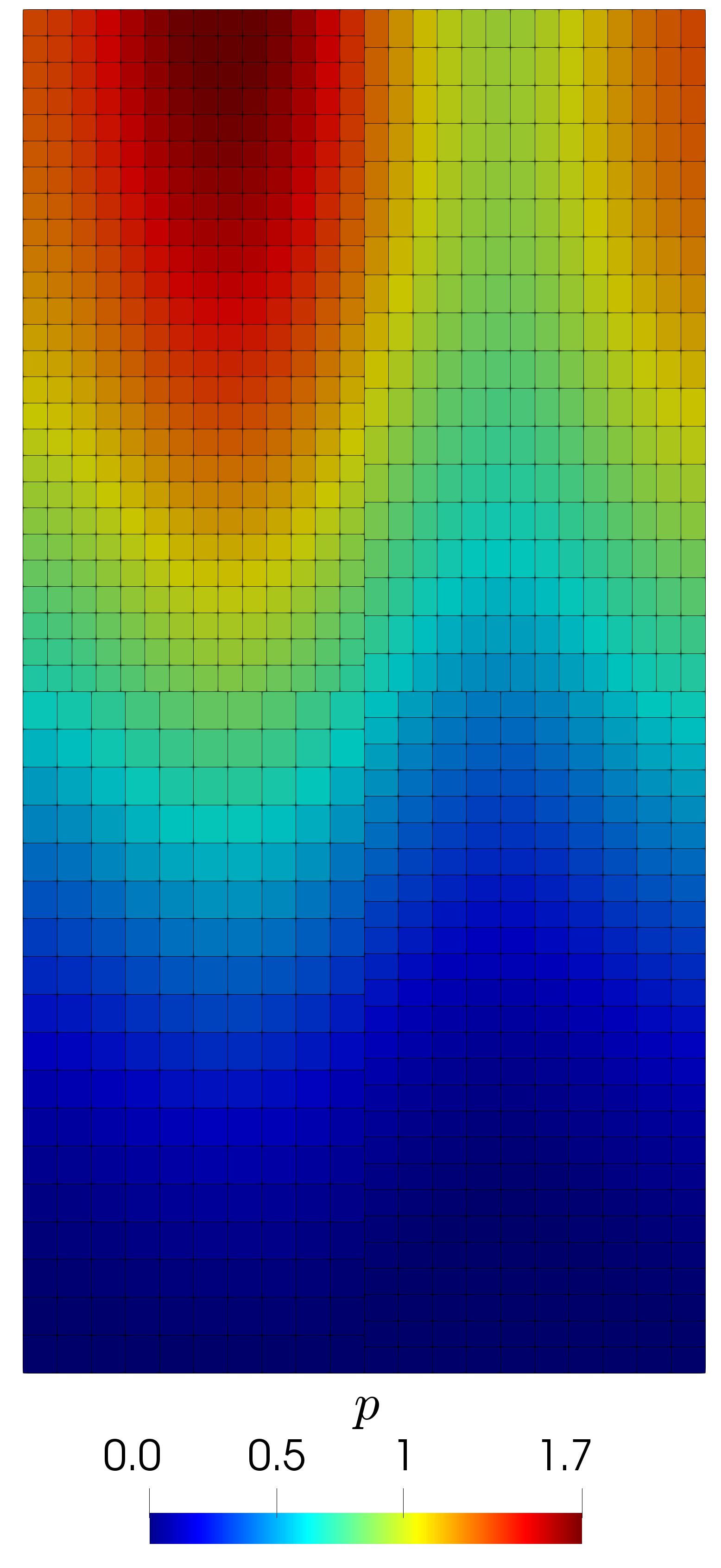
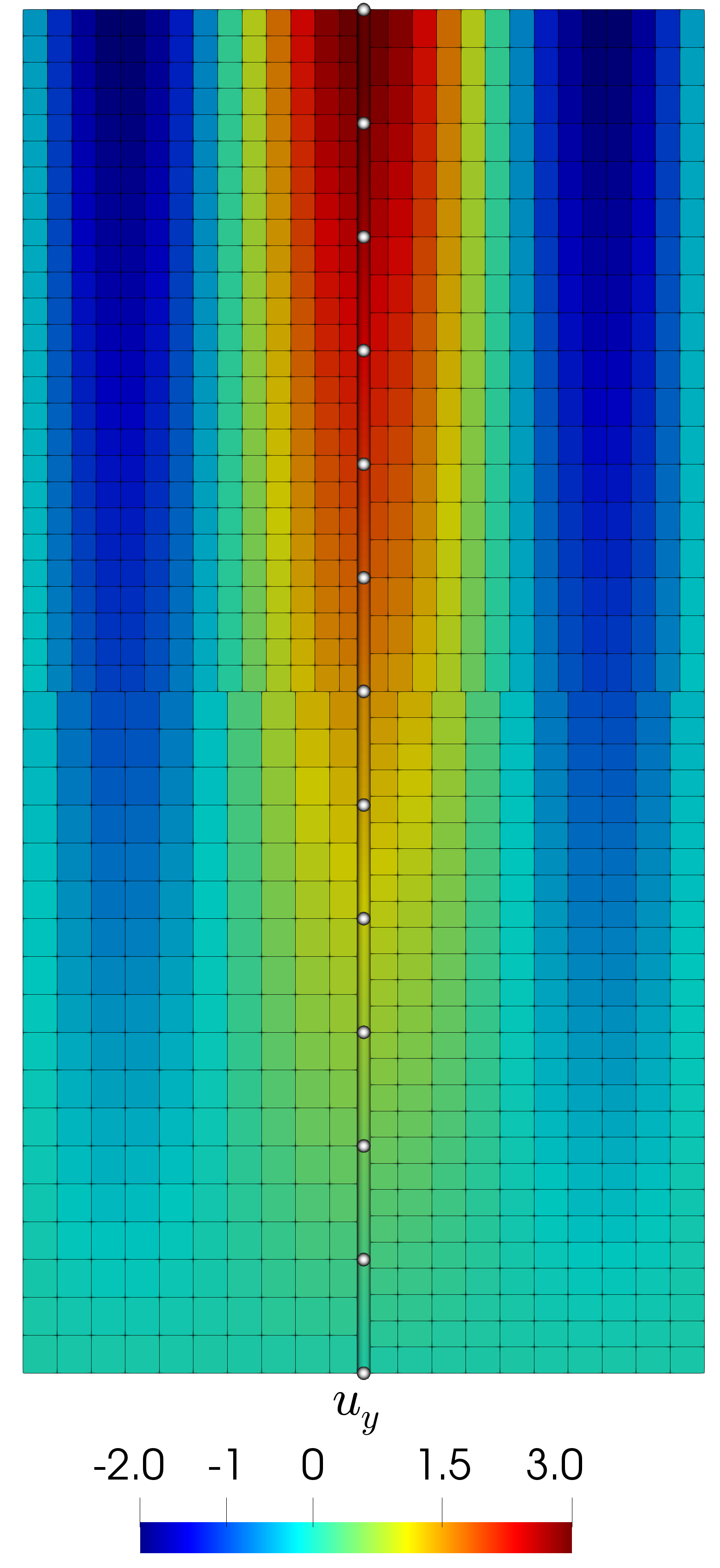
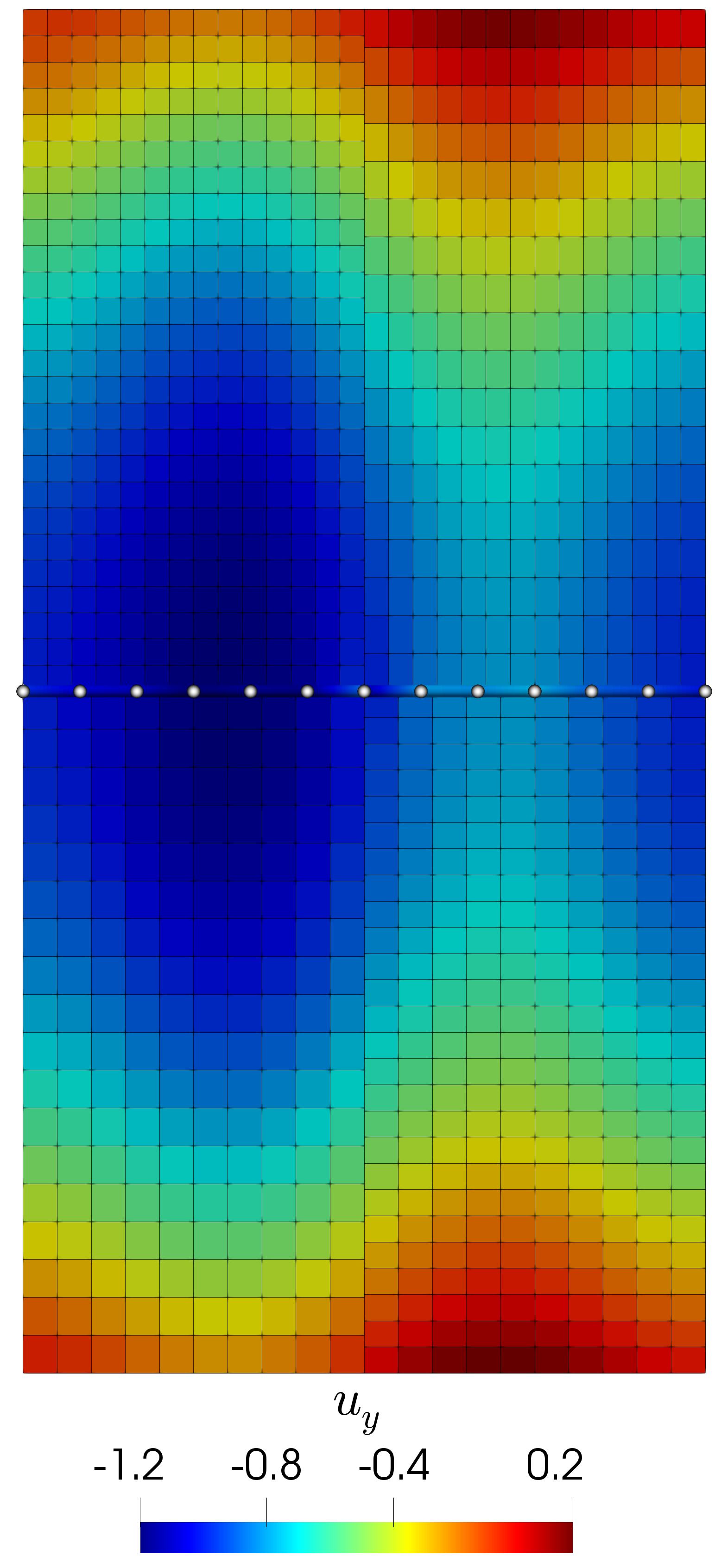
Figure 1: Pressure (left) and velocity (center and right) distributions computed after the first refinement using continuous, piecewise linear mortars ($\mathcal{P}_{1}$) and initial mesh size $h_{\Gamma}^{0}=1/6$. The vertical (center) and horizontal (right) mortar grids are visualized as tubes with white circles indicating the vertices.

We analyze the decrease of the $L^{2}$ errors of the velocity $e_{u}:=\|\bm{u}-\bm{u}_{h}\|_{\Omega}$ , the pressure $e_{p}:=\|p-p_{h}\|_{\Omega}$, the flux-mortar $e_{\lambda}:=\|\lambda-\lambda_{h}\|_{\Gamma}$, and the projected flux-mortar $e_{\mathcal{Q}\lambda}:=\|\lambda-\mathcal{Q}_{h}\lambda_{h}\|_{\Gamma}$. Convergence results for $h_{\Gamma}^{0}=1/4$ are presented in Tables 1 and 2 for $\mathcal{P}_{1}$ and $\mathcal{P}_{0}$ mortars, respectively. The mortar grid is sufficiently coarse and the mortar conditions (3.2) and (3.10) are satisfied. The rates $r_{u}$ and $r_{p}$ indicate first order convergence for the velocity and pressure for both projectors $\mathcal{Q}_{h}^{\flat}$ and $\mathcal{Q}_{h}^{\sharp}$ and both $\mathcal{P}_{1}$ and $\mathcal{P}_{0}$ mortars. We note that the theory predicts $O(h)$ convergence only for $\mathcal{Q}_{h}^{\sharp}$ in the case of $\mathcal{P}_{1}$ mortars, while $O(h^{1/2})$ is predicted in the other cases. The results indicate that consistency error $\mathcal{E}_{c}$, cf. Sections 5.2.1 and 5.2.2, does not have a noticeable influence at these mesh sizes. For the mortar variable, we observe that the rates $r_{\lambda}$ and $r_{\mathcal{Q}\lambda}$ are lower by approximately one half compared to $r_{u}$ and $r_{p}$. This is in agreement with Lemma 5.8.

The most striking observation in both of these tables is that the two extension operators $\mathcal{R}_{h}^{\flat}$ and $\mathcal{R}_{h}^{\sharp}$ produce nearly indistinguishable solutions. However, we have verified numerically that $\mathcal{R}_{h}^{\flat}$ does not produce velocity fields with weakly continuous fluxes across the interfaces, so it is indeed different from $\mathcal{R}_{h}^{\sharp}$. The closeness of the results is another indication that the interface consistency error $\mathcal{E}_{c}$ is dominated by the subdomain discretization error.

Table 1: Errors and convergence rates for $h_{\Gamma}^{0}=1/4$ and $\mathcal{P}_{1}$ mortars.

$\mathcal{P}_{1}$	$e_{u}^{\flat}$	$r_{u}^{\flat}$	$e_{p}^{\flat}$	$r_{p}^{\flat}$	$e_{\lambda}^{\flat}$	$r_{\lambda}^{\flat}$	$e_{\mathcal{Q}\lambda}^{\flat}$	$r_{\mathcal{Q}\lambda}^{\flat}$
0	7.05e-2		4.43e-2		3.78e-2		1.11e-1
1	2.76e-2	1.35	2.18e-2	1.02	1.78e-2	1.08	5.22e-2	1.01
2	1.26e-2	1.14	1.08e-2	1.01	1.13e-2	0.65	2.79e-2	0.91
3	6.11e-3	1.04	5.42e-3	1.00	7.91e-3	0.52	1.59e-2	0.81
4	3.03e-3	1.01	2.71e-3	1.00	5.58e-3	0.50	9.62e-3	0.72
5	1.51e-3	1.00	1.35e-3	1.00	3.95e-3	0.50	6.15e-3	0.64
	$e_{u}^{\sharp}$	$r_{u}^{\flat}$	$e_{p}^{\sharp}$	$r_{p}^{\sharp}$	$e_{\lambda}^{\sharp}$	$r_{\lambda}^{\sharp}$	$e_{\mathcal{Q}\lambda}^{\sharp}$	$r_{\mathcal{Q}\lambda}^{\sharp}$
0	7.05e-2		4.43e-2		3.78e-2		1.05e-1
1	2.76e-2	1.35	2.18e-2	1.04	1.79e-2	1.08	5.23e-2	1.01
2	1.29e-2	1.14	1.08e-2	1.01	1.14e-2	0.65	2.79e-2	0.91
3	6.11e-3	1.04	5.42e-3	1.00	7.92e-3	0.52	1.59e-2	0.81
4	3.03e-3	1.01	2.71e-3	1.00	5.59e-3	0.50	9.62e-3	0.72
5	1.51e-3	1.01	1.35e-3	1.00	3.95e-3	0.50	6.15e-3	0.64

Table 2: Errors and convergence rates for $h_{\Gamma}^{0}=1/4$ and $\mathcal{P}_{0}$ mortars.

$\mathcal{P}_{0}$	$e_{u}^{\flat}$	$r_{u}^{\flat}$	$e_{p}^{\flat}$	$r_{p}^{\flat}$	$e_{\lambda}^{\flat}$	$r_{\lambda}^{\flat}$	$e_{\mathcal{Q}\lambda}^{\flat}$	$r_{\mathcal{Q}\lambda}^{\flat}$
0	1.37e-1		4.48e-2		3.41e-1		4.20e-1
1	4.78e-2	1.51	2.18e-2	1.04	1.70e-1	1.01	2.06e-1	1.03
2	1.85e-2	1.37	1.08e-2	1.01	8.56e-2	0.99	1.03e-1	0.99
3	7.91e-3	1.23	5.42e-3	1.00	4.49e-2	0.93	5.41e-2	0.93
4	3.72e-3	1.09	2.71e-3	1.00	2.62e-2	0.77	3.18e-2	0.76
5	1.92e-3	0.96	1.35e-3	1.00	1.88e-2	0.48	2.33e-2	0.45
	$e_{u}^{\sharp}$	$r_{u}^{\flat}$	$e_{p}^{\sharp}$	$r_{p}^{\sharp}$	$e_{\lambda}^{\sharp}$	$r_{\lambda}^{\sharp}$	$e_{\mathcal{Q}\lambda}^{\sharp}$	$r_{\mathcal{Q}\lambda}^{\sharp}$
0	1.37e-1		4.48e-2		3.41e-1		4.19e-1
1	4.78e-2	1.52	2.18e-2	1.04	1.70e-1	1.01	2.05e-1	1.03
2	1.85e-2	1.37	1.08e-2	1.01	8.56e-2	0.99	1.03e-1	0.99
3	7.91e-3	1.23	5.42e-3	1.00	4.49e-2	0.93	5.40e-2	0.93
4	3.72e-3	1.09	2.71e-3	1.00	2.62e-2	0.77	3.18e-2	0.76
5	1.92e-3	0.96	1.35e-3	1.00	1.88e-2	0.48	2.33e-2	0.45

In Table 3, we show the errors and convergence rates in the case of finer mortar grids with $h_{\Gamma}^{0}=1/6$. The results are only shown for piecewise linear mortars and the projection operator $\mathcal{Q}_{h}^{\flat}$, since the other cases produce similar errors and rates. We observe a deterioration in the rates $r_{\lambda}$ and $r_{\mathcal{Q}\lambda}$. To illustrate this effect, we show in Figure 2 the mortar solution $\lambda_{h}$ obtained on refinement level 5 with the coarser mortar grid $h_{\Gamma}^{0}=1/4$ and the finer mortar grid $h_{\Gamma}^{0}=1/6$. We first note that in both cases an oscillation appears at the junction of the two mortar grids. It is likely due to the Gibbs phenomenon at the end points of the interfaces, since we allow for discontinuity from one interface to another. This oscillation is localized and it does not affect the global accuracy. However, in the finer mortar grid case, an oscillation is also observed along the entire interface. This indicates that the mortar condition (3.2) may be violated in this case. On the other hand, the variables $u_{h}$ and $p_{h}$ appear unaffected by these oscillations and exhibit first order convergence in Table 3.

Table 3: Errors and convergence rates for $h_{\Gamma}^{0}=1/6$ and $\mathcal{P}_{1}$ mortars.

$\mathcal{P}_{1}$	$e_{u}^{\flat}$	$r_{u}^{\flat}$	$e_{p}^{\flat}$	$r_{p}^{\flat}$	$e_{\lambda}^{\flat}$	$r_{\lambda}^{\flat}$	$e_{\mathcal{Q}\lambda}^{\flat}$	$r_{\mathcal{Q}\lambda}^{\flat}$
0	7.08e-2		4.43e-2		4.51e-2		1.10e-1
1	2.82e-2	1.33	2.18e-2	1.03	3.37e-2	0.42	6.37e-2	0.79
2	1.30e-2	1.13	1.08e-2	1.01	2.41e-2	0.48	3.90e-2	0.71
3	6.31e-3	1.03	5.42e-3	1.00	1.74e-2	0.47	2.55e-2	0.61
4	3.15e-3	1.00	2.71e-3	1.00	1.29e-2	0.43	1.78e-2	0.52
5	1.60e-3	0.98	1.35e-3	1.00	9.91e-3	0.38	1.34e-2	0.42

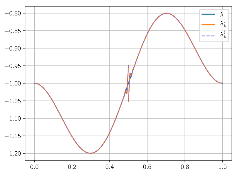
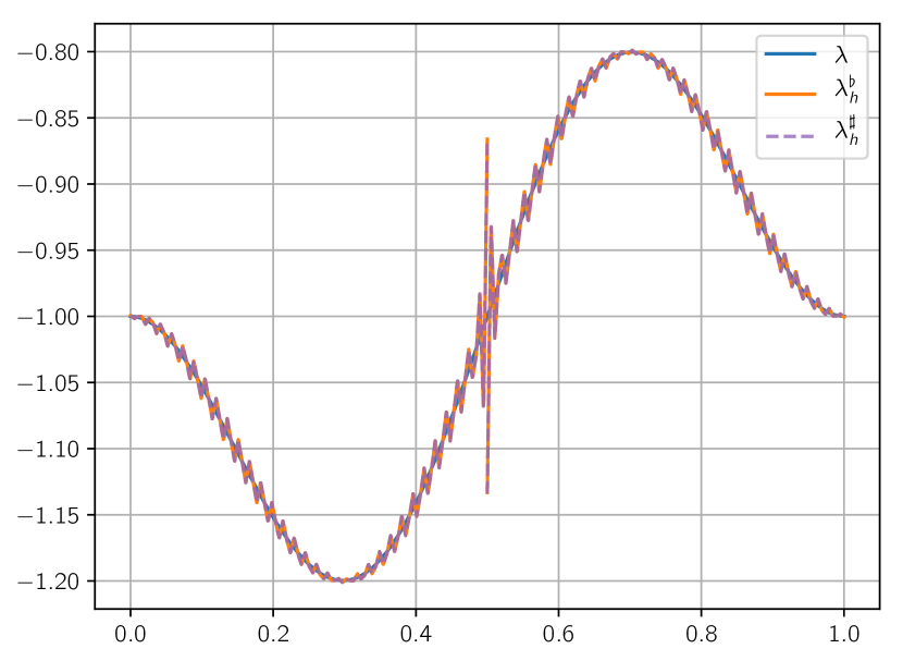
Figure 2: Plot of the true flux $\lambda$ and the discrete flux-mortar solution $\lambda_{h}$ along the line $y=1$, on refinement level 5 with initial mortar mesh size of $h_{\Gamma}^{0}=1/4$ (left) and $h_{\Gamma}^{0}=1/6$ (right).

References

• [1] R. Araya, C. Harder, D. Paredes, and F. Valentin, Multiscale hybrid-mixed method, SIAM J. Numer. Anal., 51 (2013), pp. 3505–3531, https://doi.org/10.1137/120888223.
• [2] T. Arbogast, Analysis of a two-scale, locally conservative subgrid upscaling for elliptic problems, SIAM J. Numer. Anal., 42 (2004), pp. 576–598, https://doi.org/10.1137/S0036142902406636.
• [3] T. Arbogast, L. C. Cowsar, M. F. Wheeler, and I. Yotov, Mixed finite element methods on nonmatching multiblock grids, SIAM J. Numer. Anal., 37 (2000), pp. 1295–1315, https://doi.org/10.1137/S0036142996308447.
• [4] T. Arbogast, G. Pencheva, M. F. Wheeler, and I. Yotov, A multiscale mortar mixed finite element method, Multiscale Model. Simul., 6 (2007), pp. 319–346, https://doi.org/10.1137/060662587.
• [5] M. Arshad, E.-J. Park, and D.-w. Shin, Analysis of multiscale mortar mixed approximation of nonlinear elliptic equations, Comput. Math. Appl., 75 (2018), pp. 401–418, https://doi.org/10.1016/j.camwa.2017.09.031.
• [6] F. Ben Belgacem, The mixed mortar finite element method for the incompressible Stokes problem: convergence analysis, SIAM J. Numer. Anal., 37 (2000), pp. 1085–1100 (electronic), https://doi.org/10.1137/S0036142997329220.
• [7] D. Boffi, F. Brezzi, and M. Fortin, Mixed finite element methods and applications, vol. 44, Springer, 2013.
• [8] W. M. Boon, A parameter-robust iterative method for Stokes-Darcy problems retaining local mass conservation, ESAIM Math. Model. Numer. Anal., (2020), https://doi.org/10.1051/m2an/2020035.
• [9] W. M. Boon, J. M. Nordbotten, and I. Yotov, Robust discretization of flow in fractured porous media, SIAM J. Numer. Anal., 56 (2018), pp. 2203–2233, https://doi.org/10.1137/17M1139102.
• [10] S. C. Brenner, Korn’s inequalities for piecewise H1 vector fields, Math. Comp., (2004), pp. 1067–1087.
• [11] M. Discacciati, E. Miglio, and A. Quarteroni, Mathematical and numerical models for coupling surface and groundwater flows, Appl. Numer. Math., 43 (2002), pp. 57–74. 19th Dundee Biennial Conference on Numerical Analysis (2001).
• [12] M. Discacciati, A. Quarteroni, and A. Valli, Robin-Robin domain decomposition methods for the Stokes-Darcy coupling, SIAM J. Numer. Anal., 45 (2007), pp. 1246–1268 (electronic), https://doi.org/10.1137/06065091X.
• [13] B. Flemisch, M. Darcis, K. Erbertseder, B. Faigle, A. Lauser, K. Mosthaf, S. Müthing, P. Nuske, A. Tatomir, M. Wolff, and R. Helmig, Dumux: Dune for multi- {Phase, Component, Scale, Physics, …} flow and transport in porous media, Advances in Water Resources, 34 (2011), pp. 1102–1112, https://doi.org/10.1016/j.advwatres.2011.03.007.
• [14] G. P. Galdi, An introduction to the mathematical theory of the Navier-Stokes equations. Vol. I, Springer-Verlag, New York, 1994. Linearized steady problems.
• [15] J. Galvis and M. Sarkis, Non-matching mortar discretization analysis for the coupling Stokes-Darcy equations, Electron. Trans. Numer. Anal., 26 (2007), pp. 350–384.
• [16] J. Galvis and M. Sarkis, FETI and BDD preconditioners for Stokes-Mortar-Darcy systems, Commun. Appl. Math. Comput. Sci., 5 (2010), pp. 1–30.
• [17] B. Ganis and I. Yotov, Implementation of a mortar mixed finite element method using a multiscale flux basis, Comput. Methods Appl. Mech. Engrg., 198 (2009), pp. 3989–3998, https://doi.org/10.1016/j.cma.2009.09.009.
• [18] V. Girault, D. Vassilev, and I. Yotov, Mortar multiscale finite element methods for Stokes-Darcy flows, Numer. Math., 127 (2014), pp. 93–165, https://doi.org/10.1007/s00211-013-0583-z.
• [19] R. Glowinski and M. F. Wheeler, Domain decomposition and mixed finite element methods for elliptic problems, in First International Symposium on Domain Decomposition Methods for Partial Differential Equations, R. Glowinski, G. H. Golub, G. A. Meurant, and J. Periaux, eds., SIAM, Philadelphia, 1988, pp. 144–172.
• [20] C. Harder, D. Paredes, and F. Valentin, A family of multiscale hybrid-mixed finite element methods for the Darcy equation with rough coefficients, J. Comput. Phys., 245 (2013), pp. 107–130, https://doi.org/10.1016/j.jcp.2013.03.019.
• [21] E. Khattatov and I. Yotov, Domain decomposition and multiscale mortar mixed finite element methods for linear elasticity with weak stress symmetry, ESAIM Math. Model. Numer. Anal., 53 (2019), pp. 2081–2108, https://doi.org/10.1051/m2an/2019057.
• [22] H. H. Kim and C.-O. Lee, A Neumann-Dirichlet preconditioner for a FETI-DP formulation of the two-dimensional Stokes problem with mortar methods, SIAM J. Sci. Comput., 28 (2006), pp. 1133–1152, https://doi.org/10.1137/030601119.
• [23] T. Koch, D. Gläser, K. Weishaupt, S. Ackermann, M. Beck, B. Becker, S. Burbulla, H. Class, E. Coltman, S. Emmert, T. Fetzer, C. Grüninger, K. Heck, J. Hommel, T. Kurz, M. Lipp, F. Mohammadi, S. Scherrer, M. Schneider, G. Seitz, L. Stadler, M. Utz, F. Weinhardt, and B. Flemisch, DuMux 3 - an open-source simulator for solving flow and transport problems in porous media with a focus on model coupling, Comput. Math. with Appl., (2020), https://doi.org/10.1016/j.camwa.2020.02.012.
• [24] W. J. Layton, F. Schieweck, and I. Yotov, Coupling fluid flow with porous media flow, SIAM J. Numer. Anal., 40 (2002), pp. 2195–2218 (2003), https://doi.org/10.1137/S0036142901392766.
• [25] J. Li and O. Widlund, BDDC algorithms for incompressible Stokes equations, SIAM J. Numer. Anal., 44 (2006), pp. 2432–2455, https://doi.org/10.1137/050628556.
• [26] J. M. Nordbotten, W. M. Boon, A. Fumagalli, and E. Keilegavlen, Unified approach to discretization of flow in fractured porous media, Computational Geosciences, 23 (2019), pp. 225–237.
• [27] L. F. Pavarino and O. B. Widlund, Balancing Neumann-Neumann methods for incompressible Stokes equations, Comm. Pure Appl. Math., 55 (2002), pp. 302–335, https://doi.org/10.1002/cpa.10020.
• [28] G. Pencheva and I. Yotov, Balancing domain decomposition for mortar mixed finite element methods, Numer. Linear Algebra Appl., 10 (2003), pp. 159–180, https://doi.org/10.1002/nla.316.
• [29] M. Peszyńska, M. F. Wheeler, and I. Yotov, Mortar upscaling for multiphase flow in porous media, Comput. Geosci., 6 (2002), pp. 73–100, https://doi.org/10.1023/A:1016529113809.
• [30] A. Quarteroni and A. Valli, Domain decomposition methods for partial differential equations, Oxford University Press, 1999.
• [31] A. Quarteroni and A. Valli, Numerical approximation of partial differential equations, vol. 23, Springer Science & Business Media, 2008.
• [32] L. R. Scott and S. Zhang, Finite element interpolation of nonsmooth functions satisfying boundary conditions, Math. Comput., 54 (1990), pp. 483–493, https://doi.org/10.2307/2008497.
• [33] R. Stenberg, Analysis of mixed finite elements methods for the Stokes problem: a unified approach, Math. Comp., 42 (1984), pp. 9–23, https://doi.org/10.2307/2007557.
• [34] A. Toselli and O. Widlund, Domain decomposition methods—algorithms and theory, vol. 34 of Springer Series in Computational Mathematics, Springer-Verlag, Berlin, 2005.
• [35] D. Vassilev, C. Wang, and I. Yotov, Domain decomposition for coupled Stokes and Darcy flows, Comput. Methods Appl. Mech. Engrg., 268 (2014), pp. 264–283, https://doi.org/10.1016/j.cma.2013.09.009.