An Edge-powered Approach to Assisted Driving
Abstract
Automotive services for connected vehicles are one of the main fields of application for new-generation mobile networks as well as for the edge computing paradigm. In this paper, we investigate a system architecture that integrates the distributed vehicular network with the network edge, with the aim to optimize the vehicle travel times. We then present a queue-based system model that permits the optimization of the vehicle flows, and we show its applicability to two relevant services, namely, lane change/merge (representative of cooperative assisted driving) and navigation. Furthermore, we introduce an efficient algorithm called Bottleneck Hunting (BH), able to formulate high-quality flow policies in linear time. We assess the performance of the proposed system architecture and of BH through a comprehensive and realistic simulation framework, combining ns-3 and SUMO. The results, derived under real-world scenarios, show that our solution provides much shorter travel times than when decisions are made by individual vehicles.
I Introduction
Vehicle traffic congestion has been identified as a prime cause of road accidents, with their significant cost in term of time and lives [1]. Among the strategies to alleviate congestion, coordination between vehicles has been studied in several contexts, including lane maneuvers [2], intersection management [3], and traffic light optimization [4]. The emergence of connected vehicles, with their assisted- and self-driving capabilities, has fostered further interest in this topic, as witnessed by European projects [5, 6, 7] and international standards [8].
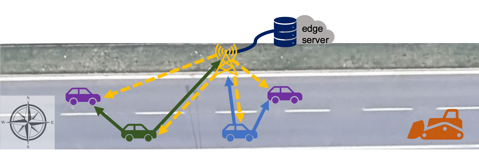
However, present-day research efforts envision that vehicles make local decisions, and aim at providing such vehicles with as much information as possible. In view of the fact that local decisions have far-reaching consequences on the global traffic flow, we envision an alternative system architecture, based on the edge computing paradigm and summarized in Fig. 1, where:
-
•
an edge server formulates policies, concerning all traffic flows;
-
•
actualizers located at the infrastructure, e.g., cellular eNBs or road-side units (RSUs) translate such policies into local, per-vehicle decisions.
With reference to Fig. 1, a policy may dictate that 60% of vehicle traveling on the south lane should turn left early (where the green vehicle is), and the rest later (where the blue vehicle is). Given this policy, actualizers can give advice to individual vehicles, chosen randomly according to a 60%-40% proportion, on when to change lanes.
Formulating the policies at the edge server is not an easy task, for several reasons. First, policies need to account for how vehicles with different destinations sharing the same stretch of road influence each other’s travel times. Second, in order to ensure fairness, it is not enough to optimize the average travel time of vehicles with a given source and destination, rather the travel time distribution over all vehicles needs to be considered. Third, all such decisions must be made effectively – optimally, if possible – and efficiently, in order to quickly react to changes in the vehicle traffic.
In this paper, we address the task of formulating policies at the edge server, by making the following main contributions:
-
•
introducing a system architecture, detailed in Sec. II, combining the distributed vehicular network with an edge-based decision-maker, whose task is to formulate traffic flow-level policies;
-
•
proposing, in Sec. III, a queue model describing arbitrary road topologies, the paths taken by vehicles, and the distribution of their travel times, in a tractable manner;
- •
-
•
presenting, in Sec. VI, an optimal algorithm with linear complexity, called Bottleneck Hunting (BH), along with a discussion on its novelty with respect to traditional multi-path packet routing.
The performance evaluation results, obtained through the methodology outlined in Sec. VII and summarized in in Sec. VIII, confirm that the policies formulated by BH result in much shorter travel times than the decisions made by individual vehicles. Finally, after reviewing related work in Sec. IX, we conclude the paper in Sec. X.
II System architecture
We now introduce our new architecture, highlighting how it is consistent with existing standards on connected vehicle communications. According to the ETSI 102.941 (2019) standard, connected vehicles periodically (e.g., every 100 ms) broadcast cooperative awareness messages (CAMs), including their location, speed, and heading. Such information is then used by other vehicles and/or the network infrastructure for several safety and convenience services, e.g., [9]. Upon detecting a situation warranting action, decentralized environmental notification messages (DENMs) are sent to the affected vehicles, so that their actuator is triggered and/or their driver is warned. Both CAMs and DENMs can carry additional information [8] for the support of assisted driving services such as lane change/merge [8] and navigation services (see ETSI 102.638).
None of the above is envisioned to change under our proposed architecture; in particular, all services still leverage the transmission of CAMs and DENMs. For concreteness, we focus on the lane change assistance and navigation services. In the first case, the edge server exploits the information in the CAMs received by the radio access nodes (and possibly notifications of lane blocks carried by DENMs) to formulate an optimal policy. Such a policy is then sent to the actualizers, which, being closer to the mobile users, can account for the most recent CAMs and exploit them to translate the policy into individual instructions for the single vehicles (see Fig. 1). These instructions are notified to vehicles through DENMs sent by the radio access nodes. Upon receiving a DENM, a vehicle starts interacting via V2V communications with its neighbors following, e.g., the protocol defined in [5] and using CAMs and DENMs as foreseen by [8].
The second service (navigation) operates on a longer time and geographical scale: the edge server exploits the CAMs and, in particular, the route destination field therein, and computes the optimal vehicles’ route. This is then notified by the radio access nodes using DENMs.
III Model design
In this section, we describe how our system model represents the road layout, the vehicle flows (Sec. III-A), the routes taken by vehicles in the same flow, and their travel times (Sec. III-B). Importantly,
-
•
based on the existing works and validation studies (see Sec. IX), we consider Markovian arrivals, of either individual vehicles or batches thereof;
-
•
we do not restrict ourselves to a specific service time distribution, i.e., consider generic MX/G/1 queues;
-
•
given the scope of our work, we focus on uncongested scenarios where the number of vehicles traveling on a road stretch is lower than its capacity, hence road stretches can be modeled with queues with infinite length.
The decisions to be made correspond, intuitively, to the policies formulated by the edge server in Fig. 1. Specifically, they consist of the suggested travel speed and the probabilities of taking a given lane/stretch of road. In the following, we refer to a single lane on a stretch of road as road segment.
III-A Road topologies as queue networks
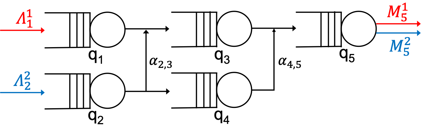
We model the road topology under the control of the edge server as a set of interconnected queues , as exemplified in Fig. 2. Similarly to existing works (including experimental validation, see Sec. IX), each queue represents a road segment, characterized, e.g., by a certain speed limit and capacity.
Service rates, , are bounded by a maximum value , determined by the length of the road segment modelled by queue , its speed limit, and the inter-vehicle safety distance:
| (1) |
Several traffic flows, , may travel across the road topology or part of it, each flow being defined as a set of vehicles having the same source and destination within the road topology. Specifically, given a flow entering and leaving the road topology at queue and , respectively, the parameter denotes the vehicles arrival rate, while parameter denotes the rate at which they exit the topology. Notice that, for every flow , there will be exactly one queue for which and one for which (see Fig. 2). Vehicles move from a generic queue to a queue according to probability .
Given the above model, our decision variables are the service rates of queues , and the transition probabilities (although some can be fixed, e.g., in Fig. 2, ). The total incoming flow for queue is denoted with and depends on , , , and the probability that queue is empty:
| (2) |
Eq. (2) can be read as follows: the flow incoming into queue is equal to the flow of vehicles that begin their journey therein, plus a fraction of the vehicles that exit other queues , but do not leave yet the road topology.
III-B A path-based view
Vehicles of the same flow, i.e., having the same source and the same destination within the road topology, may nonetheless have different trajectories, hence, traverse different sequences of queues. We define such sequences of queues as paths . Each path is an array including the queues traversed by vehicles taking it; given a queue , we write if path includes . The probability that vehicles of flow take path is denoted by ; each path is used by one flow only, indicated as . Introducing paths allows for a flexible relationship between flows and queues, thus enhancing the realism of our model, while keeping its computational complexity low.
Importantly, given the edge-based policy, vehicles are assigned a path (according to the probabilities) at the beginning of their travel across the considered road topology, before they enter the first queue. Thus, given the path it takes, the queues traversed by a vehicle are unequivocally determined.
The probabilities that vehicles of flow take path can be expressed as a function of the probabilities as follows:
| (3) |
where is the -th queue included in path . Clearly, the probabilities have to sum up to one:
| (4) |
We stress that, while each path is unequivocally associated with one flow, the opposite does not hold. With reference to Fig. 2, flow is associated with one path only, while flow can use path or . As for paths and queues, there is a many-to-many relationship between them. In Fig. 2, queues and belong to one path each, queues and to two paths each, and queue to all three paths.
When considering paths, the local arrival rate at each queue in (2) depends on: the paths belongs to, the probability that flows take those paths, and the arrival rate of those flows. Specifically,
| (5) |
IV Path Travel Times
In the following, we leverage the path-based view of the system to characterize the travel time experienced by each flow . Let us first denote with the probability density function (pdf) of the sojourn time at an individual queue . Such pdf is a function of and , according to an expression that depends on the statistics of the queue arrival process and the service time. Then, recalling that vehicles taking path traverse all queues in , the travel time associated with path is the sum of the sojourn times at all queues therein. The pdf of such a time is the -way convolution of the individual pdfs associated with each queue, i.e., . By integrating , we compute the cumulative density functions (CDFs) and take their Laplace transform, thus obtaining:
| (6) |
where is the Laplace transform of .
Anti-transforming, we can obtain the CDF of the path-wise travel time: . We recall that is a function of the control variables and (i.e., ), which appear in the pdf . As mentioned, the actual form of and , as well as of the above Laplace transforms, depends on the queue arrival process and service time distribution. In many cases of interest, can be expressed as a ratio between polynomials, and anti-transformed into a summation of terms of type .
Next, we move from paths to flows. To this end, can be exploited to write the probability that the travel time of a vehicle taking path exceeds a value :
| (7) |
We now need a flow-wise equivalent of . This however cannot be computed using the CDF of the per-flow travel time, i.e., similarly to (7), because such a distribution, in general, is not a linear combination of the path-wise CDFs. Instead, we proceed as follows.
Let be a flow-wise target travel time, e.g., the ratio of the distance between the flow source and destination to the desired average speed between them. Given the value, a good measure of the flow quality of service is given by the probability that the travel time of the vehicles of flow exceeds . To express such values, we can combine the path-wise probabilities in (7) with the values , expressing the probability that a vehicle of flow takes path , and write:
| (8) |
V Problem formulation
Our high-level goal is to keep the fraction of vehicles of each flow , whose travel time exceeds the target , as low as possible. To ensure fairness among vehicles of different flows, we formulate such a goal as the following min-max objective:
| (9) |
The optimization variables are the probabilities (hence the ) and the service rates , which appear in the objective function in (9) via the CDF in (6). Ingress and egress rates and are input parameters, as are the maximum service rates and the target flow travel times . The per-queue arrival rates are auxiliary variables, whose dependency on the decision variables is specified in (5). Furthermore, we need to impose the constraints in (1) and (4).
Reconstructing the -values. Given the optimal values, the variables can be recovered by solving a system of equations of the type of (3), where the -values are the unknown and the -values are given. The system can be linearized by taking the logarithm of all variables, i.e., re-writing (3) as: , .
The fact that the system has a unique solution is ensured by the proposition below; the intuition behind it is that the number of paths grows faster than the number of junctions, hence, there are more equations than variables. Thus, if it exists, the solution is unique.
Solving the problem and finding the optimal value for the values could, in principle, be attempted with commercial, off-the-shelf solvers like CPLEX or Gurobi, at least when a closed-form expression of (9) exists. However, numerical solvers encounter significant numerical difficulties when dealing with the objective (9). Indeed, coefficients therein usually contain a ratio of products of terms: a small variation in any of the terms can change the sign of the whole coefficient and/or significantly alter its (absolute) value. The issue is compounded by the fact that such values, which can be very large, are then multiplied in (8) by probabilities , which could be very small and/or be varied by very small quantities.
To avoid these issues, as well as to leverage problem-specific insights to obtain shorter solution times, we develop instead our own algorithm to solve the problem, as set forth next.
VI The BH algorithm
Our algorithm, named bottleneck-hunting (BH), solves the problem specified in Sec. V with the same worst-case complexity and convergence properties of gradient-based alternatives, but with faster average-case performance. Such a faster convergence is achieved by leveraging problem-specific knowledge and information in order to reduce the number of solutions to try out, hence, of algorithm iterations.
With reference to Alg. 1, at every iteration, BH moves a fraction of flow ’s traffic from path to path . The fraction changes across iterations, and is initialized (Line 1) to a value . Then, at every iteration, BH identifies (Line 3) a set CQ of critical queues, that is, queues that: (i) belong to two paths and ; (ii) are not the most loaded queue in ; and, (iii) increasing their load by a fraction of the traffic of flow renders it the most loaded queue in . It follows that the algorithm will try to avoid routing additional traffic on critical queues in CQ if possible. Based on CQ, a set CP of critical paths, i.e., paths containing at least one critical queue, is identified in Line 4.
Next, BH identifies the set FA of flows that can be acted upon. Flows using at least one non-critical path are tried first (Line 5); if no such flow exists (Line 6), then FA is extended to include all flows in (Line 7). The flow to act upon is chosen in Line 8: considering the min-max nature of objective (9), is the flow for which the summation in (9) is largest. For the same reason, the path to remove vehicles from is chosen as the most loaded one, hence, the one associated with the largest term in (9). Similarly, the path to add traffic to is selected (Line 10) as the least-loaded one among those used by ; note that this implies choosing a non-critical path if such paths exist.
In Line 11, BH calls the function does_improve, which recomputes (9) and checks whether it improves by moving a fraction of ’s vehicles from path to path . Indeed, the objective may not improve if the current value of is too high, i.e., moving a fraction of traffic increases the traffic intensity on too much. In this case, such action should be performed at a later iteration, when will be smaller (Line 15). If the objective improves, the variables are updated accordingly, in Line 12–Line 13. The algorithm terminates when drops below the minimum value (Line 16).
VII Validation Methodology
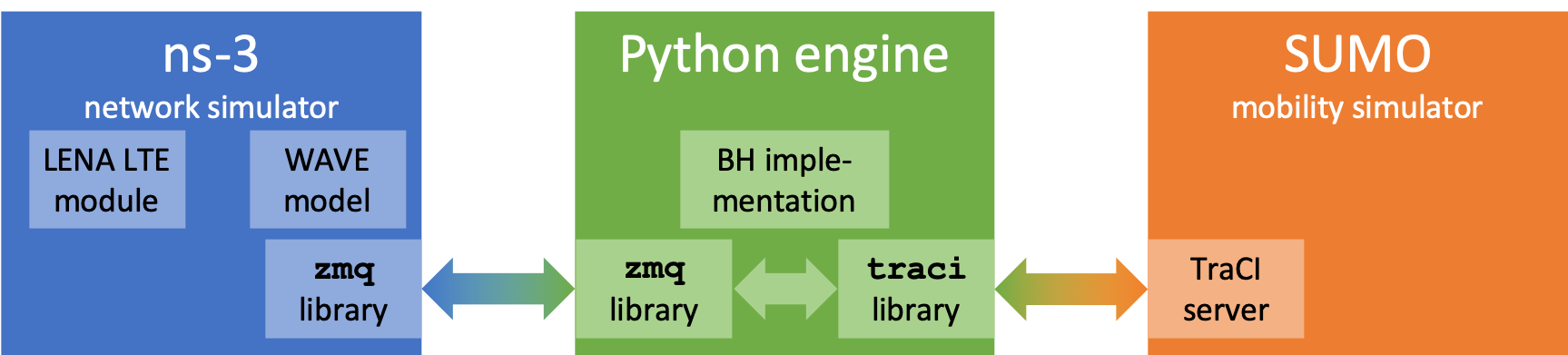
To assess its performance, we integrate BH within a complete validation environment, as represented in Fig. 3. Policies summarized by the and variables are defined by BH, implemented within a Python engine. Such decisions are then relayed to the ns-3 network simulator, which is in charge of: (i) simulating the network traffic generated by vehicles and by the infrastructure, and (ii) based on the most recent CAMs, implementing the edge-defined policy while minimizing the disruption for the vehicles.
In the case of the lane-change service, upon receiving a DENM, vehicles engage their neighbors in a communication following the protocol in [5], to coordinate their manoeuvers and avoid collisions. As a consequence, the target vehicle as well as its neighbors may vary their trajectory, and such a variation may have cascade effects on the mobility of other vehicles. All mobility, in both the lane-change and the navigation case, is simulated via SUMO. Based on the SUMO simulation, the position of each vehicle is then updated within ns-3.
The mobility information is relayed between ns-3 and SUMO through the Python engine and the TraCI Python library. The ns3 simulator and the Python engine interact through the zmq message-passing framework, using the client libraries available for both Python and C++. The communication between SUMO and the Python engine, instead, takes place through the TraCI protocol.
In SUMO, flows include a mixture of different vehicle types, namely cars (SUMO class passenger, 85% of all vehicles), trucks (class truck, 10% of vehicles), and buses (class coach, 5% of vehicles). Their target speed, acceleration, and driving aggressiveness values are left to the SUMO default, subject to a global speed limit of 50 km/h, as it is common in urban areas. The simulation step size of SUMO, which also determines the frequency of position updates in ns-3, is set to 10 ms.
In ns-3, LTE (provided by the LENA module) is used for the communication between vehicles and infrastructure, while WAVE (in the default ns-3 distribution) is used for V2V communication, including that required for lane change. CAMs and DENMs are encoded as foreseen by the ETSI 302.637 standard for ITS. Upon receiving a DENM, vehicles take action immediately, which corresponds to the case of autonomous vehicles. Human reaction times, usually quantified in 1 s [9], could be easily accounted for.
VIII Numerical Results
We now demonstrate how our system model and the BH algorithm can be exploited, by considering a lane-change service in the small-scale scenario described in Fig. 1 and modelled in Fig. 2. Therein, there are two incoming flows, namely, flows 1 and 2: the former is associated with one path only, the latter with two paths. These two paths are called early and late, referring to the fact that vehicles turn north (respectively) after the first road segment (i.e., ), or after the second one (i.e., ). We set the normalized111Rates are normalized to the arrival rate of flow 1. incoming rate to for both flows, and the maximum normalized service rate to for all road segments, except for that, owing to the fact that vehicles therein need to slow down, has a maximum normalized service rate . Also, we set to 5 time units for both flows. In such a scenario, the optimal values of coincide with for all road segments, thus the decisions to make are summarized by the variable (indeed, flow 1 only has one path and ).
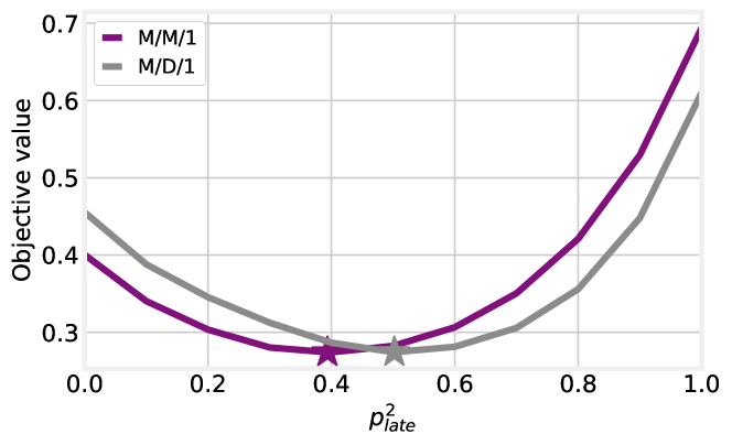
The first, high-level question we seek to answer concerns the relationship between the variable and the value of the objective function (9). Fig. 4 shows that it is advantageous to split the vehicles of flow 2 more or less evenly between its two possible paths.
The third prominent message conveyed by Fig. 4 is about the flexibility of our approach: the purple curve is obtained by modeling road segments as M/M/1 queues, thus using closed-form expressions, while the gray curve is obtained by using M/D/1 queues. Since there is no closed-form expression of the sojourn time distribution in M/D/1 queues, we implemented the approximate formula presented in [10], and solved numerically integrals and convolutions. In spite of the very significant differences with respect to the M/M/1 case, our approach and BH work with no changes in both cases: our solution strategy does not depend on any specific service time distribution, and does not require such a distribution to have a closed-form expression.
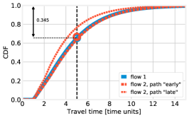
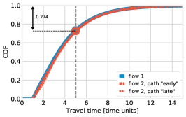
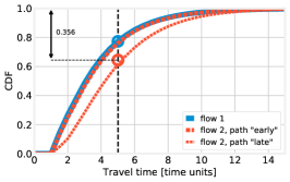
Still for the M/D/1 case, Fig. 5 shows the distribution of the per-path travel times, along with a graphical interpretation of the , , and quantities. Each curve corresponds to a path, and its color represents the flow each path belongs to (namely, blue: flow 1, red: flow 2). Firstly, we observe that, as the intuition would suggest, a higher value of , i.e., sending more vehicles to path late of flow 2, results in longer travel times for that path, and shorter ones for path early. Secondly, the black vertical line in all plots corresponds to the value of the target travel time ; ideally, one would like all CDFs to be at the left of such a line. The intersections between the CDFs and the vertical line represent the probability that vehicles belonging to a flow take a path whose travel time does not exceed , i.e., . Instead, the circles noted on the plots represent the flow-wise performance : as specified in (8), such a quantity is defined as a weighted sum of the values, thus, is close to when most vehicles take path early (left plot), and close to in the opposite case (right plot).
The lowest circle, and the numerical values reported in the plots, correspond to the largest value of , i.e., the value of the objective function in (9): intuitively, optimizing (9) corresponds to pushing up such a circle as high as possible. Note that the flow with the highest changes for different values of : it is flow 1 in the left plot, and flow 2 in the right one. In the center plot, corresponding to the optimal solution, all paths exhibit roughly the same travel time distribution. This is consistent with the intuition we leverage for the design of the BH algorithm: similar path travel times result in better performance.
IX Related work
Queues have been consistently and effectively used to represent vehicular traffic [11]. As early as 1995, [12] argued that vehicles arrive at intersection, either individually or in batches, following a Poisson process. The later work [13] leveraged empirical validation to argue for a more general, M/G/1 model in non-congested scenarios. In both cases, individual lanes are each associated with a queue. Vehicular mobility is modeled through M/M/1 queues also in several recent works about edge and cloud computing in vehicular networks, including [14, 15, 16].
Other works, e.g., [17], focus on specific aspects of vehicular traffic, such as modeling the delay of indisciplined traffic: M/M/1 models are found to accurately represent real-world conditions. Consistently, the study in [18], based on realistic simulations, finds M/M/1 to well represent travel time on individual road segments. Note that part of the popularity of Markovian service times is due to their ability to capture the effect of heterogeneous traffic (e.g., cars, trucks,…) [17], proceeding at different speeds.
Batch arrival and departure processes are the modeling tool of choice when traffic signals are involved, e.g., [19, 20]. In all cases, arrivals are assumed to be Markovian in nature, while service times are either Markovian or deterministic.
Situations where vehicles from multiple flows have to merge into one lane has been identified as a major cause of congestion. Accordingly, several research efforts focus on modeling [21] the merging behavior of vehicles. Recent efforts such as [2] deal with merging strategies for autonomous vehicles, and the benefits coming from cooperation between them. Finally, [22] envisions a centralized controller for merge manoeuvers, accounting for the impact of local merging behaviors on the global traffic conditions.
X Conclusions
We considered assisted driving services for connected vehicles, aiming at optimizing the traffic flows. We first introduced a system architecture that integrates the distributed vehicular network with the edge network, thus enabling edge-controlled traffic flows. Then we developed a queue-based model describing arbitrary road topologies and the behavior of the vehicles traveling through them. Through such a model, we derived the distribution of the vehicle travel times and used it to formulate the problem of optimizing such times. We then devised the BH algorithm, which provides optimal policies in linear time without requiring a closed-form expression for the distribution of the queue service time. Our results, derived through a comprehensive and realistic simulation framework, confirm that the policies formulated by BH result in much shorter travel times than distributed decisions.
Acknowledgments
This work was supported by TIM through the contract “Performance Analysis of Edge Solutions for Automotive Applications”.
References
- [1] World Health Organization. Global status report on road safety.
- [2] M. Zhou et al., “On the impact of cooperative autonomous vehicles in improving freeway merging: a modified intelligent driver model-based approach,” IEEE Trans. on ITS, 2016.
- [3] J. Lehoczky, “Traffic intersection control and zero-switch queues under conditions of markov chain dependence input,” Journal of Applied Probability, 1972.
- [4] M. C. Dunne, “Traffic delay at a signalized intersection with binomial arrivals,” INFORMS Transportation Science, 1967.
- [5] L. Hobert et al., “Enhancements of v2x communication in support of cooperative autonomous driving,” IEEE Comm. Mag., 2015.
- [6] M. Fallgren et al., “Fifth-generation technologies for the connected car: Capable systems for vehicle-to-anything communications,” IEEE Veh. Tech. Mag., 2018.
- [7] A. de la Oliva et al., “5g-transformer: Slicing and orchestrating transport networks for industry verticals,” IEEE Comm. Mag., 2018.
- [8] ETSI, “ETSI 103 299 - v2.1.1,” Tech. Rep., 2019.
- [9] M. Malinverno et al., “Mec-based collision avoidance for vehicles and vulnerable users,” ArXiv preprint 1911.05299, 2019.
- [10] V. Iversen et al., “Waiting time distribution in M/D/1 queueing systems,” IEEE Electronics Letters, 2000.
- [11] T. Van Woensel et al., “Modeling traffic flows with queueing models: A review,” Asia-Pacific Journal of Operational Research (APJOR), 2007.
- [12] A. S. Alfa et al., “Modelling vehicular traffic using the discrete time markovian arrival process,” INFORMS Transportation Science, 1995.
- [13] T. Van Woensel et al., “Empirical validation of a queueing approach to uninterrupted traffic flows,” Springer 4OR, 2006.
- [14] Z. Zhou et al., “Begin: Big data enabled energy-efficient vehicular edge computing,” IEEE Comm. Mag., 2018.
- [15] Z. Ning et al., “Vehicular fog computing: Enabling real-time traffic management for smart cities,” IEEE Wireless Comm., 2019.
- [16] L. Zhao et al., “Joint optimization of communication and traffic efficiency in vehicular networks,” IEEE Trans. on Veh. Tech., 2018.
- [17] S. Mukhopadhyay et al., “Approximate mean delay analysis for a signalized intersection with indisciplined traffic,” IEEE Trans. on ITS, 2017.
- [18] C. Borgiattino et al., “Modelling realistic vehicle traffic flows,” in IEEE SECON VCSC Workshop, 2012.
- [19] R. Timmerman et al., “Platoon forming algorithms for intelligent street intersections,” in Mathematics Applied in Transport and Traffic Systems, 2019.
- [20] E. Harahap et al., “Modeling and simulation of queue waiting time at traffic light intersection,” in IOP Journal of Physics: Conference Series, 2019.
- [21] V. Kanagaraj et al., “Modeling vehicular merging behavior under heterogeneous traffic conditions,” SAGE Transportation Research Record, 2010.
- [22] D. Bushnell, “A merging control system for the urban freeway,” IEEE Trans. on Veh. Tech., 1970.