Phase-resolved analyses of mHz quasi-periodic oscillations in 4U 1636-53 using Hilbert-Huang transform

Abstract

We present phase-resolved spectroscopies based on Hilbert-Huang transform (HHT) for millihertz quasi-periodic oscillations (mHz QPOs) in 4U 1636-536. This $\sim$8 mHz QPO can be detected approximately several thousand seconds before a type-I X-ray burst. It was interpreted as marginally stable burning on the neutron-star surface. In this study, we used HHT to analyze the data collected by XMM-Newton between 2007 and 2009. HHT is a powerful tool that enables us to obtain instantaneous frequency, amplitude and phase of non-stationary periodicity phenomena, such as QPOs. With well-defined phases, the oscillation profile of the $\sim$8 mHz QPO for 4U 1636-53 can be precisely revealed. In addition to the oscillation profile, phase-resolved spectra for the complete cycle are constructed. From the correlation between spectral parameters and fluxes, we find that the oscillation is mainly attributed to the variations of emitting area of blackbody radiation in three out of four observations with mHz QPO detections whereas the other one shows concurrent variation of temperature and flux with a constant emitting area. Although the cause of the difference is not clear, it might be related to the spectral state of the source that can be observed from hard color difference in color-color diagram.

1 Introduction

Various kinds of quasi-period oscillations (QPOs) that exhibit boxer peaks in the power spectra have been observed in many low mass X-ray binaries (LMXBs). These QPOs are believed to reflect phenomena associated with accretion disks (see van der Klis 2006 for extensive review). However, a new kind of QPO, referred to as mHz QPO, was discovered in the accreting neutron star binaries 4U 1636-536 and 4U 1608-52 and was occasionally observed in Aql X-1 (Revnivtsev et al., 2001). Revnivtsev et al. (2001) suggested that these mHz QPOs are caused by a special mode of nuclear burning on the neutron star surface because the flux in 4U 1608-52 was in a narrow range during occurring mHz QPO, that is approximately consistent with the flux in which type-I X-ray bursts cease to exist. However, they did not exclude the possibility that the mHz QPOs were attributed to the instability of the accretion disk. Revnivtsev et al. (2001) also discovered that all mHz QPOs occur before Type-I burst and disappear afterward. Following this discovery, the mHz QPOs were also detected in numerous LMXBs, such as 4U 1323-62 (Strohmayer & Altamirano, 2012), IGR J17480-2446 in Terzan 5 (Linares et al., 2012) and ”Clocked” Burster GS 1826-238 (Strohmayer et al., 2018). Yu & van der Klis (2002) suggested that the kHz QPO frequency in 4U 1608-52 is anticorrelated with the count rate during a mHz QPOs cycle. Because the kHz QPO is related to the Keplerian orbital frequency at the inner edge of the disk, if mHz QPO was produced from the modulation of the disk, the positive correlation between mHz QPO and kHz QPO should have been detected. This finding provides evidence that mHz QPOs comprise a phenomenon that occurs on the neutron star surface instead of the accretion disk. Altamirano et al. (2008) found that the QPO frequency decreases with time during a mHz oscillation until it disappears as Type-I X-ray burst occurs in 4U 1636-53.

Previous studies showed that mHz QPOs associate with nuclear burning on a neutron star surface (Revnivtsev et al., 2001; Altamirano et al., 2008). The fuel of nuclear reaction is obtained from accretion. Therefore, the accretion rate is an important factor for nuclear burning on the neutron star surface. The stable burning indicates that the nuclear burning rate ($\varepsilon_{nuc}$) and cooling rate ($\varepsilon_{cool}$) are balanced, and both depend on temperature and the depth of the fuel layer (Fujimoto et al., 1981; Keek & Heger, 2015). The fuel piled up on the layer is compressed by a strong gravitational force, and then increase temperature and density in the fuel layer. When the ignition condition ($\varepsilon_{nuc}>\varepsilon_{cool}$) is reached, the thermonuclear runaways would occur. The result of thermonuclear runaways makes the luminosity increase in a short time. This phenomenon is called Type-I X-ray burst. Most Type-I X-ray bursts sources have mixed fuel (hydrogen and helium) on the neutron star surface, and the helium burning is ignited by the hydrogen burning. For a high accretion rate ($>11\%\dot{M}_{Edd}$), the accretion provides sufficient fuel to the burning layer. The hydrogen burning dominates in the fuel layer, and helium accumulates on the bottom of the layer. As the helium burning is ignited, the 3$\alpha$ reaction releases more energy and creates more carbon, that enhances the hot CNO cycle. The hydrogen burning also promotes 3$\alpha$ reaction. This burning layer increases $\varepsilon_{nuc}$ further, and then runaway thermonuclear reactions occur while reaching the ignition condition (Galloway & Keek, 2017).

Heger et al. (2007) proposed that the mHz QPO occurs in a special condition between stable and unstable burning, that is referred to as marginal burning. The nuclear reaction rate increases as the temperature in the fuel layer increases, that causes the fuel in the layer being consumed faster than being supplied by the accretion. Thus, the thickness of the burning layer, $y$, decreases. The cooling rate is proportional to $F/y$, where $F$ is the outward flux. The outward flux $F\approx acT^{4}/3\kappa y$, where $a$ is the radiation constant, $c$ is the speed of light and $\kappa$ is the opacity (Bildsten, 1998). Therefore, as the thickness of the burning layer $y$ decreases, the cooling rate increases to reduce the temperature and the nuclear reaction rate. As the rate of fuel being consumed by the nuclear reaction is less than being supplied by the accretion, the thickness of the burning layer $y$ increases, that causes a smaller cooling rate. Therefore, the temperature and nuclear reaction rate increase again. Heger et al. (2007) estimated that it takes about $P\cong\sqrt{t_{therm}t_{acc}}\sim 120$ sec to complete this QPO cycle. According to this model, marginally stable nuclear burning occurs at accretion rate close to the Eddington rate (Bildsten, 1998; Heger et al., 2007). However, the observation results showed that the accretion rates are much lower than the Eddington rate in 4U 1608-52 and 4U 1636-536 (Revnivtsev et al., 2001). Keek et al. (2009) attempted to find a possible solution by mixing processes. Furthermore, the width of the interval of the accretion rates between stable and unstable nuclear burning strongly depends on the composition of the layer and reaction rates (Keek et al., 2014).

Lyu et al. (2014) and Lyu et al. (2015) analyzed the mHz QPOs in 4U1636-536 using XMM-Newton observations. They also observed the drift in the QPO frequency, that is positively correlated with the temperature of the blackbody component from the neutron star surface. Such drifts could be caused by the cooling of the burning layers. By analyzing 39 Type-I X-ray bursts and mHz QPO in 4U 1636-536, Lyu et al. (2016) determined that the mHz QPO can only be detected when the convexity of the corresponding Type-I X-ray burst is positive. According to the model proposed by Maurer & Watts (2008) and Cooper & Narayan (2007), the convexity links to the ignition site of the bursts on the neutron-star surface. Lyu et al. (2016) suggested that the marginally stable nuclear burning process may occur at the neutron-star equator. Through phase-resolved spectroscopy of mHz oscillations of 4U 1636-536, Stiele et al. (2016) concluded that the mHz QPOs are caused by a variable surface area of nuclear burning on neutron star surface with constant temperature. Nevertheless, Strohmayer et al. (2018) detected the oscillation of the blackbody temperature component in an effectively constant emitting area in 8 mHz QPO of GS 1826-238.

Phase-resolved analysis may help us to further understand the nature of mHz QPOs. However, the definition of the phase with traditional analysis methods (e.g., Fourier transform) for the unstable oscillation phenomena, such as QPOs, is difficult. In this research, we attempted to use Hilbert-Huang transform (HHT) to analyze mHz QPOs. The HHT is a powerful tool for analyzing the non-stationary periodicity phenomenon and has been successfully applied in astronomical research, such as the QPO in the active galactic nucleus RE J1034+396 (Hu et al., 2014) and the 4 Hz QPO in the black hole X-ray binary XTE J1550-564 (Su et al., 2015). The HHT enables us to not only trace the variation of frequency for the QPO but also process phase-resolved analyses even though the periodicity is unstable. In this paper, we present our analysis of the evolution of the frequency of mHz QPOs in 4U1636-53 and the QPO phase-resolved spectral variations. In Section 2, we briefly introduce the XMM-Newton observations and data reduction process. In Section 3, we describe how HHT analysis is applied in mHz QPOs and demonstrate the phase-resolved spectral analysis that reveals the spectral parameter variations for the complete cycle. From the correlation between spectral parameters and fluxes, we find that the oscillation is mainly attributed to the variations of emitting area of blackbody radiation in three out of four observations with mHz QPO detections whereas the other one shows concurrent variation of temperature and flux with a constant emitting area. Finally, we will discuss the HHT-based timing property and possible implications about our spectral analysis in Section 4.

2 Observation

The data being analyzed with the HHT in the work were collected by XMM-Newton between 2000 and 2015, a total of 12 observations as listed in Table 1. The HHT favors the data detected by high-altitude X-ray telescopes, such as XMM-Newton because the observation gaps from low-altitude satellites would induce too much alias. For 4U 1636-53, XMM-Newton can provide $\sim$30,000s continuous exposures, that are sufficient for the HHT analysis of $\sim$8 mHz QPOs. The data analyzed in this work were collected by the European Photon Imaging Camera (EPIC-PN) of XMM-Newton, and the data reduction was performed by the Science Analysis System (SAS) version 16.0.0. The Current Calibration Files (CCF) of XMM-Newton in this work is updated to XMM-CCF-REL-371. Similar to the selection criteria proposed by Lyu et al. (2015), we selected a 10 columns wide region that is centered at the position of the source and only single and double events (PATTERN $\leq$ 4). The xmmselect, the graphical interface to the SAS extractor, produced event files comprising photon energies 0.8 to 11 keV with a time resolution of 0.03 milliseconds in the timing mode.

3 Data Analysis and Results

3.1 Hilbert-Huang Transform Analysis

All photon arrival times were first corrected to the barycenter of the solar system by the SAS task barycen. In order to optimize for the HHT analysis of the $\sim$8 mHz QPO, we binned the events collected in all 12 XMM-Newton observations into 1.3333-second resolution light curves. The selection of this time resolution will be explained later in this section. The dynamic power spectral analysis was adopted for these 12 light curves to determine the time intervals with significant $\sim$8 mHz QPO detections. These power spectra were obtained by the Lomb-Scargle power periodogram (Scargle, 1982) with a window size of 1130 sec, $\sim$10 cycles of QPO variations, and moving step size of 100 sec. The $\sim$8 mHz QPO can be clearly seen only in 4 of 12 light curves, labelled as Obs1 to Obs4 (see Table LABEL:tab:ID), whose dynamic power spectra are shown as Figure 1. Except for Obs3, the frequency was decreased before a Type-I X-ray burst according to the dynamic power spectrum, consistent with the previous study (Lyu et al., 2015).

Although the variation in the frequency and power can be clearly seen, the resolution of the dynamic power spectrum is limited by the window size, that is, $\delta$f$\delta$T$\approx$1 ,where $\delta$f and $\delta$T are the resolutions of frequency and time (i.e., window size), respectively. This limitation prevents us from further analysis of this variation. To investigate the $\sim$8 mHz QPO in more detail, the HHT was applied in the following of this work. However, a continuous light curve is preferred for the HHT analysis but there are gaps in Obs2 and Obs3. Therefore, we only analyzed the parts after the gaps because they are closer to the corresponding type-I bursts.

We performed HHT analysis for these 4 selected light curves. The HHT is a method for analyzing the nonlinear and non-stationary signal. This method consists of two major steps (Huang & Wu, 2008): (1) Using empirical mode decomposition (EMD) to adaptively decompose a time series into intrinsic mode functions (IMFs). (2) To obtain the instantaneous frequency and amplitude of the IMFs through the Hilbert transform. EMD is a method for decomposing any time series into several IMFs. This process was developed by Huang et al. (1998) and then further improved by Huang et al. (2009). IMFs are time series that are suitable for the Hilbert transform to resolve instantaneous frequency and amplitude of non-stationary periodic oscillations, such as QPOs.

In this work, we applied the fast-complementary ensemble empirical mode decomposition (CEEMD) method with post-processing (Huang et al., 2009; Yeh et al., 2010; Wang et al., 2014), a modified version of EMD. EMD is a sifting process for separating oscillation modes from original data by subtracting the local means in the data (Huang et al., 1998). These decomposed components are IMFs that satisfy the following conditions: (1) the number of extrema and the number of zero crossings must either be equal or differ at most by one, and (2) at any point, the mean value of the envelope defined by the local maxima and the envelope defined by the local minima is zero (Huang et al., 1998). However, IMFs extracted by EMD may suffer from the mode mixing problem, in which a modulation with the same timescale is distributed across different IMFs (Yeh et al., 2010). CEEMD can overcome this mode mixing problem by (1) adding white noise to original data (2) decomposing the noisy data into IMFs by EMD (3) repeating (1) and (2) several times with different white noise each time (4) averaging these IMFs. Because CEEMD involves numerous summations of IMFs, it indicates that the CEEMD components of data may not be IMFs. In order to guarantee that the final result satisfied the IMF criteria, the post-processing EMD (Huang et al., 2009) was applied to the decomposed components.

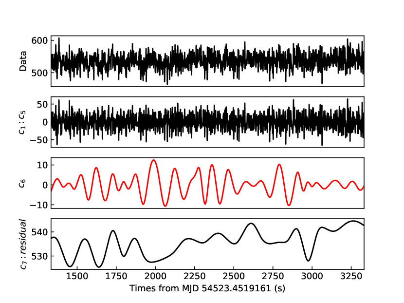
Figure 2: Example of a 1500s light curve, which decomposes to IMFs. (a) The original light curve. (b) The high-frequency noise from the summation of IMF $c_{1}$ to $c_{5}$. (c) The IMF $c_{6}$, which corresponds to $\sim$8 mHz QPOs. (d) The low-frequency noise from the summation of IMF $c_{7}$ to the residual.

The light curve, $x(t)$, may be expressed as the sum of the IMFs, $c_{j}(t)$, and the residual $r_{n}(t)$, $x(t)=\sum_{j=1}^{n}c_{j}(t)+r_{n}(t)$, where n is the number of IMFs. Because the variation time scale of the first IMF component is approximately 3 data points, i.e., 3 $\times$ 1.3333s = 4s, and the variation in the time scale of the second component is twice of the first component (Huang et al., 1998) and so on, the time scale in which we are interested ($\sim$125s) is expected to concentrate at the $6^{th}$ IMF component ($4\times 2^{(6-1)}=128s$). After decomposing the light curve, we determined that the $\sim$8 mHz oscillation can be observed in the sixth IMF, that is, $c_{6}(t)$ as expected (see Figure 2), by confirming the orthogonality of the IMF components (Huang et al., 1998; Hu et al., 2014). We then applied the normalized Hilbert transform (Huang et al., 2009) to obtain the instantaneous phase, frequency and amplitude of IMF $c_{6}(t)$. The instantaneous amplitude $a_{6}(t)$ is defined as the cubic Hermit spline envelope of the local maxima of the absolute values of the IMF $c_{6}(t)$ (Huang et al., 2009). The Hilbert transformation of the normalized IMF $X_{6}(t)=c_{6}(t)/a_{6}(t)$ can be represented as

$$Y_{6}(t)=\frac{1}{\pi}P\int_{-\infty}^{\infty}\frac{X_{6}(t^{\prime})}{t-t^{\prime}}dt^{\prime}$$ (1)

where P is the Cauchy principal value. Thus, we can define an analytical signal $Z_{6}(t)$ and the instantaneous phase function $\theta_{6}(t)$ as

$$Z_{6}(t)=X_{6}(t)+iY_{6}(t)=e^{i\theta_{6}(t)}$$ (2)

Therefore, the instantaneous frequency $\nu_{6}(t)$ can be defined as

$$\nu_{6}(t)=\frac{1}{2\pi}\frac{d\theta_{6}(t)}{dt}$$ (3)

Figure 3 shows Hilbert spectra of $\sim$8 mHz oscillation with more detailed variations in both frequency and amplitude.

To significantly improve detection, the confidence limits can be determined by repeating the CEEMD $10^{3}$ times with different sets of white noise to generate a thousand IMF $c_{6}(t)$, and then the means and standard deviations of the instantaneous amplitude and frequency from these IMF sets can be calculated. Finally, the significant signal is defined by the amplitude above the average of the $3\sigma$ lower limit ($\sim 6$ cts/s) (see Su et al. 2015 for details) that the corresponding data will be selected for further analysis.

3.2 Oscillation profile and phase resolved spectra

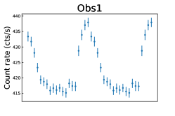
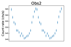
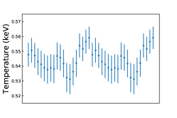
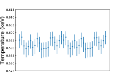
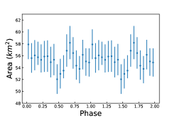
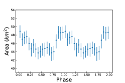
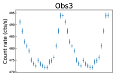
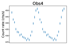
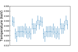
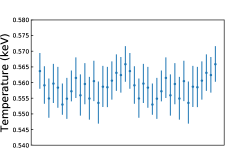
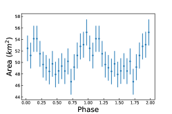
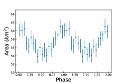
Figure 4: Spectral parameter modulations of neutron-star surface temperature and apparent area. The neutron-star surface temperature is positively correlated with the variation in the neutron-star luminosity for Obs1. The apparent area is also positively correlated with the variation in the neutron-star luminosity for Obs2, Obs3 and Obs4.

After the instantaneous QPO phases $\phi(t)=frac[\theta_{6}(t)]$ are evaluated by HHT (Eq.2), the oscillation profile can be constructed by folding them even though the oscillation period is unstable. The oscillation profiles were constructed by binning the phases into 20 bins per cycle, as shown in Figure 4. The non-sinusoidal nature can be clearly seen in the oscillation profile, that may be approximately described as a fast rise and exponentially decay variation with the rising phase of $\sim$0.3 cycle and the decay phase of $\sim$0.5 cycle.

With the well-defined phase (Eq.2), phase-resolved spectral analysis can be processed. We employed evselect, a standard SAS tool, to extract energy spectra. The spectra were extracted by the selection criteria that PATTERN $<=$ 4 and FLAG $=$ 0. Because the source is very bright, the whole CCD was contaminated by source photons (Lyu et al., 2014, 2015). The background spectra were evaluated by the black hole candidate GX339-4 in quiescence state, that is in the similar sky region and column density along the line of sight (Hiemstra et al., 2011; Sanna et al., 2013).

To obtain the phase-resolved spectra, we divided an oscillation cycle into 20 bins according to the phase defined by HHT, as we did for the oscillation profile, and extracted their individual energy spectra. Using XSPEC v12.10.1, these spectra were fitted with the model (Lyu et al., 2015; Stiele et al., 2016):

$$PHABS\times(BBODYRAD+DISKBB+NTHCOMP)$$

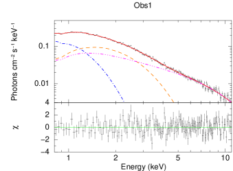
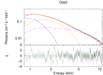
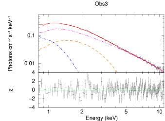
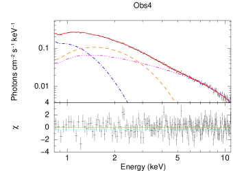
Figure 5: Typical phase resolved spectra from the first phase bin of 4 observations with mHz QPO detections. The blue dash-dotted line, the orange dash line, and purple dash-dotted line represent DISKBB, BBODYRAD, and NTHCOMP, respectively. The red solid line represents the sum of these three components.

where PHABS is photoelectric absorption, BBODYRAD is blackbody from the neutron-star surface, DISKBB (Mitsuda et al., 1984; Makishima et al., 1986) is multi-color disk blackbody to describe the multi-temperature thermal emissions from an accretion disc, and NTHCOMP (Zdziarski et al., 1996; Życki et al., 1999) is inverse Compton scattering process in the corona, with the seed thermal photons coming from the accretion disk (Sanna et al., 2013; Lyu et al., 2014). The interstellar absorption was fixed at $0.36\times 10^{22}cm^{-2}$ (Sanna et al., 2013), selecting the solar abundance from Wilms et al. (2000) and the cross-section from Verner et al. (1996). Because the mHz QPO is considered as metastable nuclear burning on neutron star surface, only the parameters in BBODYRAD were allowed to vary for different phase bins with the parameters of other components being tied to the optimal values evaluated from the detected spectra of the whole cycle. All 20 phase bin spectra of the 4 observations are well fitted by this model, and therefore, the spectral parameter variations on the neutron star surface can be resolved for the whole complete cycle. Figure 5 shows the typical spectra from the first phase bin of 4 observations.

Figure 4 illustrates modulations of the two untied parameters in BBODYRAD, the temperature $T_{bb}$ and the apparent area $R_{\infty}^{2}$, as well as oscillation profile. The apparent area $(R_{\infty}^{2})$ with the mHz QPO phase was calculated by the relation (Sztajno et al., 1985; Stiele et al., 2016):

$$R_{BB}^{2}=R_{\infty}^{2}\times f_{col}^{4}\times\left(1-2\frac{M}{R_{NS}}\right)$$

where G=c=1. The source surface $(R_{BB}^{2})$ was derived from BBODYRAD components with a distance of 6 kpc (Galloway et al., 2006). The factor $(f_{col})$ was set to 1.6 with a helium-enriched environment (Lyu et al., 2015). According to the bolometric flux oscillations that occur during the rise of X-ray burst from Rossi X-ray Timing Explorer (RXTE) observations, $M/R_{NS}$ is 0.126 (Nath et al., 2002).  Table 2 and Table 3 list the untied spectral papameters from BBODYRAD and tied parameters from DISKBB and NTHCOMP, respectively.

Because the count rate is proportional to temperature to the power of 4 and area ($count\ rate\propto L\propto AT^{4}$). We investigated the correlations between the parameters of BBODYRAD and the QPO-profile. Previous studies gave two contradictory results. Stiele et al. (2016) concluded that the area variation dominates the flux oscillation of mHz QPO, whereas Strohmayer et al. (2018) showed that variation is mainly owing to the temperature modulation. To further study which factor is more important to mHz QPO, the Pearson correlation coefficient, r, was applied to investigate the linear relationship between two variables (i.e. count rate vs. area and count rate vs. temperature). The corresponding p-values, under the null hypothesis that two variables follow the Gaussian distribution with zero correlation coefficient, can be used to verify if spectral parameter has strong linear relation to the oscillation count rates. The smaller p-value indicates the stronger correlation between two variables.

Table 4 lists the correlation coefficients and the corresponding p-values. For the Obs1 spectra, there is a strong correlation between $T_{bb}$ and count rates with a linear correlation coefficient r=0.84 and p-value of p=$3\times 10^{-6}$ but almost no correlation between the apparent area and count rates (r=0.19, p=0.41). It indicates that the oscillation is primarily attributed to the temperature variation in an approximately constant apparent area (also refer to Figure 4). For the Obs2 spectra, the marginally positive correlation between $T_{bb}$ and the count rates is r=0.48 (p=0.03), and the apparent area is highly correlated with the count rates with r=0.91 (p=$2\times 10^{-8}$). For the Obs3 and Obs4 spectra, in addition to the marginally positive correlations between $T_{bb}$ and the count rates, where r=0.7 (p=$5\times 10^{-3}$) and r=0.66 (p=$1\times 10^{-3}$) for Obs3 and Obs4, respectively, the apparent area is significantly correlated with the count rates, with r=0.82 (p=$8\times 10^{-6}$) and r=0.88 (p=$2\times 10^{-7}$) for Obs3 and Obs4, respectively. These results show that the area variation dominates the mHz QPO with a constant temperature in Obs 2, 3, and 4 but the temperature variation dominates the mHz QPO with constant area in Obs1. Further implications of these results will be discussed in Section 4.

4 Discussion

We have utilized HHT to characterize the HHT-based timing properties, extracted the 4U 1636-53 $\sim$8 mHz QPOs’ instantaneous phase, and constructed the modulation profiles and phase-resolved spectra for the complete cycle. The mHz QPO is a nonstationary periodic signal, for which the frequency or the amplitude would change with time. Because the dynamic power spectra only obtained the mHz QPO frequency in a time interval, it cannot precisely derive the instantaneous frequency. Conversely, the HHT technique enables us to determine the instantaneous frequency for each data point, that provides an alternative point of view to study the nature of the mHz QPOs. More important is that the HHT may resolve the instantaneous phase, that is believed to be closely related to the physics behind the oscillations rather than the time. With the instantaneous phase, phase-resolved analyses can be processed (e.g. Hu et al., 2014).

In this work, we extracted the instantaneous phase of mHz QPO of 4U 1636-53. Spectral parameter variations can be resolved for the whole mHz oscillation cycle. Our phase-resolved analyses that employ the HHT in this work have a phase resolution of 0.05 cycles for a complete QPO cycle. It shows that HHT has the ability to provide more details in the variations of the spectral parameters. In theoretical model, mHz QPO attributes to the variation of nuclear reaction rate modulations in the hot spot (Heger et al., 2007) that may cause the temperature oscillation or apparent area variation. Recently, there are two contradictory results for mHz QPO observations. Strohmayer et al. (2018) revealed significant oscillations at the frequency $\sim$8 mHz in GS 1826-238 from the Neutron Star Interior Composition Explorer (NICER) observation on September 9, 2017. This $\sim$8 mHz frequency and its amplitude are consistent with other accreting neutron star systems with mHz QPO detections. Their phase-resolved spectra show that the mHz oscillation is produced by modulation of the temperature component of blackbody emission from the neutron star surface with a constant emission area through the oscillation cycle. However, Stiele et al. (2016) provided a different conclusion for the mHz QPO of 4U1636-53. Their phase-resolved spectra showed that mHz QPOs are owing to the periodically changing size of the hot spot with a constant temperature. In this work, the detailed and more precise phase resolved spectra can exhibit the correlations shown in Section 3.2. The result reveals that the area variation dominates the mHz QPO in Obs 2, 3 and 4, but temperature variation has much stronger correlation with the oscillation count rate than the apparent area in Obs1. This indicates that either temperature or apparent area variations of the hot spot may dominate the mHz QPO oscillation. The cause of the difference is not clear but it might be related to the spectral state of the source. Figure 1 in Lyu et al. (2015) showed the spectral states of these 4 observations in the color-color diagram. We find that the hard color of Obs1 is higher than the others. This is a possible clue why the Obs1 behaves differently than the other three. However, because there are only 4 observations with mHz QPO detections, more observations are required to verify if the different behavior of Obs1 is due to the spectral state or just a coincident.

One of the important factors in marginally stable burning is the accretion rate. The theoretical interpretation showed that the accretion rate is close to the Eddington accretion rate ($\sim\dot{M}_{Edd}$) (Heger et al., 2007), but current observations indicated that the accretion rate is much lower ($\sim 0.1\dot{M}_{Edd}$) for the sources with mHz QPOs. Fujimoto et al. (1981) suggested that the burst ignition of neutron star depends on the accretion rate per unit area, $\dot{m}$ instead of the overall accretion rate. The local accretion rate ($\dot{m}$) does not need to be the same everywhere on the neutron star surface (Bildsten, 1998). The nuclear burning depends on the local accretion rate (Bildsten, 1998; Heger et al., 2007). For a fast-spinning neutron star, a latitude change in the local accretion rate is influenced by the variation in the effective surface gravity from the equator to the pole (Strohmayer et al., 2018). Lyu et al. (2016) discovered that mHz QPOs only associate with bursts with positive convexity. Because Maurer & Watts (2008) found that type-I X-ray bursts that ignite at the equator always have positive convexity, the mHz QPO locates on the equator of the neutron star. Strohmayer et al. (2018) roughly estimate the effective surface gravity of the neutron star in 4U1636-53; the value on the pole can be $\sim 11\%$ stronger than the one on the equator. They found this value is sufficient for influencing marginally stable burning by effecting the local accretion rate, and marginally stable burning on the equator belt on the neutron star surface is possible (Altamirano et al., 2008; Strohmayer et al., 2018). Even though using the local accretion rate can explain marginally stable nuclear burning, a more complete theoretical model is required to explain the phenomena that we observed. Heger et al. (2007) calculated that marginally stable burning is one-dimensional; thus, the burning area is not explored (Strohmayer et al., 2018).

Data collected by XMM-Newton were analyzed in this work. The mHz QPOs are typically detected in low energy bands (1-5 keV); thus, the energy range of XMM-Newton (0.1 to 15 keV) is beneficial for observing the mHz QPOs. XMM-Newton is a high altitude satellite with an orbital period of 2789.6 minutes, that enables it to observe a source for a long time without interruption. Because HHT prefers continuous data, the data collected by XMM-Newton are beneficial for using the HHT to analyze mHz QPOs. The high spectrum resolution of XMM-Newton is also advantageous to the spectral analysis. In addition to XMM-Newton, Nuclear Spectroscopic Telescope Array mission (NuSTAR) and NICER are possible choices that can be used to study mHz QPOs. Unfortunately, because NuSTAR focuses on high X-ray energy bands (3-79 keV), it may not be suitable for studying mHz QPOs (typically detected in lower energy bands). The time resolution of NICER is 100 nsec, and its spectral band overlaps RXTE and XMM-Newton (0.2-12 keV). The high time resolution enables us to analyze more timing properties by the HHT. NICER has a large effective area, that is beneficial for collecting photons. More photons have more timing information; thus, NICER would be a reasonable choice to perform timing analysis. However, NICER is a facility on-board the International Space Station (ISS), and the observations are usually interrupted due to Earth occultation for each ISS orbital cycle ($\sim 90$ min). On the other hand, X-ray telescopes that are expected to be operated in the next decade, such as enhanced X-ray Timing and Polarimetry mission (eXTP) and X-ray Imaging and Spectroscopy Mission (XRISM), although they have better time and spectral resolution in the low energy band ($\sim 0.5-10$ keV), the Earth occultation would induce too much alias in the HHT analysis for these low-altitude satellites, similar to NICER. These make the data collected by XMM-Newton the best data for analysis by the HHT for the mHz QPO investigations. In the future, more XMM-Newton observations will enable us to investigate the physical reasons of mHz QPOs by using the HHT to analyze more timing properties and spectral modulation of mHz QPOs.

Table 1: XMM-Newton observations of 4U1636-53 from 2000 to 2015.

Observation ID	Observation date	PN exposure time	Time span of QPO	Note
		(seconds)	(seconds)
0105470101	2000-09-07	23607	No detection	-
0105470401	2001-08-24	21601	No detection	-
0303250201	2005-08-29	31336	No detection	-
0500350301	2007-09-28	31935	5420	Obs1
0500350401	2008-02-27	39942	16340	Obs2
0606070101	2009-03-14	41179	13317	Obs3
0606070201	2009-03-25	28939	No detection	-
0606070301	2009-09-05	43200	11949	Obs4
0606070401	2009-09-11	27239	No detection	-
0764180201	2015-08-25	40800	No detection	-
0764180301	2015-09-05	36899	No detection	-
0764180401	2015-09-18	37100	No detection	-

Table 2: All BBODYRAD parameters in this work.

Note	Phase	Temperature (keV)	Area normalized	$\chi^{2}/d.o.f$	Note	Phase	Temperature (keV)	Area normalized	$\chi^{2}/d.o.f$
Obs1	1	$0.5477_{-0.0080}^{+0.0080}$	$789_{-34}^{+35}$	$138.46/155$	Obs2	1	$0.5952_{-0.0053}^{+0.0038}$	$665_{-22}^{+19}$	$173.10/169$
Obs1	2	$0.5507_{-0.0083}^{+0.0083}$	$757_{-34}^{+34}$	$155.41/159$	Obs2	2	$0.5971_{-0.0052}^{+0.0038}$	$639_{-21}^{+19}$	$165.19/170$
Obs1	3	$0.5472_{-0.0084}^{+0.0085}$	$764_{-34}^{+35}$	$128.89/156$	Obs2	3	$0.5913_{-0.0055}^{+0.0039}$	$644_{-22}^{+19}$	$185.82/171$
Obs1	4	$0.5430_{-0.0090}^{+0.0090}$	$767_{-18}^{+36}$	$155.12/156$	Obs2	4	$0.5895_{-0.0056}^{+0.0040}$	$647_{-22}^{+19}$	$154.66/171$
Obs1	5	$0.5412_{-0.0091}^{+0.0091}$	$756_{-29}^{+36}$	$172.28/157$	Obs2	5	$0.5909_{-0.0057}^{+0.0040}$	$625_{-22}^{+19}$	$210.04/170$
Obs1	6	$0.5390_{-0.0092}^{+0.0092}$	$761_{-35}^{+36}$	$119.45/159$	Obs2	6	$0.5948_{-0.0052}^{+0.0040}$	$606_{-25}^{+19}$	$199.24/170$
Obs1	7	$0.5377_{-0.0095}^{+0.0094}$	$762_{-36}^{+36}$	$149.83/159$	Obs2	7	$0.5904_{-0.0057}^{+0.0040}$	$618_{-26}^{+19}$	$160.11/171$
Obs1	8	$0.5387_{-0.0093}^{+0.0092}$	$748_{-35}^{+35}$	$148.07/157$	Obs2	8	$0.5917_{-0.0058}^{+0.0040}$	$604_{-26}^{+19}$	$121.97/171$
Obs1	9	$0.5381_{-0.0095}^{+0.0095}$	$754_{-36}^{+36}$	$134.25/159$	Obs2	9	$0.5960_{-0.0056}^{+0.0040}$	$594_{-21}^{+19}$	$166.33/171$
Obs1	10	$0.5468_{-0.0091}^{+0.0091}$	$709_{-33}^{+34}$	$157.38/158$	Obs2	10	$0.5932_{-0.0058}^{+0.0040}$	$599_{-19}^{+19}$	$166.44/177$
Obs1	11	$0.5458_{-0.0089}^{+0.0089}$	$721_{-34}^{+34}$	$178.75/157$	Obs2	11	$0.5893_{-0.0059}^{+0.0041}$	$606_{-21}^{+19}$	$157.21/172$
Obs1	12	$0.5418_{-0.0093}^{+0.0093}$	$737_{-18}^{+35}$	$143.77/158$	Obs2	12	$0.5896_{-0.0058}^{+0.0040}$	$606_{-26}^{+19}$	$185.17/172$
Obs1	13	$0.5323_{-0.0099}^{+0.0099}$	$774_{-37}^{+38}$	$141.56/157$	Obs2	13	$0.5897_{-0.0058}^{+0.0040}$	$612_{-21}^{+19}$	$154.24/172$
Obs1	14	$0.5312_{-0.0101}^{+0.0100}$	$793_{-37}^{+39}$	$170.59/157$	Obs2	14	$0.5903_{-0.0059}^{+0.0041}$	$607_{-21}^{+19}$	$161.58/171$
Obs1	15	$0.5363_{-0.0093}^{+0.0093}$	$769_{-36}^{+36}$	$138.23/156$	Obs2	15	$0.5965_{-0.0051}^{+0.0039}$	$592_{-26}^{+19}$	$178.58/172$
Obs1	16	$0.5420_{-0.0091}^{+0.0090}$	$741_{-32}^{+35}$	$135.26/158$	Obs2	16	$0.5967_{-0.0056}^{+0.0040}$	$596_{-26}^{+19}$	$181.53/170$
Obs1	17	$0.5538_{-0.0082}^{+0.0082}$	$731_{-33}^{+30}$	$154.51/157$	Obs2	17	$0.5937_{-0.0050}^{+0.0039}$	$633_{-27}^{+19}$	$196.67/170$
Obs1	18	$0.5516_{-0.0081}^{+0.0082}$	$765_{-33}^{+34}$	$171.72/156$	Obs2	18	$0.5914_{-0.0053}^{+0.0041}$	$662_{-22}^{+19}$	$184.78/171$
Obs1	19	$0.5565_{-0.0081}^{+0.0080}$	$748_{-33}^{+30}$	$149.87/157$	Obs2	19	$0.5948_{-0.0048}^{+0.0037}$	$658_{-25}^{+19}$	$192.30/171$
Obs1	20	$0.5591_{-0.0075}^{+0.0076}$	$747_{-32}^{+32}$	$160.29/156$	Obs2	20	$0.5975_{-0.0050}^{+0.0036}$	$661_{-22}^{+19}$	$202.71/171$
Obs3	1	$0.5398_{-0.0047}^{+0.0048}$	$714_{-30}^{+30}$	$180.53/171$	Obs4	1	$0.5637_{-0.0056}^{+0.0058}$	$820_{-20}^{+23}$	$154.50/169$
Obs3	2	$0.5388_{-0.0048}^{+0.0049}$	$697_{-31}^{+30}$	$189.44/170$	Obs4	2	$0.5591_{-0.0059}^{+0.0061}$	$818_{-23}^{+23}$	$190.83/169$
Obs3	3	$0.5270_{-0.0051}^{+0.0052}$	$737_{-31}^{+31}$	$224.64/170$	Obs4	3	$0.5549_{-0.0062}^{+0.0063}$	$825_{-24}^{+24}$	$177.72/169$
Obs3	4	$0.5240_{-0.0053}^{+0.0055}$	$737_{-31}^{+31}$	$188.45/171$	Obs4	4	$0.5597_{-0.0062}^{+0.0063}$	$776_{-23}^{+23}$	$184.26/170$
Obs3	5	$0.5292_{-0.0052}^{+0.0054}$	$701_{-31}^{+30}$	$155.28/171$	Obs4	5	$0.5584_{-0.0064}^{+0.0066}$	$767_{-23}^{+23}$	$156.55/169$
Obs3	6	$0.5289_{-0.0055}^{+0.0056}$	$676_{-31}^{+30}$	$180.79/170$	Obs4	6	$0.5530_{-0.0033}^{+0.0067}$	$796_{-23}^{+24}$	$193.24/170$
Obs3	7	$0.5291_{-0.0055}^{+0.0057}$	$668_{-31}^{+30}$	$150.00/170$	Obs4	7	$0.5549_{-0.0064}^{+0.0066}$	$777_{-23}^{+23}$	$201.52/170$
Obs3	8	$0.5293_{-0.0055}^{+0.0057}$	$659_{-31}^{+30}$	$199.10/170$	Obs4	8	$0.5572_{-0.0032}^{+0.0066}$	$767_{-23}^{+23}$	$123.72/170$
Obs3	9	$0.5288_{-0.0054}^{+0.0056}$	$677_{-31}^{+30}$	$189.07/171$	Obs4	9	$0.5615_{-0.0064}^{+0.0066}$	$734_{-22}^{+23}$	$161.16/170$
Obs3	10	$0.5317_{-0.0055}^{+0.0057}$	$652_{-30}^{+30}$	$146.95/171$	Obs4	10	$0.5559_{-0.0064}^{+0.0067}$	$763_{-23}^{+23}$	$153.28/168$
Obs3	11	$0.5287_{-0.0058}^{+0.0059}$	$661_{-31}^{+30}$	$180.95/171$	Obs4	11	$0.5595_{-0.0064}^{+0.0066}$	$740_{-23}^{+23}$	$170.36/170$
Obs3	12	$0.5271_{-0.0055}^{+0.0056}$	$672_{-31}^{+30}$	$176.76/170$	Obs4	12	$0.5549_{-0.0067}^{+0.0069}$	$754_{-23}^{+24}$	$207.85/168$
Obs3	13	$0.5287_{-0.0056}^{+0.0058}$	$660_{-31}^{+30}$	$189.05/171$	Obs4	13	$0.5605_{-0.0064}^{+0.0065}$	$737_{-23}^{+23}$	$165.73/170$
Obs3	14	$0.5268_{-0.0056}^{+0.0058}$	$683_{-31}^{+31}$	$208.90/172$	Obs4	14	$0.5535_{-0.0066}^{+0.0068}$	$767_{-23}^{+24}$	$174.87/172$
Obs3	15	$0.5368_{-0.0055}^{+0.0056}$	$635_{-31}^{+30}$	$179.65/171$	Obs4	15	$0.5587_{-0.0064}^{+0.0066}$	$755_{-23}^{+23}$	$168.19/168$
Obs3	16	$0.5322_{-0.0054}^{+0.0055}$	$670_{-31}^{+31}$	$141.18/172$	Obs4	16	$0.5585_{-0.0063}^{+0.0065}$	$778_{-12}^{+23}$	$145.32/169$
Obs3	17	$0.5322_{-0.0052}^{+0.0053}$	$697_{-31}^{+31}$	$202.26/172$	Obs4	17	$0.5606_{-0.0060}^{+0.0061}$	$792_{-23}^{+24}$	$200.99/168$
Obs3	18	$0.5351_{-0.0049}^{+0.0050}$	$719_{-31}^{+31}$	$170.80/171$	Obs4	18	$0.5631_{-0.0057}^{+0.0059}$	$800_{-20}^{+12}$	$163.63/170$
Obs3	19	$0.5407_{-0.0047}^{+0.0048}$	$723_{-31}^{+30}$	$173.93/171$	Obs4	19	$0.5624_{-0.0056}^{+0.0057}$	$831_{-23}^{+23}$	$203.28/169$
Obs3	20	$0.5360_{-0.0047}^{+0.0048}$	$752_{-31}^{+31}$	$173.03/171$	Obs4	20	$0.5659_{-0.0056}^{+0.0058}$	$814_{-23}^{+21}$	$158.42/170$

Table 3: Spectral parameters of DISKBB and NTHCOMP.

Component	Parameter	Obs1	Obs2	Obs3	Obs4
DISKBB	$\kappa T_{0}$ (keV)	$0.277_{-0.007}^{+0.007}$	$0.275_{-0.005}^{+0.005}$	$0.233_{-0.007}^{+0.007}$	$0.287_{-0.006}^{+0.006}$
	$Nor$	$9441_{-738}^{+842}$	$10125_{-526}^{+576}$	$16454_{-1550}^{+1765}$	$8126_{-514}^{+551}$
NTHCOMP	$NTHCOMP(\Gamma)$	$1.483_{-0.057}^{+0.054}$	$1.549_{-0.026}^{+0.025}$	$1.727_{-0.024}^{+0.021}$	$1.484_{-0.039}^{+0.036}$
	$kT_{e}(keV)$	$2.196_{-0.071}^{+0.076}$	$2.334_{-0.037}^{+0.039}$	$2.751_{-0.071}^{+0.073}$	$2.215_{-0.047}^{+0.049}$
	$Nor$	$0.113_{-0.019}^{+0.020}$	$0.198_{-0.016}^{+0.017}$	$0.318_{-0.023}^{+0.023}$	$0.134_{-0.016}^{+0.017}$
$\chi^{2}/d.o.f$		3100.6/3144	3874.6/3638	3729.8/3417	3546.7/3387

Table 4: The correlation between count rate and temperature (T) and between count rate and area (A).

Note	T:r-value	T:p-value	A:r-value	A:p-value
Obs1	0.84	$3\times 10^{-6}$	0.19	0.41
Obs2	0.48	0.03	0.91	$2\times 10^{-8}$
Obs3	0.70	0.005	0.82	$8\times 10^{-6}$
Obs4	0.66	0.001	0.88	$2\times 10^{-7}$

Figure 1: Dynamic power spectra of the 4 observations with significant detections of mHz QPO. The frequency of mHz QPO drifts from $\sim$10 to 8 mHz as it approaches the type-I burst, and the variation in oscillation power can be clearly seen.

Figure 3: Hilbert spectra of mHz QPOs. The color on the z-axis represents the amplitude. Some instantaneous frequency drift above 15 mHz, but their amplitudes are less 3$\sigma$ significance ($\sim$6 cts/s). These data were neglected when we applied the confidence limits. The contour is the dynamic Lomb-Scargle periodogram of the detrended light curve.

References

- Altamirano et al. (2008) Altamirano, D., van der Klis, M., Wijnands, R., & Cumming, A. 2008, ApJ, 673, L35
- Arnaud (1996) Arnaud, K. A. 1996, Astronomical Society of the Pacific Conference Series, Vol. 101, XSPEC: The First Ten Years, ed. G. H. Jacoby & J. Barnes, 17
- Astropy Collaboration et al. (2013) Astropy Collaboration, Robitaille, T. P., Tollerud, E. J., et al. 2013, A&A, 558, A33
- Bildsten (1998) Bildsten, L. 1998, in NATO Advanced Science Institutes (ASI) Series C, Vol. 515, NATO Advanced Science Institutes (ASI) Series C, ed. R. Buccheri, J. van Paradijs, & A. Alpar, 419
- Cooper & Narayan (2007) Cooper, R. L., & Narayan, R. 2007, The Astrophysical Journal, 657, L29
- Fujimoto et al. (1981) Fujimoto, M. Y., Hanawa, T., & Miyaji, S. 1981, ApJ, 247, 267
- Gabriel (2017) Gabriel, C. 2017, in The X-ray Universe 2017, ed. J.-U. Ness & S. Migliari, 84
- Galloway & Keek (2017) Galloway, D. K., & Keek, L. 2017, arXiv e-prints, arXiv:1712.06227
- Galloway et al. (2006) Galloway, D. K., Psaltis, D., Muno, M. P., & Chakrabarty, D. 2006, ApJ, 639, 1033
- Heger et al. (2007) Heger, A., Cumming, A., & Woosley, S. E. 2007, ApJ, 665, 1311
- Hiemstra et al. (2011) Hiemstra, B., Méndez, M., Done, C., et al. 2011, MNRAS, 411, 137
- Hu et al. (2014) Hu, C.-P., Chou, Y., Yang, T.-C., & Su, Y.-H. 2014, ApJ, 788, 31
- Huang et al. (2009) Huang, N., Wu, Z., Long, S., et al. 2009, Advances in Adaptive Data Analysis, 1, 177
- Huang & Wu (2008) Huang, N. E., & Wu, Z. 2008, Reviews of Geophysics, 46, RG2006
- Huang et al. (1998) Huang, N. E., Shen, Z., Long, S. R., et al. 1998, Proceedings of the Royal Society of London Series A, 454, 903
- Keek et al. (2014) Keek, L., Cyburt, R. H., & Heger, A. 2014, ApJ, 787, 101
- Keek & Heger (2015) Keek, L., & Heger, A. 2015, Monthly Notices of the Royal Astronomical Society: Letters, 456, L11
- Keek et al. (2009) Keek, L., Langer, N., & in’t Zand, J. J. M. 2009, A&A, 502, 871
- Linares et al. (2012) Linares, M., Altamirano, D., Chakrabarty, D., Cumming, A., & Keek, L. 2012, The Astrophysical Journal, 748, 82
- Lyu et al. (2014) Lyu, M., Méndez, M., & Altamirano, D. 2014, MNRAS, 445, 3659
- Lyu et al. (2016) Lyu, M., Méndez, M., Altamirano, D., & Zhang, G. 2016, MNRAS, 463, 2358
- Lyu et al. (2015) Lyu, M., Méndez, M., Zhang, G., & Keek, L. 2015, MNRAS, 454, 541
- Makishima et al. (1986) Makishima, K., Maejima, Y., Mitsuda, K., et al. 1986, ApJ, 308, 635
- Maurer & Watts (2008) Maurer, I., & Watts, A. L. 2008, MNRAS, 383, 387
- Mitsuda et al. (1984) Mitsuda, K., Inoue, H., Koyama, K., et al. 1984, PASJ, 36, 741
- Nath et al. (2002) Nath, N. R., Strohmayer, T. E., & Swank, J. H. 2002, ApJ, 564, 353
- Revnivtsev et al. (2001) Revnivtsev, M., Churazov, E., Gilfanov, M., & Sunyaev, R. 2001, A&A, 372, 138
- Sanna et al. (2013) Sanna, A., Hiemstra, B., Méndez, M., et al. 2013, MNRAS, 432, 1144
- Scargle (1982) Scargle, J. D. 1982, ApJ, 263, 835
- Stiele et al. (2016) Stiele, H., Yu, W., & Kong, A. K. H. 2016, ApJ, 831, 34
- Strohmayer & Altamirano (2012) Strohmayer, T. E., & Altamirano, D. 2012, in American Astronomical Society Meeting Abstracts, Vol. 219, American Astronomical Society Meeting Abstracts #219, 249.03
- Strohmayer et al. (2018) Strohmayer, T. E., Gendreau, K. C., Altamirano, D., et al. 2018, ApJ, 865, 63
- Su et al. (2015) Su, Y.-H., Chou, Y., Hu, C.-P., & Yang, T.-C. 2015, ApJ, 815, 74
- Sztajno et al. (1985) Sztajno, M., van Paradijs, J., Lewin, W. H. G., et al. 1985, ApJ, 299, 487
- van der Klis (2006) van der Klis, M. 2006, Rapid X-ray Variability, ed. W. H. G. Lewin & M. van der Klis, 39–112
- Verner et al. (1996) Verner, D. A., Ferland, G. J., Korista, K. T., & Yakovlev, D. G. 1996, ApJ, 465, 487
- Wang et al. (2014) Wang, Y.-H., Yeh, C.-H., Young, H.-W. V., Hu, K., & Lo, M.-T. 2014, Physica A Statistical Mechanics and its Applications, 400, 159
- Wilms et al. (2000) Wilms, J., Allen, A., & McCray, R. 2000, ApJ, 542, 914
- Yeh et al. (2010) Yeh, J.-R., Shieh, J.-S., & Huang, N. 2010, Advances in Adaptive Data Analysis, 2, 135
- Yu & van der Klis (2002) Yu, W., & van der Klis, M. 2002, The Astrophysical Journal, 567, L67
- Zdziarski et al. (1996) Zdziarski, A. A., Johnson, W. N., & Magdziarz, P. 1996, MNRAS, 283, 193
- Życki et al. (1999) Życki, P. T., Done, C., & Smith, D. A. 1999, MNRAS, 309, 561