Eigenstate thermalization hypothesis and eigenstate-to-eigenstate fluctuations

Abstract

We investigate the extent to which the eigenstate thermalization hypothesis (ETH) is valid or violated in the nonintegrable and the integrable spin-$1/2$ XXZ chains. We perform the energy-resolved analysis of statistical properties of matrix elements of observables in the energy eigenstate basis. The Hilbert space is divided into energy shells of constant width, and a block submatrix is constructed whose columns and rows correspond to the eigenstates in the respective energy shells. In each submatrix, we measure the second moment of off-diagonal elements in a column. The columnar second moments are distributed with a finite variance for finite-sized systems. We show that the relative variance of the columnar second moments decreases as the system size increases in the nonintegrable system. The self-averaging behavior indicates that the energy eigenstates are statistically equivalent to each other, which is consistent with the ETH. In contrast, the relative variance does not decrease with the system size in the integrable system. The persisting eigenstate-to-eigenstate fluctuation implies that the matrix elements cannot be characterized with the energy parameters only. Our result explains the origin for the breakdown of the fluctuation dissipation theorem in the integrable system. The eigenstate-to-eigenstate fluctuations sheds a new light on the meaning of the ETH.

I Introduction

Since the birth of quantum mechanics, it has been a fascinating question to ask whether an isolated quantum system can approach the thermal equilibrium state through the unitary time evolution [1, 2]. The thermalization requires that the Hamiltonian eigenstate expectation value of an observable should be equal to the equilibrium ensemble average and that temporal fluctuations and responses should be governed by the fluctuation dissipation theorem (FDT). It is believed that the eigenstate thermalization hypothesis (ETH) provides a mechanism for the quantum thermalization [3, 4, 5, 6].

An isolated quantum system is characterized by the Hamiltonian $\hat{H}$. Let $\{\ket{\alpha}\}$ and $\{E_{\alpha}\}$ be the energy eigenstates and the eigenvalues, respectively. The ETH [3, 7] proposes that matrix elements $O_{\gamma\alpha}\equiv\bra{\gamma}\hat{O}\ket{\alpha}$ of an observable $\hat{O}$ should take the form of

$$O_{\gamma\alpha}=O(E_{\gamma\alpha})\delta_{\gamma\alpha}+e^{-S(E_{\gamma\alpha})/2}f_{O}(E_{\gamma\alpha},\omega_{\gamma\alpha})R_{\gamma\alpha},$$ (1)

where $E_{\gamma\alpha}\equiv(E_{\gamma}+E_{\alpha})/2$, $\omega_{\gamma\alpha}\equiv E_{\gamma}-E_{\alpha}$, $S(E)$ is the thermodynamic entropy with the Boltzmann constant $k_{B}=1$, $R_{\gamma\alpha}$’s are elements of a random matrix in the Gaussian orthogonal or unitary ensemble, and $O$ and $f_{O}$ are smooth functions of their arguments.

According to the ETH, a diagonal element, eigenstate expectation value, is given by

$$O_{\alpha\alpha}=O(E_{\alpha})+e^{-S(E_{\alpha})/2}f_{O}(E_{\alpha},0)R_{\alpha\alpha}.$$ (2)

Since the entropy is an extensive quantity, the second term decreases exponentially with the system size. Thus, the diagonal elements follow the Gaussian distribution whose variance is exponentially small. The ETH for off-diagonal elements reads as

$$O_{\gamma\alpha(\neq\gamma)}=e^{-S(E_{\gamma\alpha})/2}f_{O}(E_{\gamma\alpha},\omega_{\gamma\alpha})R_{\gamma\alpha}.$$ (3)

The off-diagonal elements govern temporal fluctuations. The ETH guarantees that an isolated quantum system in an energy eigenstate obeys the FDT [7, 8, 5, 9, 10].

The ETH ansatz has been tested extensively for the generic nonintegrable and the integrable systems [11, 12, 13, 14, 15, 16, 17, 18, 19, 20, 21, 22, 23, 24, 25, 26, 27, 10]. The former is known to obey the ETH, while the latter does not obey the ETH . We present a brief review on the previous numerical works on the ETH.

For the diagonal elements, one may measure the difference $\delta O_{\alpha}=|O_{(\alpha+1)(\alpha+1)}-O_{\alpha\alpha}|$ in the eigenstate expectation values of neighboring eigenstates [16]. In the nonintegrable systems, both their support and the mean value have been shown to decrease exponentially with the system size [16, 20, 23, 25]. These behaviors are consistent with Eq. (2). On the other hand, in the integral systems, they have a nonvanishing support and their mean value decreases algebraically or more slowly with the system size [18, 25].

The off-diagonal elements have been shown to follow the Gaussian distribution in the nonintegrable systems. The variance is inversely proportional to the density of states and decreases exponentially with the system size [25, 27]. These behaviors are also consistent with the ETH prediction. Using the variance and the density of states, one can estimate the function $|f_{O}(E,\omega)|$ numerically [20].

The off-diagonal elements have been also investigated in the integrable systems. They do not follow the Gaussian distribution [17, 25]. A model study [25] reports that they may follow a log-normal distribution. Interestingly, the variance is also found to be inversely proportional to the density of states as in the nonintegrable systems [29, 25, 26].

The off-diagonal elements in the nonintegrable and the integrable systems share two important features: (i) The variance is inversely proportional to the density of states, and (ii) it seems to be a smooth function of $E_{\gamma\alpha}$ and $\omega_{\gamma\alpha}$. These suggest that the off-diagonal elements in the integrable systems may follow the ansatz of Eq. (3) with non-Gaussian random variables $R_{\gamma\alpha}$. We notice that the two common features are the essential ingredients leading to the FDT at the energy eigenstates [5, 9]. Apparently, it is contradictory to the known fact that the FDT is violated in the integrable systems [30, 31].

In this paper, we perform the energy-resolved study of the statistical properties of matrix elements $\{O_{\gamma\alpha}\}$ of observables in the integrable and in the nonintegrable spin-1/2 XXZ models. From the full matrix, one can construct a block submatrix $\tilde{O}$ whose columns and rows correspond to the energy eigenstates belonging to an energy shell of width $\Delta_{E}$. Each block is characterized with constant energy parameters $E_{\gamma\alpha}$ and $\omega_{\gamma\alpha}$ up to $\Delta_{E}$. Investigating the probability distribution of the elements within each block, one can test the ETH ansatz at various energy values. Furthermore, one can also investigate an eigenstate-to-eigenstate fluctuation by comparing the probability distributions of matrix elements in different columns.

As a main result, we will show that the eigenstate-to-eigenstate fluctuation vanishes in the nonintegrable system while it remains finite in the integrable system in the large system size limit. The ETH ansatz in Eq. (3) for the off-diagonal elements requires that all matrix elements should be equivalent statistically within a block submatrix for a sufficiently small $\Delta_{E}$. Otherwise, the function $f_{O}(E,\omega)$ cannot be a smooth function of the arguments. The eigenstate-to-eigenstate fluctuation disproves the existence of such a smooth function in the integrable system. Thus, it resolves the puzzle in regard to the FDT.

This paper is organized as follows. In Sec. II, we introduce the spin-1/2 XXZ Hamiltonian and the observables investigated in this paper. We also explain the method to construct block submatrices. In Sec. III, we present the numerical results for the energy-resolved statistics for matrix elements within each submatrix. In Sec. IV, we investigate the eigenstate-to-eigenstate fluctuations in statistics of off-diagonal matrix elements. It will uncover the clear difference between the integrable system and the nonintegrable system. We conclude the paper with summary and discussions in Sec. V.

II Model system and numerical setup

We study the spin-1/2 XXZ model in a one-dimensional lattice of $L$ sites under the periodic boundary condition. Let $\hat{\sigma}_{l}^{p}$ be the Pauli matrix in the $p~{}(=x,y,z)$ direction at site $l~{}(=1,\cdots,L)$. The XXZ Hamiltonian is given by

$$\hat{H}=\frac{1}{1+\lambda}\sum_{l=1}^{L}\left[\hat{h}_{l,l+1}+\lambda\hat{h}_{l,l+2}\right],$$ (4)

where $\hat{h}_{l,m}\equiv-\frac{J}{2}(\hat{\sigma}_{l}^{x}\hat{\sigma}_{m}^{x}+\hat{\sigma}_{l}^{y}\hat{\sigma}_{m}^{y}+\Delta\hat{\sigma}_{l}^{z}\hat{\sigma}_{m}^{z})$. Note that $\Delta$ is an anisotropy parameter and $\lambda$ is the relative strength of the next nearest neighbor interactions. The overall coupling constant $J$ will be set to unity so that the energy becomes dimensionless. The Hamiltonian is integrable when $\lambda=0$, and nonintegrable when $\lambda\neq 0$ [21, 24, 9].

The Hamiltonian commutes with the total magnetization operator in the $z$ direction, the translation operator, the spatial reflection operator, and the spin inversion operator. Especially, in the translationally invariant subspace with zero magnetization, all the symmetry operators mutually commute [25, 32]. We focus our attention on the translationally invariant subspace with zero magnetization that are even under the spatial reflection and the spin inversion, which will be called the maximum symmetry sector (MSS) [32]. The Hilbert space dimensions of the MSS are $D=2518,8359$, and $28968$ for $L=20,22$, and $24$, respectively. In this paper, we present the numerical results obtained at $\lambda=0$ (integrable case) and $\lambda=1$ (nonintegrable case) with fixed $\Delta=1/2$.

We numerically diagonalize the Hamiltonian in the MSS to obtain the energy eigenvalues $\{E_{\alpha}\}$ and the eigenstates $\{\ket{\alpha}\}$ with $\alpha=1,\cdots,D$ [32, 33]. The eigenstates are arranged in the ascending order of the energy eigenvalues. Using the eigenvalue spectrum, we define a function

$$\bar{E}(\beta)=\frac{\sum_{\gamma}E_{\gamma}e^{-\beta E_{\gamma}}}{\sum_{\gamma}e^{-\beta E_{\gamma}}}.$$ (5)

If the system is thermal, $\bar{E}(\beta)$ corresponds to the equilibrium canonical ensemble average of the energy at the inverse temperature $\beta$. One can assign the temperature to each energy eigenstate using the relation $\bar{E}(\beta)=E_{\alpha}$. Such an assignment is useful even in the nonthermal case since it allows one to parametrize the energy eigenvalue with an intensive variable $\beta$. The parameter $\beta$ will be called the inverse temperature in both cases for convenience.

Once all eigenvectors are obtained, it is straightforward to calculate the matrix elements $O_{\gamma\alpha}$ of an observable $\hat{O}$. For a detailed study, we introduce a block submatrix. To a given value of $\beta$ and $\bar{E}=\bar{E}(\beta)$, we define an energy shell $\mathcal{S}_{a}$ ($a=0,\pm 1,\pm 2,\cdots$) as the subspace consisting of energy eigenstates with $\bar{E}+(a-\frac{1}{2})\Delta_{E}\leq E_{\alpha}<\bar{E}+(a+\frac{1}{2})\Delta_{E}$. The energy resolution $\Delta_{E}$ is taken to be a constant independent of $L$. The number of energy eigenstates within a shell $\mathcal{S}_{a}$ is denoted by $\mathcal{N}_{a}$. A block submatrix $\tilde{O}^{(b,a)}(\beta)$ is defined as a $(\mathcal{N}_{b}\times\mathcal{N}_{a})$ matrix consisting of elements $O_{\gamma\alpha}$ with $\ket{\gamma}\in\mathcal{S}_{b}$ and $\ket{\alpha}\in\mathcal{S}_{a}$. All elements of $\tilde{O}^{(b,a)}$ are characterized by constant $E_{\gamma\alpha}\simeq\bar{E}(\beta)+(a+b)\Delta_{E}/2$ and $\omega_{\gamma\alpha}\simeq(b-a)\Delta_{E}$ up to $\Delta_{E}$. We illustrate the block submatrix structure in Fig. 1.

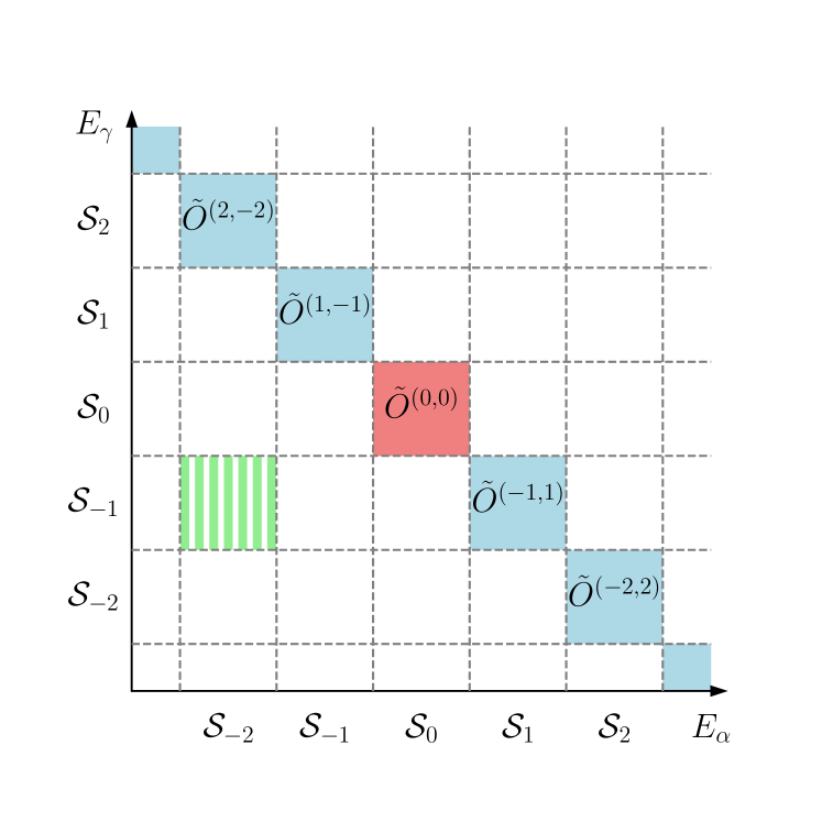
Figure 1: Illustration of the block submatrix structure. Each square corresponds to a block submatrix. In Sec. III, we study the statistical properties of matrix elements in each shaded block. The columnar stripe represents matrix elements involving a given energy eigenstate. Statistical fluctuations from column to column, that is, the eigenstate-to-eigenstate fluctuations will be studied in Sec. IV.

As observables, we choose the nearest neighbor interaction energy

$$\hat{O}_{1}=\frac{1}{\sqrt{L}}\sum_{l}\hat{\sigma}_{l}^{z}\hat{\sigma}_{l+1}^{z}$$ (6)

and the zero momentum distribution function

$$\hat{O}_{2}=\frac{1}{L}\sum_{l,m}\hat{\sigma}_{l}^{+}\hat{\sigma}_{m}^{-}.$$ (7)

Notice that $\hat{O}_{1}$ is normalized with $\sqrt{L}$ instead of $L$. With this choice, the Hilbert-Schmidt norm becomes $L$-independent and the ETH analysis becomes easy [34, 25].

III Numerical results

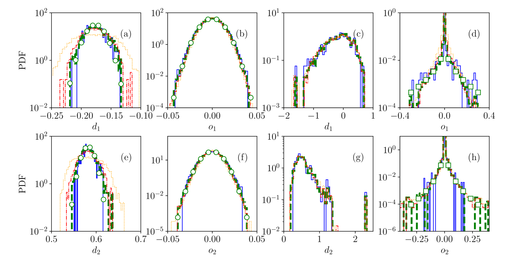
Figure 2: Histograms of the matrix elements in the diagonal blocks $\tilde{O}^{(0,0)}(\beta=0)$ for $\hat{O}_{1}$ (upper row) and $\tilde{O}^{(0,0)}(\beta=0.2)$ for $\hat{O}_{2}$ (lower row). (a), (b), (e), and (f) are for the nonintegrable case with $\lambda=1$, and the others for the integrable case with $\lambda=0$. The energy shell widths are $\Delta_{E}=0.1$ (blue solid), $0.3$ (green dashed), $0.5$ (red dashed-dotted), and $1.0$ (orange dotted). Diagonal and off-diagonal matrix elements of $\hat{O}_{i}$ are denoted as $d_{i}$ and $o_{i}$, respectively. The numerical histograms are compared with the Gaussian distribution functions (circular symbols) and the stretched exponential functions (square symbols).

III.1 Diagonal blocks

We focus on a diagonal block $\tilde{O}^{(0,0)}(\beta)$ which is characterized with $E_{\gamma\alpha}\simeq\bar{E}(\beta)$ and $\omega_{\gamma\alpha}\simeq 0$. A diagonal block includes both diagonal and off-diagonal matrix elements. Thus, one can compare the distributions of both quantities. Figure 2 presents the histograms obtained at $\beta=0.0$ for $\hat{O}_{1}$ and $0.2$ for $\hat{O_{2}}$.

Before proceeding, we remark on the effect of the energy shell size $\Delta_{E}$ (see also discussions in Ref. [27]). In Fig. 2, we compare the histograms obtained with $\Delta_{E}=0.1,~{}0.3,~{}0.5$, and $1.0$. There is a tradeoff between small and large $\Delta_{E}$. For small $\Delta_{E}$, one can study the intrinsic statistical property at a given energy scale. However, statistics becomes worse because an energy shell includes fewer eigenstates. As $\Delta_{E}$ increases, statistics becomes better but a systematic correction arises. For instance, in Fig. 2 (a) and (e), the histogram broadens as $\Delta_{E}$ increases. A diagonal element $O_{\alpha\alpha}$ is an energy eigenstate expectation value. With finite $\Delta_{E}$, the histogram is given by the superposition of the intrinsic distribution functions at different energy values. The extrinsic fluctuation due to the energy dispersion results in the broadening. In order to suppress the extrinsic fluctuation, $\Delta_{E}$ should be smaller than the energy dispersion $\delta E=O(L^{d/2})$ with dimensionality $d$ of the thermal equilibrium state. In this paper, we will use the intermediate value of $\Delta_{E}=0.3$ unless stated otherwise. The block submatrix $\tilde{O}^{(0,0)}(\beta)$ is of size $\mathcal{N}\times\mathcal{N}$ where $\mathcal{N}=1278~{}(1062)$ for $\beta=0.0~{}(0.2)$ when $\lambda=1$ and $\mathcal{N}=916~{}(741)$ for $\beta=0.0~{}(0.2)$ when $\lambda=0$.

The diagonal and off-diagonal elements of both observables follow the Gaussian distribution in the nonintegrable case. In Figs. 2(b) and (f), we compare the numerical histogram of the off-diagonal elements with the symmetric Gaussian function, represented with circular symbols, of the same variance. They are in perfect agreement. The ETH predicts that the variance of the diagonal elements is twice that of the off-diagonal elements [20, 23]. In Figs. 2(a) and (e), we compare the numerical histogram of the diagonal elements with the Gaussian function whose variance is set to a double of the variance of the off-diagonal elements. The center of the Gaussian is shifted to the mean value of the diagonal elements. The perfect agreement confirms the ETH ansatz in Eq. (1) for $\omega_{\gamma\alpha}\simeq 0$.

In the integrable case, the numerical data are not compatible with the ETH ansatz. The histograms of diagonal elements, shown in Figs. 2(c) and (g), and of off-diagonal elements, shown in Figs. 2(d) and (h), do not have the Gaussian shape. The histogram of the off-diagonal elements is fitted well with a stretched exponential function $f_{s}(x)=pe^{-q|x|^{\theta}}$, which is plotted with square symbols in Fig. 2(d) and (h). The exponent takes a value $\theta\simeq 0.47$ in Fig. 2(d) and $\theta\simeq 0.34$ in Fig. 2(h). Our numerical results suggest that the exponent may vary with $\beta$. Statistics of the off-diagonal elements of $\hat{O}_{1}$ is also investigated in Ref. [25] at different values of $\Delta$. It is reported that they may follow a log-normal distribution. A theoretical study is necessary in order to understand the nature of the offdiagonal elements in the integrable systems, which is beyond the scope of the current work.

The variance of off-diagonal elements, denoted by $\sigma^{2}_{o}[\hat{O}]$ with subscript $o$ standing for off-diagonal elements, depends on the system size $L$. We investigate the size dependence at $\beta=0.0,~{}0.1,~{}0.2$, and $0.3$. The ETH predicts that

$$\sigma^{2}_{o}[\hat{O}]=e^{-S(\bar{E})}|f_{O}(\bar{E},\omega=0)|^{2}.$$ (8)

The system size dependence comes into play through the entropy function $S(\bar{E}(\beta))$. It can be estimated as $S(\bar{E})=\ln\mathcal{D}(\bar{E})$ where $\mathcal{D}(\bar{E})=\mathcal{N}_{0}/\Delta_{E}$ is the density of the states.

The variance multiplied by $\mathcal{D}$ is plotted in Fig. 3 as a function of $\beta$. In the nonintegrable case, the curves from different system sizes $L=20,22$, and $24$ tend to align along a single curve, which corresponds to the function $|f_{O}(\bar{E}(\beta),\omega=0)|^{2}$ for the observable $\hat{O_{1}}$ or $\hat{O_{2}}$ appearing in Eq. (8). This behavior is fully consistent with the prediction of the ETH. Most of previous works investigated the scaling of the off-diagonal elements corresponding to the infinite temperature state ($\beta=0$) where $\mathcal{D}$ is proportional to the dimensionality of the total Hilbert space [20, 25, 23]. Our work confirms the scaling form of Eq. (8) at finite temperature states.

In the integrable system, the scaled variances obtained at different system sizes are rather scattered. Nevertheless, from the plots in Fig. 3(b) for $L=22$ and $24$, we expect that the off-diagonal elements of $\hat{O}_{1}$ follow the same scaling form of Eq. (8) for large enough system sizes. The data for $\hat{O}_{2}$ are more scattered. However, further analysis in the following subsection supports that the scaling form $\sigma_{o}^{2}\propto 1/\mathcal{D}$ is also valid for $\hat{O}_{2}$. Such a scaling has been also reported in the integrable XXZ model with other parameter values [25].

We remark that the scaling $\sigma^{2}_{o}\propto 1/\mathcal{D}$ should not be regarded as the evidence for the ETH. We have already shown that the off-diagonal elements in the integrable system do not follow the Gaussian distribution. What is shown in Fig. 3 is that the fluctuation amplitude of the off-diagonal elements scales as $1/\mathcal{D}$ in both integrable and nonintegrable systems.

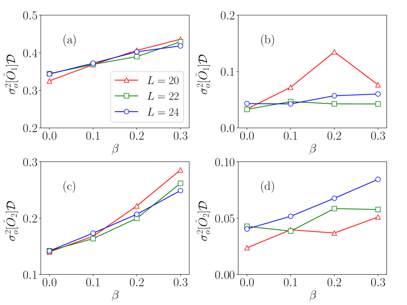
Figure 3: Scaled variance of off-diagonal elements within a diagonal block $\tilde{O}^{(0,0)}(\beta)$. The variance is multiplied by the density of states $\mathcal{D}(\bar{E}(\beta))$. (a) and (c) correspond to the nonintegrable case ($\lambda=1$), while the others corresponds to the integrable case ($\lambda=0$). The system sizes are $L=20$, $22$, and $24$.

III.2 Off-diagonal blocks

We investigate matrix elements of off-diagonal blocks $\tilde{O}^{(b,a)}(\beta)$ with $b\neq a$. As explained in Sec. II, a block submatrix $\tilde{O}^{(b,a)}(\beta)$ consists of matrix elements $\{O_{\gamma\alpha}\}$ with $E_{\alpha}\simeq\bar{E}(\beta)+a\Delta_{E}$ and $E_{\gamma}\simeq\bar{E}(\beta)+b\Delta_{E}$. Off-diagonal blocks with $b\neq a$ include only off-diagonal elements. Specifically, we will consider the block submatrices with $b=-a~{}(=1,2,\cdots)$ in which $E_{\gamma\alpha}\simeq\bar{E}(\beta)$ and $\omega_{\gamma\alpha}\simeq\omega=2b\Delta_{E}$. They are represented by the shaded squares in Fig. 1. We have measured the probability distribution and the variance at each off-diagonal block. The numerical results at $\beta=0$ and $0.2$ are presented in Fig. 4 for the nonintegrable case and Fig. 5 for the integrable case.

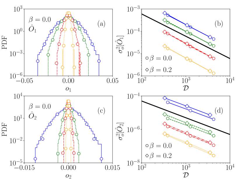
Figure 4: Numerical data for the off-diagonal blocks $\tilde{O}^{(b,-b)}(\beta)$ with $\omega=2b\Delta_{E}$ with $2b=4$ (blue solid), $8$ (green dashed), $12$ (red dashed dotted), and $16$ (orange dotted) in the nonintegrable case. (a) and (c) show the histograms for $\hat{O}_{1}$ and $\hat{O}_{2}$, respectively, at $L=24$ and $\beta=0$. Each numerical histogram is compared with the Gaussian function, marked with circular symbols, of the same variance. The variance is plotted against the density of states $\mathcal{D}(\bar{E}(\beta))$ in (b) for $\hat{O}_{1}$ and (d) for $\hat{O}_{2}$ at $\beta=0.0~{}(\circ)$ and $0.2~{}(\diamond)$. The thick straight line of slope $-1$ is a guide to the eye. The sizes of the block submatrices with $2b=4$ are $(1269\times 1226)$ at $\beta=0.0$ and $(1182\times 912)$ at $\beta=0.2$ when $L=24$. The other block submatrices are of similar size.

Non-integrable case.— At all values of $\bar{E}(\beta)$ and $\omega$ considered, off-diagonal matrix elements follow the symmetric Gaussian distribution. In Fig. 4(a) and (c), we compare the numerical histogram obtained at $L=24$ with the symmetric Gaussian function of the same variance. The agreement is almost perfect, which indicates the validity of the ETH.

The variance of the elements within $\tilde{O}^{(b,-b)}(\beta)$ at different system sizes $L=20$, $22$, and $24$ is plotted as a function of the density of states $\mathcal{D}(\bar{E}(\beta))$ in Figs. 4(b) and (d). For both observables $\hat{O}_{1}$ and $\hat{O}_{2}$, the variance is inversely proportional to the density of states at all values of $\beta$ and $\omega$. Their slopes correspond to the functions $|f_{O}(\bar{E},\omega)|^{2}$. These numerical results, together with those in the preceding subsections, strongly support the ETH ansatz in Eq. (1) at all energy scales.

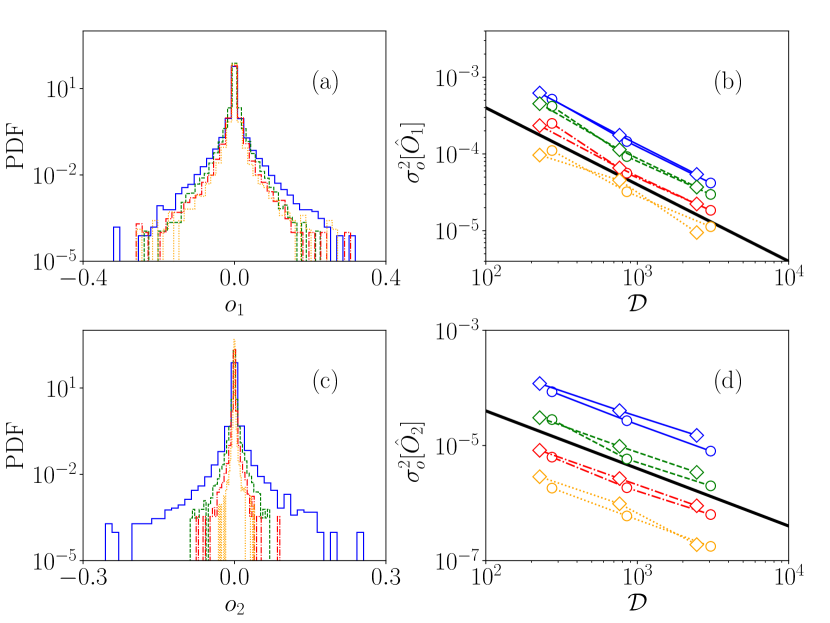
Figure 5: The same plots as in Fig. 4 for the integrable case. The sizes of the block submatrices with $2b=4$ are $(886\times 895)$ at $\beta=0.0$ and $(808\times 678)$ at $\beta=0.2$ when $L=24$.

Integrable case.– We have performed the same analysis in the integrable system. The histograms for $\hat{O}_{1}$ and $\hat{O}_{2}$ are presented in Fig. 5(a) and (c), respectively. As in the case with $\omega=0$ [Figs. 2(d) and (h)], the distribution functions are non-Gaussian. They decay more slowly than an exponential function in the tail.

We also investigate the finite-size scaling behavior of the variance. We have measured the variance of the matrix elements in each off-diagonal block $\tilde{O}^{(b,-b)}(\beta)$ at different system sizes $L=20$, $22$, and $24$. They are plotted against the density of states $\mathcal{D}(\bar{E}(\beta))$ in Figs. 5(b) and (d). The overall behavior is consistent with the scaling $\sigma^{2}_{o}(\hat{O})\propto 1/\mathcal{D}$ for both observables at all parameter values. Such a scaling was also reported for the integrable systems at the center of the energy spectrum [17, 25]. In comparison to the data shown in Fig. 4, the data suffer from stronger fluctuations. These behaviors were also observed in the diagonal blocks [see Figs. 3(b) and (d)].

In this subsection, we have investigated the statistical property of off-diagonal matrix elements $\{O_{\gamma\alpha}\}$ within each block characterized with $E_{\gamma\alpha}\simeq\bar{E}(\beta)$ and $\omega_{\gamma\alpha}\simeq\omega\neq 0$. We have confirmed that the nonintegrable system follows the prediction of the ETH in Eq. (3) with Gaussian random variables $R_{\gamma\alpha}$. In the integrable systems, off-diagonal matrix elements do not follow the Gaussian distribution. However, the variance is still inversely proportional to the density of states.

IV Eigenstate-to-eigenstate fluctuations

The ETH ansatz in Eq. (1) is a strong requirement that all matrix elements involving nearby energy eigenstates should be statistically equivalent. The equivalence for the diagonal elements has been tested by performing the finite size scaling analysis of $\delta O_{\alpha}=|O_{(\alpha+1)(\alpha+1)}-O_{\alpha\alpha}|$ [16, 19, 23] and of the deviation of eigenstate expectation values from the microcanonical ensemble average [21]. However, off-diagonal elements have been studied only at the coarse-grained level. The eigenstate-to-eigenstate fluctuations for off-diagonal elements have not been studied both for the nonintegrable and the integrable systems, which will be addressed in this section.

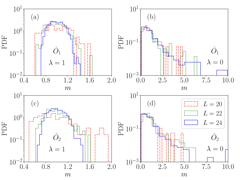
Figure 6: Histogram of the normalized columnar second moments, $m=M_{2}/\langle M_{2}\rangle$, of off-diagonal elements within a block submatrix $\tilde{O}^{(b,-b)}(\beta)$ with $\beta=0.0$ and $b=8$. When $L=24$, the sizes of the block submatrices are $(921\times 829)$ in the nonintegrable case and $(712\times 776)$ in the integrable case.

We consider a block submatrix $\tilde{O}^{(b,-b)}(\beta)$ characterized with $E_{\gamma\alpha}\simeq\bar{E}(\beta)$ and $\omega_{\gamma\alpha}\simeq\omega=2b\Delta_{E}$. A column corresponding to an energy eigenstate $|\alpha\rangle\in\mathcal{S}_{-b}$ is a set of $O_{\gamma\alpha}$’s where $|\gamma\rangle\in\mathcal{S}_{b}$ (see Fig. 1). Instead of measuring the moment of all elements in a block, we measure the second moment $M_{2}$ of the elements in a column separately. Then, we can quantify the eigenstate-to-eigenstate fluctuations from the distribution of the columnar second moments.

In Fig. 6, we present the histogram of the normalized columnar second moments $m\equiv M_{2}/\langle M_{2}\rangle$ where $\langle M_{2}\rangle$ is the mean value of the second moments of all columns within a block submatrix. In the nonintegrable case with $\lambda=1$, shown in Figs. 6(a) and (c), the distribution functions are peaked around $m\simeq 1.0$. Furthermore, the peak becomes narrower as the system size $L$ increases.

The integrable system ($\lambda=0$) exhibits distinct behaviors. The distribution functions shown in Figs. 6(b) and (d) have a long tail. Furthermore, we cannot find any signature suggesting that the width of the distribution may decrease with the system size.

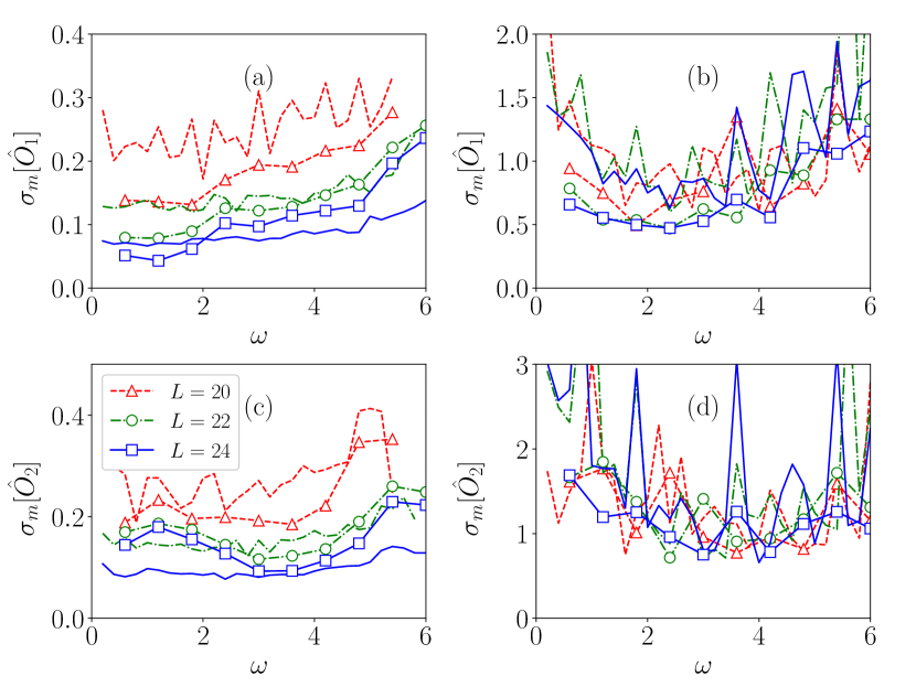
Figure 7: Standard deviation $\sigma_{m}[\hat{O}_{i}]$ of the normalized columnar second moments of off-diagonal elements in $\tilde{O}_{b,-b}(\beta=0)$. The data are plotted as a function of $\omega=2b\Delta_{E}$. Lines with symbols represent the data with $\Delta_{E}=0.3$, while lines without symbols represent the data with $\Delta_{E}=0.1$. The panels (a) and (c) are for the nonintegrable system, and (b) and (d) are for the integrable system.

We quantify the eigenstate-to-eigenstate fluctuation with the standard deviation of $m$. The numerical data are plotted in Fig. 7. In the nonintegrable case ($\lambda=1$), the standard deviation decreases as the system size increases at all values of $\omega=2b\Delta_{E}$. On the other hand, in the integrable case ($\lambda=1$), the standard deviation tends to converge to nonzero values.

We remark that there are two sources of the fluctuations leading to nonzero values of $\sigma_{m}$. First of all, any intrinsic eigenstate-to-eigenstate fluctuations, which we are interested in, are responsible for the variation of $m$. In addition, extrinsic fluctuations due to the energy dispersion of the order of $\Delta_{E}$ among eigenstates also contribute to the fluctuations. In order to reduce the effect of the extrinsic fluctuations, we have also measured the standard deviation of $m$ using the smaller values of the energy shell width $\Delta_{E}=0.1$. The two data sets from $\Delta_{E}=0.1$ and $0.3$ are compared in Fig. 7, which gives a hint on the nature of the intrinsic fluctuations. In the nonintegrable case, the relative standard deviation decays more rapidly with the system size at $\Delta_{E}=0.1$. In the integrable case, the relative fluctuation becomes even stronger at $\Delta_{E}=0.1$.

Based on the numerical results, we conclude that the intrinsic eigenstate-to-eigenstate fluctuations vanish in the nonintegrable system while they remain finite in the integrable system in the infinite size limit. Our result provides a strong support for the ETH ansatz for off-diagonal elements in the nonintegrable systems. It also reveals that the eigenstate-to-eigenstate fluctuations as well as the non-Gaussian distribution functions invalidate the ETH for off-diagonal elements in the integrable systems.

V Summary and Discussions

In summary, we have performed a thorough numerical analysis on the statistical property of matrix elements $\{O_{\gamma\alpha}\}$ of observables in the energy eigenstate basis of the integrable and the nonintegrable spin-$1/2$ XXZ chains. Using the block submatrix, we have investigated the statistical property in the energy-resolved way. Our study confirms that the ETH ansatz characterizes statistics of matrix elements in the nonintegrable model at all energy scales. In various regions with different values of $E_{\gamma\alpha}\simeq\bar{E}$ and $\omega_{\gamma\alpha}\simeq\omega$, the distribution functions are shown to follow the prediction of the ETH.

Statistics in the integrable system is subtle. Both the diagonal and off-diagonal elements do not follow the Gaussian distribution of the ETH. On the other hand, the variance of off-diagonal elements within blocks seems to be well-defined and inversely proportional to the density of states. However, we discover that the eigenstate-to-eigenstate fluctuations are relevant in the integrable system. Figures 6 and 7 show that the eigenstate-to-eigenstate fluctuations are of the same order of magnitude as the overall fluctuations, which disproves a scaling form such as in Eq. (8).

In the nonintegrable system, the eigenstate-to-eigenstate fluctuation vanishes in the large system size limit. It implies that the nonintegrable system has the self-averaging property that nearby energy eigenstates are statistically equivalent to each others. It provides a strong justification of the ETH.

The eigenstate-to-eigenstate fluctuation is important to understand the origin for the breakdown of the FDT in the integrable system. When a system is prepared initially at an energy eigenstate $\ket{\alpha}$, a dynamic correlation function $\bar{S}(\omega)=\int_{-\infty}^{\infty}dt\langle\hat{O}(t)\hat{O}(0)\rangle e^{i\omega t}$ of an observable $\hat{O}$ in the frequency domain is given by 

$$\bar{S}(\omega)=2\pi\sum_{\gamma\neq\alpha}O_{\alpha\gamma}O_{\gamma\alpha}\delta(\omega-\omega_{\gamma\alpha}).$$ (9)

In the Gibbs state, the correlation function and the response function are related through the FDT [36]. Recently, it is shown that the FDT is also valid in an energy eigenstate for the isolated quantum systems obeying the ETH [5, 9, 10]. The derivation relies on the properties that the second moment of $O_{\gamma\alpha}$’s is a smooth function of $E_{\gamma\alpha}$ and $\omega_{\gamma\alpha}$ and is inversely proportional to the density of states $\mathcal{D}(E_{\gamma\alpha})$. Interestingly, the numerical results of Sec. III.2 and the literatures, e.g., Ref. [25], show that the integrable systems have the same properties at the coarse-grained level. It is puzzling because the FDT is violated in the integrable systems [30, 31]. This puzzle is resolved by the eigenstate-to-eigenstate fluctuations.

The FDT can be casted in the form of the Kubo-Martin-Schwinger (KMS) relation [36, 37]

$$\bar{S}(\omega)=e^{\beta\omega}\bar{S}(-\omega).$$ (10)

It constrains that $\frac{1}{\omega}\ln[\bar{S}(\omega)/\bar{S}(-\omega)]$ should depend only on the inverse temperature $\beta$. It should be independent of $\omega$ and the eigenstate quantum number $\alpha$. The correlation function $\bar{S}(\omega)$ in Eq. (9) involves a columnar second moment. In the presence of the eigenstate-to-eigenstate fluctuations, the columnar second moment has an explicit eigenstate dependence, which results in $\omega$ and $\alpha$ dependence of $\frac{1}{\omega}\ln[\bar{S}(\omega)/\bar{S}(-\omega)]$ in general. It explains the reason why the FDT is violated in the integrable systems.

The eigenstate-to-eigenstate fluctuations presented in Fig. 7 depend on the choice of $\Delta_{E}$. In order to reduce the effect of the extrinsic fluctuations and achieve a good statistics, one need to choose a smaller value of $\Delta_{E}$ at larger system sizes. We leave a more quantitative study on the finite size scaling property at larger systems as a future work.