Planckian relaxation delusion in metals

Abstract

We present a critical review of recent attempts to introduce the new quantum (“Planckian”) limit for the temperature dependence of inelastic scattering rate of electrons in metals. We briefly discuss the main experimental facts and some simple theoretical models explaining the linear in temperature growth of resistivity (starting from very low temperatures) in superconducting cuprates and some similar systems. There is no commonly accepted theoretical explanation of such behavior up to now. We also discuss the known quantum limits for electrical conductivity (resistance). It is shown that the universal Planckian limit for the inelastic relaxation rate proposed in some papers is a kind of delusion related to a certain procedure to represent the experimental data.

I Introduction

Linear in temperature ($T$ – linear) growth of electrical resistivity of cuprates and some other correlated systems in the wide temperature region from pretty low to rather high temperatures remains among the most challenging problems of the physics of high – temperature superconductors for many years. Observed in cuprates since the early experiments Batl ; Iye it became one of the marked properties of these compounds in normal phase, starting in optimally doped systems from the temperature of superconducting transition $T_{c}$ and continuing up to highest temperatures achievable before destruction the samples. Later the similar behavior of resistivity was observed in some other similar systems. By itself, the $T$ – linear growth of resistivity in metals is not at all surprising, it is observed practically always, though at high enough temperatures $T>\Theta_{D}/5$, where $\Theta_{D}$ – is Debye temperature, which is usually some hundreds of degrees. What is surprising is the fact, that the $T$ – linear growth in cuprates takes place, starting from significantly lower temperatures. The commonly accepted explanation of such behavior is still lacking, though during these years a number of theoretical models were proposed, claiming such explanation. But this is not the aim of the current work.

The thing is that recently a number of interesting papers appeared Bruin ; Legros , where after rather detailed analysis of a wide experimental material on many compounds, it was shown that in the $T$ – linear region of resistivity, the scattering rate of electrons (inverse relaxation time) is pretty accurately described by the dependence $\Gamma(T)=1/\tau=\alpha k_{B}T/\hbar$, where $\alpha\sim 1$ and is weakly varying from one material to another. In particular, for systems in the vicinity of quantum critical points (on the phase diagram of cuprates and some similar systems) the value of $\alpha$ is in the interval of 0.7 – 1.1, and is seemingly universal and independent of the strength of interaction, leading to relaxation of electronic current. More so, it was discovered that the similar dependence gives rather good description of the data for a number of usual metals (like Cu, Au, Al, Ag, Pb, Nb etc.) in the $T$ – linear region of their resistivity. In this case the values of $\alpha$ belong to noticeably wider interval from 0.7 to 2.7 Bruin ; Legros . In connection with these (and similar) results the concept of the universal (independent of interaction strength) “Planckian” upper limit of scattering rate $\frac{1}{\tau_{P}}=\Gamma_{P}\sim\frac{k_{B}T}{\hbar}$ was introduced in Ref. Zaanen .

Below we shall present a short review of the relevant experimental data and discuss some theoretical models, imposing quantum limitations on resistivity of metals, with the aim to understand the degree of validity of the concept of “Planckian” relaxation in metals.

II Experiments

Temperature dependence of resistivity at low enough temperatures ($T<0.2\Theta_{D}\ll E_{F}$, $\Theta_{D}$ – Debye temperature, $E_{F}$ – Fermi energy) is described by the following expression:

$$\rho(T)=\rho_{0}+\rho_{T}(T)=\rho_{0}+a_{ee}\left(\frac{k_{B}T}{E_{F}}\right)^{2}+a_{ep}\left(\frac{T}{\Theta_{D}}\right)^{5}$$ (1)

where $\rho_{0}$ – is residual resistivity at zero temperature due to impurity scattering, the second term is the contribution electron – electron scattering, while the third one is the low temperature contribution from electron – phonon scattering, described by Bloch – Grüneisen theory Zim . For high enough temperatures $T>0.2\Theta_{D}$ this theory gives:

$$\rho(T)-\rho_{0}=AT$$ (2)

This behavior of resistivity is clearly seen in the experiments, as shown in Fig. 1, where we show the data for a number of simple metals Meiss . These results show that the temperature dependence of resistivity (conductivity) is almost totally related to the processes of inelastic scattering by phonons. In case of significant contribution of scattering by other collective excitations, e.g. spin fluctuations, we can write down in fact very similar expressions.

From these data it is seen, that for temperatures $T>\Theta_{D}/5$ resistivity of a metal grows linearly with temperature. In most metals $\Theta_{D}\sim$ 200–600K.

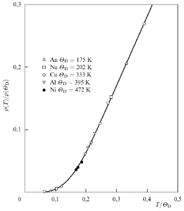
Figure 1: Temperature dependence of resistivity for typical metals. Meiss

At the same time, the critical temperature of superconducting transition in cuprates is commonly some dozens of degrees, so that $T_{c}\sim\Theta_{D}/5$. Thus, for rather long time there was a hope Maks that $T$ – linear growth of resistivity in cuprates can be explained by the usual electron – phonon scattering, taking into account that it takes place outside the region of low temperature power – like growth, which is masked by superconducting transition. There were some cases of few exceptional samples with low values of $T_{c}$, where $T$ – linear growth of resistivity was observed starting from anomalously low temperatures $T<10$K Fior , but these were rather seldom. There were no experiments in the normal phase at low enough temperatures simply because the destruction of superconducting state in typical cuprates required extremely high magnetic fields.

This situation changed in recent years after such experiments were successfully performed Bruin ; Legros . These works presented the data on resistivity in a number of high – temperature cuprate superconductors as well as on some analogous systems in very high magnetic fields, suppressing superconductivity. The detailed analysis of these experiments and data obtained by other authors has shown that $T$ – linear behavior of resistivity is conserved in normal phase, in many cases, up to the lowest temperatures.

Typical examples of experimental data from Refs. Bruin ; Legros are shown in Fig. 2, 3, 4. In these works, characterized by the very detailed analysis of experimental situation, many additional data can be found. These results aggravated further the question of the nature of $T$ – linear resistivity in systems under consideration. It should be stressed from the very beginning, that this problems remains unsolved up to now and this is not the aim of the present work.

For us the main interest now is the analysis of experimental data presented in Refs. Bruin ; Legros , which allowed the authors to determine the temperature dependence of relaxation time $\tau$, from the values of resistivity and to come to rather unexpected results and conclusions.

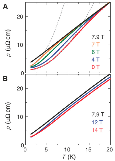
Figure 2: (A) Resistivity $\rho$ as function of temperature $T$ of very pure single crystal of Sr₃Ru₂O₇ in magnetic fields 0T (red line), 4T (blue), 6T (green), 7T (orange) and in critical field $H_{c}$=7.9T (black), corresponding to quantum critical point ($H_{c}$,$T=0$). Dashed lines – a fit to $\rho_{0}+AT^{2}$ dependence at low temperatures, which demonstrates the narrowing of the region of quadratic dependence on temperature and crossover to linear dependence. Bruin (B) Temperature dependence of resistivity $\rho$ in fields $H_{c}$ (black), 12T (blue) and 14T (red). Bruin

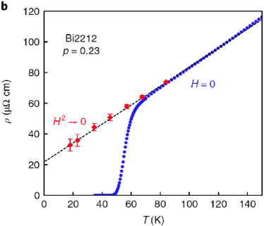
Figure 3: Resistivity of Bi2212 thin film as function of temperature for $H=$0 (blue curve). Red dots (and dashed line) show resistivity in normal phase for $T<T_{c}$, obtained by suppressing superconductivity by external magnetic field and extrapolation from $\rho=a+bH^{2}$ dependence. Legros

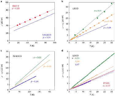
Figure 4: Linear in temperature dependence of resistivity in overdoped cuprates, showing the behavior of $\rho$ in highly – conducting plane (i.e. $\rho_{ab}$) in (a) Nd-LSCO for $p=0.24$ (blue line, $H=$16T) and Bi2212 for $p=$0.23 (red symbols), $H=$55T); (b) $\rho(T)-\rho_{0}$ in LSCO for $p=$0.21 (green symbols, $H=$48T) and $p=$0.23 (orange, $H=$48T), $p=$0.26 (blue, $H=$18T); (c) $\rho(T)-\rho_{0}$ in Nd-LSCO at $H=$33T for $p=$0.22 (green), $p=$0.23 (orange) and $p=$0.24 (blue); (d) $\rho(T)-\rho_{0}$ in LCCO for $x=$0.16 (orange, $H=$6.5T) and $x=$0.17 (blue, $H=$4T) and PCCO for $x=$0.17 (red, $H=$16T). Legros

The main idea of the analysis performed in Refs. Bruin ; Legros was as follows. Let us write down the Drude expression for conductivity as:

$$\sigma=\frac{ne^{2}\tau}{m^{\star}}=\frac{ne^{2}v_{F}\tau}{\hbar k_{F}}$$ (3)

where $v_{F}$ is electron velocity at Fermi surface, $m^{\star}$ is an effective mass, $p_{F}=m^{\star}v_{F}=\hbar k_{F}$ is Fermi momentum. Correspondingly for resistivity we have:

$$\rho=\frac{m^{\star}}{ne^{2}\tau}=\frac{\hbar k_{F}}{ne^{2}v_{F}\tau}$$ (4)

The effective mass $m^{\star}$ or the value of $\hbar k_{F}/v_{F}$ in Refs. Bruin ; Legros were determined from electronic contribution to specific heat, which can be measured at low temperatures, or from the measurements of de Haas – van Alfen effect, which are also made at low enough temperatures. These measurements in fact determine the value of the effective mass $m^{\star}$ and Fermi wave – vector $k_{F}$ as some average values for each of the pockets of the Fermi surface.

Electron density $n$, entering these expressions can be calculated (for systems of different dimensionality) as:

$$n=\frac{2k_{F}}{\pi d_{b}d_{c}}\qquad\mbox{(quasi-one-dimensional case)}$$ (5)

$$n=\frac{k_{F}^{2}}{2\pi d}\qquad\mbox{(quasi-two-dimensional case)}$$ (6)

$$n=\frac{k_{F}^{3}}{3\pi^{2}}\qquad\mbox{(three-dimensional case)}$$ (7)

where $d_{b}$ and $d_{c}$ are the distances between adjacent conducting chains (oriented along $a$-axis) in the directions of $b$ and $c$-axis in quasi – one – dimensional system, while $d$ is the distance between adjacent conducting planes in quasi – two – dimensional case.

If we express the temperature – dependent part of resistivity as in (2) and introduce the $T$ – linear (Planckian) relaxation rate as:

$$\Gamma=\frac{1}{\tau}=\alpha\frac{k_{B}T}{\hbar};\quad\alpha\sim const$$ (8)

we immediately obtain:

$$A=\frac{d\rho}{dT}=\alpha\frac{k_{B}}{\hbar}\frac{m^{\star}}{ne^{2}}\quad\mbox{or}$$ (9)

$$\frac{ne^{2}}{k_{B}k_{F}}\frac{d\rho}{dT}=\alpha\frac{m^{\star}}{\hbar k_{F}}=\frac{\alpha}{v_{F}}$$ (10)

which gives working formulae to represent experimental data in $T$ – linear region of resistivity Bruin ; Legros .

In Refs. Bruin ; Legros the very detailed analysis of experimental data was performed for rather wide set of systems (compounds) with very different electronic structures, from high – temperature superconducting copper oxides and iron based superconductors to organic metals like (TMTSF)₂PF₆, through to compounds like Sr₃Ru₂O₇, CeCoIn₅, UPt₃, CeRu₂Si₂, where the $T$ – linear growth of resistivity is observed.

It was discovered, that for all these quite different systems, the experimental data for thus defined relaxation rate are well described by dependence like (8) and the value of $\alpha$ for majority of these systems belong to the interval 0.7 – 1.1, and seems to be universal (independent of peculiarities of electronic spectrum or the strength of interaction, leading to scattering of electrons). More so, it was also shown, that the similar dependence is appropriately describing also the data for a number of usual metals (Cu, Au, Al, Ag, Pb, Nb), though the values of $\alpha$ for them belong to a wider interval from 0.7 to 2.8 Bruin ; Legros .

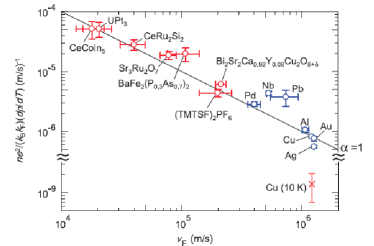
Figure 5: The general picture for different metals (different Fermi velocities $v_{F}$), demonstrating the the $T$ – linear growth of resistivity. These metals include heavy – fermion systems, oxides, pnictides and organic metals, where the $T$ – linear growth of resistivity at low temperatures appears after the application of magnetic field, change of the chemical composition or external hydrostatic pressure. Analogous data represent the situation in common metals with $T$ – linear behavior of resistivity at high enough temperatures (blue symbols), while for lower temperatures their resistivity is orders of magnitude smaller (appropriate value for Cu at $T=$10K is shown in right lower corner). Straight line, denoted by $\alpha=1$, corresponds to $(\tau T)^{-1}=k_{B}/\hbar$. Legros

In the Table given below we show, as an example, the experimental values of some parameters under discussion, determined in Ref. Legros , for a number of quasi – two – dimensional systems (hole doped and electron doped cuprates, organics).

Compound	Doping	$n$(1027m-3)	$m^{\star}/m_{0}$	$A/d$($\Omega$ K-1)	$\alpha$
Bi2Sr2CaCu2O8-δ (Bi2212)	$p=$0.23	6.8	8.4$\pm$1.6	8.0$\pm$0.9	1.1$\pm$0.3
Bi2Sr2CuO6+δ (Bi2201)	$p=$0.4	3.5	7$\pm$1.5	8$\pm$2	1.0$\pm$0.4
La2-xSrxCuO4 (LSCO)	$p=$0.26	7.8	9.8$\pm$1.7	8.2$\pm$1.0	0.9$\pm$0.3
La1.6-xNd0.4SrxCuO4 (Nd-LSCO)	$p=$0.24	7.9	12$\pm$4	7.4$\pm$0.8	0.7$\pm$0.4
Pr2-xCexCuO4±δ (PCCO)	$x=$0.17	8.8	2.4$\pm$0.1	1.7$\pm$0.3	0.8$\pm$0.2
La${}_{2-x}Ce$xCu)4 (LCCO)	$x=0.15$	9.0	3.0$\pm$0.3	3.0$\pm$0.45	1.2$\pm$0.3
(TMTSF)2PF6 (TMTSF)	$P=$11kbar	1.4	1.15$\pm$0.2	2.8$\pm$0.45	1.0$\pm$0.3

In Refs. Bruin ; Legros further details can be found on similar data for all systems mentioned above.

All this is nicely illustrated by consolidated graph shown in Fig. 5, where data are shown in logarithmic scale representing Eq. (10). These results seem to be quite nontrivial and apparently confirm the concept of universal “Planckian” mechanism of electronic relaxation in metals, which was introduced earlier Zaanen and applied to cuprates physics. More so, the value of $\alpha\sim 1$, which is observed for such a wide set of materials with very different electronic spectra and quite different Fermi surfaces, suggests the idea that (8) is actually the universal quantum upper limit for inelastic (temperature – dependent) relaxation rate for electrons in metals.

To explain such temperature behavior of resistivity for so different systems, from the lowest temperatures, a number of complicated theoretical models was proposed recently Khod ; Khodel ; Sachdev ; Vol , including some very exotic, taken from the physics of black holes, cosmology and superstring theory (cf. Zan ; Hart ; Herz ; Hartn ). Below we shall limit ourselves to a simple analysis based on the traditional approaches of quantum theory of solids.

III Quantum estimates for resistivity of metals.

Let us remind some elementary theoretical estimates with respect to conductivity (resistivity) of metals. Drude expressions for elastic and inelastic scattering are written as:

$$\sigma_{0}=\frac{ne^{2}}{m}\tau_{0};\qquad\rho_{0}=\frac{m}{ne^{2}}\frac{1}{\tau_{0}}$$ (11)

$$\sigma_{i}(T)=\frac{ne^{2}}{m}\tau(T);\qquad\rho_{i}(T)=\frac{m}{ne^{2}}\frac{1}{\tau(T)}$$ (12)

where $\tau_{0}$ – is the mean free time due to elastic impurity scattering, determining the residual resistivity, and $\tau(T)$ is relaxation time due to inelastic scattering by phonons (or some other collective excitations), or due to electron – electron scatterings. Mass $m$ here is always understood as free electron mass (band structure mass in a solid!), which does not include corrections due to electron – electron or electron – phonon interactions (see more details below). Then, assuming the additive contributions of different scattering mechanisms (Matissen rule), the total resistivity is written as:

$$\rho(T)=\frac{m}{ne^{2}}\left(\frac{1}{\tau_{0}}+\frac{1}{\tau(T)}\right)\equiv\frac{m}{ne^{2}}(\Gamma_{0}+\Gamma(T))$$ (13)

where we have introduced the appropriate scattering rates:

$$\Gamma_{0}=\frac{1}{\tau_{0}}$$ (14)

$$\Gamma(T)=\frac{1}{\tau(T)}$$ (15)

In general theory of interacting fermions (electrons) by the order of magnitude we have $\Gamma\sim Im\Sigma$, where $\Sigma$ is an electron self – energy, taking into account all the relevant interactions. Consistent approach to calculation of conductivity (resistivity) requires, of course, the treatment of a full two – particle Green’s function Diagram .

III.0.1 Ioffe – Regel limit

The most prominent quantum limitation for conductivity (resistivity) of metals is the Ioffe – Regel limit IR , which is relevant to strongly disordered systems. For $T=0$ we have:

$$\sigma_{0}=\frac{ne^{2}}{m}\tau_{0}=\frac{ne^{2}}{p_{F}}l$$ (16)

where $l=v_{F}\tau_{0}$ is the mean free path. The usual kinetic theory is valid for $p_{F}l/\hbar\gg 1$ or $E_{F}\tau_{0}/\hbar\gg 1$. Taking into account $n=\frac{p_{F}^{3}}{3\pi^{2}\hbar^{3}}$ we get the estimate for conductivity in the Ioffe – Regel limit as: $p_{F}l_{el}/\hbar\sim 1$ or $E_{F}\tau_{0}/\hbar\sim 1$:

$$\sigma_{IR}=\frac{e^{2}p_{F}}{3\pi^{2}\hbar^{2}}\sim\frac{e^{2}}{3\pi^{2}\hbar a}$$ (17)

where $a\sim n^{-3}$ is the average distance between electrons. For typical metallic densities $a$ is of order of interatomic distance (lattice constant). In this case (for $n\sim$10²³ cm^-3) corresponding resistivity $\rho_{IR}=\sigma_{IR}^{-1}\sim$150–300 $\mu\Omega$ cm. For majority of usual (“good”) metals, e.g. for Cu, $\rho(T=300$K)$\sim$ 1 $\mu\Omega$ cm, so that this limit remains unachievable even at highest temperatures, not exceeding the melting temperature. However, this is not so in strongly disordered (highly – resistive) alloys, where the resistivity can approach the Ioffe – Regel limit.

An estimate quite close to (17) was also proposed by Mott for the so called “minimal metallic conductivity” $\sigma_{c}$, at which (achieved as disorder grows e.g. mean free path being reduced) a discontinuous metal – insulator transition takes place at $T=0$ (Anderson localization) Mott . In fact, as it is shown in scaling theory of localization AALR ; Sad80 , this transition is continuous and $\sigma_{c}$ play a role of characteristic conductivity scale in the vicinity of Anderson transition ($2<d<4$ – space dimensionality):

$$\sigma\sim\sigma_{c}\left(\frac{l-l_{c}}{l_{c}}\right)^{(d-2)\nu}$$ (18)

where $\sigma_{c}\sim{e^{2}}/{\hbar a^{d-2}}$ and the critical value of the mean free path can be estimated from $p_{F}l_{c}/\hbar\sim 1$, i.e. $l_{c}\sim a$. Here we introduced the critical exponent of localization length, which in self – consistent theory of localization Diagram ; VW is given by:

$$\nu=\frac{1}{d-2}$$ (19)

so that $\nu=1$ for $d=3$. The modern numerical calculations of Anderson transition give the values of $\nu$ in the interval 1.5–1.8 Markos . For us not these details are important, but the fact of continuous nature of this transition, and nonexistense of any critical level of conductivity (resistivity).

Strictly speaking these estimates are valid only for $T=0$, when Anderson transition is a well – defined quantum phase transition in a system of noninteracting electrons. At finite temperatures and with the account of electron – electron interactions the situation is much more complicated and we shall not discuss it here.

In most cases the growth of resistivity with temperature slows down and saturates as resistivity approaches the Ioffe – Regel limit Gant . For such strongly disordered metals In such strongly disordered metals (highly – resistive alloys) an empirical Mooij rule is at work – after the achievement of resistivity level (at low temperatures) of the order of $\rho_{IR}$, the temperature dependence of resistivity becomes very weak and in a wide temperature interval from low to room temperatures and even higher it is often observed that the temperature coefficient of resistivity becomes negative Mooij ; Gant . This fact up to now does not have a commonly accepted explanation.

There is a common belief, that this is not so in “strange” metals like high – temperature superconducting copper oxides Gur ; Tak (in the region of optimal doping) and in a number of other systems Huss , there the $T$ – linear growth of resistivity continues even after overpassing the values of the order of $\rho_{IR}=\sigma_{IR}^{-1}\sim$ 100–300 $\mu\Omega$ cm, up to highest possible temperatures $T\sim$1000 K. However, here we always face the problem of the correct estimate of resistivity in Ioffe – Regel limit. From the estimates given above it becomes clear that it depends significantly on concentration of current carriers (which in cuprates is much lower, than in usual metals), so that e.g. for $n\sim$10²¹ cm${{}^{-}3}$ we obtain $\rho_{IR}\sim$1–10 m$\Omega$ cm. In recent experiments of weakly doped cuprates Greene it was clearly shown, that their resistivity saturates at $\rho_{IR}\sim$3–5 mOhm cm, in complete accordance with concentration of carriers, obtained from the measurements of Hall effect (at $T\sim$300 K). Thus it is quite possible, that in the experiments cited above on optimally doped cuprates the correct value of Ioffe – Regel limit was simply not achieved up to highest possible temperatures (before the destruction of samples).

However, our main interest in the following will be related to resistivity of “pure” enough metals in $T$ – linear region.

III.0.2 Planckian relaxation

The idea of Planckian relaxation mechanism in metal at high enough temperatures seems to be very attractive. Let us give some elementary arguments making it seemingly justified and based upon quite general quantum mechanical estimates using uncertainty principle Hart . At finite temperatures $T>0$ different processes of inelastic scattering (electron – phonons, interaction with spin – fluctuations etc.) are at work. Precisely these processes are responsible for establishing thermodynamic equilibrium in electronic system – the Fermi distribution. In a system of interacting particles at finite temperatures the particle (electron) distribution function is qualitatively of the same form Diagram . Conductivity of a metal (degenerate case) is determined by electron distribution in a layer $\sim k_{B}T$ around the Fermi level (chemical potential). Let us make an elementary estimate using time – energy uncertainty relation:

$$\Delta E\tau>\hbar$$ (20)

where $\tau$ is the life – time of a quantum state, while $\Delta E$ is the uncertainty of its energy. In our case $\tau=\tau(T)$ and it seems natural to take $\Delta E\sim k_{B}T$, so that we immediately obtain an estimate:

$$\Gamma(T)=\frac{1}{\tau(T)}<\alpha\frac{k_{B}T}{\hbar}\equiv\Gamma_{P}=\frac{1}{\tau_{P}}$$ (21)

where $\alpha\sim 1$. Now it is evident that according to this elementary estimate the Planckian relaxation defines an upper limit for resistivity due to inelastic scatterings:

$$\rho(T)-\rho_{0}=\frac{m}{ne^{2}}\Gamma(T)<\frac{m}{ne^{2}}\alpha\frac{k_{B}T}{\hbar}\equiv\rho_{P}(T)$$ (22)

Obviously, this estimate is of rather speculative nature for the system of many, in general, strongly interacting particles, but it correlates well with the results of experiments described above.

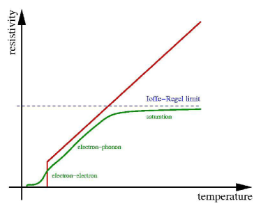
Figure 6: “Planckian” limit of electrical resistivity. Zaane Red line – the Planckian limit, green line – the usual temperature dependence of resistivity in metals.

If there exists such universal upper limit for relaxation rate, the qualitative picture of the temperature dependence of resistivity of metals can be suggested as shown in Fig. 6 Zaane . The idea here is that in “usual” metals all the temperature dependence of resistivity develops below the Ioffe – Regel limit, while the “Planckian” limit is achieved in unusual systems like HTSC – cuprates, which are near the quantum critical point and where the Ioffe – Regel limit may be surpassed with the growth of the temperature (however see Ref. Greene ).

From the estimates given above it is easy to derive the ratio of “Planckian” resistivity to that of Ioffe – Regel:Hart

$$\frac{\rho_{P}(T)}{\rho_{IR}}\sim\frac{k_{B}T}{E_{F}}$$ (23)

so that this limit may be exceeded for $k_{B}T>E_{F}$, which can be realized experimentally only in systems with low enough values of $E_{F}$ (low carrier concentration), such as copper oxides or in multiple band systems (with several pockets of the Fermi surface). In any case, according to this picture resistivity does not exceed the upper limit, determined by the “Planckian” relaxation rate, which is achieved in “strange” metals. It is quite surprising that the experimental data quoted above seem to confirm the achievement of this limit for many (!) metals, including some quite “usual”.

III.0.3 Electron – phonon interaction

Consider the most important for the theory of metals case – the electron – phonon interaction, which will be described within Eliashberg – McMillan theory, as the modern generalization of Bloch – Grüneisen theory Allen . Within this theory, the high – temperature ($T>\Theta_{D}/5$) phonon contribution to resistivity is given by Alle ; Savr :

$$\rho_{ph}(T)=\frac{4\pi mT}{ne^{2}\hbar}\int_{0}^{\infty}\frac{d\omega}{\omega}\alpha_{tr}^{2}(\omega)F(\omega)=\frac{2\pi mT}{ne^{2}\hbar}\lambda_{tr}$$ (24)

where $\alpha_{tr}^{2}(\omega)F(\omega)$ is the transport Eliashberg – McMillan function Alle ; Savr ($F(\omega)$ is the phonon density of states), determining the transport electron – phonon coupling constant as:

$$\lambda_{tr}=2\int_{0}^{\infty}\frac{d\omega}{\omega}\alpha_{tr}^{2}(\omega)F(\omega)$$ (25)

For majority of metals we have $\alpha_{tr}^{2}\approx\alpha^{2}$, where Savr

$$\lambda=2\int_{0}^{\infty}\frac{d\omega}{\omega}\alpha^{2}(\omega)F(\omega)$$ (26)

is Eliashberg – McMillan coupling constant Allen , determining the temperature of superconducting transition. Then we get a simple estimate:

$$\rho_{ph}(T)\approx\frac{2\pi mT}{ne^{2}\hbar}\lambda\equiv 2\pi\lambda\rho_{P}(T)$$ (27)

where in the last equality in the definition of $\rho_{P}(T)$ from (22) we put $\alpha=1$. In fact the values of $\lambda>1$ are not very rare in metals Allen and it becomes clear, that even the usual electron – phonon interaction can easily break the Planckian limit, so that $\rho_{ph}(T)>\rho_{P}(T)$ doses not seem exotic. This simple example immediately casts certain doubts in universality of “Planckian” relaxation, though it seems that our arguments, based on uncertainty principle, must work for any systems and interactions. However, this simple example just contradicts it.

IV Elementary model of scattering by quantum fluctuations in metals

IV.0.1 Scattering by quantum fluctuations

Here, following mainly Ref. Sad20 , we shall consider an elementary, though realistic enough, model of electron scattering by quantum fluctuations, which will allow us analyze our problem in rather general form. Consider the usual Hamiltonian of electrons in a metal interacting with some Bose – like quantum fluctuations of some arbitrary nature ($N$ is her the total number of atoms in a crystal):

$$H_{int}=\frac{1}{\sqrt{N}}\sum_{\bf pq}g_{\bf q}a^{+}_{\bf p+q}a_{\bf p}\rho_{\bf q}$$ (28)

where we have used the standard notations of creation and annihilation operators of electrons, $\rho_{\bf q}$ is an operator of quantum fluctuation of “any kind” (e.g. density of ions in a solid or collective excitations of electronic subsystem, including spin excitations, though spin indices are dropped for brevity). Let us introduce the appropriate (Matsubara time) Green’s function as Pin :

$$F({\bf q},\tau)=-<T_{\tau}\rho_{\bf q}(\tau)\rho^{+}_{\bf q}(0)>$$ (29)

Then we can write down the usual spectral representation for it as AGD :

$$F({\bf q},i\omega_{m})=\int_{-\infty}^{\infty}d\omega\frac{A({\bf q},\omega)}{i\omega_{m}-\omega}$$ (30)

where $\omega_{m}=2\pi mT$, and the spectral density is defined as:

$$A({\bf q},\omega)=Z^{-1}\sum_{mn}e^{-\frac{E_{n}}{T}}|(\rho_{\bf q})_{nm}|^{2}\left(1-e^{-\frac{\omega_{mn}}{T}}\right)\delta(\omega-\omega_{mn})$$ (31)

where $\omega_{mn}=E_{m}-E_{n}$, $(\rho_{\bf q})_{nm}=<n|\rho_{\bf q}|m>=(\rho^{+}_{\bf q})_{mn}$, and $m$, $n$ enumerate the exact many – particle states of the system.

Dynamic structure factor of fluctuations is defined as Pin ; PinNoz :

$$S({\bf q},\omega)=Z^{-1}\sum_{mn}e^{-\frac{E_{n}}{T}}|(\rho_{\bf q})_{nm}|^{2}\delta(\omega-\omega_{mn})$$ (32)

Comparing (31) and (32) we obtain:

$$A({\bf q},\omega)=S({\bf q},\omega)\left[1-e^{-\frac{\omega}{T}}\right]$$ (33)

Figure 7: Second order diagram for electron self – energy. Dashed line represents the Green’s function of a quantum fluctuation $F$, continuous line represents the electronic Green’s function $G$.

Electron Green’s function in Matsubara representation is written in a standerd form:

$$G(\varepsilon_{n},{\bf p})=\frac{1}{i\varepsilon_{n}-\xi_{\bf p}-\Sigma(\varepsilon_{n},{\bf p})}$$ (34)

where $\varepsilon_{n}=(2n+1)\pi T$, $\xi_{\bf p}$ is the free – electron spectrum counted from the Fermi level (chemical potential), and self – energy part can be taken in the simplest approximation shown by diagram in Fig. 7:

$$\Sigma(\varepsilon_{n},{\bf p})=-\frac{T}{N}\sum_{\bf q}g^{2}_{\bf q}\sum_{m}F({\bf q},i\omega_{m})G(\varepsilon_{n}+\omega_{m},{\bf p+q})$$

$$=-\frac{T}{N}\sum_{\bf q}g^{2}_{\bf q}\sum_{m}\int_{-\infty}^{\infty}d\omega\frac{S({\bf q},\omega)}{i\omega_{m}-\omega}\left(1-e^{-\frac{\omega}{T}}\right)\times$$

$$\times\frac{1}{i\varepsilon_{n}+i\omega_{m}-\xi_{\bf p+q}}$$ (35)

where $g_{\bf q}$ is the coupling constant (matrix element of interaction potential).

Consider now the case when the average frequency of fluctuation $<\Omega>$ is much lower than the temperature $T$, i.e. the classic limit for fluctuations. Then in Eq. (35) it is sufficient to take into consideration only the term with $m=0$, going actually to the picture of quasi – elastic scattering by fluctuations:

$$\Sigma(\varepsilon_{n},{\bf p})=\frac{1}{N}\sum_{\bf q}g^{2}_{\bf q}\int_{-\infty}^{\infty}d\omega\frac{S({\bf q},\omega)}{i\varepsilon_{n}-\xi_{\bf p+q}}=$$

$$=\sum_{\bf q}g^{2}_{\bf q}S({\bf q})\frac{1}{i\varepsilon_{n}-\xi_{\bf p+q}}$$ (36)

where we have introduced the structure factor of fluctuations PinNoz :

$$S({\bf q})=\frac{1}{N}\int_{-\infty}^{\infty}d\omega S({\bf q},\omega)$$ (37)

In fact, this is in a direct analogy with the well–known Ziman – Edwards approximation in the theory of liquid metals Ziman ; Edw . The case of $S({\bf q})=const$ corresponds to totally chaotic distribution of static scattering centers Diagram .

IV.0.2 Phonons

In case of scattering by phonons fluctuation operator $\rho_{\bf q}$ can be expressed via (Bose) creation and annihilation operators of phonons as PinNoz :

$$\rho_{\bf q}=\frac{1}{\sqrt{2}}\left(b^{+}_{\bf q}+b_{-\bf q}\right)$$ (38)

Then:

$$S({\bf q},\omega)=Z^{-1}\sum_{m}e^{-\frac{E_{m}}{T}}\left[<m|b_{\bf q}b^{+}_{\bf q}|m>\delta(\omega-\omega_{\bf q})+\right.$$

$$\left.+<m|b^{+}_{-\bf q}b_{-\bf q}|m>\delta(\omega+\omega_{\bf q})\right]$$

(39)

where $\omega_{\bf q}$ is phonon spectrum. Introducing the usual Bose distribution:

$$n_{\bf q}=Z^{-1}\sum_{m}e^{-\frac{E_{m}}{T}}<m|b^{+}_{\bf q}b_{\bf q}|m>=\frac{1}{e^{\frac{\omega_{\bf q}}{T}}-1}$$ (40)

we get PinNoz

$$S({\bf q},\omega)=\left[(n_{\bf q}+1)\delta(\omega-\omega_{\bf q})+n_{\bf q}\delta(\omega+\omega_{\bf q})\right]+$$

$$+\delta(\omega-\omega_{\bf q})+n_{\bf q}\left[\delta(\omega-\omega_{\bf q})+\delta(\omega+\omega_{\bf q})\right]$$ (41)

Under the conditions of $T\gg\omega_{\bf q}$, we go to the classical limit (equipartition theorem):

$$n_{\bf q}=\frac{T}{\omega_{\bf q}}$$ (42)

and accordingly

$$S({\bf q})=\frac{2T}{\omega_{\bf q}}$$ (43)

Thus we obtain the structure factor linearly growing with temperature, while its momentum dependence is determined by phonon spectrum. Then:

$$\Sigma(\varepsilon_{n},{\bf p})=T\sum_{\bf q}\frac{2g_{\bf q}^{2}}{\omega_{\bf q}}\frac{1}{i\varepsilon_{n}-\xi_{\bf p+q}}$$ (44)

To simplify the model further, let us assume the the phonon spectrum is dispersionless (Einstein phonon or optical phonon with very weak dispersion), taking $\omega_{\bf q}=\Omega_{0}$. Then performing all calculations as in the problem of an electron in a system of random impurities Diagram , we get:

$$\Sigma(\varepsilon_{n},{\bf p})=-i\pi sign\varepsilon_{n}\frac{2g_{0}^{2}}{\Omega_{0}}N(0)T$$ (45)

where $N(0)$ is the density of states on the Fermi level. Correspondingly, the damping is written as:

$$\frac{\Gamma(T)}{2}=\pi\frac{2g_{0}^{2}}{\Omega_{0}}N(0)T=\pi\lambda_{0}T$$ (46)

where we have introduced the usual dimensionless coupling constant of electron – phonon interaction:

$$\lambda_{0}=\frac{2g^{2}_{0}N(0)}{\Omega_{0}}$$ (47)

After standard calculations Diagram we obtain the resistivity as:

$$\rho(T)=\frac{m}{ne^{2}}\Gamma(T)=2\pi\lambda_{0}\rho_{P}(T)$$ (48)

which is essentially the high – temperature limit of Eliashberg – McMillan theory (27). Now the constant $\alpha$ used in the definition of “Planckian” relaxation time (21) is expressed via the parameters of the theory as:

$$\alpha=2\pi\lambda_{0}$$ (49)

Naturally it is not universal and just proportional to the coupling constant.

Practically the same result can be easily obtained in Eliashberg – McMillan approximation Diagram , where the expression for Matsubara self – energy is written as:

$$\Sigma(\varepsilon_{n})=\int d\varepsilon^{\prime}\int_{0}^{\infty}d\omega\alpha^{2}(\omega)F(\omega)\times$$

$$\times\Biggl{\{}\frac{f(\varepsilon^{\prime})+n(\omega)}{i\varepsilon_{n}-\varepsilon^{\prime}+\omega}+\frac{1-f(\varepsilon^{\prime})+n(\omega)}{i\varepsilon_{n}-\varepsilon^{\prime}-\omega}\Biggr{\}}$$ (50)

where $f(\varepsilon)$ and $n(\omega)$ are standard Fermi and Bose distributions. In the high – temperature limit $T\gg\omega$ Eq. (50) reduces to:

$$\Sigma(\varepsilon_{n})=\int d\varepsilon^{\prime}\int_{0}^{\infty}d\omega\alpha^{2}(\omega)F(\omega)\times$$

$$\times\frac{T}{\omega}\Biggl{\{}\frac{1}{i\varepsilon_{n}-\varepsilon^{\prime}+\omega}+\frac{1}{i\varepsilon_{n}-\varepsilon^{\prime}-\omega}\Biggr{\}}=$$

$$=T\int_{-\infty}^{\infty}d\varepsilon^{\prime}2\int_{0}^{\infty}\frac{d\omega}{\omega}\alpha^{2}(\omega)F(\omega)\frac{1}{i\varepsilon_{n}-\varepsilon^{\prime}}=$$

$$=-i\pi\lambda Tsign\varepsilon_{n}$$ (51)

where we have introduced the standard definition of the coupling constant of Eliashberg – McMillan theory (26), thus reproducing the result like (46). For resistivity we get again Eq. (48) with an obvious replacement $\lambda_{0}\to\lambda$, where $\lambda$ is defined in (26).

IV.0.3 More general model

Now let us try to avoid explicit introduction of phonons (or any other quasiparticles related to fluctuations). From Eq. (33) for $\omega\ll T$ we get:

$$A({\bf q},\omega)\approx\frac{\omega}{T}S({\bf q},\omega)$$ (52)

or

$$S({\bf q},\omega)\approx\frac{T}{\omega}A({\bf q},\omega)$$ (53)

Substituting this expression to Eq. (36) we obtain the following expression for self – energy:

$$\Sigma(\varepsilon_{n},{\bf p})=\frac{T}{N}\sum_{\bf q}g^{2}_{\bf q}\int_{-\infty}^{\infty}\frac{d\omega}{\omega}\frac{A({\bf q},\omega)}{i\varepsilon_{n}-\xi_{\bf p+q}}$$ (54)

where everything is determined by the spectral density of fluctuations $A({\bf q},\omega)$, which does not necessarily of quasiparticle form. Naturally, for the simplest model with $A({\bf q},\omega)=\delta(\omega-\Omega_{0})$ (Einstein model for fluctuations) from (54) immediately follow the Eqs. (45) – (47) derived above. In case of no $\bf q$ dependence from (54) we immediately obtain:

$$\Sigma(\varepsilon_{n},{\bf p})=\frac{T}{N}\sum_{\bf q}g^{2}_{0}\int_{-\infty}^{\infty}\frac{d\omega}{\omega}\frac{A(\omega)}{i\varepsilon_{n}-\xi_{\bf p+q}}=$$

$$=-i\pi sign\varepsilon_{n}N(0)\frac{T}{N}g^{2}_{0}\int_{-\infty}^{\infty}\frac{d\omega}{\omega}A(\omega)=$$

$$=-i\pi sign\varepsilon_{n}\frac{2g_{0}^{2}}{<\Omega>}N(0)T$$ (55)

where we have introduced an average frequency of fluctuations:

$$<\Omega>^{-1}=2\int_{0}^{\infty}\frac{d\omega}{\omega}A(\omega)$$ (56)

This result is actually equivalent to (45).

In general case, when we can not neglect the momentum dependence of spectral density of fluctuations, we can use Eliashberg – McMillan approach, assuming that fluctuations scatter electrons in some narrow ($\sim T$) layer around the Fermi surface. Then we can introduce the self – energy averaged over the momenta on the Fermi surface:

$$\Sigma(\varepsilon_{n})=\frac{1}{N(0)}\sum_{\bf p}\delta{(\xi_{\bf p})}\Sigma(\varepsilon_{n},{\bf p}),$$ (57)

and also an effective (averaged over initial and final momenta on the Fermi surface) interaction:

$$g_{\bf pp^{\prime}}^{2}A({\bf p-p^{\prime},\omega})\Longrightarrow$$

$$\frac{1}{N(0)}\sum_{\bf p}\frac{1}{N(0)}\sum_{\bf p^{\prime}}g_{\bf pp^{\prime}}^{2}A({\bf p-p^{\prime},\omega})\delta(\xi_{\bf p})\delta({\xi_{\bf p^{\prime}}})$$

$$\equiv\frac{1}{N(0)}\alpha^{2}(\omega)F(\omega)$$ (58)

where

$$F(\omega)=\sum_{\bf q}A({\bf q,\omega})$$ (59)

is the density of states of fluctuations. Then from (54) we obtain for (57):

$$\Sigma(\varepsilon_{n})=\frac{T}{N(0)}\int_{-\infty}^{\infty}\frac{d\omega}{\omega}\alpha^{2}(\omega)F(\omega)N(0)\int_{-\infty}^{\infty}d\xi\frac{1}{i\varepsilon_{n}-\xi}=$$

$$=-i\pi sign\varepsilon_{n}T\int_{-\infty}^{\infty}\frac{d\omega}{\omega}\alpha^{2}(\omega)F(\omega)=$$

$$=-i\pi sign\varepsilon_{n}\lambda T\equiv-i\frac{\Gamma(T)}{2}sign\varepsilon_{n}$$ (60)

where we again introduced the dimensionless coupling constant as in Eliashberg – McMillan theory defined by Eq. (26), which value is in fact determined by the (averaged as in (58)) spectral density of fluctuations $A({\bf q},\omega)$, which does not necessarily describes any quasiparticles.

Finally we obtain:

$$\Gamma(T)=2\pi\lambda T$$ (61)

which is of the same form as Eq. (46) and leads immediately to (48). Strictly speaking this is not necessarily so if we remember the possible temperature dependence of spectral density $A({\bf q},\omega)$. Planckian distribution is obtained only in the absence or weakness of this dependence. It is obvious that Eq. (46) immediately follows from (60) and (26) if $F(\omega)=\delta(\omega-\Omega_{0})$, which corresponds to Einstein spectrum of fluctuations.

IV.0.4 Quantum critical point and around

The simplest model considered above certainly does not explain the $T$ – linear behavior of resistivity in cuprates and similar systems in normal state, starting from very low temperatures. It should be noted, that this behavior is often related to the closeness of these systems to some quantum critical point. Consider the schematic phase diagram of hole – doped cuprates shown in Fig. 8 Tail .

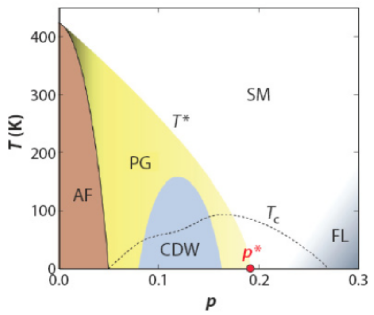
Figure 8: Typical phase diagram of hole – doped cuprates. Superconducting state is observed in the region of temperatures below $T_{c}$, shown by dashed line. Antiferromagnetic region AF is shown in brown. Pseudogap phase PG exists at temperatures below $T^{\star}$ (yellow) and ends at $T=0$ in the critical point $p^{\star}$ (red dot). Inside the pseudogap phase exists the phase with charge density wave CDW (blue). The region of strange metal SM (white) continuously transforms into the Fermi – liquid region FL at higher dopings. Tail

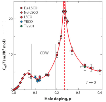
Figure 9: Electronic specific heat coefficient $\gamma=C_{el}/T$ in normal state ($T=$5K) in the vicinity of the quantum critical point (superconductivity is suppressed by external magnetic field) as function of doping $p$ for La_1.8-xEu_0.2Sr_xCuO₄ (Eu-LSCO, red squares), La_1.6-xNd_0.4Sr_xCuO₄ (Nd-LSCO, red circles), La_2-xSr_xCuO₄ (LSCO, red diamonds), YBa₂Cu₃O_y (YBCO, blue circles) and Tl₂Ba₂CuO_6-δ (Tl2201, green circles) Tail

This diagram is well – known for a long time, but what is important for us now is the possible existence here of a quantum critical point Sachd ; Stish at carriers (holes) concentration $p=p^{\star}$, where the pseudogap region ends SadPG ; SadLPI ; GDMFT . Experimental evidence in favor of the existence of such a critical point are rather numerous Tail . As an example in Fig. 9 we just show one of the most striking – the sharp singularity of the electronic specific heat coefficient $\gamma=C_{el}/T$ at $p=p^{\star}$ in the normal state of cuprates, obtained in a strong magnetic field suppressing superconductivity Tail .

The nature of the pseudogap state in cuprtaes is not completely clarified by now. In particular, it is not clear, whether PG region on the phase diagram of Fig. 8 is some new phase and the line $T^{\star}$ defines the critical temperature of a true phase transition, or it is the region of some crossover to antiferromagnetic phase AF, with well developed fluctuations of AF short – range order SadPG ; SadLPI ; GDMFT . antiferromagnetic scenario of pseudogap formation also has a serious experimental support Tail , though some authors believe, that the transition to pseudogap phase is some true phase transition with some still unknown order parameter. A number of specific models (see e.g. Varma ) of such phase transition were proposed, allowing to consider $p=p^{\star}$ as a true quantum critical point. However, it is still unclear, whether we can speak of the quantum critical point in crossover scenario. In any case, the $T$ – linear behavior of resistivity in cuprates is observed close to optimal doping, which nearly coincides with $p=p^{\star}$. To the left of this concentration resistivity demonstrates some dielectric (localization) effects (the strong negative temperature coefficient of resistivity) SadLoc , while to the right we have a crossover to more or less usual Fermi – liquid – like behavior with quadratic growth of resistivity with temperature.

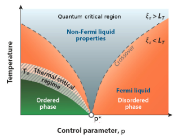
Figure 10: Phase diagram in the vicinity of the quantum critical point. Non – Fermi – liquid behavior of relaxation rate and resistivity can be observed in the quantum critical region, where $\xi_{\tau}>L_{T}=\frac{\hbar}{k_{B}T}$, which corresponds to $\hbar\Omega_{0}<k_{B}T$

.

the closeness of the system to the quantum critical point can, in principle, explain the $T$ – linear growth of resistivity even within the elementary model considered above, To observe such growth at low temperatures, it is sufficient to satisfy the inequality $\Omega_{0}\ll T$, where $\Omega_{0}$ is a characteristic frequency of fluctuations, scattering the electrons. In the vicinity of the quantum critical point (of any nature) we can expect the typical “softening” of the appropriate fluctuation mode according to the relation Sachd ; Stish :

$$\Omega_{0}\sim|p-p^{\star}|^{z\nu}$$ (62)

where $p$ is e.g. the concentration of carriers (holes of electrons). Here $\nu$ and $z$ are the standard critical exponents of the theory of quantum phase transitions, determining the critical behavior of characteristic lengths:

$$\xi\sim|p-p^{\star}|^{-\nu},\ \xi_{\tau}\sim|p-p^{\star}|^{-z\nu}$$ (63)

Here $\tau$ denotes the imaginary (Matsubara) time and above we just put $\Omega_{0}\sim\xi_{\tau}^{-1}$.

As shown in Fig. 10 the quantum critical region is defined by inequality Sachd ; Stish :

$$\xi_{\tau}>\frac{1}{T}\quad\mbox{or}\quad\Omega_{0}<T$$ (64)

which may guarantee the $T$ – linear behavior of resistivity in this region in cuprates or similar systems. However, the nature of quantum fluctuations of importance here, as well as the mechanism of their interaction with electrons remain an open question.

V General relations for the Green’s function and conductivity

V.0.1 Green’s function fir the system of interacting particles

Let us remind some general expressions for an arbitrary system of interacting electrons. We have the following general expression for Matsubara Green’s function AGD :

$$G(i\varepsilon_{n},{\bf p})=\frac{1}{i\varepsilon_{n}-\xi_{\bf p}-\Sigma(i\varepsilon_{n},{\bf p})}$$ (65)

Having in mind the electron – phonon coupling and its analogs (quantum fluctuations of a general nature), dropping the momentum dependence of self – energy, we can write down the following expression in the standard notations of Eliashberg – McMillan theory:

$$\Sigma(i\varepsilon_{n})=[1-z(\varepsilon_{n})]i\varepsilon_{n}+\chi(\varepsilon_{n})$$ (66)

Then:

$$G(i\varepsilon_{n},{\bf p})=\frac{1}{z(\varepsilon_{n})i\varepsilon_{n}-\xi_{\bf p}-\chi(\varepsilon_{n})}=$$

$$=\frac{Z(\varepsilon_{n})}{i\varepsilon_{n}-Z(\varepsilon_{n})\xi_{\bf p}-Z(\varepsilon_{n})\chi(\varepsilon_{n})}$$ (67)

where we have defined:

$$Z(\varepsilon_{n})=z^{-1}(\varepsilon_{n})$$ (68)

Let us define also:

$$\varepsilon({\bf p},\varepsilon_{n})=Z(\varepsilon_{n})\xi_{\bf p}+Re\chi(\varepsilon_{n})$$ (69)

$$\Gamma_{i}(T)sign\varepsilon_{n}=-2Z(\varepsilon_{n})Im\chi(\varepsilon_{n})$$ (70)

Then the Green’s function can be written in the following general enough form:

$$G(i\varepsilon_{n},{\bf p})=\frac{Z(\varepsilon_{n})}{i\varepsilon_{n}-\varepsilon({\bf p},\varepsilon_{n})+\frac{i}{2}\Gamma(T)sign\varepsilon_{n}}$$ (71)

If there is no dependence on $\varepsilon_{n}$ in (69) we can write the Green’ function in the usual form:

$$G(i\varepsilon_{n},{\bf p})=\frac{Z}{i\varepsilon_{n}-\varepsilon({\bf p})+\frac{i}{2}\Gamma(T)sign\varepsilon_{n}}$$ (72)

which is sufficient for our aims.

These expressions more or less correspond to the usual picture of electron – phonon interaction, when $\lambda\ll 1$, though we can try to “drag” them to the region of $\lambda>1$, using the Migdal theorem Diagram , which allows to neglect vertex corrections. In particular, in this approach the renormalization factor is: Diagram

$$Z=\frac{1}{1+\lambda}$$ (73)

and does not depend explicitly on $\varepsilon_{n}$. Eq. (73) is valid within an energy layer of the order of double Debye frequency around the Fermi level (in case of interaction with phonons) or the double average frequency of fluctuations $<\Omega>$. Outside this layer it is obvious that $Z=1$ – fluctuations are practically irrelevant for electrons of high – enough energy.

V.0.2 General expressions for conductivity

Diagonal element of conductivity tensor at ${\bf q}=0$ can be written as: Diagram ; Fuku

$$\sigma_{xx}(\omega)=\frac{1}{i\omega}\left\{\Phi_{xx}(\omega+i\delta)-\Phi_{xx}(0+i\delta)\right\}$$ (74)

where:

$$\Phi_{xx}(i\omega_{m})=-2eT\sum_{n}\sum_{\bf p}\frac{p_{x}}{m}J_{x}({\bf p,p,}\varepsilon_{n},\varepsilon_{n}+\omega_{m})\times$$

$$\times G(\varepsilon_{n}{\bf p})G(\varepsilon_{n}+\omega_{m}{\bf p})$$ (75)

which corresponds to the usual loop diagram shown in Fig. 11, where the “current” vertex can be written as:

$$J_{\mu}({\bf p,p},\varepsilon_{n},\varepsilon_{n}+\omega_{m})\equiv\frac{e}{m}p_{\mu}\Xi({\bf p},\varepsilon_{n},\varepsilon_{n}+\omega_{m})$$ (76)

and the “bare” current vertex is $\frac{e}{m}p_{\mu}$.

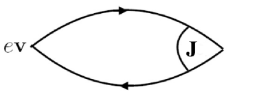
Figure 11: Loop diagram determining conductivity.

Then rewriting Eq. (75) as:

$$\Phi_{xx}(i\omega_{m})=-2e^{2}T\sum_{n}\sum_{\bf p}\frac{p_{x}^{2}}{m^{2}}\Xi({\bf p},\varepsilon_{n},\varepsilon_{n}+\omega_{m})\times$$

$$\times G(\varepsilon_{n}{\bf p})G(\varepsilon_{n}+\omega_{m}{\bf p})$$ (77)

and performing the standard summation over $n$ and analytic continuation $i\omega_{m}\to\omega+i\delta$ Fuku , we obtain the static conductivity at $(\omega\to 0)$:

$$\sigma_{xx}=\frac{e^{2}}{2\pi}\sum_{\bf p}\frac{p_{x}^{2}}{m^{2}}\Xi({\bf p})G^{R}({\bf p},0)G^{A}({\bf p},0)$$ (78)

where we have introduced the static limit $\Xi({\bf p})=\Xi({\bf p},0-i\delta,0+i\delta)$.

Obviously, the main difficulty here is related to the explicit calculation of the vertex part for the system of interacting particles. The simplest estimate can be obtained using in Eq. (75) the obvious Ward identity Fuku , which is valid for $\omega_{m}=0$:

$$J_{\mu}({\bf p,p},\varepsilon_{n},\varepsilon_{n})=-e\frac{\partial}{\partial p_{\mu}}G^{-1}(\varepsilon_{n},{\bf p})=$$

$$=-e\left[-v_{\bf p}^{\mu}-\frac{\partial\Sigma(\varepsilon_{n},{\bf p})}{\partial p_{\mu}}\right]$$ (79)

where velocity $v_{\bf p}^{\mu}=\frac{\partial\xi_{\bf p}}{\partial p_{\mu}}$. If we assume here that the self – energy is momentum independent i.e. $\Sigma(\varepsilon_{n},{\bf p})=\Sigma(\varepsilon)$, as it usually takes place for electron – phonon interaction, the vertex (79) is reduced to the “bare” one:

$$J_{\mu}({\bf p,p},\varepsilon_{n},\varepsilon_{n})=ev_{\bf p}^{\mu}=\frac{e}{m}p_{\mu}$$ (80)

which corresponds to $\Xi({\bf p},\varepsilon_{n},\varepsilon_{n})=1$. Using (79) in (75) we get:

$$\Phi_{xx}(i\omega_{m})=-2e^{2}T\sum_{n}\sum_{\bf p}\frac{p_{x}}{m}\left[\frac{\partial}{\partial p_{\mu}}G^{-1}(\varepsilon_{n},{\bf p})\right]\times$$

$$\times G(\varepsilon_{n}{\bf p})G(\varepsilon_{n}+\omega_{m}{\bf p})=$$

$$=-2e^{2}T\sum_{n}\sum_{\bf p}\frac{p_{x}^{2}}{m^{2}}G(\varepsilon_{n}{\bf p})G(\varepsilon_{n}+\omega_{m}{\bf p})$$ (81)

and then, making all transformations as in going from (75) to (78) we obtain the following expression approximate relation for static conductivity:

$$\sigma_{xx}=\frac{e^{2}}{2\pi}\sum_{\bf p}\frac{p_{x}^{2}}{m^{2}}G^{R}({\bf p},0)G^{A}({\bf p},0)$$ (82)

which simply corresponds to the choice of $\Xi({\bf p})=1$ in (78). In contrast to (78) this is certainly a kind of approximation. It is used e.g. in Ref. Varma . What is lost here will become clear below.

Further calculations will be done for the general case of (78). Keeping in mind the typical metal, where all the physics of conductivity is determined in the vicinity of the Fermi surface (and scattering is rather weak), we can use the usual integration over the energy spectrum linearized close to the Fermi level and write (78) as ($Re\Sigma(0)$ can be included in the renormalization of the chemical potential):

$$\sigma_{xx}=\frac{e^{2}}{2\pi}N(0)\int_{-\infty}^{\infty}d\xi_{p}\frac{1}{3}\frac{p_{F}^{2}}{m^{2}}\Xi(p_{F})G^{R}({\bf p},0)G^{A}({\bf p},0)=$$

$$=\frac{e^{2}}{2\pi}\frac{1}{3}v_{F}^{2}\Xi(p_{F})N(0)\int_{-\infty}^{\infty}d\xi_{p}\frac{1}{\xi_{p}^{2}+Im^{2}\Sigma(0)}=$$

$$=e^{2}\frac{1}{3}v_{F}^{2}N(0)\frac{\Xi(p_{F})}{2Im\Sigma(0)}\equiv\frac{ne^{2}}{m}\tau_{tr}$$ (83)

From this expression it is clear, by the way, that approximation $\Xi(p_{F})=1$ corresponds to neglecting the difference between $\tau$ and $\tau_{tr}$, which we used everywhere above. For the case of scattering by point – like impurities or Einstein phonons this is simply always valid – from (83) we immediately get (48). Precisely the same expression for conductivity is used e.g. in Ref. Varma . Now it is clear that the mass renormalization, appearing e.g. in the expression for electronic specific heat does not enter the expression for $\sigma_{xx}$, where everything is determined by the “bare” (band) mass. This result is well – known actually for a long time Naka ; PrKad ; Hein ; Grim .

Contribution from the possible momentum dependence of $\Sigma(\varepsilon,{\bf p})$ into static conductivity also can be obtained in rather simple way Fuku . Let us write:

$$G^{R}(\varepsilon,{\bf p})=[Z^{-1}\varepsilon-b^{-1}\xi_{p}+Im\Sigma(\varepsilon,p_{F})]^{-1}$$ (84)

where as usual we introduced:

$$Z^{-1}=1-\frac{\partial}{\partial\varepsilon}Re\Sigma(\varepsilon,p_{F})|_{\varepsilon=0}$$ (85)

$$b^{-1}=1+\frac{\partial}{\partial\xi_{p}}Re\Sigma(0,{\bf p})|_{|\bf p|=p_{F}}$$ (86)

Then, using Eq. (84), we obtain density of stets renormalization on the Fermi level and get:

$$\tilde{N}(0)=-\frac{1}{\pi}\sum_{\bf p}ImG^{R}(0,{\bf p})=\frac{1}{\pi}\int_{-\infty}^{\infty}d\xi_{p}\frac{1}{b^{-2}\xi_{p}+Im\Sigma(0,{\bf p})}=bN(0)$$ (87)

Now we may repeat all calculations for conductivity done above using (84), and obtain the final result for static conductivity as: Fuku :

$$\sigma_{xx}=\frac{ne^{2}}{m}\frac{\Xi(p_{F})}{2Im\Sigma(0)}b=\frac{ne^{2}}{m}\tau_{tr}\frac{\tilde{N}(0)}{N(0)}$$ (88)

V.0.3 Self – consistent calculation

Let us return to the simplest model of electron – phonon interaction and make the self – consistent calculation, when electron line on diagram of Fig. 7 is “dressed”, i.e. takes into account all orders of non – intersecting interaction lines. Again we assume the validity of Migdal’s theorem Diagram . Acting in the spirit of Eqs. (66) – (72), we can write the expression for the Green’s function as (simplified variant of Eq. (71)):

$$G(\varepsilon_{n},{\bf p})=\frac{Z}{i\varepsilon_{n}-Z\xi_{\bf p}+\frac{i}{2}Z\Gamma(T)sign\varepsilon_{n}}$$ (89)

which corresponds to a choice of $Z(\varepsilon_{n})=Z$ $Re\chi(\varepsilon_{n})=0$, $Im\chi(\varepsilon_{n})=-\Gamma(T)$ in Eq. (67). Renormalization factor $Z<1$ is assumed to be a constant for simplicity. Then it may seem, that taking $\Gamma_{i}(T)=2\pi\lambda T$ we may introduce the renormalized damping as:

$$\tilde{\Gamma}(T)=Z\Gamma(T)=2\pi\lambda ZT=2\pi\frac{\lambda}{1+\lambda}T$$ (90)

where we have accounted for the known result due electron – phonon interactions in low – temperature limit Diagram :

$$Z=\frac{1}{1+\lambda}$$ (91)

Accordingly, for $\lambda\ll 1$ we have (46), and for $\lambda\gg 1$ we get:

$$\tilde{\Gamma}(T)=2\pi T$$ (92)

i.e. the universal “Planckian” behavior of relaxation rate (21) with $\alpha=2\pi$ independent of coupling constant of electrons with fluctuations (phonons). In general case, for arbitrary values of $\lambda$ we have $\alpha<2\pi$, so that the upper limit for $\alpha$ appears in a natural way and is defined by (92).

However, substituting (89) into (44), which is obtained in high – temperature limit, in the model with Einstein spectrum of fluctuations (phonons) we immediately obtain:

$$\Sigma(\varepsilon_{n},{\bf p})=\Sigma(\varepsilon_{n})=-i\pi\frac{2g_{0}^{2}}{\Omega_{0}}N(0)Tsign\varepsilon_{n}=-\frac{i}{2}\Gamma(T)sign\varepsilon_{n}$$ (93)

so that the renormaliztion factor $Z$ in damping is canceled out and we just reproduce the usual result derived above without any renormalizations. This is not surprising at all — it is clear from the very beginning that $Z\approx 1$ for temperatures (energies) much higher than characteristic phonon frequencies (or any other fluctuation quanta scattering the electrons). Similar results are valid not only in Einstein model, but also in the general case, described by Eliashberg – McMillan approximation (51), (60) Sad20 .

It may also seem, that limitations discussed above may be obtained from completely different considerations. Let us write down the general enough expression for Matsubara Green’s function in high – temperature limit as:

$$G(i\varepsilon_{n},{\bf p})=\frac{1}{i\varepsilon_{n}-\varepsilon_{\bf p}+\frac{i}{2}\Gamma(T)sign\varepsilon_{n}}$$ (94)

After substitution here the limiting value of $\Gamma(T)$ from (21) we obtain:

$$G(i\varepsilon_{n},{\bf p})=\frac{1}{i\varepsilon_{n}-\varepsilon_{\bf p}+\frac{i}{2}\alpha Tsign\varepsilon_{n}}$$ (95)

Then we immediately see that the constant $\alpha$, seemingly, can not achieve the value of $\alpha=2\pi$, as Matsubara frequencies in (95) become in this case even, i.e. the system of fermions “turns” into bosons, which is just impossible because of the general spin – statistics theorem — no interaction (leading e.g. to temperature – dependent relaxation) can not change the statistics of particles. Then, apparently, we have to introduce the same limitation again:

$$\Gamma(T)=\frac{1}{\tau(T)}<2\pi T$$ (96)

that in particular means that in our model according to Eq. (61) we always have an inequality $\lambda<1$. Such limitation on coupling constant agrees with recent results of quantum Monte – Carlo calculations of electron – phonon interactions Scal , but contradicts many years of experience in studies of superconductivity within Eliashberg – McMillan theory Savr ; Alle . Discussion of these contradictions and possible solutions can be found in the recent paper ChuKiv .

In fact, the arguments given above are incorrect and the value of $\alpha$ can can take any values including integers, with no paradoxes like the change of statistics. These values are not special and the system may continuously pass through them with the growth of $\alpha$ (i.e. the coupling strength). This can be easily understood making e.g. explicit calculations of distribution function (cf. Appendix).

It should be noted of course, that the $T$ – linear behavior of damping in the Green’s function in all cases breaks the standard criteria for Fermi – liquid behavior PinNoz , so that quasiparticles in the system are badly defined. This is also seen from the explicit form distribution function, which is rather far from the usual Fermi step – like function.

V.0.4 Planckian relaxation delusion

In Refs. Bruin ; Legros experimental data on resistivity were represented by Drude expression (13), where the effective mass $m^{\star}$ was determined from measurements of specific heat or de Haas – van Alfen effect, which in the model with electron – phonon or in a more general model of scattering by quantum fluctuations of an arbitrary nature, is obtained from the band structure effective mass by a simple substitution $m\to m^{\star}=m(1+\lambda)$, which takes into account mass renormalization by interactions (at low temperatures!). Inconsistency of this approach was already stressed in Ref. Varma . Leta us show, that precisely this representation of experimental data leads to to the delusion of universal Planckian relaxation in metals. In fact Eq. (48) for the high – temperature limit of resistivity can be identically rewritten as:

$$\rho(T)=\frac{m(1+\lambda)}{ne^{2}}\frac{\Gamma(T)}{1+\lambda}=\frac{m^{\star}}{ne^{2}}\tilde{\Gamma}(T)$$ (97)

where

$$\tilde{\Gamma}(T)=2\pi\frac{\lambda}{1+\lambda}T$$ (98)

which always leads to:

$$\tilde{\Gamma}(T)<2\pi T$$ (99)

just imitating the universal “Planckian” behavior of relaxation rate (21) with $\alpha=2\pi$ as an upper limit independent of coupling constant of electron with fluctuations (phonons). The substitution of $m\to m^{\star}=m(1+\lambda)$ in (97) by itself is correct, despite being used in an expression in high – temperature limit. Also correct is the treatment of experimental data in Refs. Bruin ; Legros , where they used the effective mass $m^{\star}$, obtained from low – temperature measurements. However, this approach clouds the crux of the matter, creating the delusion of universal Planckian behavior.

It is easy to estimate that the experimentally observed Bruin ; Legros values of $\alpha\sim 1$ correspond to rather typical $\lambda\sim 0.2$, while $\alpha\sim 2.8$ for lead Bruin corresponds to $\lambda\sim 0.53$. Calculations within Eliashberg – McMillan theory for Pb give $\lambda\sim 1.5$ Savr . For Nb in Ref. Bruin was found that $\alpha\sim 2.3$, which according to expressions given above corresponds to $\lambda\sim 0.43$, while the calculations Savr give $\lambda\sim 1.26$. Suppression by a factor of $\sim 3$ of our values of $\lambda$ may be possibly related to the fact, that in expressions for resistivity we must use $\lambda_{tr}<\lambda$. However, the calculated values of $\lambda_{tr}$ Savr equal 1.19 for Pb and 1.17 for Nb, which does not improve much the agreement with experiments.

Much more important may be the account of mass renormalization due to electron – electron interactions, which also contribute to electronic specific heat. which in practice is difficult to separate from phonon contribution. Accordingly, Eq. (98) should be rewritten as:

$$\tilde{\Gamma}(T)=2\pi\frac{\lambda}{1+\lambda+\lambda_{ee}}T$$ (100)

where we have introduced $\lambda_{ee}$ – the dimensionless parameter, determining mass renormalization due to electron – electron interaction. In Landau – Silin Fermi – liquid theory $\lambda_{ee}=\frac{F^{s}_{1}}{3}$, where $F^{s}_{1}$ is the appropriate coefficient in the expansion of Landau function PinNoz . For typical metals $\lambda_{ee}\sim 1$. Then:

$$\alpha=\frac{2\pi\lambda}{1+\lambda+\lambda_{ee}}$$ (101)

so that taking as typical $\lambda\sim 0.4$ and $\lambda_{ee}\sim 1$ we immediately obtain $\alpha\sim 1.04$, while for $\lambda\sim 0.5$ we have $\alpha\sim 1.25$, in goof agreement with majority of the data of Refs. Bruin ; Legros . For Pb, taking $\lambda=1.68$ Savr and $\lambda_{ee}=1$ we get $\alpha\sim 2.86$ in reasonable agreement with “experimental” value of $\alpha=2.8$ Bruin . Similarly, for Nb we have $\lambda=1.26$ Savr , so that again using $\lambda_{ee}\sim 1$ we obtain $\alpha\sim 2.42$, in good agreement with “experimental” value of $\alpha=2.3$ Bruin . The interval of the values of $\alpha=0.7-2.8$ Bruin ; Legros for $\lambda_{ee}=1$ corresponds to the interval of $\lambda=0.25-1.5$, that seems quite reasonable.

More detailed results of such estimates (assuming $\lambda_{ee}=1$) are given in the Table:

Metal	$\lambda$	$\frac{2\pi\lambda}{1+\lambda}$	$\frac{2\pi}{1+\lambda+\lambda_{ee}}$	$\alpha_{exp}$
Pb	1.68	3.93	2.86	2.8
Nb	1.26	3.50	2.42	2.3
Cu	0.14	0.77	0.41	1.0
Al	0.44	1.91	1.13	1.1
Pd	0.35	1.63	0.93	1.1

Now we can see, that for all metals under consideration here, with the exception of Cu, experimental data on coefficient $\alpha$ are described rather satisfactory and full agreement can be achieved by minor variations of $\lambda_{ee}$ around the value of $\lambda_{ee}=1$. This is not so only for Cu, where the agreement can be reached by introduction of $\lambda_{ee}<0$. The negative values of $\lambda_{ee}$ are possible, taking into account that the general limitation here PinNoz is $F^{s}_{1}>-3$, i.e. $\lambda_{ee}>-1$.

Thus we came to the main conclusion – the “experimentally” observed universal Planckian relaxation in metals, independent of the value of the coupling constant, is nothing more than delusion, related to the procedure of representation of experimental data in Refs. Bruin ; Legros (determination of the effective mass in the expression for resistivity from low – temperature measurements). Similarly, the same applies to the results of a recent paper Cao , where this procedure was used to represent experimental data on bilayer graphene near the “magic” angle of (mis)orientation of the layers.

V.0.5 Once again on uncertainty principle

Where is the problem with the estimates of relaxation time based on energy – time uncertainty relation? This is rather simple – in Eq. (20) $\Delta E$ should be taken not as $k_{B}T$, but as a real “level width” (spectrum damping) in the system of many interacting (!) particles:

$$\Gamma(T)=2\pi\lambda T$$ (102)

Then we immediately have:

$$\frac{\hbar}{\tau}\leq 2\pi\lambda T$$ (103)

so that the use of uncertainty relation becomes a kind of tautology. Then the “upper limit” of high – temperature relaxation rate is not universal and naturally proportional to the coupling constant.

At the same time, the result of Eq. (99) obtained above, formally defines some universal upper limit for relaxation rate of quasiparticles, so that the estimates based on uncertainty relation probably can be applied here.

VI Conclusions

As we stressed above, our aims did not included the explanation of $T$ – linear growth of resistivity, starting from the lowest temperatures, which is observed in copper oxides high – temperature superconductors and some similar systems. In the models of scattering by quantum fluctuations of an arbitrary nature (e.g. phonons), such behavior appears at temperatures of the order or higher than the characteristic frequency of these fluctuations, i.e. in the classical limit. At present it is unclear whether such low – frequency fluctuations exist in the vicinity of the quantum critical point on the phase diagram of cuprates, which could have explained their anomalous behavior. But this a simplest calculable model which clearly shows, that the universal Planckian behavior of relaxation rate is just absent, as well is just absent is the universal upper limit for this relaxation rate. Dependence on the interaction parameters in relaxation rate does not disappear and it can, in principle, easily overcome the limit of $\alpha\sim 1$.

In the literature, quite a number of microscopic models were proposed, explaining the $T$ – linear growth of resistivity (inelastic scattering rate) in metals. We have already mentioned Refs. Khod ; Khodel ; Vol , where this behavior appeared in the model of “fermion” condensation and was related, in particular, to formation of “flat” bands near the Fermi level and appearance of low – frequency zero – sound excitations, so that scattering by these excitations leads to $T$ – linear growth of scattering rate. In Ref. Sachdev an interesting model was proposed with random interactions of electrons, where the “flat” band also forms and for the wide interval of parameters the $T$ – linear growth of resistivity is realized. It is unclear however, which relation if any at all the model of interactions assumed in Ref. Sachdev has to real metals. Note also, that in all these approaches the universal “Planckian” dependence on temperature does not appear, and dependence on the coupling strength (though probably a weak one) is conserved. Similar situation is realized in a popular phenomenological model of marginal Fermi – liquid Varma , which successfully explains many properties of cuprates.

An interesting model was proposed recently in Ref. Mous to explain the anomalous temperature dependence of resistivity in Sr₃Ru₂O₃ by electron – electron scattering processes, taking into account rather complicated real electronic spectrum of this compound, leading to many – sheets of the Fermi surface, with some special “hot” pockets, where electron are non – degenerate (classical limit). It is the scattering of electrons from “cold” (degenerate) parts of the Fermi surface, with transition of one of these electron to the “hot” pocket, which leads to the linear growth of resistivity with temperature. The analogy with the model with scattering by non – degenerate fluctuations (classical limit) considered above is pretty obvious. Of course, the dependence on the value of the appropriate coupling constant does not disappear, and the “universal” Palnckian behavior appears only for the renormalized (in a sense discussed above) scattering rate of the quasiparticles.

The special place is occupied by Refs. Zan ; Hart ; Herz ; Hartn , based on the analogies taken from black hole physics, cosmology and superstring theory, which pretend to explain the universal “Planckian” behavior of the relaxation rate. Being very interesting from theoretical point of view these papers, in our opinion, have a weak relation to solid state physics.

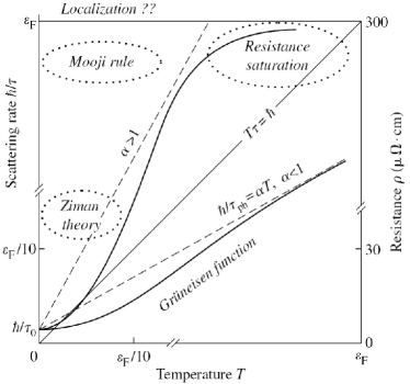
Figure 12: Temperature – disorder plane ($T$,$\hbar/\tau$), where regions of applicability of different models of electrical resistivity are shown. Also shown are temperature dependencies of resistivity. “Planckian” relaxation rate determines the diagonal on this plane.Gant

In this paper we have limited ourselves to elementary analysis based on the standard approaches of the solid state theory and shown, that the observed universal “Planckian” behavior of electron relaxation rate in many metals Bruin ; Legros has rather simple explanation, related not to some special deep physics, but simply to the method of representation of experimental data used in these papers. The use in Drude expression for conductivity (resistivity) of the effective mass, determined from low – temperature measurements, which includes the renormalization due to many – particle effects (interactions), inevitably leads to appropriate renormalization of relaxation rate (time), which is replaced by an effective rate $\tilde{\Gamma}$ (98) of relaxation for quasiparticles, which is relatively weakly dependent on the coupling strength and, in principle, produces the universal “Planckian” behavior, as an upper limit for this relaxation rate. However, this behavior is a pure delusion and does not reflect any kind of special physics. In microscopic theory it is the unrenormalized (by interactions) band mass, which enters the Drude expression for conductivity, and relaxation rate is naturally proportional to the strength of interaction, as was well – known since the early days of quantum solid state theory.

The size of an effective relaxation rate $\hbar/\tau=k_{B}T$ (i.e. in fact the “Planckian” rate discussed above) in a standard theory, as is also well – known, defines some characteristic scale, which separates regions of different behavior of resistivity of metals, as it is shown in Fig. 12, taken from the textbook Gant . There we also show characteristic temperature dependencies of resistivity of metals. “Planckian” scattering rate determines the diagonal on this figure, but does not define any new quantum limit . In principle, all this is known for a long time and does not require any “exotic” approaches for its explanation.

The author is grateful to E.Z. Kuchinskii and D.I. Khomskii for useful discussions. This work was partially supported by RFBR grant No. 20-02-00011.

Appendix A Momentum distribution in case of Planckian relaxation

Consider the momentum distribution corresponding to Green’s function (95):

$$N({\bf p})=T\sum_{n}G(i\varepsilon_{n},{\bf p})$$ (104)

Performing the standard summation over fermion Matsubara frequencies Diagram , we obtain:

$$N({\bf p})=-\frac{1}{2\pi i}\int_{c}d\varepsilon f(\varepsilon)G(\varepsilon,{\bf p})=$$

$$-\frac{1}{2\pi i}\int_{-\infty}^{\infty}d\varepsilon f(\varepsilon)(G^{R}(\varepsilon,{\bf p})-G^{A}(\varepsilon,{\bf p}))=\int_{-\infty}^{\infty}d\varepsilon f(\varepsilon)A(\varepsilon,{\bf p})$$ (105)

where $f(\varepsilon)=\frac{1}{e^{\varepsilon/T}+1}$ is Fermi distribution, and spectral density $A(\varepsilon,{\bf p})=-\frac{1}{\pi}ImG^{R}(\varepsilon,{\bf p})$ for Green’s fuction (95) is given by Lorentzian:

$$A(\varepsilon,{\bf p})=\frac{1}{\pi}\frac{\frac{\alpha}{2}T}{(\varepsilon-\varepsilon_{\bf p})^{2}+(\frac{\alpha}{2}T)^{2}}$$ (106)

In Fig. 13 we show distribution functions $N({\bf p})$, obtained numerically directly from (105) with spectral density (106) for different values of $\alpha$. However, for special $\alpha=2\pi n$ $n=0,1,\cdots$, distribution functions can be obtained analytically. For $\alpha=0$ we obviously get the usual Fermi distribution $N({\bf p})=f(\varepsilon_{\bf p})$. For $\alpha=2\pi$ we obtain:

$$G(i\varepsilon_{n},{\bf p})=\frac{1}{i\varepsilon_{n}-\varepsilon_{\bf p}+i\pi Tsign\varepsilon_{n}}=\frac{1}{i2\pi Tm-\varepsilon_{\bf p}}$$ (107)

where $m$ is an integer, but $sign\varepsilon_{n}$ excludes the value of $m=0$. Then the distribution function of particles is:

$$N({\bf p})=T\sum_{n}G(i\varepsilon_{n},{\bf p})=T\sum_{m\neq 0}\frac{1}{i2\pi Tm-\varepsilon_{\bf p}}=$$

$$=T\sum_{m}\frac{1}{i2\pi Tm-\varepsilon_{\bf p}}+\frac{T}{\varepsilon_{\bf p}}$$ (108)

Note that the sign before summation over seemingly even Matsubara frequencies remained the same (fermion – like), which is related to initial summing over odd frequencies. The second term in the last expression in (108) compensated the contribution of $m=0$, which appeared in sum over $m$ in the first term. Making the standard summation over even frequencies $\varepsilon_{m}=2\pi Tm$ we get:

$$T\sum_{m}\frac{1}{i\varepsilon_{m}-\varepsilon_{\bf p}}=\frac{1}{2\pi i}\int_{c}d\varepsilon\frac{1}{\varepsilon-\varepsilon_{\bf p}\pm i\delta}n(\varepsilon)=$$

$$=\frac{1}{\pi}\int_{-\infty}^{\infty}d\varepsilon Im\frac{1}{\varepsilon-\varepsilon_{\bf p}+i\delta}n(\varepsilon)=-\int_{-\infty}^{\infty}d\varepsilon\delta(\varepsilon-\varepsilon_{\bf p})n(\varepsilon)=$$

$$=-n(\varepsilon_{\bf p})$$ (109)

where $n(\varepsilon)=\frac{1}{e^{\varepsilon/T}-1}$ is Bose distribution.

Thus, for $\alpha=2\pi$:

$$N({\bf p})=\frac{T}{\varepsilon_{\bf p}}-n(\varepsilon_{\bf p})$$ (110)

Note once again, that the minus sign before Bose distribution in (110) is related to initial summation over fermion frequencies.

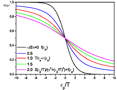
Figure 13: Distribution function for Planckian relaxation with different $\alpha$.

For $\alpha=4\pi$ again we have summation over odd frequencies, but with two closest to zero fermion Matsubara frequencies excluded:

$$N({\bf p})=T\sum_{n}\frac{1}{i\varepsilon_{n}-\varepsilon_{\bf p}+i2\pi Tsign\varepsilon_{n}}=$$

$$=T\sum_{n\neq 0,-1}\frac{1}{i2\pi T(n+\frac{1}{2})-\varepsilon_{\bf p}}=$$

$$=T\sum_{n}\frac{1}{i\varepsilon_{n}-\varepsilon_{\bf p}}-T\left(\frac{1}{i\pi T-\varepsilon_{\bf p}}+\frac{1}{-i\pi T-\varepsilon_{\bf p}}\right)=$$

$$=f(\varepsilon_{\bf p})+\frac{2T\varepsilon_{\bf p}}{\varepsilon_{\bf p}^{2}+(\pi T)^{2}}$$ (111)

In Fig. 13 for $\alpha=2\pi$ and $\alpha=4\pi$ we show both distributions obtained numerically from (105) with spectral density (106) and obtained directly from (110) and (111) (obviously these are identical).

In general, it can be seen that distribution fictions in our model are rather different from the usual step – function of Fermi – liquid theory.

Note added in proofs: After this work was accepted for publication we have learned on the paper by E.H. Hwang, S. Das Sarma. Phys. Rev. B99, 085105 (2019), where the authors came to the same conclusions in the context of electron – phonon interaction.

References

- (1) B. Batlogg. Physics Today 44, 44 (1991)
- (2) I. Iye in “Physical Properties of High Temperature Supeconductors”. Ed. by D.M. Ginsberg, World Scientific, Singapore 1991
- (3) J.A.N. Bruin, H. Sakai, R.S. Perry, A.P. MacKenzie. Science 339, 804 (2013)
- (4) A. Legros, S. Benhabib, W. Tabis, F. Laliberte, M. Dion, M. Lizaire, B. Vignole, D. Vignolles, H, Raffy, Z.Z. Li, P. Auban-Senzier, N. Doiron-Leyraud, P. Fournier, D. Colson, L.Taillefer, C. Proust. Nature Physics 15, 142 (2019)
- (5) W. Meissner. Handbuch der Physik, 11, 338 (1935)
- (6) J.M. Ziman. Electrons and Phonons. Clarendon Press, Oxford, 1960
- (7) E.G. Maksimov, Usp. Fiz. Nauk 170, 1033 (2000)
- (8) S. Martin, A,T, Fiory, R.M. Fleming, L.F. Schneemeyer, J.V. Waszczak. Phys. Rev. B41, 846 (1990)
- (9) J. Zaanen. Nature 430, 512 (2004)
- (10) V.R. Shaginyan, K.G. Popov, V.A. Khodel. Phys. Rev. B 88, 115103 (2013)
- (11) V.R. Shaginyan, M.Ya. Amusia, A.Z. Msezane, V.A. Stephanovich, G.S. Japaridze, S.A. Artamonov. JETP Letters 110, 290 (2019)
- (12) A.A. Patel, S. Sachdev. Phys. Rev. Lett. 123, 066601 (2019)
- (13) G.E. Volovik. JETP Letters 110, 352 (2019)
- (14) J. Zaanen. Nature 448, 1000 (2007)
- (15) S.A. Hartnoll. Nature Physics 11, 54 (2015)
- (16) C.P. Herzog, P. Kovtun, S. Sachdev, D.T. Son. Phys. Rev. D 75, 085020 (2007)
- (17) S.A. Hartnoll, P.K. Kovtun, M. Muller, S, Sachdev. Phys, Rev. B 76, 144502 (2007)
- (18) M.V. Sadovskii. Diagrammatics. World Scientific, Singapore, 2019
- (19) A.F. Ioffe, A.R. Regel. Progr. Semiconductors 4, 237 (1960)
- (20) N.F. Mott. Metal – Insulator Transitions. Taylor and Francis, London, 1974
- (21) E. Abrahams, P.W. Anderson, D.C. Licciardello, T.V. Ramakrishnan. Phys. Rev. Lett. 42, 673 (1979)
- (22) M.V. Sadovskii. Usp. Fiz. Nauk 133, 223 (1980) [M.V. Sadovskii, Sov. Phys. – Uspekhi 24, 96 (1981)]
- (23) D. Vollhard, P. Wölfle. In “Electronic Phase Transitions”. Ed. by W. Hanke and Yu. V. Kopaev, North – Holland, Amsterdam, 1990
- (24) P. Markos. Acta Physica Slovaca 56, 561 (2006)
- (25) V.F. Gantmakher. Electrons and Disorder in Solids. Clarendon Press, Oxford, 2005
- (26) J.H. Mooij. Physics Status Solidi (a) 17, 521 (1973)
- (27) M. Gurvitch, A.T. Fiory. Phys. Rev. Lett. 59, 1337 (1987)
- (28) H. Takagi, B. Batlogg, H.L. Kao, J. Kwo, R.J. Cava, J.J. Krajewski, W.F. Peck. Phys. Rev. Lett. 69, 2975 (1992)
- (29) N.E. Hussey, K. Takenaka, H. Takagi. Phil. Mag. 84, 2847 (2004)
- (30) N.R. Poniatowski, T. Sarkar, S. Das Sarma, R.L. Greene. Phys. Rev. B 103, L020501 (2021)
- (31) J. Zaanen (unpublished talks)
- (32) P.B. Allen, B. Mitrović. Solid State Physics (Ed. by F. Seitz, D. Turnbull, D. Ehrenreich), Vol. 37, p. 1, Academic Press, NY, 1982
- (33) P.B. Allen. Phys. Rev. B3, 305 (1971)
- (34) S.Y. Savrasov, D.Y. Savrasov. Phys. Rev. B 54, 16487 (1996)
- (35) I. Esterlis, B. Nosarzewski, E.W. Huang, D. Moritz, T.P. Devereux, D.J. Scalapino, S.A. Kivelson. Phys. Rev. B 97, 140501(R) (2018)
- (36) M.V. Sadovskii. Pis’ma Zh. Eksp. Teor, Fiz. 111, 203 (2020) [M.V. Sadovskii. JETP Letters 111, 188 (2020)]
- (37) A.A. Abrikosov, L.P. Gorkov, I.E. Dzyaloshinskii. Methods of Quantum Field Theory in Statistical Physics. Pergamon Press, Oxford, 1963
- (38) J.M. Ziman. Models of disorder, Cambridge University Press, Cambridge, 1979
- (39) S.F. Edwards. Phil. Mag. 6, 617 (1961); Proc. Roy. Soc. A267, 518 (1962)
- (40) D. Pines. The Many Body Problem, W.A. Benjamin, NY, 1961
- (41) D. Pines. P. Nozieres. The Theory of Quantum Liquids, Vol. 1, W.A. Benjamin, NY, 1966
- (42) C. Proust, L. Taillefer. Annu.Rv.Condens.Matter.Phys. 10, 409 (2019)
- (43) S. Sachdev. Quantum Phase Transitions, Cambridge University Press, Cambridge, 1999
- (44) S.M. Stishov. Usp. Fiz. Nauk 174, 853 (2004)
- (45) M.V. Sadovskii. Usp. Fiz. Nauk 171, 539 (2001) [M.V. Sadovskii, Physics Uspekhi 44, 515 (2001)]
- (46) M.V. Sadovskii. In “Strings, Branes, Lattices, Pseudogap and Dust”. Ed. by M.A. Vasiliev, L.V. Keldysh, A.M. Semikhatov, p. 357, “Scientific World”, Moscow, 2007 [arXiv:cond-mat/0408489]
- (47) E.Z. Kuchinskii, I.A. Nekrasov, M.V. Sadovskii. Usp. Fiz. Nauk 182, 345 (2012) [E.Z. Kuchinskii, I.A. Nekrasov, M.V. Sadovskii. Physics Uspekhi 55, 325 (2012)]
- (48) C.M. Varma. Rev. Mod. Phys.92,031001 (2020)
- (49) M.V. Sadovskii. Physics Reports 282, 225 (1997)
- (50) M.V. Sadovskii. Superconductivity and Localization. World Scientific, Singapore, 2000
- (51) H. Fukuyama, H. Ebisawa, Y. Wada, Prog. Theor. Phys. 42, 494 (1969)
- (52) S. Nakajima, M. Watabe, Prog. Theor. Phys. 29, 341 (1963)
- (53) R.E. Prange, L.P. Kadanoff, Phys. Rev. 134, A566 (1964)
- (54) V. Heine, P. Nozieres, J.W. Wilkins. Phil. Mag. 13, 741 (1966)
- (55) G. Grimvall. Physica Scripta 14, 63 (1978)
- (56) A.V. Chubukov, A. Abanov, I. Esterlis, S.A. Kivelson. Annals of Physics 417, 168190 (2020)
- (57) Y. Cao, D. Chowdhuri, D. Rodan-Legrain, O. Rubies-Bigorda, K. Watanabe, T. Taniguchi, T. Senthil, P. Jarillo-Bigorda. Phys. Rev. Lett. 124, 076801 (2020)
- (58) C.H. Mousatov, E. Berg, S.A. Hartnol. PNAS 117, 2852 (2020)